hypothesis testing
DESCRIPTION
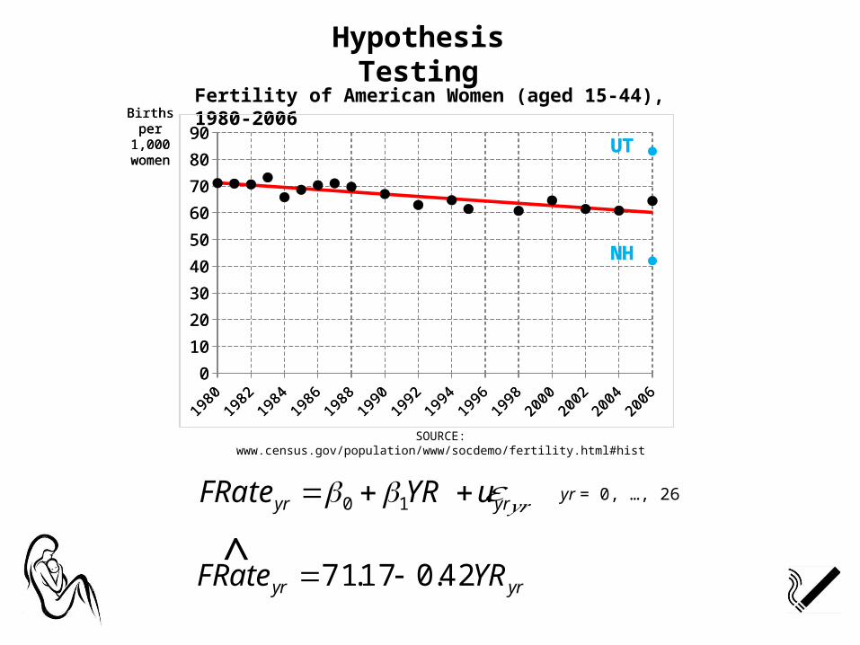
Hypothesis Testing. Fertility of American Women (aged 15-44), 1980-2006. Births per 1,000 women. Births per 1,000 women. UT. UT. NH. NH. SOURCE: www.census.gov/population/www/socdemo/fertility.html#hist. yr = 0, …, 26. ^. Hypothesis Testing of. - PowerPoint PPT PresentationTRANSCRIPT
Hypothesis Testing
1980 1982 1984 1986 1988 1990 1992 1994 1996 1998 2000 2002 2004 20060
10
20
30
40
50
60
70
80
90
SOURCE: www.census.gov/population/www/socdemo/fertility.html#hist
Fertility of American Women (aged 15-44), 1980-2006Births per
1,000 women UT
NH
yryr uYRFRate 10 yr = 0, …, 26𝜀𝑦𝑟
yryr YRFRate 42.017.71 ^
1980 1982 1984 1986 1988 1990 1992 1994 1996 1998 2000 2002 2004 20060
10
20
30
40
50
60
70
80
90Births per
1,000 women UT
NH

tstststs OlderFRateCRate ,,2,10, ln s = 1, …, 47t = 1, …, 13 (1970 to 82)
Hypothesis Testing of 1̂
Suppose you are asked to empirically investigate the charge that obstetricians are guilty of inducing demand by performing unnecessary cesarean sections.
Empirical Model (linear-log)
Panel data𝑙𝑛𝑄𝐶𝑖𝑔𝑖=𝛾0+𝛾1 𝑙𝑛𝑃𝐶𝑖𝑔1+𝜇𝑖
𝛾1=% ∆𝑄𝐶𝑖𝑔% ∆ 𝑃𝐶𝑖𝑔
=¿(%∆𝑄𝐶𝑖𝑔
100 )(% ∆𝑃𝐶𝑖𝑔
100 )𝛽1=
∆𝐶𝑅𝑎𝑡𝑒
(% ∆𝐹𝑅𝑎𝑡𝑒100 ) 𝛽1=
100 ∙ ∆𝐶𝑅𝑎𝑡𝑒%∆𝐹𝑅𝑎𝑡𝑒
∆𝐶𝑅𝑎𝑡𝑒% ∆𝐹𝑅𝑎𝑡𝑒
=𝛽1
100

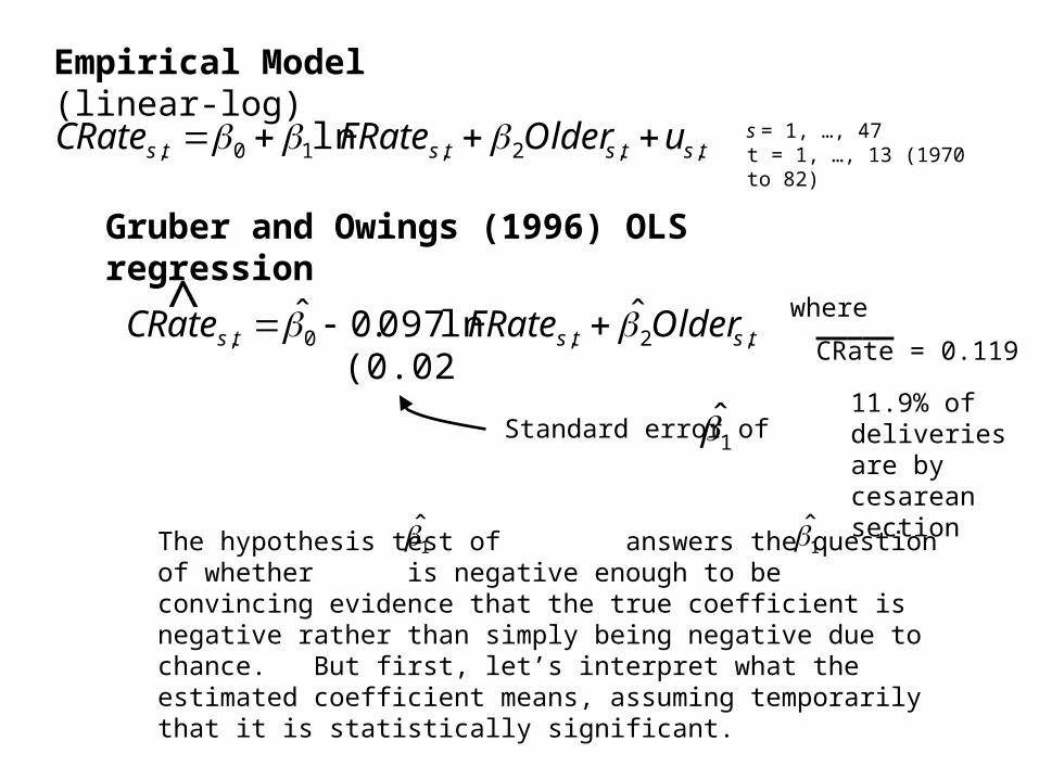
tstststs uOlderFRateCRate ,,2,10, ln s = 1, …, 47t = 1, …, 13 (1970 to 82)
Empirical Model (linear-log)
tststs OlderFRateCRate ,2,0,ˆln 097.0ˆ
Gruber and Owings (1996) OLS regression
1̂
^(0.021)
Standard error of
CRate = 0.119_____
where
11.9% of deliveries are by cesarean section
The hypothesis test of answers the question of whether is negative enough to be convincing evidence that the true coefficient is negative rather than simply being negative due to chance. But first, let’s interpret what the estimated coefficient means, assuming temporarily that it is statistically significant.
1̂ 1̂

Gruber and Owings interpretation of 1̂“A fall in the fertility rate of 10 percent is associated with an increase in the likelihood of cesarean delivery of 0.97 percentage points.” (p. 113)
00097.0100
097.0
100
ˆ
%1
FRate
CRate
What is the predicted effect of a 10% decrease in the fertility rate?
00097.010
CRate^%10097.0 CRate^ point

Set H0 and H1
H0: null hypothesis (straw man)
HA: alternative hypothesis (what we believe)
Does the empirical evidence convincingly knock H0 down?
Testing for demand inducement by obstetricians (OBs):
H0:
HA:
01 01
Gruber and Owings use economics to tell a story of why this might be true.
Two types of potential errorsTruth about β1
(OBs are guilty) (OBs are innocent)
no error Type I errorStatistical (OBs are guilty)
InferenceType II error no error
(OBs are innocent)
01
01
01
01

2i
ii2ˆ
)var(
))E((var11 PCig
uPCigPCig
ni
2
2i
2i
2i
2ˆ
)(1
ˆ)(2
11
ˆ1
PCigPCign
uPCigPCign
n
___
___
Hypothesis Testing of 1̂

Normally, a negative sign for is not sufficient to convince us to reject the null hypothesis and, in this case, conclude that OBs are guilty of inducing demand by carrying out unnecessary c-sections. Instead, has to be sufficient smaller than zero for us to be relatively confident that the true is negative. In other words, has to be smaller than some critical negative value, call it , for us to be willing to reject the null hypothesis.
1
1̂
1̂
C
Decision Rule
C 1̂
C 1̂
Find OBs
Do not Reject H0 Innocent
Reject H0 Guilty
1̂0 CReject H0 Accept H0
Prob (Type I error) = significance level of the test )N(0,~ˆ 2
ˆ11
Choose by setting Type I errorCReject true H0
Suppose 01

1̂0 C Reject H0 Accept H0
)N(0,~ˆ 2ˆ11
Given how would you illustrate the probability of making a Type II error? CType II error: accept a false H0.
Suppose 0*11
1̂0 *1C
Reject H0 Accept H0
),ˆN(~ˆ 2ˆ
*11
1Note: There is no way to measure Type II error without knowing the true value of
1

As the significance level of the test becomes more stringent, what happens to the prob(Type I error) and prob(Type II error)?
As prob(Type I error)
prob(Type II error)C
Given that changing the critical value decreases the probability of making one type of error while increasing the probability of making the other type of error, how should we set ? C
CSetting . Think about the cost of making each type of error.
prob(Type I error) reject true H0
prob(Type II error) accept false H0
• innocent OBs are tainted as demand inducers
• unnecessary policies may be introduced
• unnecessary c-sections

Typical practice set the significance level so that the probability of making at type I error is small.
Prob(Type I error ) is typically set at either .10, .05 or .01
But you should always question whether the typical practice is appropriate.
How do you find
1̂0 C
)N(0,~ˆ 2ˆ11
?C
One possibility: solve for whereC
05.0ˆd)N(0, 12ˆ1
C
Too cumbersome, requiring that we solve difficult problems for every new hypothesis.

How do you find ?C
Easier process: transform the test statistic into a standard normal one. Define z statistic as:
,1))ˆN(E(~)ˆE(ˆ
1ˆ
111
1
z
Standard normal distribution
But if H0 is true, then , so 0)ˆE( 1
N(0,1)~ˆ
1̂
11
z
1z0 Cz
)1N(0,~1zMuch easier a table of the standard normal distribution can be used to find the critical value for a variety of hypothesis tests.

BUT how do we calculate when is unknown? 1̂
11
ˆ
z1̂
Standard deviation of
1̂ˆ
1̂1̂
Solution substitute , which is the standard error of , for 1̂
)1(~ˆ
ˆ
ˆ
ˆ
11
0
ˆ
1
ˆ
H11
kntt
t distributiont statistic
n = Sample size
k+1= # parameters
The shape of the t distribution depends on the number of degrees of freedom. It is a little fatter than the standard normal distribution due to the increased variation of estimating .ˆwith
11ˆˆ

)1(~ˆ
ˆ
ˆ
ˆ
11
0
ˆ
1
ˆ
H11
kntt
Decision Rule ,Hreject then sign,right thehas ˆ& tt if 01C1 it.reject not do otherwise
The critical value, tC , depends on
1. Whether it is a one-sided or two-sided test.
2. The significance level of the test (usually, either 0.10, 0.05 or 0.01.
3. The degrees of freedom (n-k-1)