hysteresis models otani
TRANSCRIPT
1
Chapter 11. Member Hysteresis Models 11.1 Introduction
An inelastic earthquake response analysis of structures requires realistic hysteresis models, which can represent resistance-deformation relationship of a structural member model.
The resistance-deformation relations are different for constitutive materials of a section, for a section, for a member, for a story and for an entire structure. The resistance-deformation relation of a structural analysis unit observed in a laboratory test must be idealized into a resistance-deformation hysteresis model. Different levels of resistance-deformation models must be used for structural elements considered in an analysis; e.g., a constitutive model of materials in a finite element method analysis, a hysteresis model for a rotational spring in a one-component member model, a story shear-drift hysteresis model for a mass-spring model.
A hysteresis model is derived by extracting common features of resistance-deformation relations observed in laboratory tests of members of similar properties. The hysteresis model of a member must be able to express resistance-deformation relations under any loading history, including load reversals.
Resistance-deformation relationship under monotonically increasing loading is called the primary curve, skeleton curve or backbone curve. The skeleton curve provides an envelope of the hysteresis resistance-deformation relationship if the behavior is governed by stable flexure. The skeleton curve for reinforced concrete member is normally represented by a trilinear relation with stiffness changes at flexural cracking and tensile yielding of longitudinal reinforcement. The skeleton curve of a member must be defined on the basis of mechanical properties of constitutive materials and geometry of the member. Some researchers suggest the use of a bilinear relation with a stiffness change at yielding, ignoring the initial uncracked stage, because a reinforced concrete member subjected to light axial force can be easily cracked by shrinkage or accidental and gravity loading.
The state-of-the-art does not provide a reliable method to estimate the initial stiffness, yield
deformation and ultimate deformation. The stiffness degrades from the initial elastic stiffness with increased inelastic deformation and the number of cycles under reversed loading. The elastic modulus of concrete varies significantly with concrete strength and mix; initial cracks cause decay in the stiffness. The estimate of yield deformation is more complicated by the interaction of bending and shear deformation and additional deformation due to pullout of longitudinal reinforcement from the anchorage zone and due to bar slip of longitudinal reinforcement along the longitudinal reinforcement within the member. Empirical expressions are necessary for the estimate of yield and ultimate deformation.
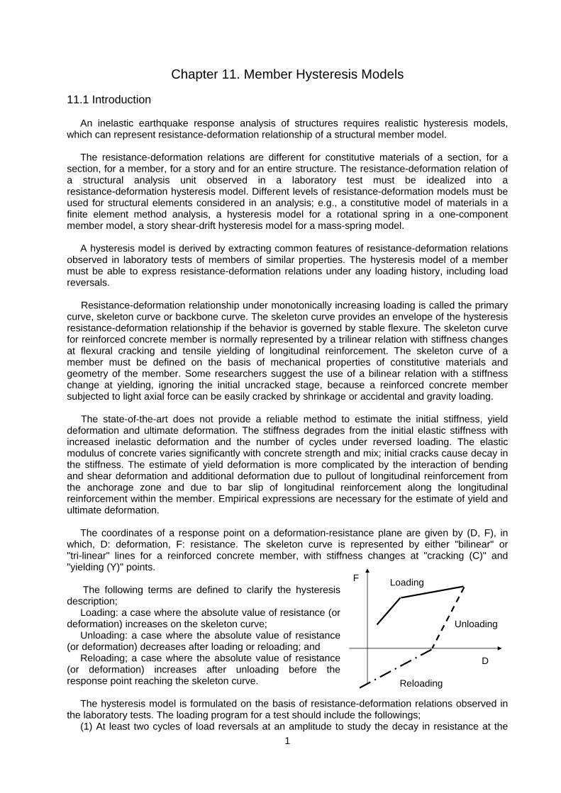
The coordinates of a response point on a deformation-resistance plane are given by (D, F), in which, D: deformation, F: resistance. The skeleton curve is represented by either "bilinear" or "tri-linear" lines for a reinforced concrete member, with stiffness changes at "cracking (C)" and "yielding (Y)" points.
The following terms are defined to clarify the hysteresis
description; Loading: a case where the absolute value of resistance (or
deformation) increases on the skeleton curve; Unloading: a case where the absolute value of resistance
(or deformation) decreases after loading or reloading; and Reloading; a case where the absolute value of resistance
(or deformation) increases after unloading before the response point reaching the skeleton curve.
The hysteresis model is formulated on the basis of resistance-deformation relations observed in
the laboratory tests. The loading program for a test should include the followings; (1) At least two cycles of load reversals at an amplitude to study the decay in resistance at the
Loading
Unloading
Reloading
D
F
2
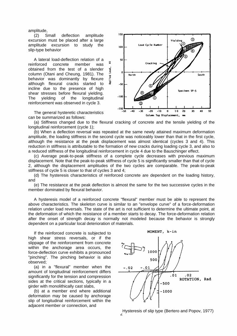
amplitude, (2) Small deflection amplitude
excursion must be placed after a large amplitude excursion to study the slip-type behavior
A lateral load-deflection relation of a reinforced concrete member was obtained from the test of a slender column (Otani and Cheung, 1981). The behavior was dominantly by flexure although flexural cracks started to incline due to the presence of high shear stresses before flexural yielding. The yielding of the longitudinal reinforcement was observed in cycle 3.
The general hysteretic characteristics
can be summarized as follows: (a) Stiffness changed due to the flexural cracking of concrete and the tensile yielding of the
longitudinal reinforcement (cycle 1); (b) When a deflection reversal was repeated at the same newly attained maximum deformation
amplitude, the loading stiffness in the second cycle was noticeably lower than that in the first cycle, although the resistance at the peak displacement was almost identical (cycles 3 and 4). This reduction in stiffness is attributable to the formation of new cracks during loading cycle 3, and also to a reduced stiffness of the longitudinal reinforcement in cycle 4 due to the Bauschinger effect.
(c) Average peak-to-peak stiffness of a complete cycle decreases with previous maximum displacement. Note that the peak-to-peak stiffness of cycle 5 is significantly smaller than that of cycle 2, although the displacement amplitudes of the two cycles are comparable. The peak-to-peak stiffness of cycle 5 is closer to that of cycles 3 and 4;
(d) The hysteresis characteristics of reinforced concrete are dependent on the loading history, and
(e) The resistance at the peak deflection is almost the same for the two successive cycles in the member dominated by flexural behavior.
A hysteresis model of a reinforced concrete "flexural" member must be able to represent the above characteristics. The skeleton curve is similar to an "envelope curve" of a force-deformation relation under load reversals. The state of the art is not sufficient to determine the ultimate point, at the deformation of which the resistance of a member starts to decay. The force-deformation relation after the onset of strength decay is normally not modeled because the behavior is strongly dependent on a particular local deterioration of materials.
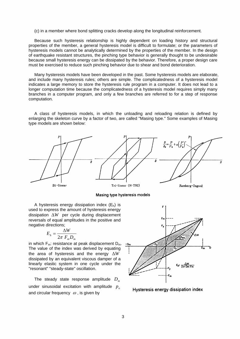
If the reinforced concrete is subjected to high shear stress reversals, or if the slippage of the reinforcement from concrete within the anchorage area occurs, the force-deflection curve exhibits a pronounced "pinching". The pinching behavior is also observed;
(a) in a "flexural" member when the amount of longitudinal reinforcement differs significantly for the tension and compression sides at the critical sections, typically in a girder with monolithically cast slabs,
(b) at a member end where additional deformation may be caused by anchorage slip of longitudinal reinforcement within the adjacent member or connection, and
Hysteresis of slip type (Bertero and Popov, 1977)
3
(c) in a member where bond splitting cracks develop along the longitudinal reinforcement.
Because such hysteresis relationship is highly dependent on loading history and structural properties of the member, a general hysteresis model is difficult to formulate; or the parameters of hysteresis models cannot be analytically determined by the properties of the member. In the design of earthquake resistant structures, the pinching type behavior is generally thought to be undesirable because small hysteresis energy can be dissipated by the behavior. Therefore, a proper design care must be exercised to reduce such pinching behavior due to shear and bond deterioration.
Many hysteresis models have been developed in the past. Some hysteresis models are elaborate, and include many hysteresis rules; others are simple. The complicatedness of a hysteresis model indicates a large memory to store the hysteresis rule program in a computer. It does not lead to a longer computation time because the complicatedness of a hysteresis model requires simply many branches in a computer program, and only a few branches are referred to for a step of response computation.
A class of hysteresis models, in which the unloading and reloading relation is defined by enlarging the skeleton curve by a factor of two, are called "Masing type." Some examples of Masing type models are shown below:
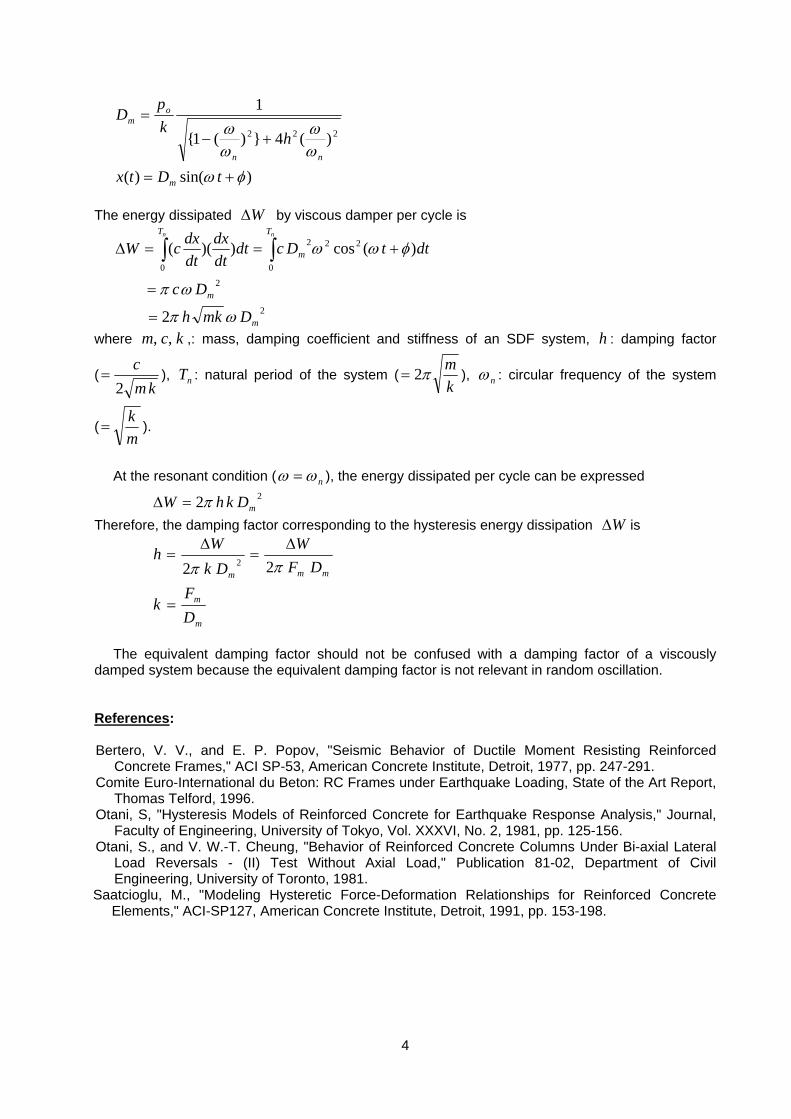
A hysteresis energy dissipation index (Eh) is
used to express the amount of hysteresis energy dissipation WΔ per cycle during displacement reversals of equal amplitudes in the positive and negative directions;
mm
h DFWE
π2Δ
=
in which Fm: resistance at peak displacement Dm. The value of the index was derived by equating the area of hysteresis and the energy WΔ dissipated by an equivalent viscous damper of a linearly elastic system in one cycle under the "resonant" "steady-state" oscillation.
The steady state response amplitude mD
under sinusoidal excitation with amplitude op and circular frequency ω , is given by
Hysteresis energy dissipation index
4
)sin()(
)(4})(1{
1
222
φωωω
ωω
+=
+−=
tDtx
hkp
D
m
nn
om
The energy dissipated WΔ by viscous damper per cycle is
2
2
22
0 0
2
2
)(cos))((
m
m
T T
m
Dmkh
Dc
dttDcdtdtdx
dtdxcW
n n
ωπ
ωπ
φωω
=
=
+==Δ ∫ ∫
where kcm ,, ,: mass, damping coefficient and stiffness of an SDF system, h : damping factor
(km
c2
= ), nT : natural period of the system (kmπ2= ), nω : circular frequency of the system
(mk
= ).
At the resonant condition ( nωω = ), the energy dissipated per cycle can be expressed
22 mDkhW π=Δ Therefore, the damping factor corresponding to the hysteresis energy dissipation WΔ is
m
m
mmm
DF
k
DFW
DkW
h
=
Δ=
Δ=
ππ 22 2
The equivalent damping factor should not be confused with a damping factor of a viscously
damped system because the equivalent damping factor is not relevant in random oscillation. References: Bertero, V. V., and E. P. Popov, "Seismic Behavior of Ductile Moment Resisting Reinforced
Concrete Frames," ACI SP-53, American Concrete Institute, Detroit, 1977, pp. 247-291. Comite Euro-International du Beton: RC Frames under Earthquake Loading, State of the Art Report,
Thomas Telford, 1996. Otani, S, "Hysteresis Models of Reinforced Concrete for Earthquake Response Analysis," Journal,
Faculty of Engineering, University of Tokyo, Vol. XXXVI, No. 2, 1981, pp. 125-156. Otani, S., and V. W.-T. Cheung, "Behavior of Reinforced Concrete Columns Under Bi-axial Lateral
Load Reversals - (II) Test Without Axial Load," Publication 81-02, Department of Civil Engineering, University of Toronto, 1981.
Saatcioglu, M., "Modeling Hysteretic Force-Deformation Relationships for Reinforced Concrete Elements," ACI-SP127, American Concrete Institute, Detroit, 1991, pp. 153-198.
5
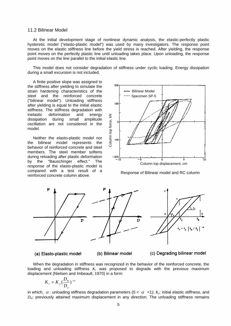
11.2 Bilinear Model
At the initial development stage of nonlinear dynamic analysis, the elastic-perfectly plastic hysteretic model ("elasto-plastic model") was used by many investigators. The response point moves on the elastic stiffness line before the yield stress is reached. After yielding, the response point moves on the perfectly plastic line until unloading takes place. Upon unloading, the response point moves on the line parallel to the initial elastic line.
This model does not consider degradation of stiffness under cyclic loading. Energy dissipation
during a small excursion is not included.
A finite positive slope was assigned to the stiffness after yielding to simulate the strain hardening characteristics of the steel and the reinforced concrete ("bilinear model"). Unloading stiffness after yielding is equal to the initial elastic stiffness. The stiffness degradation with inelastic deformation and energy dissipation during small amplitude oscillation are not considered in the model.
Neither the elasto-plastic model nor the bilinear model represents the behavior of reinforced concrete and steel members. The steel member softens during reloading after plastic deformation by the "Bauschinger effect." The response of the elasto-plastic model is compared with a test result of a reinforced concrete column above.
When the degradation in stiffness was recognized in the behavior of the reinforced concrete, the
loading and unloading stiffness Kr was proposed to degrade with the previous maximum displacement (Nielsen and Imbeault, 1970) in a form:
α−= )(y
myr D
DKK
in which, α : unloading stiffness degradation parameters (0 < α <1); Ky: initial elastic stiffness, and Dm: previously attained maximum displacement in any direction. The unloading stiffness remains
Bilinear ModelSpecimen SP-5
Column top displacement, cm
Col
umn
top
forc
e, k
N
Response of Bilinear model and RC column
6
constant until the response displacement amplitude exceeds the previous maximum displacement in either direction. The model is called a "degrading" bilinear hysteresis model." If the value of a is chosen to be zero, the unloading stiffness does not degrade with yielding. A smaller value of a tends to yield a larger residual displacement. The degrading bilinear model does not dissipate hysteretic energy until the yield is developed. For a reinforced concrete member, the value of α is normally selected to be around 0.4.
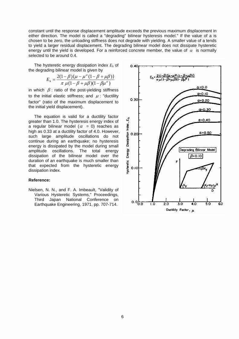
The hysteretic energy dissipation index Eh of the degrading bilinear model is given by
)1)(1()}1(){1(2
α
α
βμμββμπμββμμβ
−+−+−−−
=hE
in which β : ratio of the post-yielding stiffness to the initial elastic stiffness; and μ : "ductility factor" (ratio of the maximum displacement to the initial yield displacement).
The equation is valid for a ductility factor greater than 1.0. The hysteresis energy index of a regular bilinear model (α = 0) reaches as high as 0.33 at a ductility factor of 4.0. However, such large amplitude oscillations do not continue during an earthquake; no hysteresis energy is dissipated by the model during small amplitude oscillations. The total energy dissipation of the bilinear model over the duration of an earthquake is much smaller than that expected from the hysteretic energy dissipation index. Reference: Nielsen, N. N., and F. A. Imbeault, "Validity of
Various Hysteretic Systems," Proceedings, Third Japan National Conference on Earthquake Engineering, 1971, pp. 707-714.
7
11.3 Ramberg-Osgood Model
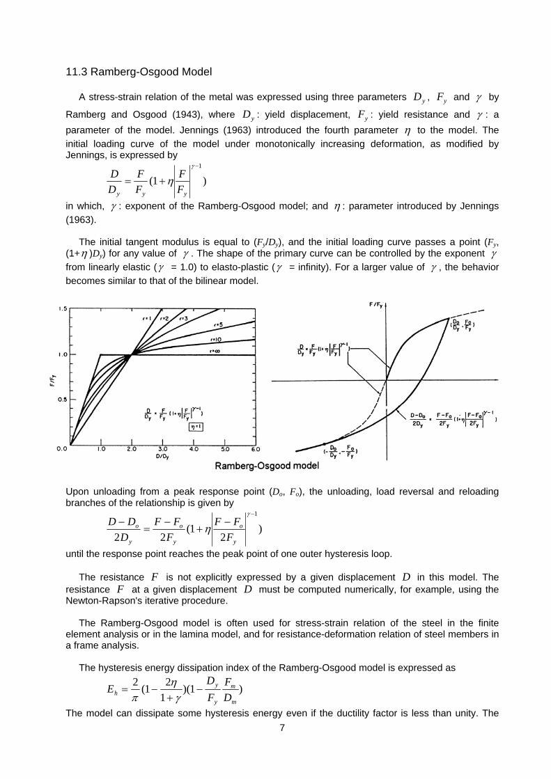
A stress-strain relation of the metal was expressed using three parameters yD , yF and γ by
Ramberg and Osgood (1943), where yD : yield displacement, yF : yield resistance and γ : a parameter of the model. Jennings (1963) introduced the fourth parameter η to the model. The initial loading curve of the model under monotonically increasing deformation, as modified by Jennings, is expressed by
)1(1−
+=γ
ηyyy F
FFF
DD
in which, γ : exponent of the Ramberg-Osgood model; and η : parameter introduced by Jennings (1963).
The initial tangent modulus is equal to (Fy/Dy), and the initial loading curve passes a point (Fy, (1+η )Dy) for any value of γ . The shape of the primary curve can be controlled by the exponent γ from linearly elastic (γ = 1.0) to elasto-plastic (γ = infinity). For a larger value of γ , the behavior becomes similar to that of the bilinear model.
Upon unloading from a peak response point (Do, Fo), the unloading, load reversal and reloading branches of the relationship is given by
)2
1(22
1−−
+−
=−
γ
ηy
o
y
o
y
o
FFF
FFF
DDD
until the response point reaches the peak point of one outer hysteresis loop.
The resistance F is not explicitly expressed by a given displacement D in this model. The resistance F at a given displacement D must be computed numerically, for example, using the Newton-Rapson's iterative procedure.
The Ramberg-Osgood model is often used for stress-strain relation of the steel in the finite element analysis or in the lamina model, and for resistance-deformation relation of steel members in a frame analysis.
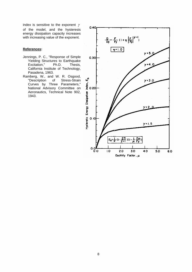
The hysteresis energy dissipation index of the Ramberg-Osgood model is expressed as
)1)(121(2
m
m
y
yh D
FFD
E −+
−=γη
π
The model can dissipate some hysteresis energy even if the ductility factor is less than unity. The
8
index is sensitive to the exponent γ of the model, and the hysteresis energy dissipation capacity increases with increasing value of the exponent. References: Jennings, P. C., "Response of Simple
Yielding Structures to Earthquake Excitation," Ph.D. Thesis, California Institute of Technology, Pasadena, 1963.
Ramberg, W., and W. R. Osgood, "Description of Stress-Strain Curves by Three Parameters," National Advisory Committee on Aeronautics, Technical Note 902, 1943.
9
11.4 Degrading Tri-linear Model
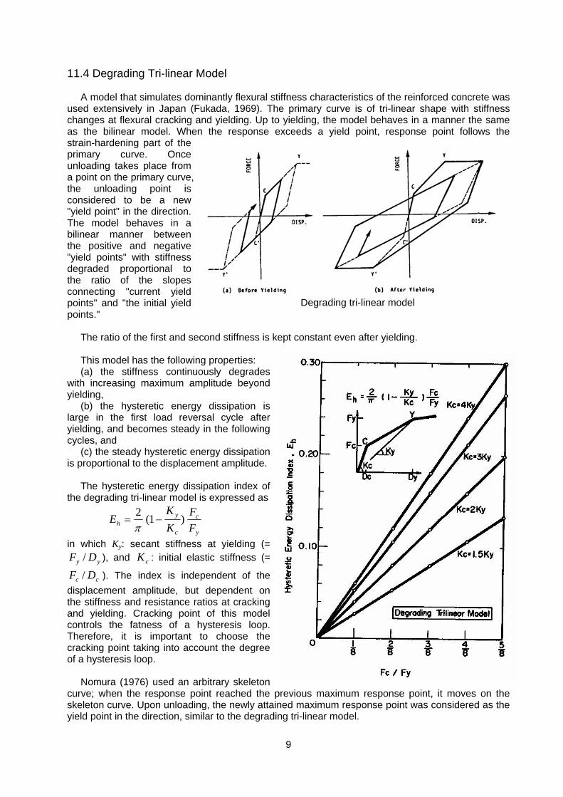
A model that simulates dominantly flexural stiffness characteristics of the reinforced concrete was used extensively in Japan (Fukada, 1969). The primary curve is of tri-linear shape with stiffness changes at flexural cracking and yielding. Up to yielding, the model behaves in a manner the same as the bilinear model. When the response exceeds a yield point, response point follows the strain-hardening part of the primary curve. Once unloading takes place from a point on the primary curve, the unloading point is considered to be a new "yield point" in the direction. The model behaves in a bilinear manner between the positive and negative "yield points" with stiffness degraded proportional to the ratio of the slopes connecting "current yield points" and "the initial yield points."
The ratio of the first and second stiffness is kept constant even after yielding.
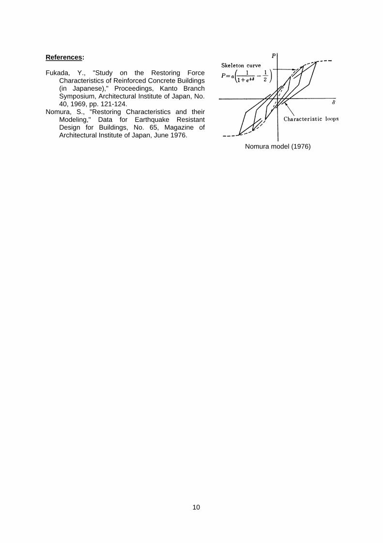
This model has the following properties: (a) the stiffness continuously degrades
with increasing maximum amplitude beyond yielding,
(b) the hysteretic energy dissipation is large in the first load reversal cycle after yielding, and becomes steady in the following cycles, and
(c) the steady hysteretic energy dissipation is proportional to the displacement amplitude.
The hysteretic energy dissipation index of the degrading tri-linear model is expressed as
y
c
c
yh F
FKK
E )1(2−=
π
in which Ky: secant stiffness at yielding (= yy DF / ), and cK : initial elastic stiffness (=
cc DF / ). The index is independent of the displacement amplitude, but dependent on the stiffness and resistance ratios at cracking and yielding. Cracking point of this model controls the fatness of a hysteresis loop. Therefore, it is important to choose the cracking point taking into account the degree of a hysteresis loop.
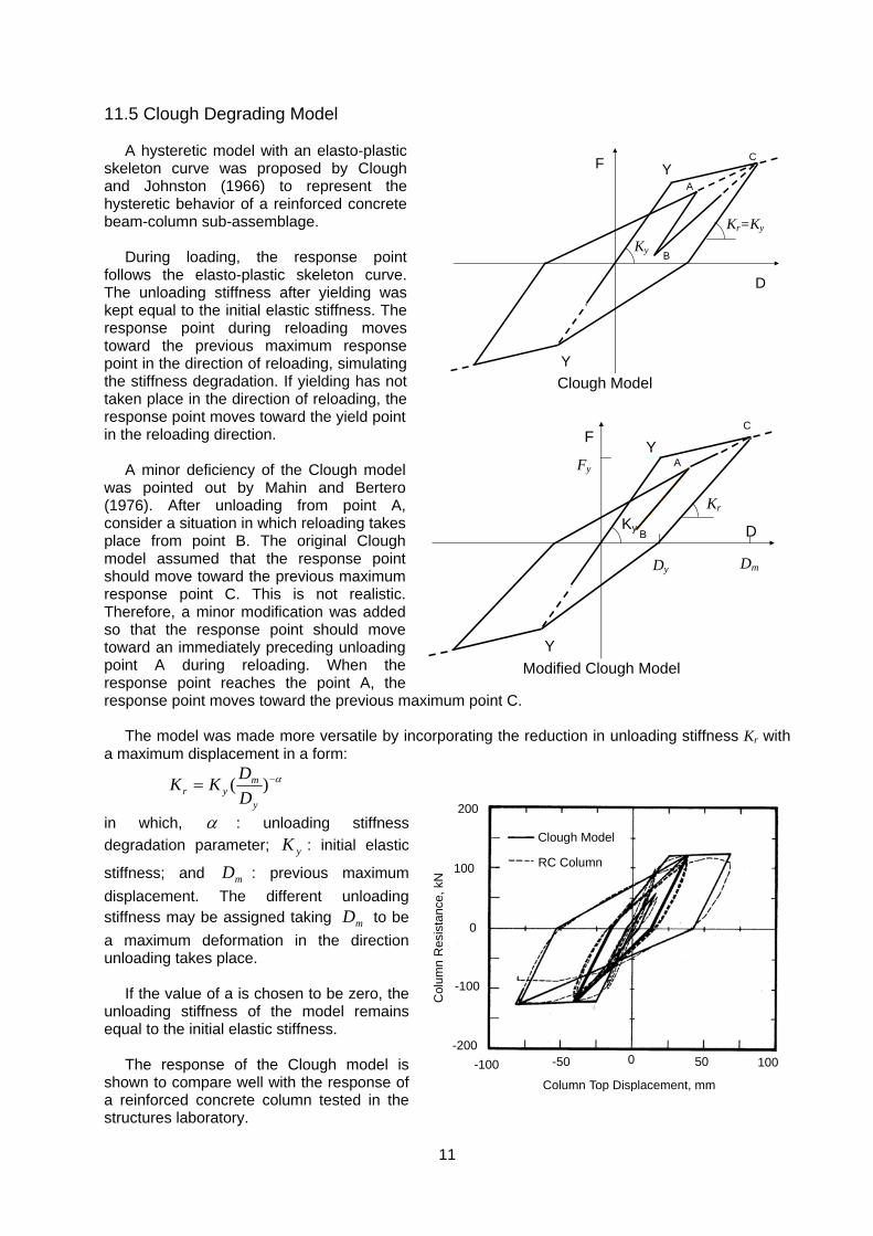
Nomura (1976) used an arbitrary skeleton curve; when the response point reached the previous maximum response point, it moves on the skeleton curve. Upon unloading, the newly attained maximum response point was considered as the yield point in the direction, similar to the degrading tri-linear model.
Degrading tri-linear model
10
References: Fukada, Y., "Study on the Restoring Force
Characteristics of Reinforced Concrete Buildings (in Japanese)," Proceedings, Kanto Branch Symposium, Architectural Institute of Japan, No. 40, 1969, pp. 121-124.
Nomura, S., "Restoring Characteristics and their Modeling," Data for Earthquake Resistant Design for Buildings, No. 65, Magazine of Architectural Institute of Japan, June 1976.
Nomura model (1976)
11
11.5 Clough Degrading Model
A hysteretic model with an elasto-plastic skeleton curve was proposed by Clough and Johnston (1966) to represent the hysteretic behavior of a reinforced concrete beam-column sub-assemblage.
During loading, the response point
follows the elasto-plastic skeleton curve. The unloading stiffness after yielding was kept equal to the initial elastic stiffness. The response point during reloading moves toward the previous maximum response point in the direction of reloading, simulating the stiffness degradation. If yielding has not taken place in the direction of reloading, the response point moves toward the yield point in the reloading direction.
A minor deficiency of the Clough model was pointed out by Mahin and Bertero (1976). After unloading from point A, consider a situation in which reloading takes place from point B. The original Clough model assumed that the response point should move toward the previous maximum response point C. This is not realistic. Therefore, a minor modification was added so that the response point should move toward an immediately preceding unloading point A during reloading. When the response point reaches the point A, the response point moves toward the previous maximum point C.
The model was made more versatile by incorporating the reduction in unloading stiffness Kr with a maximum displacement in a form:
α−= )(y
myr D
DKK
in which, α : unloading stiffness degradation parameter; yK : initial elastic
stiffness; and mD : previous maximum displacement. The different unloading stiffness may be assigned taking mD to be a maximum deformation in the direction unloading takes place.
If the value of a is chosen to be zero, the unloading stiffness of the model remains equal to the initial elastic stiffness.
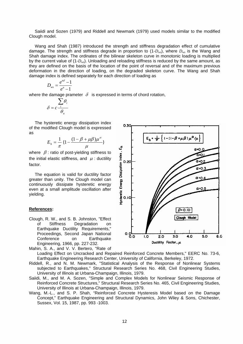
The response of the Clough model is
shown to compare well with the response of a reinforced concrete column tested in the structures laboratory.
Clough Model
RC Column
Column Top Displacement, mm
Col
umn
Res
ista
nce,
kN
-100 -50 0 50 100
100
200
0
-100
-200
D
F
B
CY
Y
Kr=Ky Ky
A
Clough Model
D
F
B
C
Y
Y
Kr Ky
Dm Dy
Fy A
Modified Clough Model
12
Saiidi and Sozen (1979) and Riddell and Newmark (1979) used models similar to the modified Clough model.
Wang and Shah (1987) introduced the strength and stiffness degradation effect of cumulative damage. The strength and stiffness degrade in proportion to (1-Dws), where Dws is the Wang and Shah damage index. The ordinates of the bilinear skeleton curve in monotonic loading is multiplied by the current value of (1-Dws). Unloading and reloading stiffness is reduced by the same amount, as they are defined on the basis of the location of the point of reversal and of the maximum previous deformation in the direction of loading, on the degraded skeleton curve. The Wang and Shah damage index is defined separately for each direction of loading as
11
n
ws n
eDe
δ −=
−
where the damage prameter δ is expressed in terms of chord rotation,
i
i
u
cθ
δθ
=∑
The hysteretic energy dissipation index
of the modified Clough model is expressed as
})1(1{1μ
μμββπ
α+−−=hE
where β : ratio of post-yielding stiffness to the initial elastic stiffness, and μ : ductility factor.
The equation is valid for ductility factor greater than unity. The Clough model can continuously dissipate hysteretic energy even at a small amplitude oscillation after yielding. References: Clough, R. W., and S. B. Johnston, "Effect
of Stiffness Degradation on Earthquake Ductility Requirements," Proceedings, Second Japan National Conference on Earthquake Engineering, 1966, pp. 227-232.
Mahin, S. A., and V. V. Bertero, "Rate of Loading Effect on Uncracked and Repaired Reinforced Concrete Members," EERC No. 73-6, Earthquake Engineering Research Center, University of California, Berkeley, 1972.
Riddell, R., and N. M. Newmark, "Statistical Analysis of the Response of Nonlinear Systems subjected to Earthquakes," Structural Research Series No. 468, Civil Engineering Studies, University of Illinois at Urbana-Champaign, Illinois, 1979.
Saiidi, M., and M. A. Sozen, "Simple and Complex Models for Nonlinear Seismic Response of Reinforced Concrete Structures," Structural Research Series No. 465, Civil Engineering Studies, University of Illinois at Urbana-Champaign, Illinois, 1979.
Wang, M.-L., and S. P. Shah, “Reinforced Concrete Hysteresis Model based on the Damage Concept,” Earthquake Engineering and Structural Dynamics, John Wiley & Sons, Chichester, Sussex, Vol. 15, 1987, pp. 993 -1003.
13
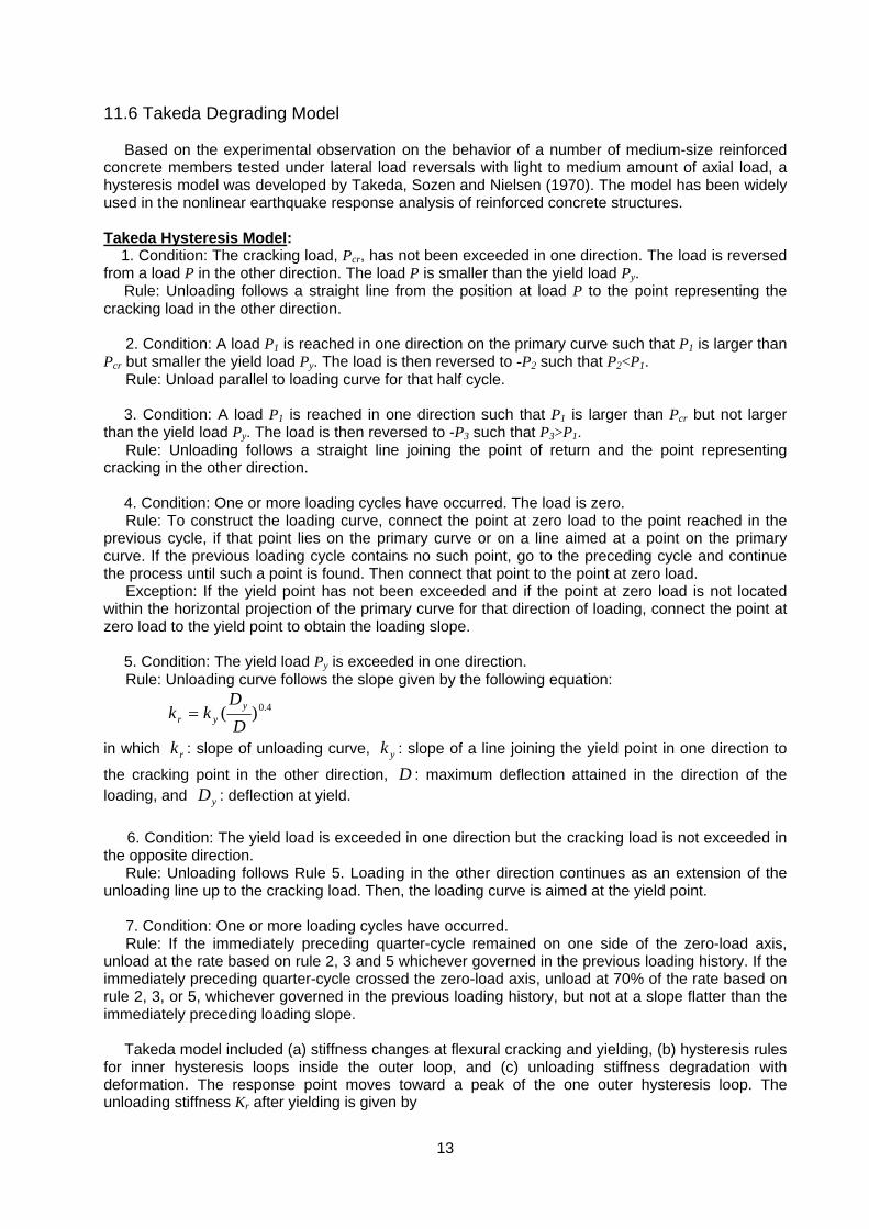
11.6 Takeda Degrading Model
Based on the experimental observation on the behavior of a number of medium-size reinforced concrete members tested under lateral load reversals with light to medium amount of axial load, a hysteresis model was developed by Takeda, Sozen and Nielsen (1970). The model has been widely used in the nonlinear earthquake response analysis of reinforced concrete structures. Takeda Hysteresis Model:
1. Condition: The cracking load, Pcr, has not been exceeded in one direction. The load is reversed from a load P in the other direction. The load P is smaller than the yield load Py.
Rule: Unloading follows a straight line from the position at load P to the point representing the cracking load in the other direction.
2. Condition: A load P1 is reached in one direction on the primary curve such that P1 is larger than
Pcr but smaller the yield load Py. The load is then reversed to -P2 such that P2<P1. Rule: Unload parallel to loading curve for that half cycle. 3. Condition: A load P1 is reached in one direction such that P1 is larger than Pcr but not larger
than the yield load Py. The load is then reversed to -P3 such that P3>P1. Rule: Unloading follows a straight line joining the point of return and the point representing
cracking in the other direction. 4. Condition: One or more loading cycles have occurred. The load is zero. Rule: To construct the loading curve, connect the point at zero load to the point reached in the
previous cycle, if that point lies on the primary curve or on a line aimed at a point on the primary curve. If the previous loading cycle contains no such point, go to the preceding cycle and continue the process until such a point is found. Then connect that point to the point at zero load.
Exception: If the yield point has not been exceeded and if the point at zero load is not located within the horizontal projection of the primary curve for that direction of loading, connect the point at zero load to the yield point to obtain the loading slope.
5. Condition: The yield load Py is exceeded in one direction. Rule: Unloading curve follows the slope given by the following equation:
4.0)(DD
kk yyr =
in which rk : slope of unloading curve, yk : slope of a line joining the yield point in one direction to
the cracking point in the other direction, D : maximum deflection attained in the direction of the loading, and yD : deflection at yield.
6. Condition: The yield load is exceeded in one direction but the cracking load is not exceeded in
the opposite direction. Rule: Unloading follows Rule 5. Loading in the other direction continues as an extension of the
unloading line up to the cracking load. Then, the loading curve is aimed at the yield point. 7. Condition: One or more loading cycles have occurred. Rule: If the immediately preceding quarter-cycle remained on one side of the zero-load axis,
unload at the rate based on rule 2, 3 and 5 whichever governed in the previous loading history. If the immediately preceding quarter-cycle crossed the zero-load axis, unload at 70% of the rate based on rule 2, 3, or 5, whichever governed in the previous loading history, but not at a slope flatter than the immediately preceding loading slope.
Takeda model included (a) stiffness changes at flexural cracking and yielding, (b) hysteresis rules for inner hysteresis loops inside the outer loop, and (c) unloading stiffness degradation with deformation. The response point moves toward a peak of the one outer hysteresis loop. The unloading stiffness Kr after yielding is given by
14
α−
++
=y
m
yc
ycr D
DDDFF
K
in which, α : unloading stiffness degradation parameter; and mD : previous maximum displacement beyond yielding in the direction concerned. The hysteresis rules are extensive and comprehensive.
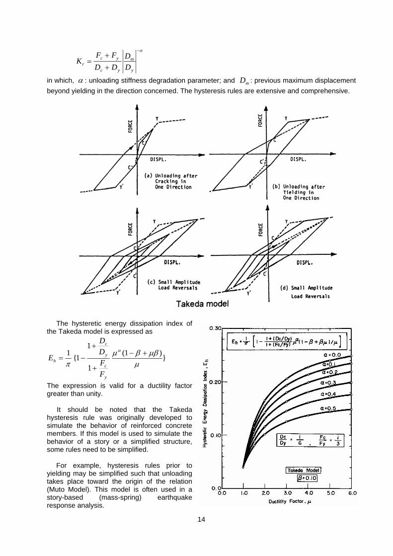
The hysteretic energy dissipation index of
the Takeda model is expressed as
})1(
1
11{1
μμββμ
π
α +−
+
+−=
y
c
y
c
h
FFDD
E
The expression is valid for a ductility factor greater than unity.
It should be noted that the Takeda hysteresis rule was originally developed to simulate the behavior of reinforced concrete members. If this model is used to simulate the behavior of a story or a simplified structure, some rules need to be simplified.
For example, hysteresis rules prior to yielding may be simplified such that unloading takes place toward the origin of the relation (Muto Model). This model is often used in a story-based (mass-spring) earthquake response analysis.
15
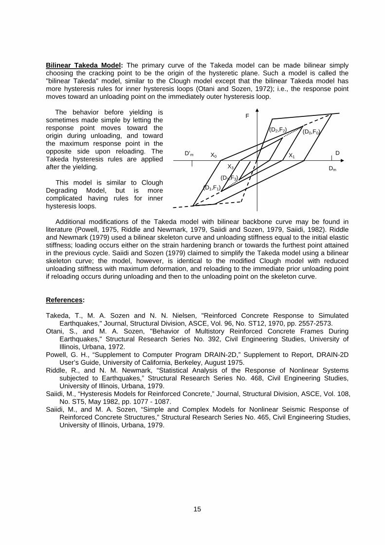
Bilinear Takeda Model: The primary curve of the Takeda model can be made bilinear simply choosing the cracking point to be the origin of the hysteretic plane. Such a model is called the "bilinear Takeda" model, similar to the Clough model except that the bilinear Takeda model has more hysteresis rules for inner hysteresis loops (Otani and Sozen, 1972); i.e., the response point moves toward an unloading point on the immediately outer hysteresis loop.
The behavior before yielding is sometimes made simple by letting the response point moves toward the origin during unloading, and toward the maximum response point in the opposite side upon reloading. The Takeda hysteresis rules are applied after the yielding.
This model is similar to Clough Degrading Model, but is more complicated having rules for inner hysteresis loops.
Additional modifications of the Takeda model with bilinear backbone curve may be found in literature (Powell, 1975, Riddle and Newmark, 1979, Saiidi and Sozen, 1979, Saiidi, 1982). Riddle and Newmark (1979) used a bilinear skeleton curve and unloading stiffness equal to the initial elastic stiffness; loading occurs either on the strain hardening branch or towards the furthest point attained in the previous cycle. Saiidi and Sozen (1979) claimed to simplify the Takeda model using a bilinear skeleton curve; the model, however, is identical to the modified Clough model with reduced unloading stiffness with maximum deformation, and reloading to the immediate prior unloading point if reloading occurs during unloading and then to the unloading point on the skeleton curve. References: Takeda, T., M. A. Sozen and N. N. Nielsen, "Reinforced Concrete Response to Simulated
Earthquakes," Journal, Structural Division, ASCE, Vol. 96, No. ST12, 1970, pp. 2557-2573. Otani, S., and M. A. Sozen, "Behavior of Multistory Reinforced Concrete Frames During
Earthquakes," Structural Research Series No. 392, Civil Engineering Studies, University of Illinois, Urbana, 1972.
Powell, G. H., “Supplement to Computer Program DRAIN-2D,” Supplement to Report, DRAIN-2D User’s Guide, University of California, Berkeley, August 1975.
Riddle, R., and N. M. Newmark, “Statistical Analysis of the Response of Nonlinear Systems subjected to Earthquakes,” Structural Research Series No. 468, Civil Engineering Studies, University of Illinois, Urbana, 1979.
Saiidi, M., “Hysteresis Models for Reinforced Concrete,” Journal, Structural Division, ASCE, Vol. 108, No. ST5, May 1982, pp. 1077 - 1087.
Saiidi, M., and M. A. Sozen, “Simple and Complex Models for Nonlinear Seismic Response of Reinforced Concrete Structures,” Structural Research Series No. 465, Civil Engineering Studies, University of Illinois, Urbana, 1979.
D
F
Dm
D’m X0
(D0,F0)
X1
(D1,F1)
X3
(D2,F2)
(D3,F3)
16
11.7 Pivot Model
Major features of the force-deflection hysteresis results of large-scale reinforced concrete members are;
(1) Unloading stiffness decreases as displacement ductility increases,
(2) Following a nonlinear excursion in one direction, upon load reversal, the force-deflection path crosses the idealized initial stiffness line prior to reaching the idealized yield force, and
(3) The effect of pre-cracked stiffness may be ignored. The use of the pivot point in defining degraded unloading stiffness was first proposed by Kunnath et al. (1990).
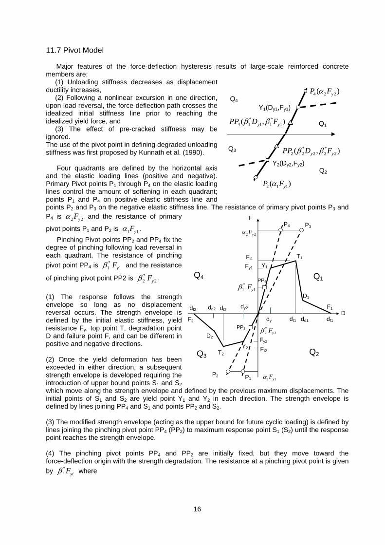
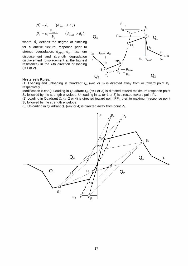
Four quadrants are defined by the horizontal axis and the elastic loading lines (positive and negative). Primary Pivot points P1 through P4 on the elastic loading lines control the amount of softening in each quadrant; points P1 and P4 on positive elastic stiffness line and points P2 and P3 on the negative elastic stiffness line. The resistance of primary pivot points P3 and P4 is 2 2yFα and the resistance of primary
pivot points P1 and P2 is 1 1yFα . Pinching Pivot points PP2 and PP4 fix the
degree of pinching following load reversal in each quadrant. The resistance of pinching pivot point PP4 is *
1 1yFβ and the resistance
of pinching pivot point PP2 is *2 2yFβ .
(1) The response follows the strength envelope so long as no displacement reversal occurs. The strength envelope is defined by the initial elastic stiffness, yield resistance Fy, top point T, degradation point D and failure point F, and can be different in positive and negative directions. (2) Once the yield deformation has been exceeded in either direction, a subsequent strength envelope is developed requiring the introduction of upper bound points S1 and S2 which move along the strength envelope and defined by the previous maximum displacements. The initial points of S1 and S2 are yield point Y1 and Y2 in each direction. The strength envelope is defined by lines joining PP4 and S1 and points PP2 and S2. (3) The modified strength envelope (acting as the upper bound for future cyclic loading) is defined by lines joining the pinching pivot point PP4 (PP2) to maximum response point S1 (S2) until the response point reaches the strength envelope. (4) The pinching pivot points PP4 and PP2 are initially fixed, but they move toward the force-deflection origin with the strength degradation. The resistance at a pinching pivot point is given by *
i yiFβ where
Q1
Q2
Q3
Q44 2 2( )yP Fα
2 1 1( )yP Fα
Y2(Dy2,Fy2)
Y1(Dy1,Fy1) * *
4 1 1 1 1( , )y yPP D Fβ β
* *2 2 2 2 2( , )y yPP D Fβ β
Q1
Q2
Q4
Q3
D
F
Y1
Y2
P1
P4 P3
P2
dy dt1 dd1 df1
Fy1
Fy2
dy2
2 2yFα
1 1yFα
dt2dd2df2
PP4
PP2
Ft1
Ft2
D1
T1
F1
T2
D2
F2
*1 1yFβ
*2 2yFβ
17
)(
)(
*
*
tiiMAXti
iMAXii
tiiMAXii
ddF
Fdd
>=
≤=
ββ
ββ
where iβ defines the degree of pinching for a ductile flexural response prior to strength degradation. tiiMAX dd , : maximum displacement and strength degradation displacement (displacement at the highest resistance) in the i-th direction of loading (i=1 or 2). Hysteresis Rules: (1) Loading and unloading in Quadrant Qn (n=1 or 3) is directed away from or toward point Pn, respectively. Modification (Otani): Loading in Quadrant Qn (n=1 or 3) is directed toward maximum response point Si, followed by the strength envelope. Unloading in Qn (n=1 or 3) is directed toward point Pn. (2) Loading in Quadrant Qn (n=2 or 4) is directed toward point PPn, then to maximum response point Si, followed by the strength envelope. (3) Unloading in Quadrant Qn (n=2 or 4) is directed away from point Pn.
Q1
Q2
Q4
Q3
D
F
Y1
Y2
P1
P4 P3
P2
PP4
PP2
S1
S2
Q1
Q2
Q4
Q3
D
F
Y1
Y2
dt1 df1
dt2df2
PP4
PP2
D1
T1
F1
T2
D2
F2
S1
S2
D1MAX
D2MAX
F2MAX
F1MAX
Ft2
Ft1
18
Modification for Softened Initial Stiffness: The unlading stiffness of the maximum
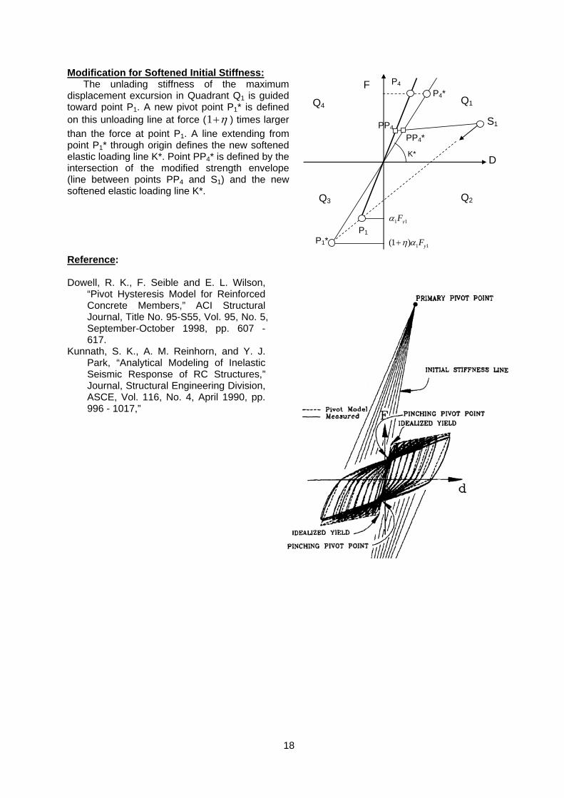
displacement excursion in Quadrant Q1 is guided toward point P1. A new pivot point P1* is defined on this unloading line at force (1 η+ ) times larger than the force at point P1. A line extending from point P1* through origin defines the new softened elastic loading line K*. Point PP4* is defined by the intersection of the modified strength envelope (line between points PP4 and S1) and the new softened elastic loading line K*. Reference: Dowell, R. K., F. Seible and E. L. Wilson,
“Pivot Hysteresis Model for Reinforced Concrete Members,” ACI Structural Journal, Title No. 95-S55, Vol. 95, No. 5, September-October 1998, pp. 607 - 617.
Kunnath, S. K., A. M. Reinhorn, and Y. J. Park, “Analytical Modeling of Inelastic Seismic Response of RC Structures,” Journal, Structural Engineering Division, ASCE, Vol. 116, No. 4, April 1990, pp. 996 - 1017,”
Q2 Q3
Q4 Q1
S1
D
PP4
PP4*
1 1yFα
1 1(1 ) yFη α+ P1
P1*
F P4 P4*
K*
19
Pivot Hysteresis Model (Version 2) Reference: Dowell, R. K., F. Seible and E. L. Wilson, "Pivot Hysteresis Model for Reinforced Concrete
Members," ACI Structural Journal, Title No. 95-S55, Vol. 95, No. 5, September-October 1998, pp. 607 - 617.
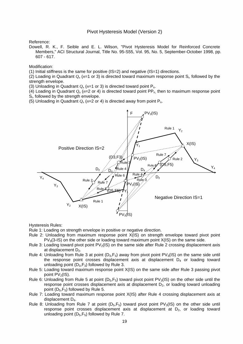
Modification: (1) Initial stiffness is the same for positive (IS=2) and negative (IS=1) directions. (2) Loading in Quadrant Qn (n=1 or 3) is directed toward maximum response point Si, followed by the strength envelope. (3) Unloading in Quadrant Qn (n=1 or 3) is directed toward point Pn. (4) Loading in Quadrant Qn (n=2 or 4) is directed toward point PPn, then to maximum response point Si, followed by the strength envelope. (5) Unloading in Quadrant Qn (n=2 or 4) is directed away from point Pn.
Hysteresis Rules: Rule 1: Loading on strength envelope in positive or negative direction. Rule 2: Unloading from maximum response point X(IS) on strength envelope toward pivot point
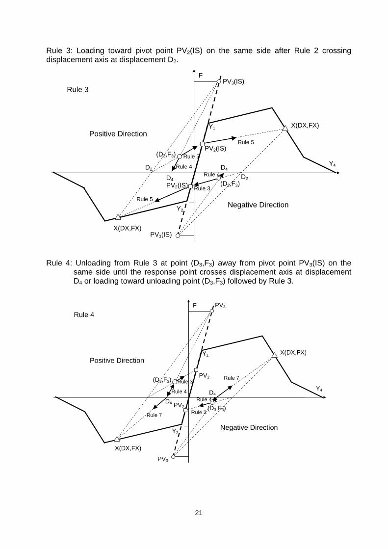
PV3(3-IS) on the other side or loading toward maximum point X(IS) on the same side. Rule 3: Loading toward pivot point PV2(IS) on the same side after Rule 2 crossing displacement axis
at displacement D2. Rule 4: Unloading from Rule 3 at point (D3,F3) away from pivot point PV3(IS) on the same side until
the response point crosses displacement axis at displacement D4 or loading toward unloading point (D3,F3) followed by Rule 3.
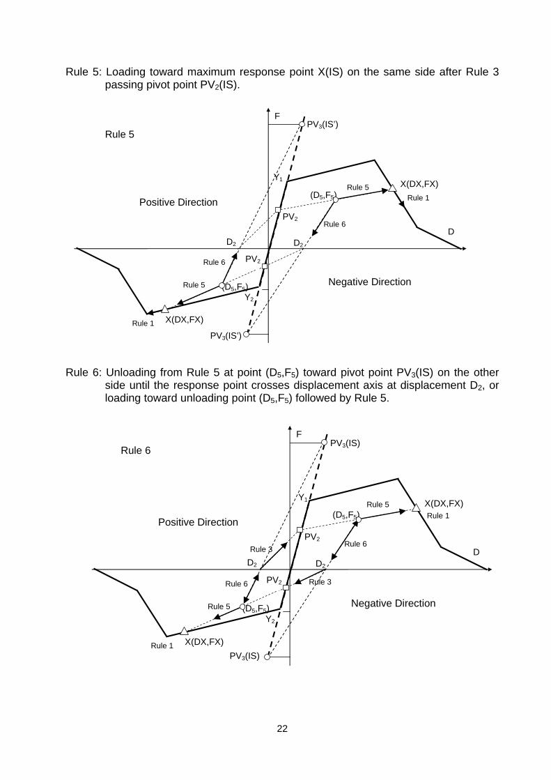
Rule 5: Loading toward maximum response point X(IS) on the same side after Rule 3 passing pivot point PV2(IS).
Rule 6: Unloading from Rule 5 at point (D5,F5) toward pivot point PV3(IS) on the other side until the response point crosses displacement axis at displacement D2, or loading toward unloading point (D5,F5) followed by Rule 5.
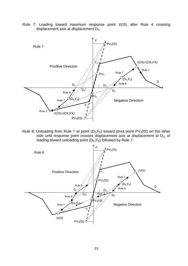
Rule 7: Loading toward maximum response point X(IS) after Rule 4 crossing displacement axis at displacement D4.
Rule 8: Unloading from Rule 7 at point (D5,F5) toward pivot point PV3(IS) on the other side until response point crosses displacement axis at displacement at D2, or loading toward unloading point (D5,F5) followed by Rule 7.
Y4
F
Y1
Y1
PV3(IS)
PV3(IS)
PV2(IS)
PV2(IS)
X(IS)
X(IS)
Rule 1
Rule 2
D2Rule 3Rule 4
Rule 5
Rule 2
Rule 3
Rule 4 D4
Rule 7
Rule 7
Rule 6
Y2
Y3
Y2
Y3
Y4
Rule 1
Rule 8
Negative Direction IS=1
Positive Direction IS=2
D2
(D3,F3)
D4
(D5,F5)
(D5,F5)
20
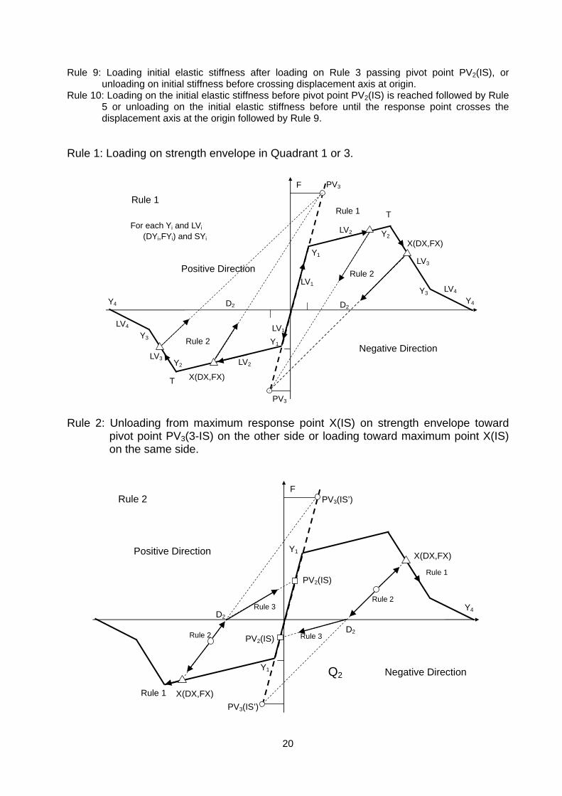
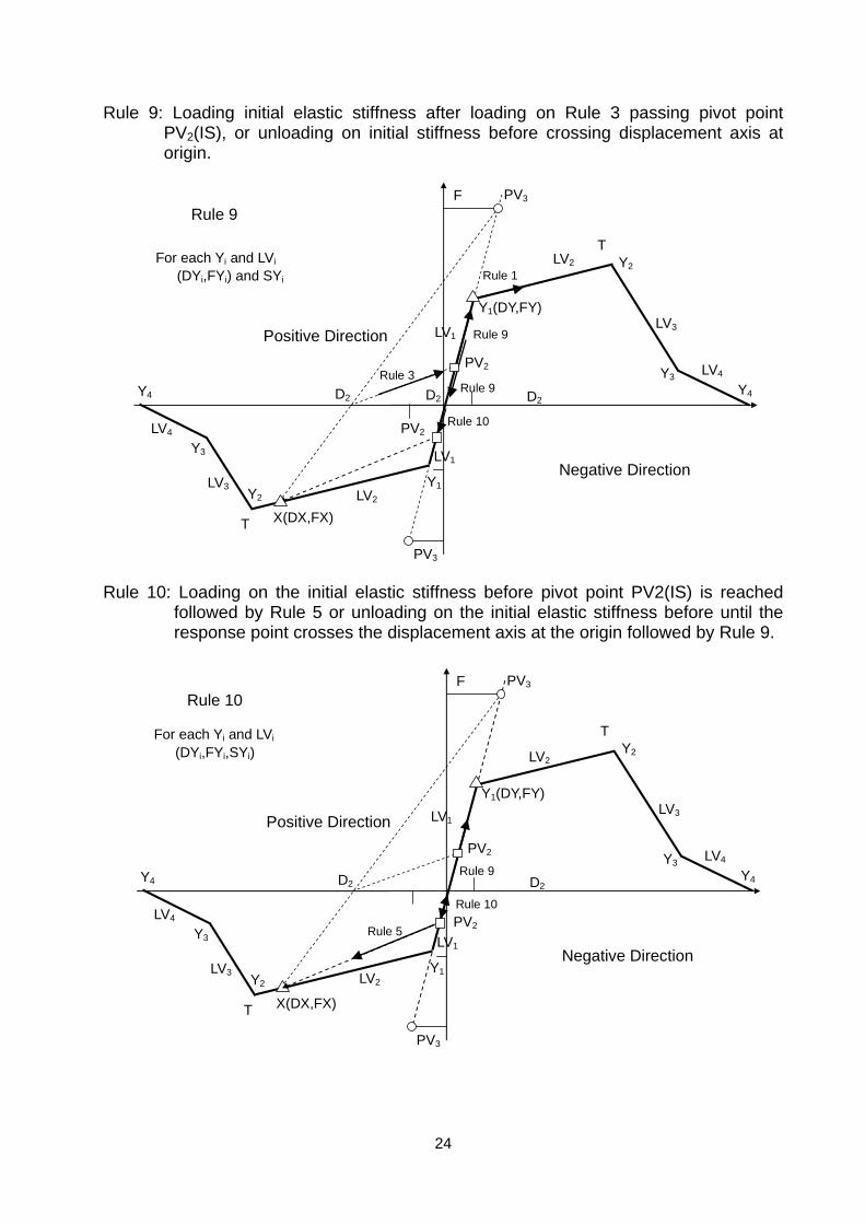
Rule 9: Loading initial elastic stiffness after loading on Rule 3 passing pivot point PV2(IS), or unloading on initial stiffness before crossing displacement axis at origin.
Rule 10: Loading on the initial elastic stiffness before pivot point PV2(IS) is reached followed by Rule 5 or unloading on the initial elastic stiffness before until the response point crosses the displacement axis at the origin followed by Rule 9.
Rule 1: Loading on strength envelope in Quadrant 1 or 3.
Rule 2: Unloading from maximum response point X(IS) on strength envelope toward
pivot point PV3(3-IS) on the other side or loading toward maximum point X(IS) on the same side.
F
Y1
Y3
PV3
PV3
X(DX,FX)
X(DX,FX)
Rule 1 T
T
LV1
LV2
LV3
LV4
Y2
Y3 Y4
Y1
Y2
LV1
LV2LV3
LV4
For each Yi and LVi (DYi,FYi) and SYi
Rule 2
Rule 2
D2D2Y4
Negative Direction
Positive Direction
Rule 1
Q2
Y4
F
Y1
Y1
PV3(IS’)
PV3(IS’)
PV2(IS)
PV2(IS)
X(DX,FX)
X(DX,FX)
Rule 1
Rule 2
D2Rule 3Rule 2
Rule 3D2
Negative Direction
Positive Direction
Rule 1
Rule 2
21
Rule 3: Loading toward pivot point PV2(IS) on the same side after Rule 2 crossing displacement axis at displacement D2.
Rule 4: Unloading from Rule 3 at point (D3,F3) away from pivot point PV3(IS) on the
same side until the response point crosses displacement axis at displacement D4 or loading toward unloading point (D3,F3) followed by Rule 3.
Y4
F
Y1
Y2
PV3(IS)
PV3(IS)
PV2(IS)
PV2(IS)
X(DX,FX)
X(DX,FX)
D2
Rule 3
Rule 4
Rule 3
Rule 4 D4
D4
D2
(D3,F3)
(D3,F3)
Negative Direction
Positive Direction Rule 5
Rule 5
Rule 3
Y4
F
Y1
Y2
PV3
PV3
PV2
PV2
X(DX,FX)
X(DX,FX)
Rule 3
Rule 4
Rule 3
Rule 4 D4
D4(D3,F3)
(D3,F3) Rule 7
Rule 7
Negative Direction
Positive Direction
Rule 4
22
Rule 5: Loading toward maximum response point X(IS) on the same side after Rule 3 passing pivot point PV2(IS).
Rule 6: Unloading from Rule 5 at point (D5,F5) toward pivot point PV3(IS) on the other
side until the response point crosses displacement axis at displacement D2, or loading toward unloading point (D5,F5) followed by Rule 5.
D
F
Y1
Y2
PV3(IS’)
PV3(IS’)
PV2
PV2
X(DX,FX)
X(DX,FX)
Rule 5
Rule 5
Rule 6
Rule 6
Rule 1
Rule 1 (D5,F5)
(D5,F5)
D2D2
Negative Direction
Positive Direction
Rule 5
D
F
Y1
Y2
PV3(IS)
PV3(IS)
PV2
PV2
X(DX,FX)
X(DX,FX)
Rule 5
Rule 5
Rule 6
Rule 6
Rule 1
Rule 1 (D5,F5)
(D5,F5)
D2D2
Negative Direction
Positive Direction
Rule 3
Rule 3
Rule 6
23
Rule 7: Loading toward maximum response point X(IS) after Rule 4 crossing displacement axis at displacement D4.
Rule 8: Unloading from Rule 7 at point (D5,F5) toward pivot point PV3(IS) on the other
side until response point crosses displacement axis at displacement at D2, or loading toward unloading point (D5,F5) followed by Rule 7.
D
F
Y1
Y1
PV3(IS)
PV3(IS)
PV2(IS)
PV2(IS)
X(IS)
X(IS)
Rule 3
Rule 3
D4
D4
Rule 7
Rule 7
(D5,F5)
D2
(D5,F5)
Rule 8
Rule 8
D2
Negative Direction
Positive Direction
Rule 8
D
F
Y1
Y1
PV3(IS)
PV3(IS)
PV2
PV2
X(IS)=(DX,FX)
X(IS)=(DX,FX)
D4
D4
Rule 7
Rule 7
(D5,F5)
D2
(D5,F5)
Rule 6
Rule 6
D2
Negative Direction
Positive Direction
Rule 1
Rule 1
Rule 7
24
Rule 9: Loading initial elastic stiffness after loading on Rule 3 passing pivot point PV2(IS), or unloading on initial stiffness before crossing displacement axis at origin.
Rule 10: Loading on the initial elastic stiffness before pivot point PV2(IS) is reached
followed by Rule 5 or unloading on the initial elastic stiffness before until the response point crosses the displacement axis at the origin followed by Rule 9.
F
Y3
PV3
PV3
Y1(DY,FY)
X(DX,FX)
Rule 9
T
T
LV1
LV2
LV3
LV4
Y2
Y3 Y4
Y1Y2
LV1
LV2LV3
LV4
For each Yi and LVi (DYi,FYi) and SYi
D2D2 Y4
Negative Direction
Positive Direction
Rule 3PV2
Rule 9
Rule 9
PV2Rule 10
D2
Rule 1
F
Y3
PV3
PV3
Y1(DY,FY)
X(DX,FX)
Rule 10
T
T
LV1
LV2
LV3
LV4
Y2
Y3 Y4
Y1Y2
LV1
LV2LV3
LV4
For each Yi and LVi (DYi,FYi,SYi)
D2D2 Y4
Negative Direction
Positive DirectionPV2
Rule 9
PV2
Rule 10
Rule 5
25
11.8 Stable Hysteresis Models with Pinching
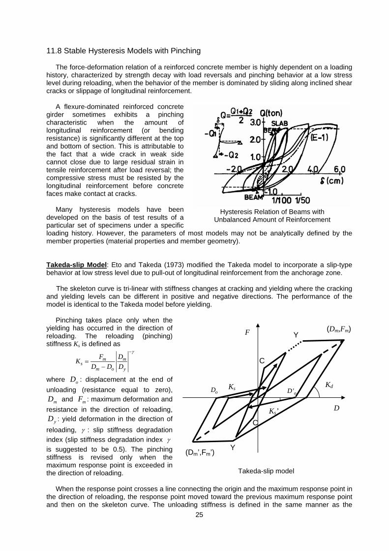
The force-deformation relation of a reinforced concrete member is highly dependent on a loading history, characterized by strength decay with load reversals and pinching behavior at a low stress level during reloading, when the behavior of the member is dominated by sliding along inclined shear cracks or slippage of longitudinal reinforcement.
A flexure-dominated reinforced concrete girder sometimes exhibits a pinching characteristic when the amount of longitudinal reinforcement (or bending resistance) is significantly different at the top and bottom of section. This is attributable to the fact that a wide crack in weak side cannot close due to large residual strain in tensile reinforcement after load reversal; the compressive stress must be resisted by the longitudinal reinforcement before concrete faces make contact at cracks.
Many hysteresis models have been developed on the basis of test results of a particular set of specimens under a specific loading history. However, the parameters of most models may not be analytically defined by the member properties (material properties and member geometry). Takeda-slip Model: Eto and Takeda (1973) modified the Takeda model to incorporate a slip-type behavior at low stress level due to pull-out of longitudinal reinforcement from the anchorage zone.
The skeleton curve is tri-linear with stiffness changes at cracking and yielding where the cracking and yielding levels can be different in positive and negative directions. The performance of the model is identical to the Takeda model before yielding.
Pinching takes place only when the yielding has occurred in the direction of reloading. The reloading (pinching) stiffness Ks is defined as
m ms
m o y
F DKD D D
γ−
=−
where oD : displacement at the end of unloading (resistance equal to zero),
mD and mF : maximum deformation and resistance in the direction of reloading,
yD : yield deformation in the direction of reloading, γ : slip stiffness degradation index (slip stiffness degradation index γ is suggested to be 0.5). The pinching stiffness is revised only when the maximum response point is exceeded in the direction of reloading.
When the response point crosses a line connecting the origin and the maximum response point in the direction of reloading, the response point moved toward the previous maximum response point and then on the skeleton curve. The unloading stiffness is defined in the same manner as the
D
F Y (Dm,Fm)
KdoD
C
C
Y
Ks
Ks’
(Dm’,Fm’)
'oD
Takeda-slip model
Hysteresis Relation of Beams with Unbalanced Amount of Reinforcement
26
Takeda model. The same pinching and unloading stiffness is used during reloading and unloading in an inner
loop.
''c y m
dc y y
F F DKD D D
α−+
=+
where, 'cF and 'cD : resistance and deformation at cracking on the opposite side, yF and yD :
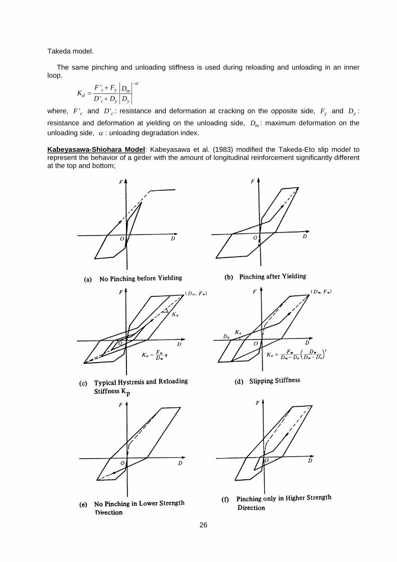
resistance and deformation at yielding on the unloading side, mD : maximum deformation on the unloading side, α : unloading degradation index. Kabeyasawa-Shiohara Model: Kabeyasawa et al. (1983) modified the Takeda-Eto slip model to represent the behavior of a girder with the amount of longitudinal reinforcement significantly different at the top and bottom;
27
(1) the pinching occurs only in one direction where the yield resistance is higher than the other direction,
(2) the pinching occurs only after the initial yielding in the direction of reloading, and (3) the stiffness Ks during slipping is a function of the maximum response point (Dm, Fm) and the
point of load reversal (Do, Fo=0.0) in the resistance-deformation plane.
The reloading (slip) stiffness Ks, after unloading in the direction of the smaller yield resistance, was determined as
γ
om
m
om
ms DD
DDD
FK−−
=
where ( mm FD , ): deformation and resistance at the previous maximum response point, oD : displacement at the end of unloading on the zero-load axis, γ : slip stiffness degradation index. No slip behavior will be generated for γ = 0; the degree of slip behavior increases with γ > 1.0. γ = 1.2 was suggested.
The slip stiffness is used until the response point crosses a line with slope Kp through the previous maximum response point (Dm, Fm); the stiffness is reduced from the slope connecting the origin and the maximum response point by reloading stiffness index η ,
)(m
mp D
FK η=
The values of unloading stiffness degradation index α of Takeda model, slipping stiffness
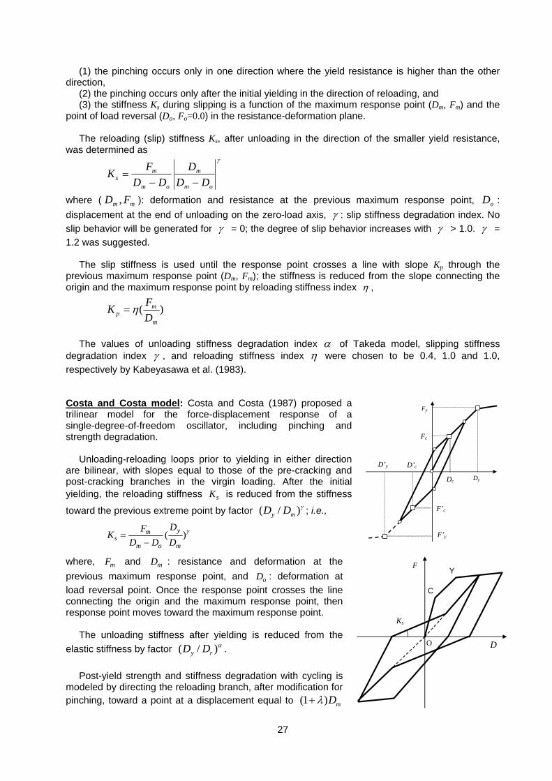
degradation index γ , and reloading stiffness index η were chosen to be 0.4, 1.0 and 1.0, respectively by Kabeyasawa et al. (1983). Costa and Costa model: Costa and Costa (1987) proposed a trilinear model for the force-displacement response of a single-degree-of-freedom oscillator, including pinching and strength degradation.
Unloading-reloading loops prior to yielding in either direction are bilinear, with slopes equal to those of the pre-cracking and post-cracking branches in the virgin loading. After the initial yielding, the reloading stiffness sK is reduced from the stiffness
toward the previous extreme point by factor ( / )y mD D γ ; i.e.,
( )yms
m o m
DFKD D D
γ=−
where, mF and mD : resistance and deformation at the previous maximum response point, and oD : deformation at load reversal point. Once the response point crosses the line connecting the origin and the maximum response point, then response point moves toward the maximum response point.
The unloading stiffness after yielding is reduced from the elastic stiffness by factor ( / )y rD D α .
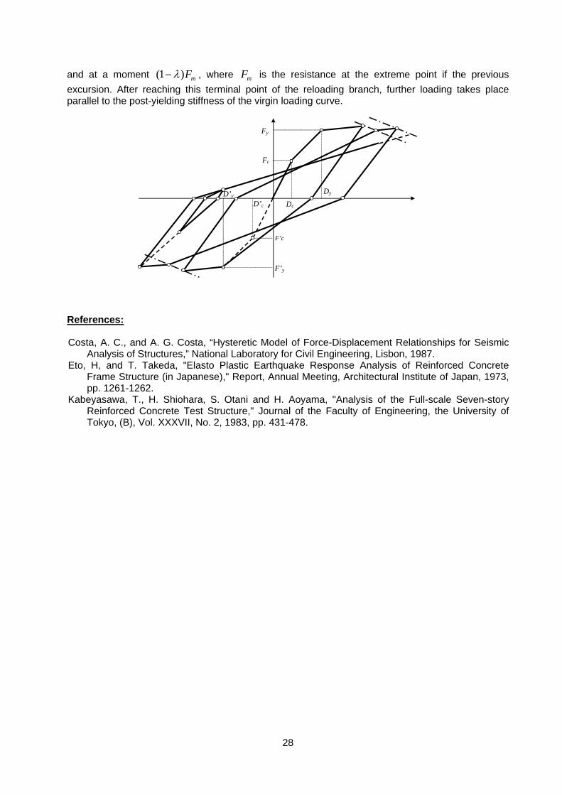
Post-yield strength and stiffness degradation with cycling is modeled by directing the reloading branch, after modification for pinching, toward a point at a displacement equal to (1 ) mDλ+
D
F
C
Y
Ks
O
Dc Dy
Fc
Fy
F’c
F’y
D’c D’y
28
and at a moment (1 ) mFλ− , where mF is the resistance at the extreme point if the previous excursion. After reaching this terminal point of the reloading branch, further loading takes place parallel to the post-yielding stiffness of the virgin loading curve.
References: Costa, A. C., and A. G. Costa, “Hysteretic Model of Force-Displacement Relationships for Seismic
Analysis of Structures,” National Laboratory for Civil Engineering, Lisbon, 1987. Eto, H, and T. Takeda, "Elasto Plastic Earthquake Response Analysis of Reinforced Concrete
Frame Structure (in Japanese)," Report, Annual Meeting, Architectural Institute of Japan, 1973, pp. 1261-1262.
Kabeyasawa, T., H. Shiohara, S. Otani and H. Aoyama, "Analysis of the Full-scale Seven-story Reinforced Concrete Test Structure," Journal of the Faculty of Engineering, the University of Tokyo, (B), Vol. XXXVII, No. 2, 1983, pp. 431-478.
F’c
F’y
D’c
D’y
Dc
Dy
Fc
Fy
29
11.9 Shear-type Hysteresis Models
Reinforced concrete members exhibit progressive loss of strength under reversed cycles of inelastic deformation due to lack of shear capacity of member or bond resistance along longitudinal reinforcement; the monotonic strength of such members cannot be attained.
The response of a reinforced concrete member, exhibiting early strength decay, is difficult to model because such behavior is sensitive to loading history. General features can be summarized as the decay in resistance with cyclic loading and pinching response during reloading followed by hardening.
The undesirable features can be avoided or reduced by following design requirements and
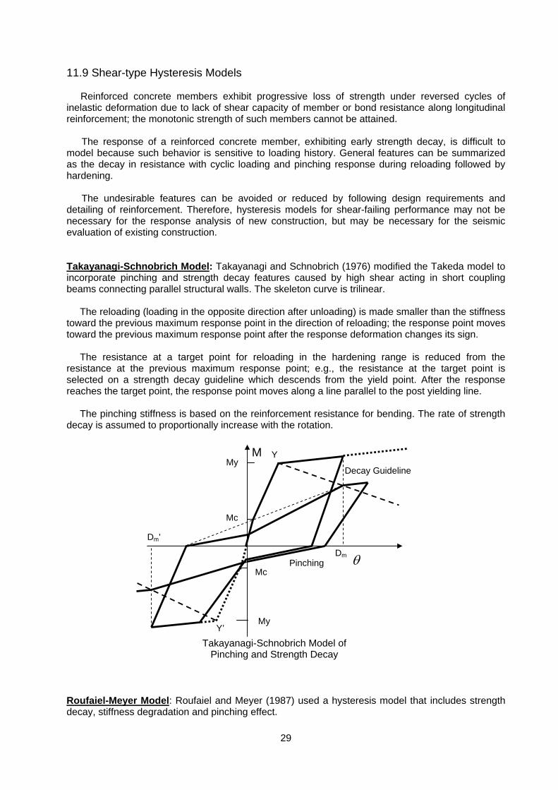
detailing of reinforcement. Therefore, hysteresis models for shear-failing performance may not be necessary for the response analysis of new construction, but may be necessary for the seismic evaluation of existing construction. Takayanagi-Schnobrich Model: Takayanagi and Schnobrich (1976) modified the Takeda model to incorporate pinching and strength decay features caused by high shear acting in short coupling beams connecting parallel structural walls. The skeleton curve is trilinear.
The reloading (loading in the opposite direction after unloading) is made smaller than the stiffness toward the previous maximum response point in the direction of reloading; the response point moves toward the previous maximum response point after the response deformation changes its sign.
The resistance at a target point for reloading in the hardening range is reduced from the resistance at the previous maximum response point; e.g., the resistance at the target point is selected on a strength decay guideline which descends from the yield point. After the response reaches the target point, the response point moves along a line parallel to the post yielding line.
The pinching stiffness is based on the reinforcement resistance for bending. The rate of strength decay is assumed to proportionally increase with the rotation.
Roufaiel-Meyer Model: Roufaiel and Meyer (1987) used a hysteresis model that includes strength decay, stiffness degradation and pinching effect.
Pinching
Decay Guideline
M
Mc
Mc
My
My
θDm
Dm’
Y’
Y
Takayanagi-Schnobrich Model of
Pinching and Strength Decay
30
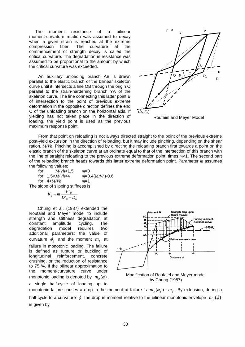
The moment resistance of a bilinear moment-curvature relation was assumed to decay when a given strain is reached at the extreme compression fiber. The curvature at the commencement of strength decay is called the critical curvature. The degradation in resistance was assumed to be proportional to the amount by which the critical curvature was exceeded.
An auxiliary unloading branch AB is drawn parallel to the elastic branch of the bilinear skeleton curve until it intersects a line OB through the origin O parallel to the strain-hardening branch YA of the skeleton curve. The line connecting this latter point B of intersection to the point of previous extreme deformation in the opposite direction defines the end C of the unloading branch on the horizontal axis. If yielding has not taken place in the direction of loading, the yield point is used as the previous maximum response point.
From that point on reloading is not always directed straight to the point of the previous extreme
post-yield excursion in the direction of reloading, but it may include pinching, depending on the shear ration, M/Vh. Pinching is accomplished by directing the reloading branch first towards a point on the elastic branch of the skeleton curve at an ordinate equal to that of the intersection of this branch with the line of straight reloading to the previous extreme deformation point, times m<1. The second part of the reloading branch heads towards this latter extreme deformation point. Parameter m assumes the following values;
for M/Vh<1.5 m=0 for 1.5<M/Vh<4 m=0.4(M/Vh)-0.6 for 4<M/Vh m=1
The slope of slipping stiffness is
''
ms
m o
FK mD D
=−
Chung et al. (1987) extended the
Roufaiel and Meyer model to include strength and stiffness degradation at constant amplitude cycling. The degradation model requires two additional parameters: the value of curvature fφ and the moment fm at failure in monotonic loading. The failure is defined as rupture or buckling of longitudinal reinforcement, concrete crushing, or the reduction of resistance to 75 %. If the bilinear approximation to the moment-curvature curve under monotonic loading is denoted by ( )pm φ , a single half-cycle of loading up to monotonic failure causes a drop in the moment at failure is ( )p f fm mφ − . By extension, during a
half-cycle to a curvature φ the drop in moment relative to the bilinear monotonic envelope ( )pm φ is given by
Modification of Roufaiel and Meyer model by Chung (1987)
Y F A
B
C D
O sK oD
(Dm,Fm)
Roufaiel and Meyer Model
31
32
( ) { ( ) } yp f f
f y
m half cycle at m mφ φ
φ φφ φ⎛ ⎞−
Δ = − ⎜ ⎟⎜ ⎟−⎝ ⎠
Accordingly, a branch of reloading in the direction where the previous maximum curvature is equal to φ , moves toward a point at ( ( ) ,pm mφ φ−Δ ), rather than at ( ( ),pm φ φ ) as in the original Roufaiel and Meyer model.
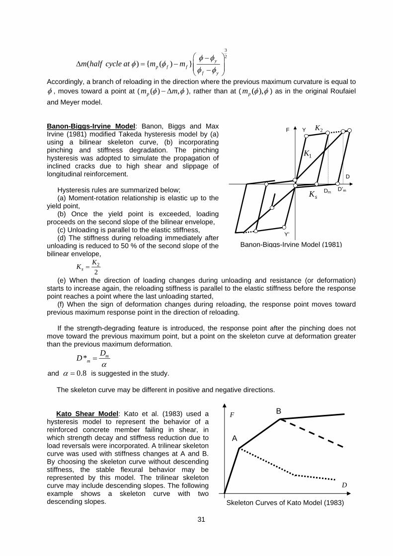
Banon-Biggs-Irvine Model: Banon, Biggs and Max Irvine (1981) modified Takeda hysteresis model by (a) using a bilinear skeleton curve, (b) incorporating pinching and stiffness degradation. The pinching hysteresis was adopted to simulate the propagation of inclined cracks due to high shear and slippage of longitudinal reinforcement.
Hysteresis rules are summarized below; (a) Moment-rotation relationship is elastic up to the
yield point, (b) Once the yield point is exceeded, loading
proceeds on the second slope of the bilinear envelope, (c) Unloading is parallel to the elastic stiffness, (d) The stiffness during reloading immediately after
unloading is reduced to 50 % of the second slope of the bilinear envelope,
2
2sKK =
(e) When the direction of loading changes during unloading and resistance (or deformation) starts to increase again, the reloading stiffness is parallel to the elastic stiffness before the response point reaches a point where the last unloading started,
(f) When the sign of deformation changes during reloading, the response point moves toward previous maximum response point in the direction of reloading.
If the strength-degrading feature is introduced, the response point after the pinching does not
move toward the previous maximum point, but a point on the skeleton curve at deformation greater than the previous maximum deformation.
* mm
DDα
=
and 0.8α = is suggested in the study.
The skeleton curve may be different in positive and negative directions.
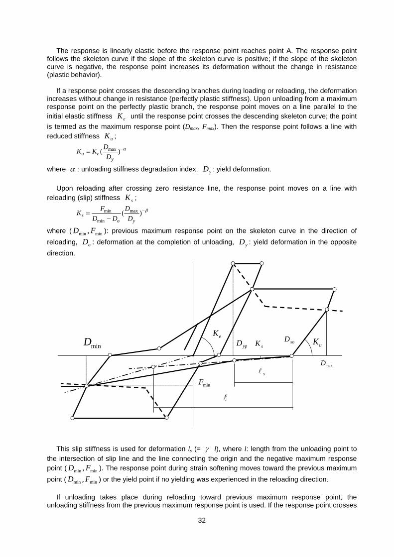
Kato Shear Model: Kato et al. (1983) used a hysteresis model to represent the behavior of a reinforced concrete member failing in shear, in which strength decay and stiffness reduction due to load reversals were incorporated. A trilinear skeleton curve was used with stiffness changes at A and B. By choosing the skeleton curve without descending stiffness, the stable flexural behavior may be represented by this model. The trilinear skeleton curve may include descending slopes. The following example shows a skeleton curve with two descending slopes.
F
D
Y
Y’
Dm D’msK
1K
2K
Banon-Biggs-Irvine Model (1981)
D
F
A
B
Skeleton Curves of Kato Model (1983)
32
The response is linearly elastic before the response point reaches point A. The response point follows the skeleton curve if the slope of the skeleton curve is positive; if the slope of the skeleton curve is negative, the response point increases its deformation without the change in resistance (plastic behavior).
If a response point crosses the descending branches during loading or reloading, the deformation
increases without change in resistance (perfectly plastic stiffness). Upon unloading from a maximum response point on the perfectly plastic branch, the response point moves on a line parallel to the initial elastic stiffness eK until the response point crosses the descending skeleton curve; the point is termed as the maximum response point (Dmax, Fmax). Then the response point follows a line with reduced stiffness uK ;
max( )u ey
DK KD
α−=
where α : unloading stiffness degradation index, yD : yield deformation.
Upon reloading after crossing zero resistance line, the response point moves on a line with reloading (slip) stiffness sK ;
maxmin
min( )s
o y
DFKD D D
β−=−
where ( minmin , FD ): previous maximum response point on the skeleton curve in the direction of reloading, oD : deformation at the completion of unloading, yD : yield deformation in the opposite direction.
This slip stiffness is used for deformation ls (= γ l), where l: length from the unloading point to
the intersection of slip line and the line connecting the origin and the negative maximum response point ( minmin , FD ). The response point during strain softening moves toward the previous maximum point ( minmin , FD ) or the yield point if no yielding was experienced in the reloading direction.
If unloading takes place during reloading toward previous maximum response point, the
unloading stiffness from the previous maximum response point is used. If the response point crosses
s
minF
minD
maxD
xoD ypD
eK
sK uK
33
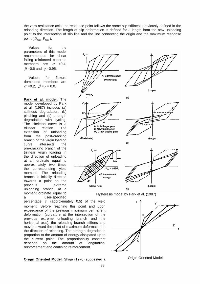
the zero resistance axis, the response point follows the same slip stiffness previously defined in the reloading direction. The length of slip deformation is defined for l: length from the new unloading point to the intersection of slip line and the line connecting the origin and the maximum response point ( max max,D F ).
Values for the
parameters of this model recommended for shear failing reinforced concrete members are α =0.4, β =0.6 and γ =0.95.
Values for flexure dominated members are α =0.2, β =γ = 0.0. Park et al. model: The model developed by Park et al. (1987) includes (a) stiffness degradation, (b) pinching and (c) strength degradation with cycling. The skeleton curve is a trilinear relation. The extension of unloading from the post-cracking branch of the virgin loading curve intersects the pre-cracking branch of the trilinear virgin loading in the direction of unloading at an ordinate equal to approximately two times the corresponding yield moment. The reloading branch is initially directed towards a point on the previous extreme unloading branch, at a moment ordinate equal to a user-specified percentage γ (approximately 0.5) of the yield moment. Before reaching this point and upon exceedance of the previous maximum permanent deformation (curvature at the intersection of the previous extreme unloading branch and the horizontal axis), the reloading branch stiffens and moves toward the point of maximum deformation in the direction of reloading. The strength degrades in proportion to the amount of energy dissipated up to the current point. The proportionality constant depends on the amount of longitudinal reinforcement and confining reinforcement. Origin Oriented Model: Shiga (1976) suggested a
Hysteresis model by Park et al. (1987)
D
F
C
Y
C
Y
Origin-Oriented Model
34
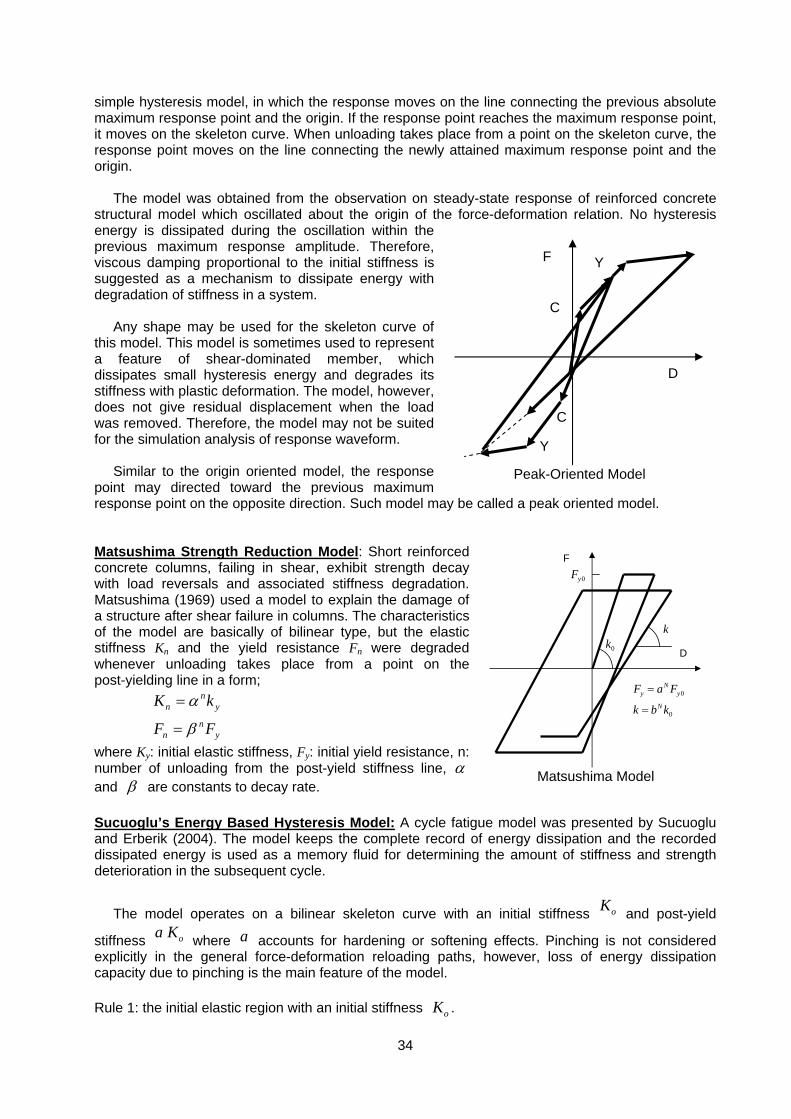
simple hysteresis model, in which the response moves on the line connecting the previous absolute maximum response point and the origin. If the response point reaches the maximum response point, it moves on the skeleton curve. When unloading takes place from a point on the skeleton curve, the response point moves on the line connecting the newly attained maximum response point and the origin.
The model was obtained from the observation on steady-state response of reinforced concrete structural model which oscillated about the origin of the force-deformation relation. No hysteresis energy is dissipated during the oscillation within the previous maximum response amplitude. Therefore, viscous damping proportional to the initial stiffness is suggested as a mechanism to dissipate energy with degradation of stiffness in a system.
Any shape may be used for the skeleton curve of this model. This model is sometimes used to represent a feature of shear-dominated member, which dissipates small hysteresis energy and degrades its stiffness with plastic deformation. The model, however, does not give residual displacement when the load was removed. Therefore, the model may not be suited for the simulation analysis of response waveform.
Similar to the origin oriented model, the response
point may directed toward the previous maximum response point on the opposite direction. Such model may be called a peak oriented model. Matsushima Strength Reduction Model: Short reinforced concrete columns, failing in shear, exhibit strength decay with load reversals and associated stiffness degradation. Matsushima (1969) used a model to explain the damage of a structure after shear failure in columns. The characteristics of the model are basically of bilinear type, but the elastic stiffness Kn and the yield resistance Fn were degraded whenever unloading takes place from a point on the post-yielding line in a form;
y
nn
yn
n
FF
kK
β
α
=
=
where Ky: initial elastic stiffness, Fy: initial yield resistance, n: number of unloading from the post-yield stiffness line, α and β are constants to decay rate. Sucuoglu’s Energy Based Hysteresis Model: A cycle fatigue model was presented by Sucuoglu and Erberik (2004). The model keeps the complete record of energy dissipation and the recorded dissipated energy is used as a memory fluid for determining the amount of stiffness and strength deterioration in the subsequent cycle.
The model operates on a bilinear skeleton curve with an initial stiffness oK and post-yield
stiffness oa K where a accounts for hardening or softening effects. Pinching is not considered explicitly in the general force-deformation reloading paths, however, loss of energy dissipation capacity due to pinching is the main feature of the model. Rule 1: the initial elastic region with an initial stiffness oK .
D
F
C
Y
C
Y
Peak-Oriented Model
F
D0k
0
0
Ny y
N
F a F
k b k
=
=
0yF
k
Matsushima Model
35
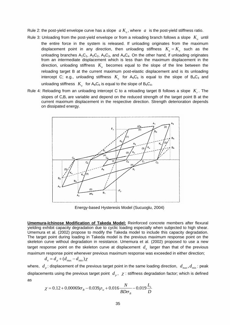
Rule 2: the post-yield envelope curve has a slope oa K , where a is the post-yield stiffness ratio.
Rule 3: Unloading from the post-yield envelope or from a reloading branch follows a slope oK until the entire force in the system is released. If unloading originates from the maximum displacement point in any direction, then unloading stiffness u oK K= such as the unloading branches A1C1, A2C2, A3C3, and A4C4. On the other hand, if unloading originates from an intermediate displacement which is less than the maximum displacement in the direction, unloading stiffness uK becomes equal to the slope of the line between the reloading target B at the current maximum post-elastic displacement and is its unloading intercept C; e.g., unloading stiffness uK for A5C5 is equal to the slope of B4C3 and
unloading stiffness uK for A6C6 is equal to the slope of B5C4.
Rule 4: Reloading from an unloading intercept C to a reloading target B follows a slope rK . The slopes of CiBi are variable and depend on the reduced strength of the target point B at the current maximum displacement in the respective direction. Strength deterioration depends on dissipated energy.
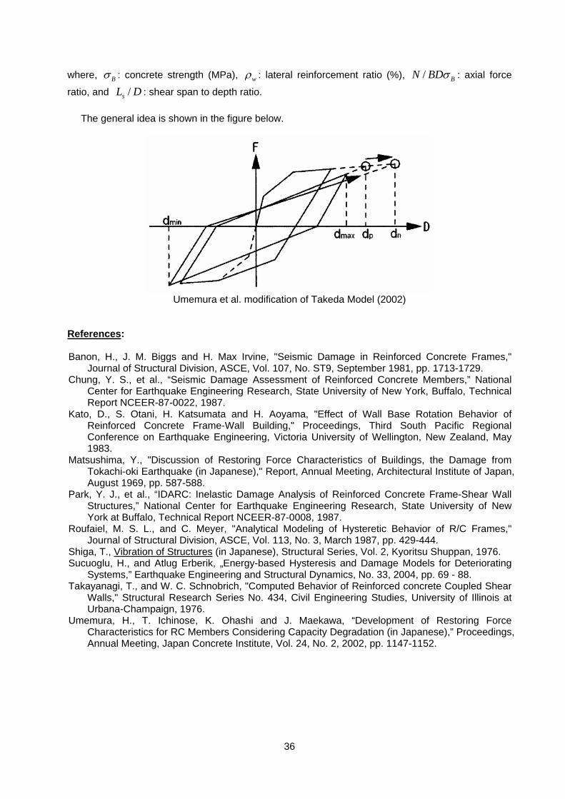
Umemura-Ichinose Modification of Takeda Model: Reinforced concrete members after flexural yielding exhibit capacity degradation due to cyclic loading especially when subjected to high shear. Umemura et al. (2002) propose to modify the Takeda model to include this capacity degradation. The target point during loading in Takeda model is the previous maximum response point on the skeleton curve without degradation in resistance. Umemura et al. (2002) proposed to use a new target response point on the skeleton curve at displacement nd larger than that of the previous maximum response point whenever previous maximum response was exceeded in either direction; n max min( )pd d d d χ= + −
where, pd : displacement of the previous target point in the same loading direction, max min,d d : peak
displacements using the previous target point pd , χ : stiffness degradation factor; which is defined as
0.12 0.00069 0.039 0.016 0.019 sB w
B
LNBD D
χ σ ρσ
= + − + −
Energy-based Hysteresis Model (Sucuoglu, 2004)
36
where, Bσ : concrete strength (MPa), wρ : lateral reinforcement ratio (%), / BN BDσ : axial force
ratio, and /sL D : shear span to depth ratio.
The general idea is shown in the figure below.
Umemura et al. modification of Takeda Model (2002)
References: Banon, H., J. M. Biggs and H. Max Irvine, "Seismic Damage in Reinforced Concrete Frames,"
Journal of Structural Division, ASCE, Vol. 107, No. ST9, September 1981, pp. 1713-1729. Chung, Y. S., et al., “Seismic Damage Assessment of Reinforced Concrete Members,” National
Center for Earthquake Engineering Research, State University of New York, Buffalo, Technical Report NCEER-87-0022, 1987.
Kato, D., S. Otani, H. Katsumata and H. Aoyama, "Effect of Wall Base Rotation Behavior of Reinforced Concrete Frame-Wall Building," Proceedings, Third South Pacific Regional Conference on Earthquake Engineering, Victoria University of Wellington, New Zealand, May 1983.
Matsushima, Y., "Discussion of Restoring Force Characteristics of Buildings, the Damage from Tokachi-oki Earthquake (in Japanese)," Report, Annual Meeting, Architectural Institute of Japan, August 1969, pp. 587-588.
Park, Y. J., et al., “IDARC: Inelastic Damage Analysis of Reinforced Concrete Frame-Shear Wall Structures,” National Center for Earthquake Engineering Research, State University of New York at Buffalo, Technical Report NCEER-87-0008, 1987.
Roufaiel, M. S. L., and C. Meyer, "Analytical Modeling of Hysteretic Behavior of R/C Frames," Journal of Structural Division, ASCE, Vol. 113, No. 3, March 1987, pp. 429-444.
Shiga, T., Vibration of Structures (in Japanese), Structural Series, Vol. 2, Kyoritsu Shuppan, 1976. Sucuoglu, H., and Atlug Erberik, „Energy-based Hysteresis and Damage Models for Deteriorating
Systems,” Earthquake Engineering and Structural Dynamics, No. 33, 2004, pp. 69 - 88. Takayanagi, T., and W. C. Schnobrich, "Computed Behavior of Reinforced concrete Coupled Shear
Walls," Structural Research Series No. 434, Civil Engineering Studies, University of Illinois at Urbana-Champaign, 1976.
Umemura, H., T. Ichinose, K. Ohashi and J. Maekawa, “Development of Restoring Force Characteristics for RC Members Considering Capacity Degradation (in Japanese),” Proceedings, Annual Meeting, Japan Concrete Institute, Vol. 24, No. 2, 2002, pp. 1147-1152.
37
11.10 Ibara-Medina-Krawinkler Model
The cyclic hysteretic response of a structural member tested in the laboratory indicates that (1) strength deteriorates with the number and amplitude of cycles, even if the displacement associated with the strength has not been reached, (2) Strength deterioration occurs after reaching the maximum resistance, (3) Unloading stiffness may also deteriorates, and (4) The reloading stiffness may deteriorates at an accelerated rate (Ibara, Medina and Krawinkler, 2005).
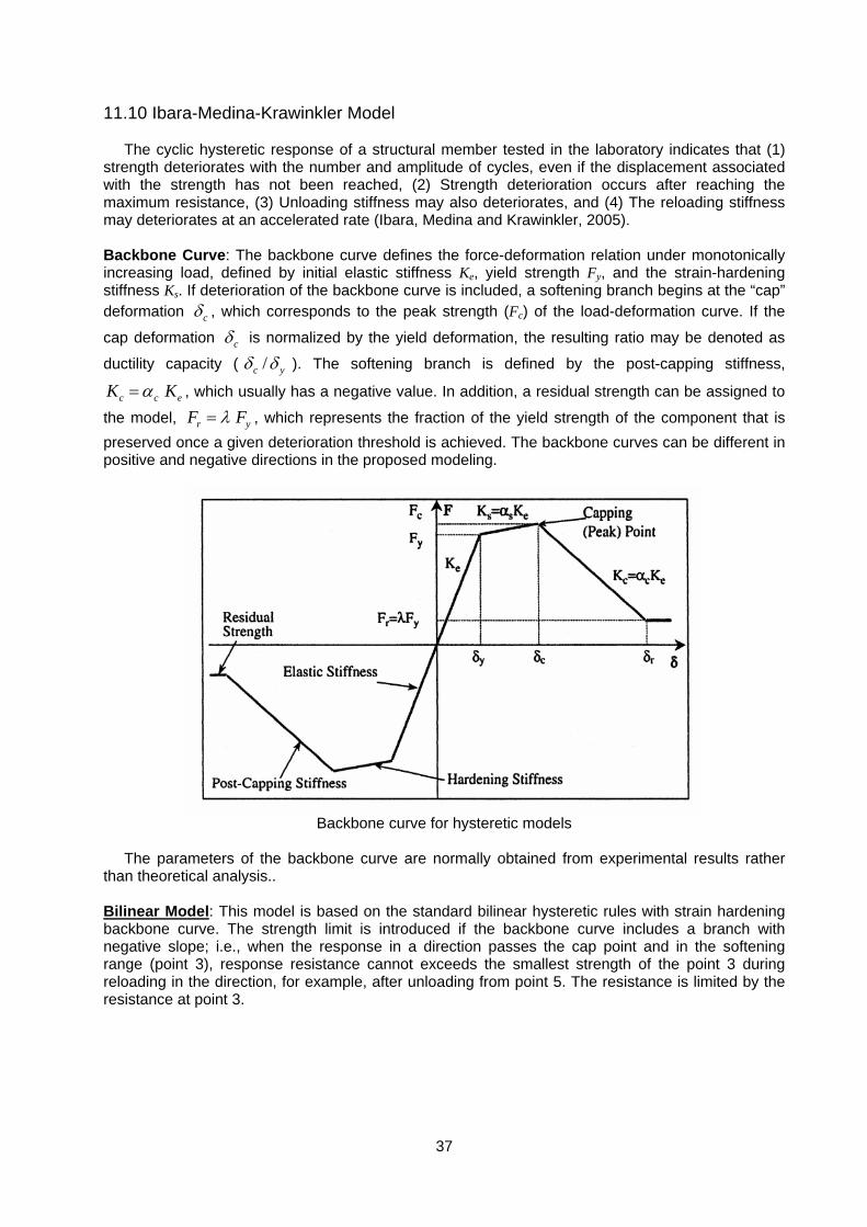
Backbone Curve: The backbone curve defines the force-deformation relation under monotonically increasing load, defined by initial elastic stiffness Ke, yield strength Fy, and the strain-hardening stiffness Ks. If deterioration of the backbone curve is included, a softening branch begins at the “cap” deformation cδ , which corresponds to the peak strength (Fc) of the load-deformation curve. If the
cap deformation cδ is normalized by the yield deformation, the resulting ratio may be denoted as
ductility capacity ( /c yδ δ ). The softening branch is defined by the post-capping stiffness,
c c eK Kα= , which usually has a negative value. In addition, a residual strength can be assigned to
the model, r yF Fλ= , which represents the fraction of the yield strength of the component that is preserved once a given deterioration threshold is achieved. The backbone curves can be different in positive and negative directions in the proposed modeling.
Backbone curve for hysteretic models
The parameters of the backbone curve are normally obtained from experimental results rather
than theoretical analysis..
Bilinear Model: This model is based on the standard bilinear hysteretic rules with strain hardening backbone curve. The strength limit is introduced if the backbone curve includes a branch with negative slope; i.e., when the response in a direction passes the cap point and in the softening range (point 3), response resistance cannot exceeds the smallest strength of the point 3 during reloading in the direction, for example, after unloading from point 5. The resistance is limited by the resistance at point 3.
38
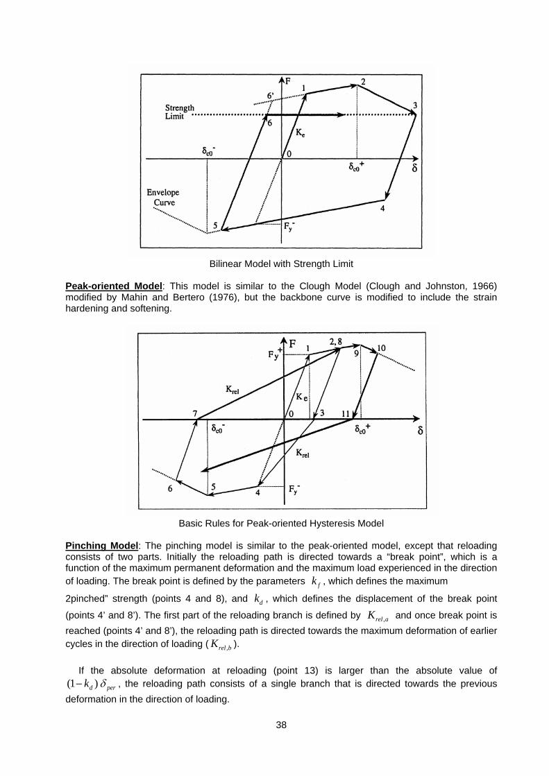
Bilinear Model with Strength Limit
Peak-oriented Model: This model is similar to the Clough Model (Clough and Johnston, 1966) modified by Mahin and Bertero (1976), but the backbone curve is modified to include the strain hardening and softening.
Basic Rules for Peak-oriented Hysteresis Model
Pinching Model: The pinching model is similar to the peak-oriented model, except that reloading consists of two parts. Initially the reloading path is directed towards a “break point”, which is a function of the maximum permanent deformation and the maximum load experienced in the direction of loading. The break point is defined by the parameters fk , which defines the maximum
2pinched” strength (points 4 and 8), and dk , which defines the displacement of the break point
(points 4’ and 8’). The first part of the reloading branch is defined by ,rel aK and once break point is reached (points 4’ and 8’), the reloading path is directed towards the maximum deformation of earlier cycles in the direction of loading ( ,rel bK ).
If the absolute deformation at reloading (point 13) is larger than the absolute value of (1 )d perk δ− , the reloading path consists of a single branch that is directed towards the previous deformation in the direction of loading.
39
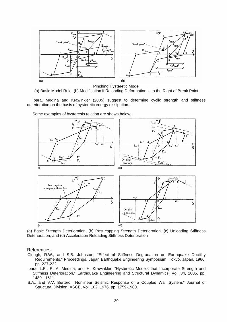
Pinching Hysteretic Model
(a) Basic Model Rule, (b) Modification if Reloading Deformation is to the Right of Break Point
Ibara, Medina and Krawinkler (2005) suggest to determine cyclic strength and stiffness deterioration on the basis of hysteretic energy dissipation.
Some examples of hysteresis relation are shown below;
(a) Basic Strength Deterioration, (b) Post-capping Strength Deterioration, (c) Unloading Stiffness Deterioration, and (d) Acceleration Reloading Stiffness Deterioration
References: Clough, R.W., and S.B. Johnston, “Effect of Stiffness Degradation on Earthquake Ductility
Requirements,” Proceedings, Japan Earthquake Engineering Symposium, Tokyo, Japan, 1966, pp. 227-232.
Ibara, L.F., R. A. Medina, and H. Krawinkler, “Hysteretic Models that Incorporate Strength and Stiffness Deterioration,” Earthquake Engineering and Structural Dynamics, Vol. 34, 2005, pp. 1489 - 1511.
S.A., and V.V. Bertero, “Nonlinear Seismic Response of a Coupled Wall System,” Journal of Structural Division, ASCE, Vol. 102, 1976, pp. 1759-1980.
40
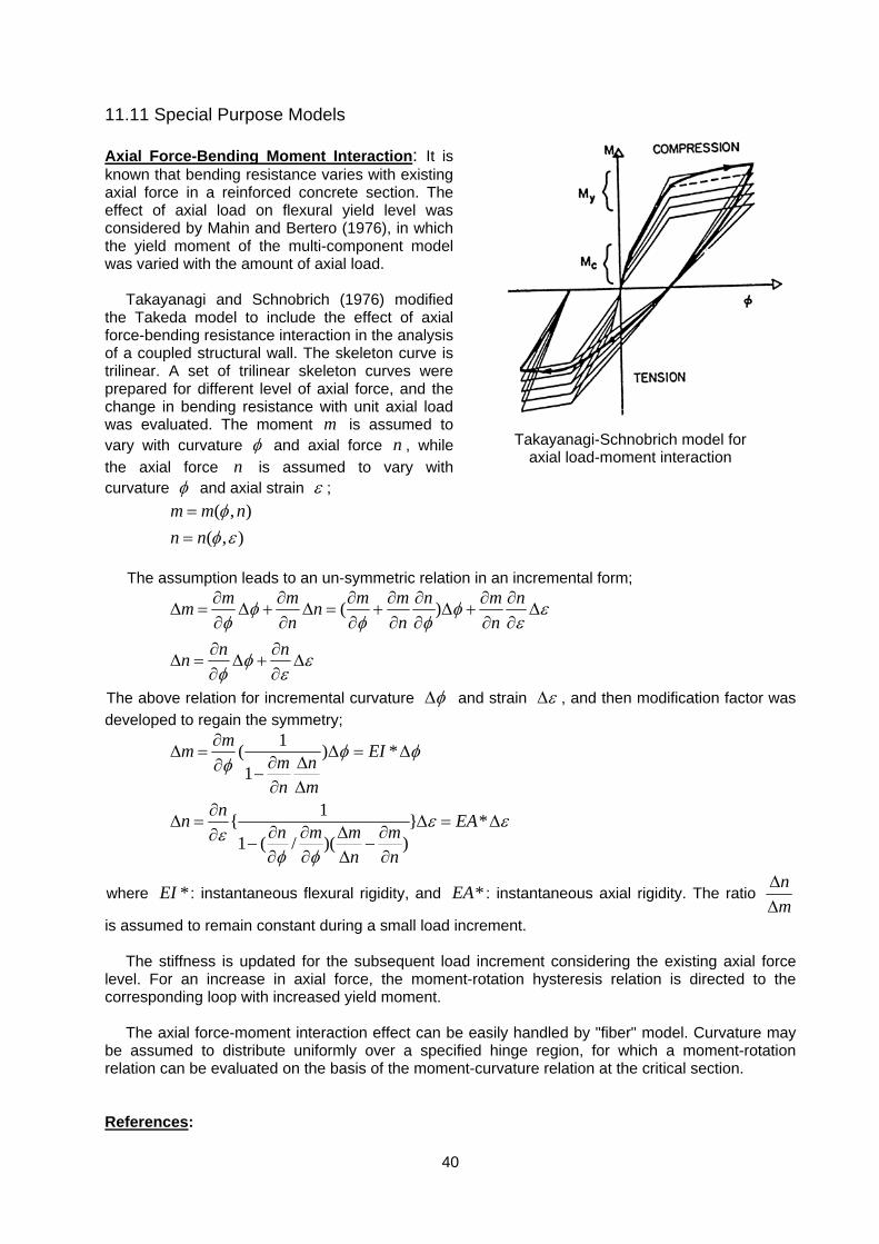
11.11 Special Purpose Models Axial Force-Bending Moment Interaction: It is known that bending resistance varies with existing axial force in a reinforced concrete section. The effect of axial load on flexural yield level was considered by Mahin and Bertero (1976), in which the yield moment of the multi-component model was varied with the amount of axial load.
Takayanagi and Schnobrich (1976) modified the Takeda model to include the effect of axial force-bending resistance interaction in the analysis of a coupled structural wall. The skeleton curve is trilinear. A set of trilinear skeleton curves were prepared for different level of axial force, and the change in bending resistance with unit axial load was evaluated. The moment m is assumed to vary with curvature φ and axial force n , while the axial force n is assumed to vary with curvature φ and axial strain ε ;
( , )
( , )m m nn n
φφ ε
==
The assumption leads to an un-symmetric relation in an incremental form;
( )m m m m n m nm nn n n
n nn
φ φ εφ φ φ ε
φ εφ ε
∂ ∂ ∂ ∂ ∂ ∂ ∂Δ = Δ + Δ = + Δ + Δ
∂ ∂ ∂ ∂ ∂ ∂ ∂∂ ∂
Δ = Δ + Δ∂ ∂
The above relation for incremental curvature φΔ and strain εΔ , and then modification factor was developed to regain the symmetry;
1( ) *1
1{ } *1 ( / )( )
mm EIm nn m
nn EAn m m mn n
φ φφ
ε εε
φ φ
∂Δ = Δ = Δ
∂ Δ∂ −∂ Δ
∂Δ = Δ = Δ
∂ ∂ Δ ∂∂ − −∂ ∂ Δ ∂
where *EI : instantaneous flexural rigidity, and *EA : instantaneous axial rigidity. The ratio nmΔΔ
is assumed to remain constant during a small load increment. The stiffness is updated for the subsequent load increment considering the existing axial force
level. For an increase in axial force, the moment-rotation hysteresis relation is directed to the corresponding loop with increased yield moment.
The axial force-moment interaction effect can be easily handled by "fiber" model. Curvature may be assumed to distribute uniformly over a specified hinge region, for which a moment-rotation relation can be evaluated on the basis of the moment-curvature relation at the critical section. References:
Takayanagi-Schnobrich model for axial load-moment interaction
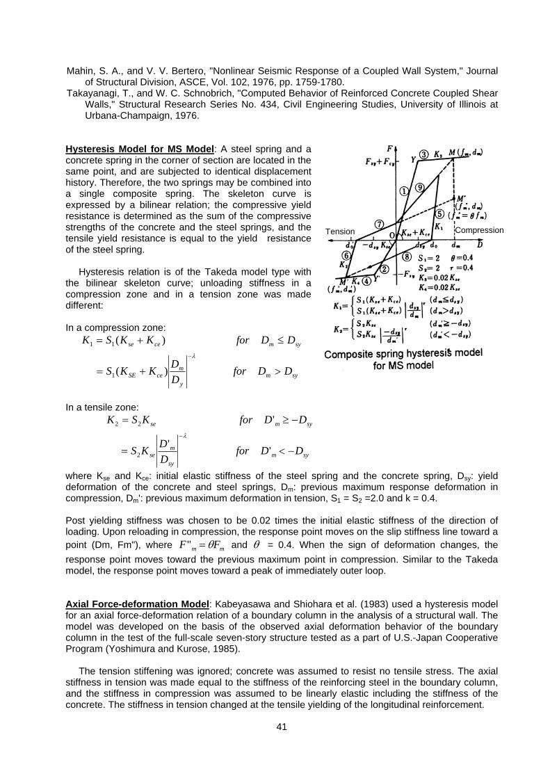
41
Mahin, S. A., and V. V. Bertero, "Nonlinear Seismic Response of a Coupled Wall System," Journal of Structural Division, ASCE, Vol. 102, 1976, pp. 1759-1780.
Takayanagi, T., and W. C. Schnobrich, "Computed Behavior of Reinforced Concrete Coupled Shear Walls," Structural Research Series No. 434, Civil Engineering Studies, University of Illinois at Urbana-Champaign, 1976.
Hysteresis Model for MS Model: A steel spring and a concrete spring in the corner of section are located in the same point, and are subjected to identical displacement history. Therefore, the two springs may be combined into a single composite spring. The skeleton curve is expressed by a bilinear relation; the compressive yield resistance is determined as the sum of the compressive strengths of the concrete and the steel springs, and the tensile yield resistance is equal to the yield resistance of the steel spring.
Hysteresis relation is of the Takeda model type with the bilinear skeleton curve; unloading stiffness in a compression zone and in a tension zone was made different: In a compression zone:
sym
y
mceSE
symcese
DDforDDKKS
DDforKKSK
>+=
≤+=−λ
)(
)(
1
11
In a tensile zone:
sym
sy
mse
symse
DDforDDKS
DDforKSK
−<=
−≥=−
''
'
2
22
λ
where Kse and Kce: initial elastic stiffness of the steel spring and the concrete spring, Dsy: yield deformation of the concrete and steel springs, Dm: previous maximum response deformation in compression, Dm': previous maximum deformation in tension, S1 = S2 =2.0 and k = 0.4. Post yielding stiffness was chosen to be 0.02 times the initial elastic stiffness of the direction of loading. Upon reloading in compression, the response point moves on the slip stiffness line toward a point (Dm, Fm"), where mm FF θ=" and θ = 0.4. When the sign of deformation changes, the response point moves toward the previous maximum point in compression. Similar to the Takeda model, the response point moves toward a peak of immediately outer loop. Axial Force-deformation Model: Kabeyasawa and Shiohara et al. (1983) used a hysteresis model for an axial force-deformation relation of a boundary column in the analysis of a structural wall. The model was developed on the basis of the observed axial deformation behavior of the boundary column in the test of the full-scale seven-story structure tested as a part of U.S.-Japan Cooperative Program (Yoshimura and Kurose, 1985).
The tension stiffening was ignored; concrete was assumed to resist no tensile stress. The axial stiffness in tension was made equal to the stiffness of the reinforcing steel in the boundary column, and the stiffness in compression was assumed to be linearly elastic including the stiffness of the concrete. The stiffness in tension changed at the tensile yielding of the longitudinal reinforcement.
Composite spring hysteresis model for MS model
Tension Compression
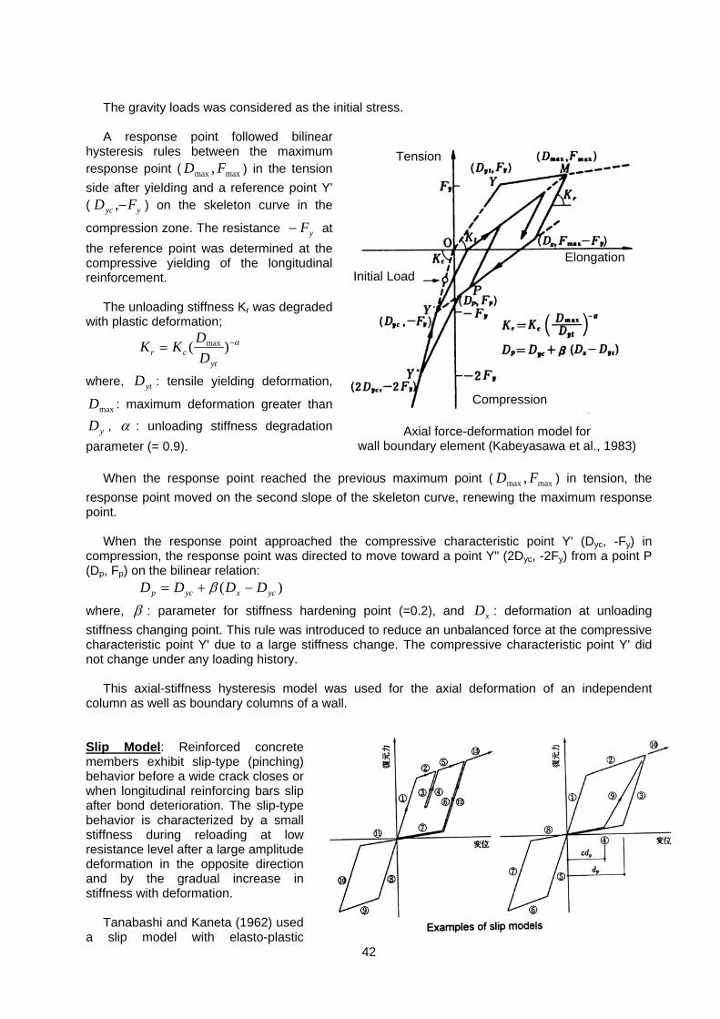
42
The gravity loads was considered as the initial stress.
A response point followed bilinear
hysteresis rules between the maximum response point ( maxmax , FD ) in the tension side after yielding and a reference point Y' ( yyc FD −, ) on the skeleton curve in the
compression zone. The resistance yF− at the reference point was determined at the compressive yielding of the longitudinal reinforcement.
The unloading stiffness Kr was degraded with plastic deformation;
α−= )( max
ytcr D
DKK
where, ytD : tensile yielding deformation,
maxD : maximum deformation greater than
yD , α : unloading stiffness degradation parameter (= 0.9).
When the response point reached the previous maximum point ( maxmax , FD ) in tension, the response point moved on the second slope of the skeleton curve, renewing the maximum response point.
When the response point approached the compressive characteristic point Y' (Dyc, -Fy) in compression, the response point was directed to move toward a point Y" (2Dyc, -2Fy) from a point P (Dp, Fp) on the bilinear relation: )( ycxycp DDDD −+= β
where, β : parameter for stiffness hardening point (=0.2), and xD : deformation at unloading stiffness changing point. This rule was introduced to reduce an unbalanced force at the compressive characteristic point Y' due to a large stiffness change. The compressive characteristic point Y' did not change under any loading history.
This axial-stiffness hysteresis model was used for the axial deformation of an independent column as well as boundary columns of a wall. Slip Model: Reinforced concrete members exhibit slip-type (pinching) behavior before a wide crack closes or when longitudinal reinforcing bars slip after bond deterioration. The slip-type behavior is characterized by a small stiffness during reloading at low resistance level after a large amplitude deformation in the opposite direction and by the gradual increase in stiffness with deformation.
Tanabashi and Kaneta (1962) used a slip model with elasto-plastic
Axial force-deformation model for wall boundary element (Kabeyasawa et al., 1983)
Tension
Initial LoadElongation
Compression
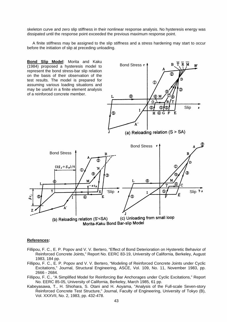
43
skeleton curve and zero slip stiffness in their nonlinear response analysis. No hysteresis energy was dissipated until the response point exceeded the previous maximum response point.
A finite stiffness may be assigned to the slip stiffness and a stress hardening may start to occur before the initiation of slip at preceding unloading. Bond Slip Model: Morita and Kaku (1984) proposed a hysteresis model to represent the bond stress-bar slip relation on the basis of their observation of the test results. The model is prepared for assuming various loading situations and may be useful in a finite element analysis of a reinforced concrete member.
References: Fillipou, F. C., E. P. Popov and V. V. Bertero, “Effect of Bond Deterioration on Hysteretic Behavior of
Reinforced Concrete Joints,” Report No. EERC 83-19, University of California, Berkeley, August 1983, 184 pp.
Fillipou, F. C., E. P. Popov and V. V. Bertero, “Modeling of Reinforced Concrete Joints under Cyclic Excitations,” Journal, Structural Engineering, ASCE, Vol. 109, No. 11, November 1983, pp. 2666 - 2684.
Fillipou, F. C., “A Simplified Model for Reinforcing Bar Anchorages under Cyclic Excitations,” Report No. EERC 85-05, University of California, Berkeley, March 1985, 61 pp.
Kabeyasawa, T., H. Shiohara, S. Otani and H. Aoyama, "Analysis of the Full-scale Seven-story Reinforced Concrete Test Structure," Journal, Faculty of Engineering, University of Tokyo (B), Vol. XXXVII, No. 2, 1983, pp. 432-478.
(a) Reloading relation (S > SA)
Bond Stress
Bond Stress
Slip Slip
Bond Stress
Slip

44
Li, K.-N., S. Otani and H. Aoyama, "Study on the Elastic-plastic Behavior of Reinforced Concrete Columns subjected to Bi-directional Horizontal Earthquake Forces and Varying Axial Load (in Japanese)," Report, Aoyama Laboratory, Department of Architecture, Faculty of Engineering, University of Tokyo, March 1990.
Morita, S., and T. Kaku, "Slippage of Reinforcement in Beam-column Joint of Reinforced Concrete Frames," Proceedings, Eighth World Conference on Earthquake Engineering, San Francisco, U. S. A., Vol. 6, 1984, pp. 477-484.
Tanabashi, R., and K. Kaneta, "On the Relation between the Restoring Force Characteristics of Structures and the Pattern of Earthquake Ground Motion," Proceedings, Japan National Conference on Earthquake Engineering, November 1962, pp. 57-62.
Yoshimura, M., and Y. Kurose, "Inelastic Behavior of the Building," ACI SP-84, Earthquake Effects on Reinforced Concrete Structures, U.S.-Japan Research, American Concrete Institute, Detroit, 1985, pp. 163-202.
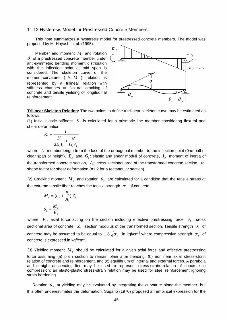
45
11.12 Hysteresis Model for Prestressed Concrete Members
This note summarizes a hysteresis model for prestressed concrete members. The model was proposed by M. Hayashi et al. (1995).
Member end moment M and rotation θ of a prestressed concrete member under anti-symmetric bending moment distribution with the inflection point at mid span is considered. The skeleton curve of the moment-curvature ( , Mθ ) relation is represented by a trilinear relation with stiffness changes at flexural cracking of concrete and tensile yielding of longitudinal reinforcement.
Trilinear Skeleton Relation: The two points to define a trilinear skeleton curve may be estimated as follows. (1) Initial elastic stiffness 1K is calculated for a prismatic line member considering flexural and shear deformation:
1 2
3 c c c c
LKLE I G A
κ=
+
where L : member length from the face of the orthogonal member to the inflection point (0ne-half of clear span or height), cE and cG : elastic and shear moduli of concrete, eI : moment of inertia of
the transformed concrete section, cA : cross sectional area of the transformed concrete section, κ : shape factor for shear deformation (=1.2 for a rectangular section). (2) Cracking moment cM and rotation cθ are calculated for a condition that the tensile stress at
the extreme tensile fiber reaches the tensile strength tσ of concrete:
1
( )ec t e
c
cc
PM ZA
MK
σ
θ
= +
=
where, eP : axial force acting on the section including effective prestressing force, cA : cross
sectional area of concrete, eZ : section modulus of the transformed section. Tensile strength tσ of
concrete may be assumed to be equal to 1.8 Bσ in kgf/cm2 where compressive strength Bσ of concrete is expressed in kgf/cm2. (3) Yielding moment yM should be calculated for a given axial force and effective prestressing force assuming (a) plain section to remain plain after bending, (b) nonlinear axial stress-strain relation of concrete and reinforcement, and (c) equilibrium of internal and external forces. A parabola and straight descending line may be used to represent stress-strain relation of concrete in compression; an elasto-plastic stress-strain relation may be used for steel reinforcement ignoring strain hardening.
Rotation yθ at yielding may be evaluated by integrating the curvature along the member, but this often underestimates the deformation. Sugano (1970) proposed an empirical expression for the
Am
B Am m=
δ
AθB Aθ θ=
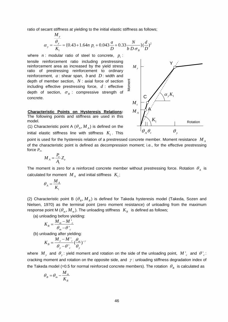
46
ratio of secant stiffness at yielding to the initial elastic stiffness as follows;
2
1
{0.43 1.64 0.043 0.33 }( )
y
yy t
B
Ma N dn p
K D b D Dθ
ασ
= = + + +
where n : modular ratio of steel to concrete, tp : tensile reinforcement ratio including prestressing reinforcement area as increased by the yield stress ratio of prestressing reinforcement to ordinary reinforcement, a : shear span, b and D : width and depth of member section, N : axial force of section including effective prestressing force, d : effective depth of section, Bσ : compressive strength of concrete. Characteristic Points on Hysteresis Relations: The following points and stiffness are used in this model. (1) Characteristic point A ( ,A AMθ ) is defined on the initial elastic stiffness line with stiffness 1K . This point is used for the hysteresis relation of a prestressed concrete member. Moment resistance AM of the characteristic point is defined as decompression moment; i.e., for the effective prestressing force Pe,
eA e
c
PM ZA
=
The moment is zero for a reinforced concrete member without prestressing force. Rotation Aθ is calculated for moment AM and initial stiffness 1K ;
1
AA
MK
θ =
(2) Characteristic point B ( ,B BMθ ) is defined for Takeda hysteresis model (Takeda, Sozen and Nielsen, 1970) as the terminal point (zero moment resistance) of unloading from the maximum response point M ( ,m mMθ ). The unloading stiffness BK is defined as follows;
(a) unloading before yielding:
'
'm c
Bm c
M MKθ θ
−=
−
(b) unloading after yielding:
'
( )'
y c mB
y c y
M MK γθ
θ θ θ−−
=−
where yM and yθ : yield moment and rotation on the side of the unloading point, 'cM and 'cθ : cracking moment and rotation on the opposite side, and γ : unloading stiffness degradation index of the Takeda model (=0.5 for normal reinforced concrete members). The rotation Bθ is calculated as
mB m
B
MK
θ θ= −
C
Y
yθ cθ
cM
yM
Rotation
Mom
ent
1K
1y Kα
A
Aθ
AM
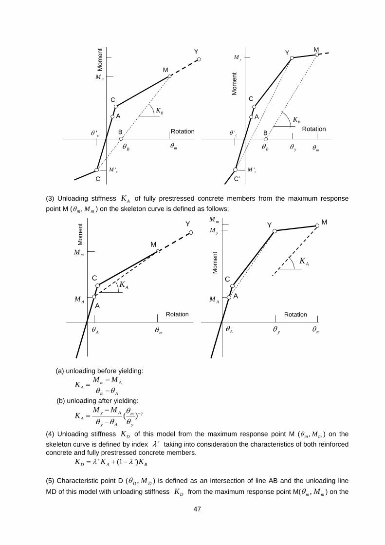
47
C
Y
Rotation
Mom
ent
A
C’ 'cM
'cθ
C
Y
yθ
yM
Rotation
Mom
ent
A
C’'cM
'cθ
MmM
mθ
B
Bθ
BK
B
BK
mθBθ
M
(3) Unloading stiffness AK of fully prestressed concrete members from the maximum response point M ( ,m mMθ ) on the skeleton curve is defined as follows;
C
Y
Rotation
Mom
ent
A
Aθ
AM
M mM
AK C
Y
yθ
yM
Rotation
Mom
ent
A
Aθ
AM
MmM
mθ
AK
mθ
(a) unloading before yielding:
m AA
m A
M MKθ θ
−=
−
(b) unloading after yielding:
( )y A mA
y A y
M MK γθ
θ θ θ−−
=−
(4) Unloading stiffness DK of this model from the maximum response point M ( ,m mMθ ) on the skeleton curve is defined by index 'λ taking into consideration the characteristics of both reinforced concrete and fully prestressed concrete members. ' (1 ')D A BK K Kλ λ= + − (5) Characteristic point D ( ,D DMθ ) is defined as an intersection of line AB and the unloading line MD of this model with unloading stiffness DK from the maximum response point M( ,m mMθ ) on the
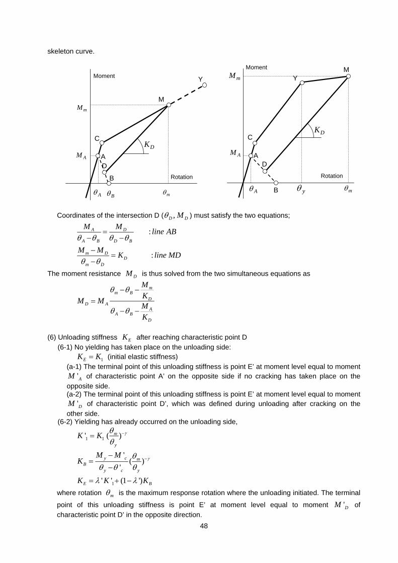
48
skeleton curve.
Coordinates of the intersection D ( ,D DMθ ) must satisfy the two equations;
:
:
A D
A B D B
m DD
m D
M M line AB
M M K line MD
θ θ θ θ
θ θ
=− −−
=−
The moment resistance DM is thus solved from the two simultaneous equations as
mm B
DD A
AA B
D
MKM M MK
θ θ
θ θ
− −=
− −
(6) Unloading stiffness EK after reaching characteristic point D
(6-1) No yielding has taken place on the unloading side: 1EK K= (initial elastic stiffness)
(a-1) The terminal point of this unloading stiffness is point E’ at moment level equal to moment 'AM of characteristic point A’ on the opposite side if no cracking has taken place on the
opposite side. (a-2) The terminal point of this unloading stiffness is point E’ at moment level equal to moment
'DM of characteristic point D’, which was defined during unloading after cracking on the other side.
(6-2) Yielding has already occurred on the unloading side,
1 1
1
' ( )
'( )
'
' ' (1 ')
m
y
y c mB
y c y
E B
K K
M MK
K K K
γ
γ
θθ
θθ θ θ
λ λ
−
−
=
−=
−
= + −
where rotation mθ is the maximum response rotation where the unloading initiated. The terminal
point of this unloading stiffness is point E’ at moment level equal to moment 'DM of characteristic point D’ in the opposite direction.
DK
Rotation
Moment Y
M
C
A D
B
mM
AM
mθBθ Aθ
Rotation
Moment
C
Y M
DK
AD
B
mM
AM
Aθ yθ mθ
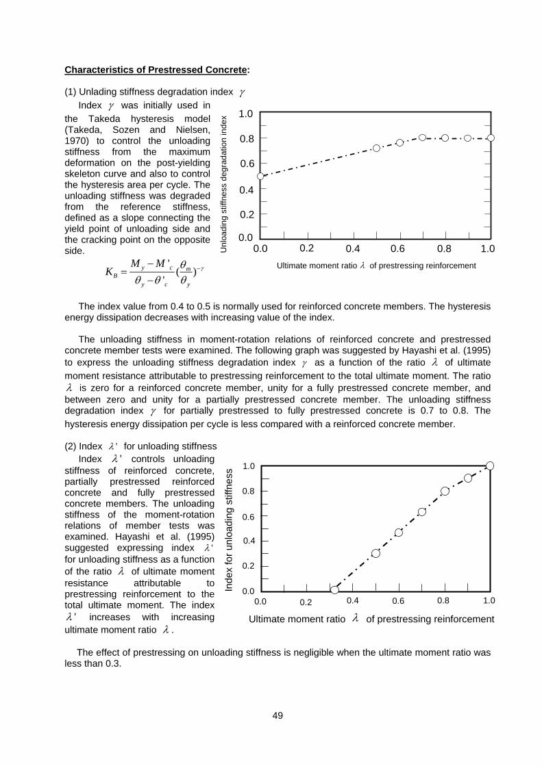
49
Characteristics of Prestressed Concrete: (1) Unlading stiffness degradation index γ
Index γ was initially used in the Takeda hysteresis model (Takeda, Sozen and Nielsen, 1970) to control the unloading stiffness from the maximum deformation on the post-yielding skeleton curve and also to control the hysteresis area per cycle. The unloading stiffness was degraded from the reference stiffness, defined as a slope connecting the yield point of unloading side and the cracking point on the opposite side.
'
( )'
y c mB
y c y
M MK γθ
θ θ θ−−
=−
The index value from 0.4 to 0.5 is normally used for reinforced concrete members. The hysteresis
energy dissipation decreases with increasing value of the index. The unloading stiffness in moment-rotation relations of reinforced concrete and prestressed
concrete member tests were examined. The following graph was suggested by Hayashi et al. (1995) to express the unloading stiffness degradation index γ as a function of the ratio λ of ultimate moment resistance attributable to prestressing reinforcement to the total ultimate moment. The ratio λ is zero for a reinforced concrete member, unity for a fully prestressed concrete member, and between zero and unity for a partially prestressed concrete member. The unloading stiffness degradation index γ for partially prestressed to fully prestressed concrete is 0.7 to 0.8. The hysteresis energy dissipation per cycle is less compared with a reinforced concrete member. (2) Index 'λ for unloading stiffness
Index 'λ controls unloading stiffness of reinforced concrete, partially prestressed reinforced concrete and fully prestressed concrete members. The unloading stiffness of the moment-rotation relations of member tests was examined. Hayashi et al. (1995) suggested expressing index 'λ for unloading stiffness as a function of the ratio λ of ultimate moment resistance attributable to prestressing reinforcement to the total ultimate moment. The index
'λ increases with increasing ultimate moment ratio λ .
The effect of prestressing on unloading stiffness is negligible when the ultimate moment ratio was less than 0.3.
0.0 0.2 0.4 0.6 0.8 1.0
1.0
0.0
0.2
0.4
0.6
0.8
Unl
oadi
ng s
tiffn
ess
degr
adat
ion
inde
x
Ultimate moment ratio of prestressing reinforcement λ
Inde
x fo
r unl
oadi
ng s
tiffn
ess
0.0 0.2 0.4 0.6 0.8 1.00.0
0.2
0.4
0.6
0.8
1.0
Ultimate moment ratio λ of prestressing reinforcement
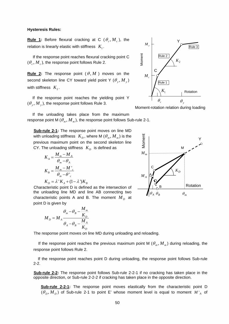
50
Hysteresis Rules: Rule 1: Before flexural cracking at C ( ,c cMθ ), the
relation is linearly elastic with stiffness 1K .
If the response point reaches flexural cracking point C ( ,c cMθ ), the response point follows Rule 2. Rule 2: The response point ( , Mθ ) moves on the second skeleton line CY toward yield point Y ( ,y yMθ )
with stiffness 2K .
If the response point reaches the yielding point Y ( ,y yMθ ), the response point follows Rule 3.
If the unloading takes place from the maximum
response point M ( ,m mMθ ), the response point follows Sub-rule 2-1. Sub-rule 2-1: The response point moves on line MD with unloading stiffness DK , where M ( ,m mMθ ) is the previous maximum point on the second skeleton line CY. The unloading stiffness DK is defined as
'
'' (1 ')
m AA
m A
m cB
m c
D A B
M MK
M MK
K K K
θ θ
θ θλ λ
−=
−−
=−
= + −
Characteristic point D is defined as the intersection of the unloading line MD and line AB connecting two characteristic points A and B. The moment DM at point D is given by
mm B
DD A
AA B
D
MKM M MK
θ θ
θ θ
− −=
− −
The response point moves on line MD during unloading and reloading. If the response point reaches the previous maximum point M ( ,m mMθ ) during reloading, the
response point follows Rule 2.
If the response point reaches point D during unloading, the response point follows Sub-rule 2-2. Sub-rule 2-2: The response point follows Sub-rule 2-2-1 if no cracking has taken place in the opposite direction, or Sub-rule 2-2-2 if cracking has taken place in the opposite direction.
Sub-rule 2-2-1: The response point moves elastically from the characteristic point D ( ,D DMθ ) of Sub-rule 2-1 to point E’ whose moment level is equal to moment 'AM of
C
Y
yθ cθ
cM
yM
Rotation
Mom
ent
1K
2K
Rule 1
Rule 2
Rule 3
Moment-rotation relation during loading
C
Rotation
AAM
M
mθ
B
DK
Y
D
Mom
ent
Bθ
mM
Aθ
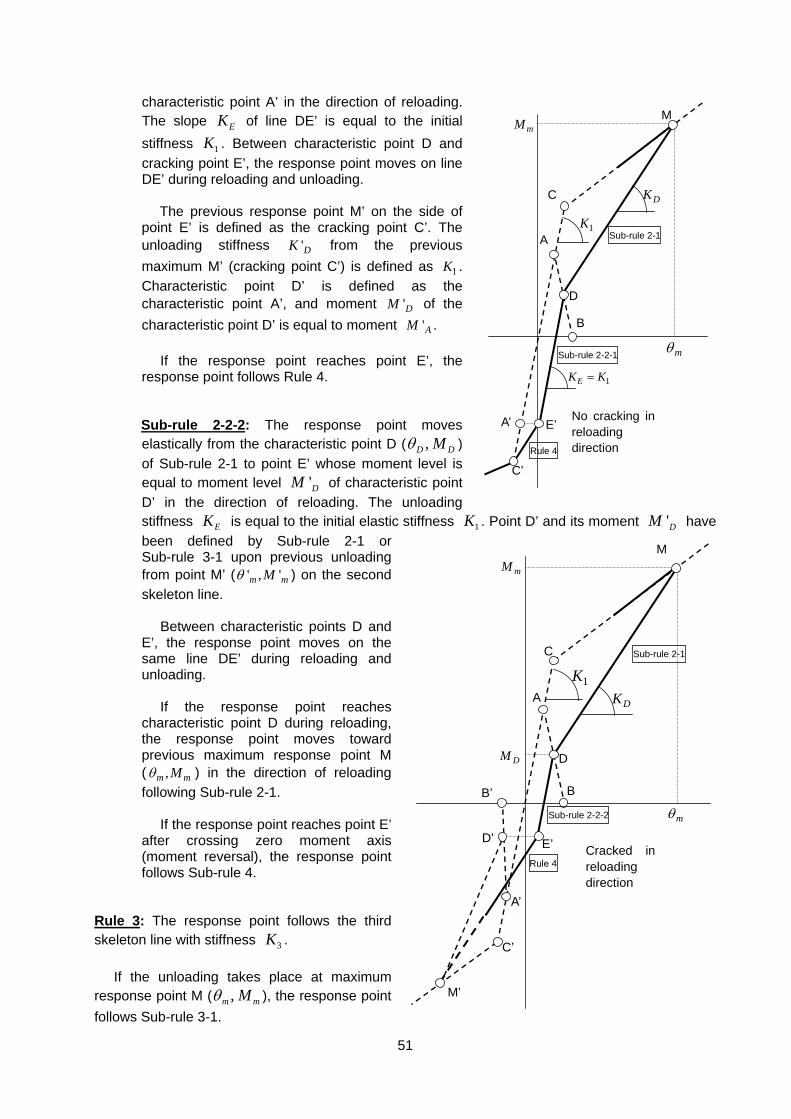
51
characteristic point A’ in the direction of reloading. The slope EK of line DE’ is equal to the initial stiffness 1K . Between characteristic point D and cracking point E’, the response point moves on line DE’ during reloading and unloading.
The previous response point M’ on the side of point E’ is defined as the cracking point C’. The unloading stiffness 'DK from the previous maximum M’ (cracking point C’) is defined as 1K . Characteristic point D’ is defined as the characteristic point A’, and moment 'DM of the characteristic point D’ is equal to moment 'AM .
If the response point reaches point E’, the response point follows Rule 4. Sub-rule 2-2-2: The response point moves elastically from the characteristic point D ( ,D DMθ ) of Sub-rule 2-1 to point E’ whose moment level is equal to moment level 'DM of characteristic point D’ in the direction of reloading. The unloading stiffness EK is equal to the initial elastic stiffness 1K . Point D’ and its moment 'DM have been defined by Sub-rule 2-1 or Sub-rule 3-1 upon previous unloading from point M’ ( ' , 'm mMθ ) on the second skeleton line.
Between characteristic points D and E’, the response point moves on the same line DE’ during reloading and unloading.
If the response point reaches
characteristic point D during reloading, the response point moves toward previous maximum response point M ( ,m mMθ ) in the direction of reloading following Sub-rule 2-1.
If the response point reaches point E’ after crossing zero moment axis (moment reversal), the response point follows Sub-rule 4.
Rule 3: The response point follows the third skeleton line with stiffness 3K .
If the unloading takes place at maximum response point M ( ,m mMθ ), the response point follows Sub-rule 3-1.
1K A
B
C
D
E’A’
C’
1EK K=
mθ
mM
No cracking in reloading direction
M
DK
Sub-rule 2-1
Sub-rule 2-2-1
Rule 4
1K
DK A
B
C
D
E’
A’
B’
C’
M’
D’Cracked in reloading direction
DM
mM
mθ
M
Sub-rule 2-1
Sub-rule 2-2-2
Rule 4
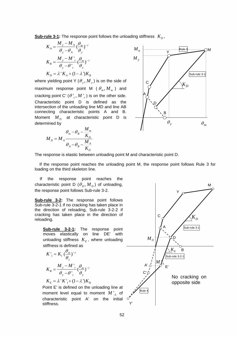
52
Sub-rule 3-1: The response point follows the unloading stiffness DK ,
( )
'( )
'
' (1 ')
y A mA
y A y
y c mB
y c y
D A B
M MK
M MK
K K K
γ
γ
θθ θ θ
θθ θ θ
λ λ
−
−
−=
−
−=
−
= + −
where yielding point Y ( ,y yMθ ) is on the side of
maximum response point M ( ,m mMθ ) and
cracking point C’ ( ' , 'c cMθ ) is on the other side. Characteristic point D is defined as the intersection of the unloading line MD and line AB connecting characteristic points A and B. Moment DM at characteristic point D is determined by
mm B
DD A
AA B
D
MKM M MK
θ θ
θ θ
− −=
− −
The response is elastic between unloading point M and characteristic point D.
If the response point reaches the unloading point M, the response point follows Rule 3 for loading on the third skeleton line.
If the response point reaches the characteristic point D ( ,D DMθ ) of unloading, the response point follows Sub-rule 3-2. Sub-rule 3-2: The response point follows Sub-rule 3-2-1 if no cracking has taken place in the direction of reloading, Sub-rule 3-2-2 if cracking has taken place in the direction of reloading.
Sub-rule 3-2-1: The response point moves elastically on line DE’ with unloading stiffness EK , where unloading stiffness is defined as
1 1
1
' ( )
'( )
'
' ' (1 ')
m
y
y c mB
y c y
E B
K K
M MK
K K K
γ
γ
θθ
θθ θ θ
λ λ
−
−
=
−=
−
= + −
Point E’ is defined on the unloading line at moment level equal to moment 'AM of characteristic point A’ on the initial stiffness.
A
C
Y
M
B
'AM
Y’
C’
D DM
DK
E’
EK
A’
No cracking on opposite side
Sub-rule 3-1
Sub-rule 3-2-1
Rule 4
C
Y M
A
D
B
DK
mθyθ
yM
uM
Sub-rule 3-1
Rule 3
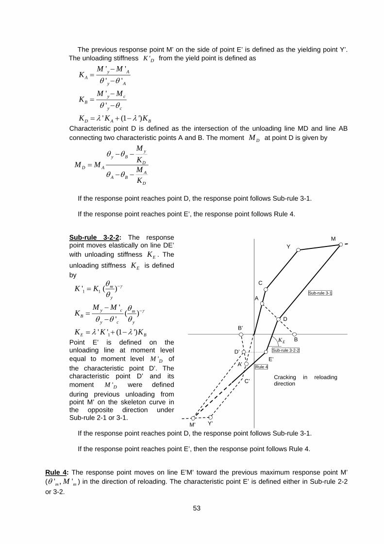
53
The previous response point M’ on the side of point E’ is defined as the yielding point Y’. The unloading stiffness 'DK from the yield point is defined as
' '' '
''
' (1 ')
y AA
y A
y cB
y c
D A B
M MK
M MK
K K K
θ θ
θ θ
λ λ
−=
−
−=
−
= + −
Characteristic point D is defined as the intersection of the unloading line MD and line AB connecting two characteristic points A and B. The moment DM at point D is given by
yy B
DD A
AA B
D
MKM M MK
θ θ
θ θ
− −=
− −
If the response point reaches point D, the response point follows Sub-rule 3-1. If the response point reaches point E’, the response point follows Rule 4.
Sub-rule 3-2-2: The response point moves elastically on line DE’ with unloading stiffness EK . The unloading stiffness EK is defined by
1 1
1
' ( )
'( )
'
' ' (1 ')
m
y
y c mB
y c y
E B
K K
M MK
K K K
γ
γ
θθ
θθ θ θ
λ λ
−
−
=
−=
−
= + −
Point E’ is defined on the unloading line at moment level equal to moment level 'DM of the characteristic point D’. The characteristic point D’ and its moment 'DM were defined during previous unloading from point M’ on the skeleton curve in the opposite direction under Sub-rule 2-1 or 3-1.
If the response point reaches point D, the response point follows Sub-rule 3-1. If the response point reaches point E’, then the response point follows Rule 4.
Rule 4: The response point moves on line E’M’ toward the previous maximum response point M’ ( ' , 'm mMθ ) in the direction of reloading. The characteristic point E’ is defined either in Sub-rule 2-2 or 3-2.
A
B
C
D
Y M
C’
A’
Y’M’
B’
D’E’
EK
Cracking in reloading direction
Sub-rule 3-1
Sub-rule 3-2-2
Rule 4
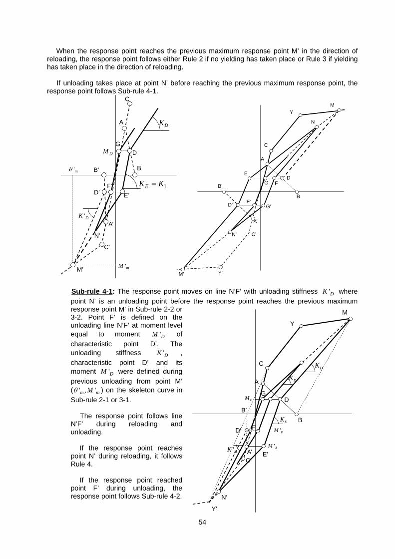
54
When the response point reaches the previous maximum response point M’ in the direction of reloading, the response point follows either Rule 2 if no yielding has taken place or Rule 3 if yielding has taken place in the direction of reloading.
If unloading takes place at point N’ before reaching the previous maximum response point, the
response point follows Sub-rule 4-1.
1EK K=
DKA
B
C
D
E’
A’
B’
C’
M’
D’
DM
F’
G
N’
'DK
'mM
'mθ
A
B
C
D
Y M
C’
A’
B’
D’
Y’M’
G’
E
N
F
N’
F’
G
Sub-rule 4-1: The response point moves on line N’F’ with unloading stiffness 'DK where point N’ is an unloading point before the response point reaches the previous maximum response point M’ in Sub-rule 2-2 or 3-2. Point F’ is defined on the unloading line N’F’ at moment level equal to moment 'DM of characteristic point D’. The unloading stiffness 'DK , characteristic point D’ and its moment 'DM were defined during previous unloading from point M’ ( ' , 'm mMθ ) on the skeleton curve in Sub-rule 2-1 or 3-1.
The response point follows line N’F’ during reloading and unloading.
If the response point reaches point N’ during reloading, it follows Rule 4.
If the response point reached
point F’ during unloading, the response point follows Sub-rule 4-2.
A
C
Y
M
B
'AM
'DM
B’
Y’
C’
D DM
DK
E’
EK
N’
A’'DK
D’
DK
F’
G
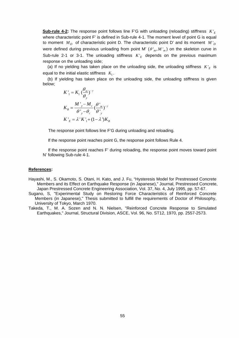
55
Sub-rule 4-2: The response point follows line F’G with unloading (reloading) stiffness 'EK where characteristic point F’ is defined in Sub-rule 4-1. The moment level of point G is equal to moment DM of characteristic point D. The characteristic point D’ and its moment 'DM were defined during previous unloading from point M’ ( ' , 'm mMθ ) on the skeleton curve in Sub-rule 2-1 or 3-1. The unloading stiffness 'EK depends on the previous maximum response on the unloading side;
(a) If no yielding has taken place on the unloading side, the unloading stiffness 'EK is equal to the initial elastic stiffness 1K .
(b) If yielding has taken place on the unloading side, the unloading stiffness is given below;
1 1
1
' ( )
' '( )' '
' ' ' (1 ')
m
y
y c mB
y c y
E B
K K
M MK
K K K
γ
γ
θθ
θθ θ θ
λ λ
−
−
=
−=
−
= + −
The response point follows line F’G during unloading and reloading.
If the response point reaches point G, the response point follows Rule 4.
If the response point reaches F’ during reloading, the response point moves toward point
N’ following Sub-rule 4-1.
References: Hayashi, M., S. Okamoto, S. Otani, H. Kato, and J. Fu, “Hysteresis Model for Prestressed Concrete
Members and its Effect on Earthquake Response (in Japanese),” Journal, Prestressed Concrete, Japan Prestressed Concrete Engineering Association, Vol. 37, No. 4, July 1995, pp. 57-67.
Sugano, S, "Experimental Study on Restoring Force Characteristics of Reinforced Concrete Members (in Japanese)," Thesis submitted to fulfill the requirements of Doctor of Philosophy, University of Tokyo, March 1970.
Takeda, T., M. A. Sozen and N. N. Nielsen, "Reinforced Concrete Response to Simulated Earthquakes," Journal, Structural Division, ASCE, Vol. 96, No. ST12, 1970, pp. 2557-2573.
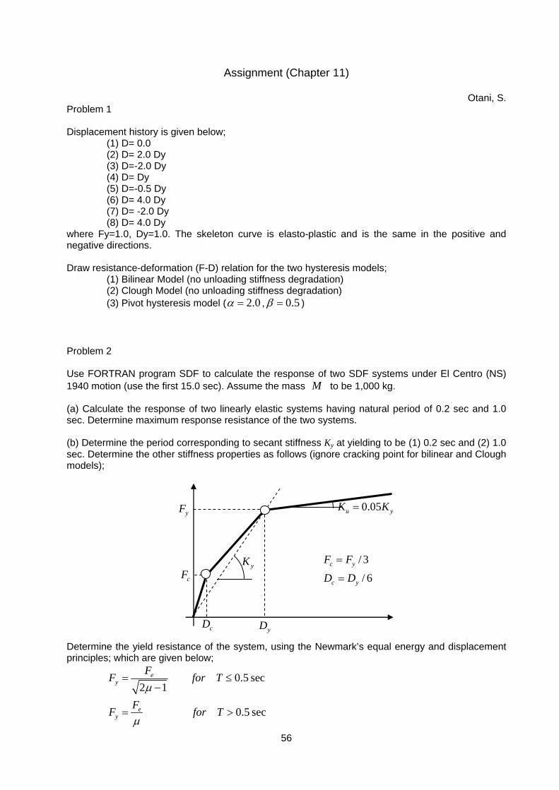
56
Assignment (Chapter 11)
Otani, S. Problem 1 Displacement history is given below; (1) D= 0.0 (2) D= 2.0 Dy (3) D=-2.0 Dy (4) D= Dy (5) D=-0.5 Dy (6) D= 4.0 Dy (7) D= -2.0 Dy (8) D= 4.0 Dy where Fy=1.0, Dy=1.0. The skeleton curve is elasto-plastic and is the same in the positive and negative directions. Draw resistance-deformation (F-D) relation for the two hysteresis models; (1) Bilinear Model (no unloading stiffness degradation) (2) Clough Model (no unloading stiffness degradation) (3) Pivot hysteresis model ( 2.0α = , 0.5β = ) Problem 2 Use FORTRAN program SDF to calculate the response of two SDF systems under El Centro (NS) 1940 motion (use the first 15.0 sec). Assume the mass M to be 1,000 kg. (a) Calculate the response of two linearly elastic systems having natural period of 0.2 sec and 1.0 sec. Determine maximum response resistance of the two systems. (b) Determine the period corresponding to secant stiffness Ky at yielding to be (1) 0.2 sec and (2) 1.0 sec. Determine the other stiffness properties as follows (ignore cracking point for bilinear and Clough models);
0.05u yK K=
yKcF
yF
cD yD
/ 3
/ 6c y
c y
F F
D D
=
=
Determine the yield resistance of the system, using the Newmark’s equal energy and displacement principles; which are given below;
0.5 sec2 1
0.5 sec
ey
ey
FF for T
FF for T
μ
μ
= ≤−
= >

57
where, eF : maximum resistance of a linearly elastic system having the same initial (yield) period, and μ : allowable ductility factor (=4.0), defined as the allowable maximum deformation divided by the yield displacement. (c) Calculate the response of bilinear model (ignore the cracking point), Clough model (ignore the cracking point), and Takeda model. Plot the resistance-deformation relation during the earthquake for each model. Compare the response displacement waveforms of the three models. Damping should be proportional to instantaneous stiffness, and the damping factor should be 0.05 for the yield secant stiffness.
2 y
chM K
=
(d) Compare the response displacement waveforms of Clough model using damping proportional to stiffness and damping proportional to mass. The damping factor of the two cases should be 0.05 at the initial stage. Problem 3 Use FORTRAN program Pivot. Use the same stiffness properties of the Clough model in Problem 3. Study the effect of post-yielding stiffness on the response, by varying the post yielding stiffness uK ,
(1) 0.10u yK K= , (2) 0.0uK = , and (3) 0.10u yK K= − . The third and fourth point of resistance-deformation relation can be selected on the post-yielding branch. Plot the resistance-deformation relation for each case, and compare response displacement waveforms of the three cases. The parameters of the Pivot model should be 2.0α = and 1/ 3β = .