hysteretic co2 sorption in a novel copper(ii)-indazole ... · hysteretic co. 2. sorption in a novel...

Hysteretic CO2 sorption in a novel copper(II)-indazole-carboxylate porous coordination polymer

Chris S Hawes*, Ravichandar Babarao, Matthew Hill, Keith White, Brendan F. Abrahams and Paul E. Kruger*

Electronic Supporting Information (ESI)

Electronic Supplementary Material (ESI) for Chemical CommunicationsThis journal is © The Royal Society of Chemistry 2012

Experimental

General Considerations

All synthetic transformations were carried out using commercially available reagents and starting

materials, and were carried out in air unless otherwise specified. Anhydrous solvents were prepared

by passing HPLC-grade solvent through a sealed column of activated alumina. NMR spectra were

collected on a Varian INOVA spectrometer operating at 500 MHz for 1H and 125 MHz for 13C nuclei,

and are referenced to the residual solvent peaks. Mass spectra were collected on a Bruker MaXis 4G

Electrospray mass spectrometer operating in positive ion mode. Melting points were collected on an

Electrothermal melting point apparatus and are uncorrected. Thermogravimetric analyses were carried

out on an Alphatec Q600 SDT TGA/DSC instrument using alumina crucibles, where samples were

heated at a rate of 1 °C/hr to 500 °C under a nitrogen flow of 100 mL/min. Infrared spectra were

recorded on a Perkin-Elmer Spectrum One FTIR spectrometer operating in diffuse reflectance mode,

with samples prepared as KBr mulls. Microanalysis was carried out at the Campbell Microanalytical

Laboratory, University of Otago, New Zealand. Solvothermal reactions were carried out within Parr

Instruments Teflon lined acid digestion bombs within Carbolite PF60 ovens utilising Eurotherm

temperature controllers.


Synthesis of H2L.

NO2

O OH

NO2

O O

NH2

O O O OH

HN N

(i) (ii) (ii i), (iv)

a

b

c

d

e

f93% 83% 47%

HL1

Scheme S1: Reagents and conditions: (i) MeOH, H2SO4 (cat.), reflux 16 hr; (ii) 10% Pd/C,

NH4HCO2, MeOH, RT 3 hr; (iii) Ac2O, KOAc, isoamyl nitrite, PhMe, reflux 16 hr; (iv) LiOH,

THF/H2O, reflux 48 hr, then HCl(aq).

Synthesis of methyl 3-methyl-4-nitrobenzoate, 1

To 3-methyl-4-nitrobenzoic acid (5 g; 28 mmol) in 30 mL methanol was added concentrated sulfuric

acid (2 mL) dropwise with vigorous stirring. The resulting mixture was refluxed overnight and

allowed to cool to room temperature, and then concentrated under reduced pressure. The residue was

combined with 100 mL distilled water and extracted several times with dichloromethane, and the

organic phases were combined, washed with water, dried with MgSO4 and evaporated to dryness to

give the product as a white solid. Yield 5.0 g (93%). Analytical data were found to be consistent with

the commercially available material.

Synthesis of methyl 3-methyl-4-aminobenzoate, 2

The title compound was synthesised by an adaptation of the method reported by Ehrenkaufer [1].

Methyl 3-methyl-4-nitrobenzoate (2 g; 10 mmol) was dissolved in 20 mL anhydrous methanol under a

nitrogen atmosphere, to which was added 10% palladium on activated carbon (500 mg) with stirring.

To this mixture was added ammonium formate (3 g; 48 mmol) in one portion, and the mixture was

vigorously stirred at room temperature until exothermicity and gas evolution was seen to cease (3

hours). The mixture was filtered through celite, washed with several portions of methanol, and the

filtrates combined and evaporated. The residue was slurried in distilled water, and the solids were

filtered and dried in vacuo to give the product as a white solid. Yield 1.4 g (83%). Analytical data

were found to be consistent with literature values [2].

1 2 H2L


Synthesis of 1H-indazole-5-carboxylic acid, H2L

The title compound was prepared by an adaptation to the method reported by Hassmann [3]. To 40

mL dry toluene under a nitrogen atmosphere was added methyl 3-methyl 4-aminobenzoate (1.3 g, 7.9

mmol) and potassium acetate (400 mg, 4.1 mmol), and the mixture was heated to reflux, at which time

acetic anhydride (2.3 mL, 25 mmol) was added, and the mixture was stirred at temperature for 10

minutes. Isoamyl nitrite (1.7 mL, 13 mmol) was added over 30 minutes, and the mixture was refluxed

overnight. On cooling, the mixture was filtered and evaporated to dryness, to give an orange solid,

which was filtered and washed with petroleum ether, giving 1.44g of methyl N-acetyl indazole-5-

carboxylate. This material was taken up in 50 mL THF and added to a solution of lithium hydroxide

(7 g, 290 mmol) in 50 mL water, and the resulting mixture was refluxed for 48 hours. On cooling, the

mixture was concentrated on a rotary evaporator to remove THF, and the aqueous phase was filtered

and taken to pH 4 with dilute hydrochloric acid, causing precipitation of the product, which was

filtered, washed with water and dried in vacuo. Yield 600 mg (47%). MP 297–301 °C (decomp.);

δH(500 MHz, d6-DMSO): 7.60 (d, 1H, J = 8.8 Hz, Hf), 7.91 (dd, 1H, J1= 8.8 Hz, J2= 1.6 Hz, He), 8.24

(d, 1H, J = 0.8 Hz, Hb), 8.45 (dd, 1H, J1 = 1.3 Hz, J2 = 0.8 Hz, Hc), 13.2 (br s, 2H, Hd + Ha); δc(125

MHz, d6-DMSO): 110.2, 122.7, 123.2, 123.9, 126.7, 135.3, 141.8, 167.8; m/z (ESMS): 163.0504

[M+H+], calculated for C8H7N2O2 163.0502; υmax(KBr)/cm-1 3297 s br, 2504 m br, 1686 s, 1622 m,

1469 w, 1357 m, 1319 s, 1269 s, 1203 m, 1134 m, 1080 m, 948 s, 768 s.

Synthesis of poly-catena-[Cu(HL)2], 1

H2L (10 mg; 61 µmol) was combined with Cu(NO3)2·3H2O (4 mg; 16 µmol) and (NH4)2SiF6 (5 mg;

28 µmol) in a 1:1 MeOH/H2O mixture (2 mL), and added to a 23 mL Parr Instruments acid digestion

bomb, which was heated to 100 °C, allowed to dwell for 24 hours, and cooled to room temperature at

4 °C/hr. The purple crystals obtained were filtered and washed sequentially with methanol, water, and

a further portion of methanol, and were air dried. Yield 3.6 mg (59%); MP >300 °C; Found C, 48.6;

H, 2.86; N, 13.5; C48H30N12O12Cu3·2MeOH·H2O requires C, 48.4; H, 3.30; N, 13.6 %;

υmax(KBr)/cm-1 3250 m; 1817 w, 1633 m, 1599 s, 1570 s, 1513 m, 1458 m, 1380 s, 1273 m, 1133 m,

1083 s, 971 s, 857 s, 793 s, 781 s, 597 m.


Figure S1: 1H NMR spectrum of H2L (d6-DMSO @ 500 MHz):

L1 1H NMR.esp

13.5 13.0 12.5 12.0 11.5 11.0 10.5 10.0 9.5 9.0 8.5 8.0 7.5 7.0Chemical Shift (ppm)

0.1

0.2

0.3

0.4

0.5

0.6

0.7

0.8

0.9

1.0

1.1

Nor

mal

ized

Inte

nsity

Figure S2: 13C NMR spectrum of H2L (d6-DMSO @ 125 MHz):

L1 13C.esp

175 170 165 160 155 150 145 140 135 130 125 120 115 110 105Chemical Shift (ppm)

0

0.5

1.0

1.5

2.0

2.5

3.0

Nor

mal

ized

Inte

nsity

a

bcd

ef

NN

H

OH

O

a

bcd

ef

NN

H

OH

O

b

c

a; d

e

f


X-ray Crystallography

Refinement data are presented in Table S1. X-ray crystallographic data collection and refinement was

carried out with an Oxford ATLAS area detector using Cu/Kα radiation from an Oxford SuperNova

dual microsource instrument (λ = 1.5418 Å). All structures were solved using direct methods with

SHELXS [4] and refined on F2 using all data by full matrix least-squares procedures with SHELXL-

97 [5] within OLEX-2 [6].. Non-hydrogen atoms were refined with anisotropic displacement

parameters. Hydrogen atoms were included in calculated positions with isotropic displacement

parameters 1.2 times the isotropic equivalent of their carrier atoms. The functions minimized were

Σw(F2o-F2

c), with w=[σ2(F2o)+aP2+bP]-1, where P=[max(Fo)2+2F2

c]/3.

Structure solution revealed the presence of channels within 1. The electron density present in these

channels was so diffuse as to prevent explicit modelling of the solvent guests, and the use of the

SQUEEZE routine within PLATON [7] was not required due to the high degree of accuracy evident

in the unmodified data. However, SQUEEZE was used to estimate the void contents on electron

density grounds and suggested 427 electrons per unit cell, equivalent to approximately 47 electrons

per copper, consistent with the equivalent of 2.5 methanol molecules, 4.5 water molecules, or a

combination of the two, and accounting for ca. 36% of the unit cell volume. The structure of 1 after

heating (designated 1A), returned near identical crystallographic data to 1 (Table S1). However the

void contents calculated by SQUEEZE were reduced to 37 electrons per unit cell and with markedly

improved refinement statistics, suggesting significant desolvation of the channels whilst maintaining

the open network structure.


Table S1 Crystallographic data for 1 and 1A

Compound reference 1 1A Chemical formula C16H10CuN4O4 C16H10CuN4O4 Formula Mass Crystal System

385.82 Trigonal

385.82 Trigonal

a/Å 33.6525(6) 33.6966(8) b/Å 33.6525(6) 33.6966(8) c/Å 4.80132(11) 4.78817(13) α/° 90.00 90.00 β/° 90.00 90.00 γ/° 120.00 120.00 Unit cell volume/Å3 4708.98(16) 4708.4(2) Temperature/K 120.0(1) 120.0(1) Space group R3̄ R3̄ No. of formula units per unit cell, Z 9 9 No. of reflections measured 26227 9622 No. of independent reflections 1883 2092 Rint 0.0274 0.0221 Final R1 values (I > 2σ(I)) 0.0379 0.0265 Final wR(F2) values (I > 2σ(I)) 0.1331 0.0697 Final R1 values (all data) 0.0396 0.0284 Final wR(F2) values (all data) µ /mm-1

0.1348 1.686

0.0711 1.686

Table S2: Hydrogen bond parameters for 1.

D–H...A d(D–H)/Å d(H–A)/Å d(D–A)/Å D–H...A/°

N3–H3...O13i 0.860(18) 1.99(3) 2.721(2) 143(3)

Symmetry operator: i) +X, +Y, 1+Z

Table S3: Hydrogen bond parameters for 1A.

D–H...A d(D–H)/Å d(H–A)/Å d(D–A)/Å D–H...A/°

N3–H3...O13i 0.847(15) 1.970(17) 2.7219(15) 147.3(18)

Symmetry operator: i) 1-X, 1-Y, 1-Z


Figure S3: Schematic view of the two interpenetrated networks in 1 viewed approximately down the

crystallographic c-axis, choosing Cu(II) centres as nodes.


Figure S4: Thermogravimetric analysis trace for 1 showing weight % (green) and δW/δT (blue).


Figure S5: X-ray Powder Diffraction Pattern for freshly prepared 1 (red), dehydrated sample 1A

(green) and pattern simulated from single crystal data (blue).

-100

100

300

500

700

900

1100

1300

1500

5 15 25 35 45

Inte

nsity

(A.U

.)

2θ (°)

1A

1

Predicted


Gas sorption experimental and isosteric heat of sorption calculations

A sample of 1 was baked at 150 °C under dynamic vacuum overnight. The dried sample on which the

gas sorption studies were undertaken had a mass of 103.6 mg. Between isotherm measurements the

sample was re-baked at 150 °C for 2 hours.

Gas sorption data were measured using a Sieverts-type BELsorp-HP automatic gas sorption apparatus

(BEL Japan Inc.). Ultra-high purity CH4, CO2, and He were used for the sorption studies.

Corrections were made for non-ideal gas behaviour at high pressures of each gas at each measurement

and reference temperature. Source data were obtained from the NIST fluid properties website. [8]

Sample compartment temperatures between 258 K and 298 K were controlled by a Julabo F25-ME

chiller/heater. A calibrated external Pt100 temperature probe monitored the flask temperature.

Samples were kept at the measurement temperature for a minimum of 1 hr after the desired

temperature had been achieved to allow thermal equilibrium to be attained before data measurement

commenced.

Isosteric heats of sorption were calculated using least-squares fitting of a virial-type thermal

adsorption equation that modelled lnP as a function of amount of surface excess of gas sorbed over all

measurement temperatures. [9]


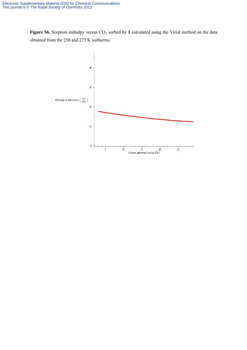
Figure S6. Sorption enthalpy versus CO2 sorbed by 1 calculated using the Virial method on the data

obtained from the 258 and 273 K isotherms.


Figure S7. 273K isotherms for CO2 (yellow diamonds) and methane (black circles) sorption by 1.

Figure S8. H2 Isotherms collected at 258K (blue circles), and 273K (red squares)

0

5

10

15

20

0 500 1000 1500 2000 2500 3000 3500

Vol s

orbe

d (c

m3 (

STP)

/g)

P/kPa

273 K

258 K


Figure S9. N2 isotherm collected at 77K

Figure S10. High-resolution CO2 isotherm @ 273 K.

0

1

2

3

4

5

0 20 40 60 80 100

Vol s

orbe

d (c

m3

(STP

) /g)

P/kPa

77 K


Simulation Methods and Models

The adsorption of pure CO2 was simulated by grand canonical Monte Carlo (GCMC) method.

Because the chemical potentials of adsorbate in adsorbed and bulk phases are identical at

thermodynamic equilibrium, GCMC simulation allows one to relate the chemical potentials of

adsorbate in both phases and has been widely used for the simulation of adsorption. The framework

atoms are kept frozen during simulation. The LJ interactions were evaluated with a spherical cutoff

equal to half of the simulation box with long-range corrections added; the Coulombic interactions

were calculated using the Ewald sum method. The number of trial moves in a typical GCMC

simulation was 2 × 107, though additional trial moves were used at high loadings. The first 107 moves

were used for equilibration and the subsequent 107 moves for ensemble averages. Five types of trial

moves were attempted in GCMC simulation, namely, displacement, rotation, and partial regrowth at a

neighboring position, entire regrowth at a new position, and swap with reservoir. Unless otherwise

mentioned, the uncertainties are smaller than the symbol sizes in the figures presented.

Experimental adsorption isotherm is usually reported in the excess amount exN while simulation

gives the absolute amount abN . To convert from abN to exN , we use

freebabex VNN ρ−= (1)

where bρ is the density of bulk adsorbate calculated using Peng-Robinson equation of state, freeV is

the free volume in adsorbent available for adsorption and is estimated from

[ ]∫ −=V

BHeadfree drTkruV /)(exp (2)

where Headu is the interaction between Helium and adsorbent, in which Heσ = 2.58 Å and

BHe k/ε =10.22 K.10 Note that the free volume detected by helium is temperature dependent, and

usually the room temperature is chosen. The ratio of free volume freeV to the occupied volume totalV

gives the porosity φ of adsorbent.

Canonical ensemble (NVT) simulation is performed to estimate the isosteric heat of adsorption

at infinite dilution. A single adsorbate molecule is subjected to three types of trial moves employed in

the NVT simulation, namely, translation, rotation and regrowth. The isosteric heat at infinite dilution

is calculated from

(3)

where is the total adsorption energy of a single molecule with adsorbent and is the

intramolecular interaction of a single gas molecule in bulk phase.

The adsorbate CO2 was mimicked as three-site model to account for the quadrupole moment.

The C−O bond length in CO2 was 1.18 Å and the bond angle ∠OCO was 180°. The charges on C and

( )0 0 0st total intra= − −q RT U U

0totalU 0

intraU


O atoms were +0.576e and –0.288e (e = 1.6022 ×10-19 C the elementary charge), resulting in a

quadrupole moment of −1.29 × 10-39 C⋅m2. The LJ parameters for CO2 were σC = 2.789 Å, εC = 29.66

K, σO = 3.011 Å, εO = 82.96 K.11

The experimentally determined crystal structure was used in simulations. Atomic partial

charges are calculated based on fragmental cluster using density functional theory (DFT) as

implemented in DMol3.12 The DFT calculation was performed on a cluster model cleaved from the

unit cell. The PW91 functional along with the Double-ξ numerical polarization (DNP) basis set was

used in the DFT calculations, which is comparable to 6-31G(d,p) Gaussian-type basis set. DNP basis

set incorporates p-type polarization into hydrogen atoms and d-type polarization into heavier atoms.

From the DFT calculations, the atomic charges were evaluated by fitting to the electrostatic potential

using the Merz-Kollman (MK) scheme as listed in Table S4.13,14 The interactions of gas-adsorbent

and gas-gas were modeled as a combination of pairwise site-site Lennard-Jones (LJ) and Coulombic

potentials. The LJ potential parameters of the framework atoms are adopted from and Dreiding force

field.15 However, the DREIDING force field parameter is not available for Cu atom, thus the

parameter from the Universal force field (UFF)16 was adopted. To account for inflection in CO2

isotherm the DREIDING force field parameters were rescaled to match the experimental isotherm.

This type of adjustment of force field parameters has been widely done in previous works.17-19 Table

S5 lists the set of LJ parameters used in this study. The Lorentz-Berthelot combining rules were used

to calculate the cross LJ interaction parameters.

Table S4. Atom charges in 1 and the atom types are labelled in Figure S11.

Atom Type Cu1 N2 N3 O12 O13 C4

Charge 0.918 -0.238 -0.226 -0.690 -0.604 0.236

Atom Type C5 C6 C7 C8 C9 C10

Charge -0.363 -0.040 -0.056 -0.322 0.116 -0.116

Atom type C11 H3 H5 H6 H8 H10

Charge 0.684 0.346 0.219 0.174 0.219 0.202


Figure S11. Atomic types in 1.

Table S5. LJ potential parameter for the framework atoms in 1.

Atom type Cu C O N

H

(A)σ

3.11 3.30 2.88 3.10 2.71

B/ (K)kε 2.52 39.9 40.2 29.2 6.38

Cu1

N2 N3

O12 O13

C5 C7

C8 C9

C10

C11

H3

H5

H6

H8

H10

C4

C6


Results and Discussions

Figure S12 shows the adsorption isotherm for CO2 at 298 K in 1. The simulated results agree fairly

well with the experimental data over the entire pressure.

Figure S12. Adsorption isotherm of CO2 in 1 at 298 K in (a) log scale (b) linear scale

To better understand the location of adsorption sites, Figure S13 shows the radial distribution

functions g(r) between CO2 and the framework atoms in 1.

ji

ijij NrNr

VNrg

∆∆

= 24)(

π

where r is the distance between species i and j, ijN∆ is the number of species j around i within a shell

from r to r + Δr, V is the volume, N i and Nj are the number of species i and j. A pronounced peak in

g(r) is observed at r = 4.2 Å between CO2 and framework atoms C5 and C6. This confirms that CO2

interacts with the phenyl ring more strongly than the other framework atoms. The isosteric heat of

adsorption predicted from simulation is around -15 kJ/mol at zero loading which is slightly lower than

the experimentally observed value of -17.5 kJ/mol.

P (kPa)1 10 100 1000

Load

ing

cc(S

TP)/g

0

20

40

60

80

100ExperimentSimulation

P (kPa)500 1000 1500 2000 2500 3000

0

20

40

60

80

100ExperimentSimulation

(a) (b)


Figure S13. Radial distribution functions between CO2 and framework atoms (a) C5 and C6 (b) Cu1,

N2, N3, O12 and O13.

Figure S14 shows the density contours of CO2 at 10 kPa in 1. The contours are viewed from

the (100) plane and generated by accumulating 200 equilibrium configurations. CO2 molecules are

primarily adsorbed in the pore centres.

Figure S14. Density contours of CO2 adsorption at 10 kPa in 1.

r(Å)0 5 10 15 20 25

g (r

)

0.0

0.5

1.0

1.5

2.0

2.5CO2- C5

CO2- C6

r(Å)0 5 10 15 20 25

0.0

0.5

1.0

1.5

2.0

2.5CO2- Cu

CO2- N2

CO2- N3

CO2- O12

CO2- O13

(a) (b)


References

[1] S. Ram and R. E. Ehrenkaufer, Tetrahedron Lett., 1984, 25, 3415-3418

[2] G. Bartoli, M. Bosco, R. D. Pozzo and M. Petrini, Tetrahedron, 1987, 43, 4221-4226.

[3] C. Rüchardt and V. Hassmann, Liebigs Ann. Chem., 1980, 908-927.

[4] G.M. Sheldrick, Acta Crystallogr., Sect. A., 2008, 64, 112.

[5] G.M. Sheldrick, SHELXL-97, Programs for X-ray Crystal Structure Refinement, University of

Gottingen, 1997.

[6] O.V. Dolomanov, L.J. Bourhis, R.J. Gildea, J.A.K. Howard and H. Puschmann, OLEX2: A

complete structure solution, refinement and analysis program J. Appl. Cryst., 2009, 42, 339-

341.

[7] A. L. Spek, Acta Crystallogr. Sect. D- Biol. Crystallogr. 2009, 65, 148-155.

[8] http://webbook.nist.gov/chemistry/fluid/

[9] L. Czepirski, J. Jagiello, Chem. Eng. Sci. 1989, 44, 797–801

[10] Hirschfelder, J. O.; Curtiss, C. F.; Bird, R. B. Molecular Theory of Gases and liquids; John

Wiley: New York, 1964.

[11] Hirotani, A.; Mizukami, K.; Miura, R.; Takaba, H.; Miya, T.; Fahmi, A.; Stirling, A.; Kubo,

M.; Miyamoto, A. Appl. Surf. Sci. 1997, 120, 81-84.

[12] Materials Studio, 6.0 ed.; Accelrys, San Diego, 2011.

[13] Singh, U. C.; Kollman, P. A. J. Comput. Chem. 1984, 5, 129-145.

[14] Besler, B. H.; Merz, K. M.; Kollman, P. A. J. Comput. Chem. 1990, 11, 431-439.

[15] Mayo, S. L.; Olafson, B. D.; Goddard, W. A. J. Phys. Chem. 1990, 94, 8897-8909.

[16] Rappe, A. K.; Casewit, C. J.; Colwell, K. S.; Goddard, W. A.; Skiff, W. M. J. Am. Chem. Soc.

1992, 114, 10024-10035.

[17] Dubbeldam, D.; Calero, S.; Vlugt, T. J. H.; Krishna, R.; Maesen, T. L. M.; Beerdsen, E.; Smit,

B. Phys. Rev. Lett. 2004, 93.

[18] Thornton, A. W.; Dubbeldam, D.; Liu, M. S.; Ladewig, B. P.; Hill, A. J.; Hill, M. R. Energy

Environ. Sci. 2012, 5, 7637-7646.

[19] Zhang, W.; Huang, H.; Zhong, C.; Liu, D. PhysChemChemPhys 2012, 14, 2317-2325.


http://webbook.nist.gov/chemistry/fluid/

hysteretic co2 sorption in a novel copper(ii)-indazole ... · hysteretic co. 2. sorption in a novel...

Documents