I 1 I

A S S E S S ~ ~ N T OF A BOUNDARY 1 -'LAYER ANALYSIS PREDICT HEAT TRANSFER FLOW FIELD IN A TURBINE PASSAGE

bY I

I

O.L. Anderson ~ _ ~ _ _ _ _ _ _ _ _ _ ~ - - ~~ - -~

( b A S A - C E - 1 7 4 E 5 4 ) ASSESSf lEbl C t A 3-D m a - 3 ~ ~ 6 6 t C G f i D A B 1 L A P E E A h A I l S I E T C E E E 1 ; l C T BEAT Z f i A L S P k R A N C ELCY E l E L E It4 A IILliEIbE PASSAGE k l r i a l A A d . i y E 1 E S e F G r t ( U n i t€;d l c c h n o l o q i e s Unclas Eesearch C e n t e r ) 93 F CSCL 20D G3/34 0167350

I Prepared for: I t

National Aeronautics and Sp j 1 1 / j !

bwis Research Center

NASA Contract NAS3-2371L _ _ _ ~ ,

' \ -- -L __ ..-- L

necticut 06108

https://ntrs.nasa.gov/search.jsp?R=19880020682 2018-07-21T07:08:37+00:00Z

R85-956834

Assessment of a 3-D Boundary Layer Analys is t o P r e d i c t Heat T r a n s f e r and Flow F i e l d i n a Turbine Passage

TABLE OF CONTENTS

Page

1.0 S U M M A R Y . . . . . . . . . . . . . . . . . . . . . . . . . . . . . . 1

2.0 INTRODUCTION . . . . . . . . . . . . . . . . . . . . . . . . . . . 2

3.0 ANALYSIS . . . . . , . . . . . . . . . . . . . . . . . . . . . . . 5

3 . 1 3.2 3.3 3.4 3.5 3.6 3 . 7 3.8 3.9 3.10 3.11

Surface Coordinate System . . . . . . . . . . . . . . . . . . 5 Boundary Layer Equat ions . . . . . . . . . . . . . . . . . . 8 Normalized Equat ions . . . . . . . . . . . . . . . . . . . . 1 3 Genera l ized Levy - Lees Transformation . . . . . . . . . . . 1 5 P r o p e r t i e s of Boundary Layer Equat ions . . . . . . . . . . . 25 Boundary Condit ions . . . . . . . . . . . , . . . . . . . . . 25 Inf low Condit ions . . . . . . . . . . . . . . . . . . . . . . 27 Turbulence Model . . . . . . . . . . . . . . . . . . . . . . 32 F i n i t e D i f f e rence Equat ions . . . . . . . . . . . . . . . . . 34

Surface Euler Equat ions . . . . . . . . . . . . . . . . . . . 41 Genera l ized Sur face Coordinates . . . . . . . . . . . . . . . 35

4.0 RESULTS AND DISCUSSION . . . . . . . . . . . . . . . . . . . . . . 51

4.1 In t roduc to ry Discuss ion . . . . . . . . . . . . . . . . . . . 5 1 4.2 Turbine Cascade P res su re Surface . . . . . . . . . . . . . . . 52 4 . 3 Turbine Cascade Endwall Surface . . . . . . . . . . . . . . . 52 4.4 Turbine Cascade Suc t ion Surface . . . . . . . . . . . . . 54 4.5 Turbine Rotor P res su re Surface . . . . . . . . . . . . . . . . 55

5.0 CONCLUDING REMARKS . . . . . . . . . . . . . . . . . . . . . . . . 57

6.0 ACKNOWLEDGEMENT . . . . . . . . . . . . . . . . . . . . . . . . . . 58

7.0 REFERENCES . . . . . . . . . . . . . . . . . . . . . . . . . . . . 59

8.0 LIST OF SYMBOLS . . . . . . . . . . . . . . . . . . . . . . . . . . 61

9.0 FIGURES AND TABLES . . . . . . . . . . . . . . . . . . . . . . . . 65

10.0 APPENDIX - BOUNDARY LAYER PARAMETERS . . . . . . . . . . . . . . . 90

R85-956834

1 I I

Assessment of a 3-D Boundary Layer Analys is t o P r e d i c t Heat T rans fe r and Flow F i e l d i n a Turbine Passage

1.0 SUMMARY

An assessment has been made of t h e a p p l i c a b i l i t y of a t h r e e dimensional boundary l a y e r a n a l y s i s t o t h e c a l c u l a t i o n of hea t t r a n s f e r , t o t a l p r e s s u r e l o s s e s , and s t r e a m l i n e flow p a t t e r n s on t h e s u r f a c e s of both s t a t i o n a r y and r o t a t i n g t u r b i n e passages . I n support of t h i s e f f o r t , an a n a l y s i s has been devel- oped t o c a l c u l a t e a gene ra l nonorthogonal su r face coord ina te system f o r a r b i t r a r y t h r e e dimensional s u r f a c e s and a l s o t o c a l c u l a t e t h e boundary l a y e r edge condi- t i o n s f o r compressible flow us ing t h e s u r f a c e Euler equat ions and exper imenta l p re s su re d i s t r i b u t i o n s . Using a v a i l a b l e exper imenta l d a t a t o c a l i b r a t e t h e method, c a l c u l a t i o n s are presented f o r t h e p re s su re , endwall , and s u c t i o n su r - f aces of a s t a t i o n a r y cascade and f o r t h e p re s su re s u r f a c e of a r o t a t i n g t u r b i n e b lade . The r e s u l t s s t r o n g l y i n d i c a t e t h a t t he t h r e e dimensional boundary l a y e r a n a l y s i s can g ive good p r e d i c t i o n s of t h e flow f i e l d , l o s s , and hea t t r a n s f e r on the p r e s s u r e , s u c t i o n , and endwall s u r f a c e of a gas t u r b i n e passage.

1

R85-956834

2 . 0 INTRODUCTION

The p r e d i c t i o n of t h e complete flow f i e l d i n a t u r b i n e passage is an extremely d i f f i c u l t t a s k due t o t h e complex three-dimensional f low p a t t e r n which con ta ins s e p a r a t i o n and at tachment l i n e s , a sadd le p o i n t , and a horseshoe vo r t ex (F ig . 1 ) . Whereas, i n p r i n c i p a l such a problem can be so lved us ing f u l l Navier- Stokes equa t ions , i n r e a l i t y methods based on a Navier-Stokes s o l u t i o n procedure encounter d i f f i c u l t y i n a c c u r a t e l y p r e d i c t i n g s u r f a c e q u a n t i t i e s , such as h e a t t r a n s f e r , due t o g r i d l i m i t a t i o n s imposed by t h e speed and s i z e of t h e e x i s t i n g computers. On t h e o t h e r hand t h e o v e r a l l problem i s s t r o n g l y t h r e e dimensional and too complex t o be analyzed by t h e c u r r e n t des ign methods based on i n v i s c i d and/or v i scous s t r i p t h e o r i e s . Thus t h e r e i s a s t r o n g need f o r l o c a l enhancing of t h e c u r r e n t p r e d i c t i o n techniques through i n c l u s i o n of 3-D v i scous e f f e c t s . A p o t e n t i a l l y s imple and c o s t e f f e c t i v e way t o achieve t h i s goa l i s t o use a p r e d i c t i o n method based on t h r e e dimensional boundary l a y e r (3-DBL) theory . The major o b j e c t i v e of t h i s s tudy i s t o assess t h e a p p l i c a b i l i t y of such a 3-DBL approach f o r t h e p r e d i c t i o n of hea t l oads , boundary l a y e r growth, p re s su re l o s s e s , and s t r e a m l i n e skewing i n c r i t i c a l a r e a s of a t u r b i n e passage. For t h i s purpose, t h e t h r e e dimensional boundary l a y e r a n a l y s i s developed by Vatsa (Ref. 1 and 2) h a s been s e l e c t e d t o e v a l u a t e t h i s approach as a means for c a l c u l a t i n g t h e l o c a l p r o p e r t i e s of t h e flow f i e l d .

I n t h i s approach zonal concepts a r e u t i l i z e d t o d e l i n e a t e r eg ions of appl i - c a t i o n of 3-DBL theo ry - t h e s e be ing t h e endwall s u r f a c e , s u c t i o n s u r f a c e , and p res su re s u r f a c e of a t u r b i n e b l ade as shown by t h e shaded r eg ions of F ig . 1. The zonal concept employed i n t h i s s t u d y impl ies t h a t t h e r e e x i s t s a t h i n r eg ion nea r t h e s u r f a c e dominated by w a l l p r e s s u r e f o r c e s , f r i c t i o n f o r c e s , and C o r i o l i s fo rces so t h a t boundary l a y e r t h e o r y i s v a l i d provided t h a t t h e proper in f low cond i t ions and boundary l a y e r edge c o n d i t i o n s are s p e c i f i e d . Although the pres- s u r e s u r f a c e of a s t a t i o n a r y b l ade (cascade) shows on ly weak t h r e e dimensional e f f e c t s , t h e s u c t i o n s u r f a c e shows s t r o n g e f f e c t s due t h e nearby passage v o r t e x which sweeps t h e flow from t h e endwall . Likewise t h e p r e s s u r e s u r f a c e of a r o t a t - i ng t u r b i n e b l ade shows s t r o n g t h r e e dimensional e f f e c t s due t o t h e i n t e r a c t i o n of t h e s t r o n g r a d i a l p re s su re g r a d i e n t and t h e C o r i o l i s f o r c e . These s t r o n g t h r e e dimensional e f f e c t s should provide a r igo rous t e s t of t h e zonal a p p l i c a t i o n of 3-D boundary l a y e r t heo ry t o t h e t u r b i n e .

This zonal approach r e q u i r e s t h r e e s e p a r a t e ana lyses : 1 ) an a n a l y s i s t o cons t ruc t a gene ra l non-orthogonal s u r f a c e coord ina te system for t w i s t e d t u r b i n e b l ades , 2 ) an a n a l y s i s t o c a l c u l a t e t h e boundary l a y e r edge cond i t ions from a known s t a t i c p re s su re d i s t r i b u t i o n , and 3) a 3-D boundary l a y e r a n a l y s i s which p r e d i c t s t h e boundary l a y e r growth wi th p re sc r ibed inf low cond i t ions . A review of t h e background l i t e r a t u r e on t h e s e t h r e e problems i s g iven below.

A coord ina te system must have c e r t a i n gene ra l p r o p e r t i e s i f i t is t o be use fu l f o r c a l c u l a t i n g t h r e e dimensional boundary l a y e r s o l u t i o n s . S ince t h e

2

R85-956834

boundary l a y e r s l i e on t h e t u r b i n e blade s u r f a c e , a u s e f u l coord ina te system would be one formed by the i n t e r s e c t i o n of t h r e e sets one parameter s u r f a c e s of which two s e t s of s u r f a c e s i n t e r s e c t t h e wal l boundary and t h e t h i r d set of s u r f a c e s move o f f t h e w a l l boundary i n a one parameter se t . I n such a coord ina te system, one s u r f a c e of t h e t h i r d s e t i s t h e boundary s u r f a c e which i s desc r ibed by only two parameters ( c o o r d i n a t e s ) . Thus as an example Howarth (Ref. 3 ) der ived t h e t h r e e dimensional boundary l a y e r equa t ions i n a gene ra l o r thogonal coord ina te sys t em which f i t s t h i s requirement. However t r i p l y or thogonal coord i - n a t e systems a r e d i f f i c u l t t o c o n s t r u c t f o r a r b i t r a r y s u r f a c e s such as a tw i s t ed t u r b i n e b lade . Squ i re (Ref. 4) der ived a more gene ra l set of of boundary l a y e r equa t ions i n a r e s t r i c t e d nonorthogonal coord ina te system. However t h i s set of equat ions has c e r t a i n coord ina te cu rva tu re r e s t r i c t i o n s which make i t d i f f i c u l t t o apply i n p r a c t i c a l cases. I f , however, one makes t h e assumption t h a t t h e boundary l a y e r s a r e very t h i n compared t o the r a d i u s of c u r v a t u r e of t h e s u r f a c e , then t h e problem i s g r e a t l y s i m p l i f i e d . I n t h i s s i t u a t i o n t h e t h i r d set of s u r f a c e s is approximated by t h e boundary s u r f a c e and i s c a l l e d a s u r f a c e coord i - n a t e system. I n t h i s s u r f a c e coord ina te system, two coord ina te s l i e on t h e s u r f a c e and the t h i r d i s normal t o t h e s u r f a c e . I n a d d i t i o n it should be noted t h a t on t h e boundary s u r f a c e , i t i s d i f f i c u l t t o c o n s t r u c t two or thogonal f a m i l i e s of curves t o d e s c r i b e t h e s u r f a c e . Thus i t is d e s i r a b l e t o have a non- or thogonal coord ina te system on t h e s u r f a c e . The problem then reduces t o the mapping of the t h r e e dimensional boundary s u r f a c e t o a p lane s u r f a c e t o be desc r ibed by two one parameter f a m i l i e s of curves ( c o o r d i n a t e s ) . This mapping func t ion has been developed by Gordon and T h i e l (Ref. 5) and t h e c o n s t r u c t i o n of a gene ra l nonorthogonal s u r f a c e coord ina te system f o r a r b i t r a r y s u r f a c e s i s desc r ibed i n t h i s r e p o r t . S ince t u r b i n e b lades a r e r o t a t i n g , another requirement of t h e coord ina te system i s t h a t i t should be a r o t a t i n g coord ina te sysem so t h a t t h e C o r i o l i s , o r apparent f o r c e s , appear e x p l i c i t y i n t h e boundary l a y e r equa- t i o n s . Mager (Ref. 6) has der ived t h e boundary l a y e r equa t ions i n a gene ra l orthogonal r o t a t i n g coord ina te sys tem. However, as s t a t e d e a r l i e r , a nonortho- gonal s u r f a c e coord ina te system i s more u s e f u l . Vatsa (Ref. 1 and 2) has der ived a set of boundary l a y e r equa t ions i n a nonorthogonal r o t a t i n g s u r f a c e c o o r d i n a t e s y s t e m which meets a l l t h e s e requirements and t h e r e f o r e t h i s a n a l y s i s has been used t o make t h e assessment presented i n t h i s s tudy .

The s o l u t i o n of t h e boundary l a y e r equa t ions r e q u i r e s s p e c i f i c a t i o n of t h e boundary l a y e r edge c o n d i t i o n s . These cond i t ions are t h e two components of t h e edge v e l o c i t y , t h e edge t o t a l en tha lpy ( r o t h a l p y ) , and t h e thermodynamic v a r i - a b l e s of s t a t e . These edge cond i t ions can be obta ined d i r e c t l y from exper imenta l d a t a o r they can be obta ined from s o l u t i o n s of t h e E u l e r equa t ions . Measurements of t h e v e c t o r v e l o c i t y components i n a t h r e e dimensional flow f i e l d a r e extremely d i f f i c u l t and c o s t l y t o o b t a i n . D i f f i c u l t i e s a r e a l s o encountered i n t h e use of t h e Eu le r equa t ions f o r t h e boundary l a y e r edge cond i t ions s i n c e t h e s e s o l u t i o n s do not produce secondary flows which a r e genera ted by v iscous shea r f o r c e s . An a l t e r n a t i v e approach i s t o o b t a i n t h e edge cond i t ions by so lv ing t h e Eu le r

3

R85-956834

equat ions eva lua ted a t t h e s u r f a c e ( h e r e a f t e r r e f e r r e d t o as s u r f a c e Eu le r equa- t i o n s ) us ing a known (exper imenta l ) p re s su re d i s t r i b u t i o n . This approach f i t s w e l l w i th in t h e scope of t h e p re sen t program s i n c e t h e o v e r a l l o b j e c t i v e i s t h e assessment of 3DBL a n a l y s i s f o r t u r b i n e flows. S ince s t a t i c p re s su re d i s t r i - bu t ions over s u r f a c e are r e l a t i v e l y easy t o o b t a i n , t h i s method i s more s t r a i g h t - forward and avoids t h e problems mentioned above. This method was o u t l i n e d by Cebeci (Ref. 7 ) f o r a p p l i c a t i o n t o a i r c r a f t wings. Gleyzes and Cous te ix (Ref. 8) developed a s i m i l a r method f o r incompress ib le flow over fus i form bodies . This r e p o r t extends t h i s method t o t h e p r e d i c t i o n of t h e boundary l a y e r edge ve loc i - t i e s and thermodynamic q u a n t i t i e s f o r compressible flow over gene ra l t h r e e dimen- s i o n a l s u r f a c e s .

A d e t a i l e d review of t he development of t h r e e dimensional boundary l a y e r t heo ry i s given by Vatsa (Refs. 1 and 2 ) . t he methods used by Vatsa s h a l l be given. t u r b u l e n t boundary l a y e r growth i s governed by two l eng th s c a l e s t h a t have d i f f e r e n t p r o p e r t i e s . Near t h e wal l t h e tu rbu lence is a f f e c t e d by t h e presence of t h e wa l l and t h e inner length s c a l e r e f l e c t s t h i s p rope r ty of t h e tu rbu lence . Thus flow is descr ibed by t h e w e l l known l a w of t h e w a l l . Far from t h e w a l l , t h e turbulence i s wakelike i n behavior and an o u t e r l a y e r l eng th s c a l e d e s c r i b e s t h e turbulence p r o p e r t i e s . For two dimensional laminar boundary l a y e r s , the Levy-Lees t r ans fo rma t ion , such a s t h a t used by B lo t tne r (Ref. 91 , a t tempts t o cap tu re t h e growth of t he boundary l a y e r and thereby s i g n i f i c a n t l y s impl i fy ing t h e a n a l y s i s . For t u r b u l e n t boundary l a y e r s , Werle and Verdon (Ref. 10) have gene ra l i zed t h i s concept by r ep lac ing t h e molecular edge v i s c o s i t y wi th an e f f e c t i v e t u r b u l e n t v i s c o s i t y . Vatsa (Ref. 1 and 2) has gene ra l i zed t h e s e concepts t o t h r e e dimen- s i o n a l t u r b u l e n t boundary l a y e r s and has s u c e s s f u l l y obta ined s o l u t i o n s t o a number of problems.

I n t h i s r e p o r t only a b r i e f o u t l i n e of It has long been recognized t h a t

I n t h i s r e p o r t , an assessment of t h e a p p l i c a b i l i t y of a t h r e e dimensional boundary l a y e r a n a l y s i s t o t h e c a l c u l a t i o n of hea t t r a n s f e r , t o t a l p r e s s u r e l o s s , and s t r eaml ine skewing on t u r b i n e b l ades i s made us ing t h e 3-D boundary l a y e r a n a l y s i s of Vatsa (Refs. 1 and 2 ) . I n suppor t of t h i s assessment an a n a l y s i s has been developed t o c o n s t r u c t a gene ra l nonorthogonal s u r f a c e coord ina te system f o r a r b i t r a r y t h r e e dimensional s u r f a c e s and an a n a l y s i s has a l s o been developed t o c a l c u l a t e t h e boundary l a y e r edge cond i t ions us ing t h e s u r f a c e E u l e r equa t ions and exper imenta l s u r f a c e s t a t i c p re s su re d i s t r i b u t i o n s . Both of t h e s e ana lyses a r e expla ined i n d e t a i l i n S e c t i o n 3 - Analys i s , along with a review of t h e 3DBL a n a l y s i s developed by Vatsa . experimental d a t a i s used t o c a l i b r a t e t h e method with c a l c u l a t i o n s presented f o r t h e p re s su re , endwall , and s u c t i o n s u r f a c e of a gas t u r b i n e cascade desc r ibed by

t u r b i n e b lade desc r ibed by Dring and J o s l y n (Refs.

I n Sec t ion 4 - R e s u l t s and Di scuss ion , a v a i l a b l e

Graz ian i e t . a l . (Ref. 11) and f o r t h e t h e p r e s s u r e s u r f a c e of a r o t a t i n g 1 2 and 13 ) .

4

R85-956834

1 1 n

I I 1 1 E

I 1E I i I

3.0 ANALYSIS

3.1 Surface Coordinate System

The three dimensional boundary layer equations are written in a surface coordinate system (xl, x2, x,) in which x 1 and x 2 lie on the surface and x 3 is orthogonal to (xl, x,) and hence normal to the surface. generally in the streamwise direction and x 2 is generally in the crossflow direction. If the coordinates of the surface are written in Cartesian coordinates (yl, y,, y3), and the transformation

The coordinate x 1 is

yi = yi (Xj)

is known, where the Jacobian

(3.1.1)

(3.1.2)

then the components of the covariant metric tensor are given by ..~rsi (Ref. 14)

For the surface coordinates defined above, Eq. (3.1.3) reduces to

(3.1.3)

(3.1.4)

(3.1.5)

(3.1.6)

R85-956834

821 = 812

~

The determant of the metric tensor is given by

and the metric scale coefficients are

h3 = 1

Arc lengths along the coordinates are then determined by the relations

dsl = hldxl

ds2 = h2dx2

ds3 = dx3

6

(3.1.7)

(3.1.8)

(3.1.9)

(3.1.10)

(3.1.11)

(3.1.12)

(3.1.13)

(3.1.14)

(3.1.15)

(3.1.16)

(3.1.17)

(3.1.18)

(3.1.19)

R85-95 6834

It i s noted t h a t t h e angle between x 1 and x 2 i n nonorthogonal coord ina te s i s g iven by

cos0 = g12/(hlh2) (3.1.20)

The s u r f a c e coord ina te s ( x l , x2 , x,) are t h e computat ional coord ina te s . The Car t e s i an coord ina te s ( y l , y2, y 3 ) , which are used as a b a s i s f o r t h e t r ans fo rma t ion , are t h e phys ica l coord ina te s . The t r ans fo rma t ion , Eq. (3 .1 .1) , d e f i n e s a unique poin t i n phys i ca l space wi th i t s cor responding poin t i n computat ional space. In o r d e r t o i n s u r e uniqueness , t h e Jacobian Eq. (3 .1 .2) , m u s t never pass through ze ro anywhere i n t h e computat ional domain. This occurs a t t h e lead ing edge and t r a i l i n g edge of a t u r b i n e b lade . Therefore t h e computat ional domain must extend from a po in t j u s t downstream from t h e l ead ing edge of t h e b l ade t o a po in t j u s t u p s t r e a m of t h e t r a i l i n g edge of t h e b lade . I n gene ra l ( x l , x2, x,) do not r ep resen t phys i ca l d i s t a n c e s a long t h e s u r f a c e of t h e b lade . The phys ica l d i s t a n c e s a long t h e coord ina te s , which l i e on t h e s u r f a c e of t h e b l ade , are ob ta ined from t h e m e t r i c s c a l e c o e f f i c i e n t s u s ing Eqs. (3 .1 .7 through 3.1.19) . A s p e c i a l ca se of s u r f a c e coord ina te s i s or thogonal coord ina te s on a p l a i n s u r f a c e . For t h i s s p e c i a l ca se we have

(3.1.20)

82 2 = 1 (3.1.22)

and, as can be s e e n , the phys ica l and computational coord inates are i d e n t i c a l . Although i t i s p o s s i b l e t o c o n s t r u c t o t h e r s imple coord ina te systems by a n a l y t i c means, t h e s e coord ina te s are not u s e f u l f o r t u r b i n e b l ades . S ince t u r b i n e b l ades a r e t w i s t e d s u r f a c e s and t h e i r coord ina te s are not known except i n numerical form, s p e c i a l a n a l y s i s is r equ i r ed t o cons t ruc t a gene ra l s u r f a c e coord ina te system. This a n a l y s i s i s desc r ibed i n Sec t ion 3.10.

7

R85-956834

3.2 Boundary Layer Equations

An ideal set of equations for this problem consists of the three dimensional boundary layer equations in a general nonorthogonal rotating coordinate system so the Coroilis forces appear explicitly in equations. In addition to the general- ized geometry required for realistic turbine blades, it is noted that boundary layers on turbine blades are laminar, transitional, and/or turbulent. Therefore the boundary layer equations should include the Reynold's stress components so that the appropriate turbulence models can be applied. Vatsa (Refs. 1 and 2) has derived a set of three dimensional turbulent boundary layer equations that meet these requirements. This derivation is long and involved and therefore will only be outlined in this section. The first step is to transform the Navier-Stokes equations from a stationary Cartesian coordinate system t o a moving coordinate system using the Galilian transformation,

+ + + + N

Y = Y VgT (3.2.1)

+ + + N

u = u + V B

+ + + vB = R x r

(3.2.2)

(3.2.3)

The second step is to derive the Reynolds stress terms and include them with the molecular viscous stress terms by taking an ensemble average over all possible instantaneous flow conditions,

- 1 f = lim - C f (3.2.4)

N + = N

where f represents any combination of dependent variables. All products of the dependent variables are then separated into its average and fluctuating compon- ents (correlations).

8

I 1 I I d I

I I I 1 I I I 1 1 I 1 I I 1

R85-956834

(3.2.5)

The fluctuating components are then included with the molecular stress terms. For compressible flow, the number of terms is greatly reduced by neglecting terms with triple correlations and correlations with density fluctuations. The Navier- Stokes equations are then transformed from the Cartesian coordinate system (yLy y2, y3) to a general nonorthogonal coordinate system (xI, x2, x3) and then reduced to a surface coordinate system using the simplified covarient metric tensor components defined by Eqs. (3.1.4) through (3.1.12). Finally the equations are simplified using the boundary layer assumptions. Using this procedure Vatsa (Refs. 1 and 2) has derived the following set of equations using the tensor relations given by Warsi (Ref. 6).

Continuity Equation

XI Momentum Equation

a U1 u1 a,, hl h2 ax2 a x3

+ u3 - u2 aul -- - - +

- - ah, - - g12 - ah, + 7 a x , hl

+

9

R85-956834

hlh2 Jg

- 2 -

X2 Momentum Equation

- - u1 au2 hl h2 ax2 ax3

+ - - + u3 - au2

- - + - u1u2 [hlh2 [I + (-f] g hlh2

hlh2 + 81 2 w3u2 + 2 'T w3u1

1 1 I I 1 1 1 I 1 I J I I I 1 i .I I 1

R85-956834

h12h2 ar

g g a x2 - 2 W r 2 h2 812 ar W r - - -

Energy Equation

i a a t a - - - - p ut3 hr' + p - ( $ ) I P ax3 1 ax3 a x3

a 2 2 (3.2.9) u1 a 2 2 u2 a ( w r ) + - 2 2 u2 - ( ~ r ) + - - ( ~ r ) + - - 2hl axl 2h2 ax2 2 ax3

In addition to the equations of motion, we have additional relations which are given below.

Equation of State

p = P R t

Stress/Strain Heat Flux Relations

aU1 aUl T13 = p - - ax3 a x3

P ul'u3' = (U + cl) -

(3.2.10)

(3.2.11)

(3.2.12)

11

R85-956834

where c l and c2 are t h e non i so t rop ic components o f t h e eddy v i s c o s i t y , 91 i s t h e eddy conduc t iv i ty , and t h e t u r b u l e n t P rand t l number i s def ined by,

T o t a l Veloc i ty

812 UT2 = u1 2 + u22 + 2 u1u2 - hlh2

where t h e t h i r d term i s d u e t o t h e nonor thogonal i ty of t h e coord ina te s .

T o t a l EnthalDv

2 h T = C t + - UT

P 2

Rot ha1 py

(3.2.15)

(3.1.16)

(3.1.17)

where t h e r o t o r speed i s g iven by

vB = r w (3.2.18)

For s t a t i o n a r y coord ina te s , w = 0 and t h e ro tha lpy i s i d e n t i c a l t o t h e t o t a l en tha lpy . On a r o t a t i n g b l a d e , r o t h a l p y i s conserved along a s t r e a m l i n e . On a s t a t i o n a r y b l ade , t o t a l en tha lpy i s conserved along a s t r e a m l i n e . Except f o r very s p e c i a l c a s e s , i t cannot be assumed t h a t t h e r o t h a l p y i s cons t an t over t h e s u r f a c e of a r o t a t i n g b l ade .

12

R85-956834

Suther land ' s V i s c o s i t y Law

3/2 tref + 198.6 ' = 'ref (k) t + 198.6 (3.2.19)

A number of comments should be made about t h e s e equa t ions . F i r s t i t i s noted t h a t t h e s e equa t ions a r e v a l i d only f o r very t h i n boundary l a y e r s r e l a t i v e t o t h e r ad ius of cu rva tu re of t h e s u r f a c e . curved s u r f a c e s a more gene ra l coord ina te system is r equ i r ed t o p rope r ly account €or t h e d ivergence of t h e s t r eaml ines a t t h e edge of t h e boundary l a y e r . Secondly, it i s noted t h a t c e r t a i n stress terms r e l a t e d t o s u r f a c e cu rva tu re a r e neg lec t ed . However, as Bradshaw (Ref. 15) has poin ted o u t , t h e e f f e c t s of wa l l cu rva tu re on t h e gene ra t ion and decay of tu rbulence are f a r l a r g e r than t h e neglec ted terms. Therefore cu rva tu re e f f e c t s a r e bes t t r e a t e d i n t h e tu rbu lence model. Likewise any e f f c t s of C o r i o l i s f o r c e s on t h e gene ra t ion and decay of t u rbu lence can a l s o be t r e a t e d i n t h e turbulence model. Th i rd ly , it i s noted t h a t only one component of t h e C o r i o l i s fo rce appears i n t h e boundary l a y e r equa t ions . This component i s normal t o t h e w a l l which a c t s t o t u r n t h e flow i n t h e x1 o r x2 d i r e c t i o n . For laminar flow, t h e equa t ions given above form a complete set of equa t ions . For t u r b u l e n t flow, a tu rbu lence model i s r equ i r ed t o determine t h e e f f e c t i v e v i s c o s i t y and conduc t iv i ty of t h e flow. The tu rbu lence models used i n t h i s s tudy a r e t r e a t e d i n Sec t ion 3.8.

For t h i c k boundary l a y e r s on h i g h l y

3.3 Normalized Equat ions

The equa t ions i n S e c t i o n 3.2 a r e normalized with r e s p e c t t o a r e f e r e n c e l eng th (E), a r e f e r e n c e v e l o c i t y (u,), and a r e fe rence d e n s i t y (p,). The r e f e r e n c e tempera ture i s def ined i n terms of the r e fe rence v e l o c i t y and t h e gas c o n s t a n t & . I n a d d i t i o n , s i n c e t h e boundary l a y e r s a r e very t h i n , t h e coord ina te x3 and the v e l o c i t y u3 are sca l ed by the square roo t of t h e Reynolds number. Thus a l l v a r i a b l e s a re normalized as fo l lows:

XI = x, /a

x 2 = x2/E

x3 = x,/a&

(3 .3 .1 )

(3 .3 .2)

13

R85-956834

P = p / ( P,Um 1

P = P I P ,

t r e f - - u, 2/cie

(3 .3 .3 )

(3 .3 .4)

(3.3.5)

(3 .3 .6)

The r e s u l t i n g normalized e q u a t i o n s a r e t h e same a s those g iven i n S e c i t o n 3.2 with lower case l e t t e r s r ep laced by uppe r c a s e l e t t e r s . and t h e t o t a l e n t h a l p y change as fo l lows ;

The equa t ion of s t a t e

P = pT (3.3.7)

(3 .3 .8)

14

1 I I I 4 1 4 1 1 l a I 1 1 I 1 I 1 1

R85-956834

3.4 Genera l ized Levy - Lees Transformation

Boundary l a y e r s d r i v e n by p res su re g r a d i e n t s undergo s i g n i f i c a n t growth o r c o n t r a c t i o n which is d i f f i c u l t t o estimate a p r i o r i . I n a d d i t i o n , t u r b u l e n t boun- da ry l a y e r s have two l eng th sca les ; an inne r l eng th scale near t h e w a l l r e f l e c t i n g p r o p e r t i e s of t h e law of t h e w a l l , and an o u t e r l e n g t h s c a l e r e f l e c t i n g wake l i k e tu rbu lence behavior . These p r o p e r t i e s of t h e t u r b u l e n t boundary l a y e r make s e l e c t i o n of t h e g r i d d i s t r i b u t i o n ex t remely d i f f i c u l t i f t h e flow were so lved i n phys i ca l v a r i a b l e s . For laminar two dimensional boundary l a y e r s , t h e Levy-Lees t r ans fo rma t ion , as g iven by B l o t t n e r (Ref . 91, e f f e c t i v e l y cap tu res t h e boundary l a y e r growth thereby s i g n i f i c a n t l y s i m p l i f y i n g t h e a n a l y s i s . gene ra l i zed t h i s concept by r e p l a c i n g t h e laminar edge v i s c o s i t y c o e f f i c i e n t wi th an e f f e c t i v e t u r b u l e n t v i s c o s i t y c o e f f i c i e n t r e s u l t i n g i n a t u r b u l e n t v e r s i o n of t h e Levy-Lees t r ans fo rma t ion . For t h r e e dimensional boundary l a y e r s , B l o t t n e r (Ref . 16) has reviewed some of t h e t r ans fo rma t ions c u r r e n t l y used. While t h e s e t r ans fo rma t ions work reasonably w e l l f o r laminar o r t u r b u l e n t f lows, they are not e n t i r e l y s a t i s f a c t o r y ove r t h e complete range of laminar , t u r b u l e n t , and t r a n s i t i o n a l f lows encountered on gas t u r b i n e b lades . Vatsa (Ref. 17) has developed a more s u i t a b l e t r ans fo rma t ion by ex tens ion of t h e Levy-Lees v a r i a b l e s t o t h e t h r e e dimensional boundary l a y e r equa t ions . This t r ans fo rma t ion reduces t o those of B l o t t n e r (Ref . 9 ) and Werle and Verdon (Ref . 10) f o r two dimensional boundary l a y e r s . which w i l l be e x p l o i t e d i n Sec t ion 3.7, o f a l lowing t h e c a l c u l a t i o n of a f ami ly of s i m i l a r i t y s o l u t i o n s t o be used as inf low cond i t ions f o r s t a r t i n g t h e ca l cu la - t ion .

For t u r b u l e n t boundary l a y e r s , Werle and Verdon (Ref . 10) have

The use of t h e s e Levy-Lees v a r i a b l e s a l s o has t h e advantage,

The gene ra l i zed Levy-Lees t r ans fo rma t ion uses independent v a r i a b l e s def ined by,

15

(3 .4.1)

(3.4.2)

(3 .4 .3)

R85-956834

where

(3.4.4)

(3 .4 .5)

(3 .4 .6)

(3 .4 .7)

(3 .4 .8)

The s u b s c r i p t (e) i s used t o denote the boundary l aye r edge.

New dependent v a r i a b l e s are def ined by

(3.4.9)

(3 .4.10)

(3 .4 .11)

(3 .4 .12)

where Uref may be e i t h e r U l e or U 2 e . v e l o c i t y i s def ined by i n t e g r a t i n g the c o n t i n u i t y equat ion (3.2.61,

I n these new v a r i a b l e s a transformed normal

- H1H2 p w u3w v = J2E1 -

q

1 6

(3.4.13)

'.

R85-956834

where U3w i s t h e wal l i n j e c t i o n v e l o c i t y . gene ra l i zed Levy-Lees v a r i a b l e s as der ived by Vatsa (Ref. 1 ) a r e then w r i t t e n as f 01 lows :

The boundary l a y e r equat ions i n t h e

X1 Momentum Equat ion

aF - aF aF - AIF % G - v - - "I - 3 1 ag 2

€1 a

- A12 F2 - A13 GF - A7G2 + $F + A8G

where the c o e f f i c i e n t s a r e given by

251 H1 Uref 1 au le A 4 = ---- - H2 'le 'le ac2

17

(3 .4.14)

(3 .4 .15)

(3 .4 .16)

(3.4.17 1

( 3 -4.18)

(3.4.19

(3.4.20)

R85-956834

- aG1 2 aH2 - G1 2 aH2

a E2 a 51 H2 ac2 - H2qo - - - K3 - -

1 8

( 3 . 4 . 2 1 )

( 3 . 4 . 2 2 )

( 3 . 4 . 2 3 )

( 3 . 4 . 2 4 )

( 3 . 4 . 2 5 )

( 3 . 4 . 2 6 )

( 3 . 4 . 2 7 )

1

i 1 1 1 1 1 1 1 1 1 1 1 1 1 1 1 I

1

R85-956834

aR R - Q2 - 251 H12 G12

Q ( G I u1: a52 A 1 1 - - (3.4.28)

A 1 2 = A3 + A5 (3.4.29)

A13 = A4 + A6 (3.4.30)

= A3 + (A4 + Ag - Ge + A j Ge 2 + A5 - A9 - A10 - (3.4.31) A14

(3.4.32) A15 = +

X2 Momentum Equation

19

(3.4.33)

(3.4.34)

(3.4.35)

R85-956834

- aG12 aH1 - G12 aH1 qo - -

H1 H1 1 K4 - 9, - -

1

(3.4.36)

(3.4.37

( 3 4

20

(3 .4.40)

1 1

(3.4.42) 1 1 1 1 1 1 1 I

(3 .4 .41)

(3.4.43)

R85-956834

(3.4.44 1

(3.4.45)

(3.4.46)

(3.4.47)

Energy Equation

a r

(3.4.48)

(3.4.49)

R85-9 56 8 34

where

a G LG -1 3

- a I F - a G +LG-} aF = o 3 3 3

+ A40

22

( 3 . 4 . 5 2 )

( 3 . 4 . 5 3 1

( 3 . 4 . 5 4 )

(3.4.55)

1 I I

I 1

a

I

( 3 . 4 . 5 7 )

( 3 . 4 . 5 8 1

( 3 . 4 . 5 9 )

1 I I I 1 I 1 1 I I

( 3 . 4 . 5 6 )

R85-956834

Continuity Equation

where

A1 a K 7

K7 A42 = - -

A2 a K8

Kg ac2 A43 = - -

- Qo A44 - 9

2 3

( 3 . 4 . 6 0 )

( 3 . 4 . 6 1 )

( 3 . 4 . 6 2 )

( 3 . 4 . 6 4 )

( 3 . 4 . 6 5

( 3 . 4 . 6 6 )

( 3 . 4 . 6 7 )

( 3 . 4 . 6 8

( 3 . 4 . 6 9

R85-956834

(3.4.70)

A46 = A42 + A44 (3.4.71)

Additional relations required to complete the set of equations are given by

Equation of State

P = PT

Turbulent Viscosity Relations

(3.4.72 1

(3.4.73)

(3.4.74)

(3.4.75)

where r is the intermittency factor and 4 is the ratio of eddy viscosity coeffi- cients if the turbulence is not isotropic. The calculations of these terms depends on the turbulence model which is described in Section 3.8. velocity is given by

The total

u1 u2 2 2 2 G1 2 UT = u1 + u2 + 2 -

H1 H2

and the temperature ratio is given by

24

(3.4.76)

(3.4.77 1

1 I 1 I 1 I I 1 I 1 I I 1 1 I 1 I I 1

R85-956834

3 .5 P r o p e r t i e s of Boundary Layer Equat ions

The se t of equa t ions de r ived i n Sec t ion 3.4 c o n s i s t s of f o u r coupled p a r t i a l d i f f e r e n t i a l equa t ions ; t h r e e of which a r e second o r d e r and one f i r s t o rde r . The p r o p e r t i e s of t h e s e equat ions have been fo rma l ly examined by Wang (Ref. 18 ) . Wang's a n a l y s i s shows t h a t t h e s e equa t ions are p a r a b o l i c and there- f o r e may be so lved by a forward marching a lgor i thm. However i t i s noted t h a t t h e r e e x i s t two se t s of c h a r a c t e r s t i c s ( s e e Fig. 4 ) ; a se t o f c h a r a c t e r i s t i c s which c o n s i s t s of s u r f a c e s normal t o t h e w a l l , and a set of s u r f a c e s c o n s i s t i n g of t h e stream s u r f a c e s . The s e t of s u r f a c e s normal t o t h e wal l a re t h e t h r e e dimensional equ iva len t t o t h e c h a r a c t e r i s t i c l i n e s normal t o t h e w a l l found i n t h e two dimensional boundary l a y e r equa t ions . Thus one may expect t h a t w a l l and edge boundary c o n d i t i o n s must be app l i ed s i m i l a r t o those app l i ed t o t h e two dimensional boundary l a y e r equa t ions . The second set of c h a r a c t e r i s t c s u r f a c e s , c o n s i s t i n g of stream s u r f a c e s , produce t h e hyperbol ic l i k e p r o p e r t i e s of t h e t h r e e dimensional boundary l a y e r equa t ions . From t h e s e s u r f a c e s , zones of i n f l u e n c e and zones of dependence can be determined as shown by Wang (Ref. 1 8 ) . These zones are determined by c o n s t r u c t i n g a stream s u r f a c e from t h e envelope of s t r e a m l i n e s pass ing through a l i n e perpendicular t o t h e s u r f a c e a t t h e poin t i n ques t ion as shown on Fig . 4 . The zone of dependence i s g iven by t h a t volume of space sweeped by a l l v e r t i c a l l i n e s pass ing through t h e stream s u r f a c e upstream of t h e l i n e i n ques t ion . Likewise t h e zone of i n f l u e n c e i s g iven by t h a t volume of space sweeped by a l l v e r t i c a l l i n e s pass ing through t h e stream s u r f a c e down- stream of t h e l i n e i n q u e s t i o n . S ince informat ion is propagated a long t h e c h a r a c t e r i s t i c s u r f a c e s , t h e s o l u t i o n f o r t h e flow p r o p e r t i e s on t h e l i n e i n ques t ion depends on t h e flow p r o p e r t i e s upstream i n t h e zone o f dependence. Likewise t h e flow p r o p e r t i e s on t h e l i n e i n ques t ion i n f l u e n c e t h e f low down- stream i n t h e zone of i n f luence . C l e a r l y i n a forward marching a lgor i thm, t h e s o l u t i o n of t h e flow p r o p e r t i e s must be known i n t h e zone of dependence i n o r d e r t o c a l c u l a t e t h e f low on any v e r t i c a l l i n e . Thus t h e i n i t i a l c o n d i t i o n s f o r t h e problem are a l l t h e flow p r o p e r t i e s on a s u r f a c e not a stream s u r f a c e . These i n i t i a l cond i t ions a re c a l l e d inf low cond i t ions because the s o l u t i o n can be ob ta ined on ly downstream along stream s u r f a c e s . Thus, as poin ted ou t by B l o t t n e r (Ref . 1 6 ) , a unique s o l u t i o n of t h e t h r e e dimensional boundary l a y e r equa t ions r e q u i r e s s p e c i f i c a t i o n of t h e in f low cond i t ions along any in f low s u r f a c e and s p e c i f i c a t i o n of boundary c o n d i t i o n s similar t o s imilar t o t h o s e employed f o r t h e two dimensional boundary l a y e r equa t ions . The boundary c o n d i t i o n s are t r e a t e d i n Sec t ion 3.6 and t h e in f low c o n d i t i o n s i n Sec t ion 3.7.

3.6 Boundary Condit ions

The boundary cond i t ions are t h e same as those f o r t h e two dimensional compressible boundary l a y e r equa t ions . The no s l i p c o n d i t i o n a t t h e w a l l t a k e s t h e form

25

R85-9 5 6834

u1 (XI, x 2 , 0) = 0

u2 (XI , x 2 , 0) = 0

With normal i n j e c t i o n a t the w a l l we have

u3 ( x l , x 2 , 0) = uw

Where UW i s t h e s u r f a c e i n j e c t i o n v e l o c i t y which has present work. For the energy equa t ion , one may spec

( 3 . 6 . 1 )

( 3 . 6 . 2 )

( 3 . 6 . 3 )

been s e t t o zero i n t h e fy e i t h e r t he w a l l

temperature or t h e hea t f l u x a t t he wa l l . Thus we have

T (X1, X2, 0) = TW

or

A t the boundary l a y e r edge, we have:

l i m U1 = U l e x 3 + OD

l i m U2 = U 2 e x 3 -+ 00

I n the transformed v a r i a b l e s , t hese boundary cond i t ions take t h e form

I

F ( 5 1 , 5 2 , 0) = 0

26

( 3 . 6 . 4 )

( 3 . 6 . 5 )

( 3 . 6 . 7 )

( 3 . 6 . 8 1

( 3 . 6 . 9 )

( 3 . 6 . 1 0 )

1 I I I I 1 1 1 I I I I I 1 I I I I I

R85-956834

(3.6.11)

(3.6.12)

(3.6.13)

o r

Although s p e c i f i c a t i o n of t h e boundary cond i t ions Eqs. (3.6.10) through (3.6.15) i s s u f f i c i e n t t o s o l v e t h e boundary l a y e r equa t ions , they a r e not s u f f i - c i e n t t o so lve the problem because t h e thermodynamic s ta te of t h e flow is not un ique ly s p e c i f i e d . This r e q u i r e s t h a t t h e d e n s i t y and p res su re be s p e c i f i e d a t t he edge of t h e boundary l a y e r . Thus of a complete s p e c i f i c a t i o n of t h e problem r e q u i r e s t h e s p e c i f i c a t i o n of U l e , U 2 e , P e , HTe, pe a t t h e edge of t h e boundary l a y e r i n a d d i t i o n t o t h e above boundary cond i t ions . i n t h e p re sen t s tudy from a s o l u t i o n of t h e s u r f a c e E u l e r equa t ions s u b j e c t t o t h e imposed exper imenta l p re s su re d i s t r i b u t i o n . Th i s a n a l y s i s i s d i scussed i n d e t a i l i n S e c t i o n 3.11.

These q u a n t i t i e s are deduced

3.7 Inf low Conditions

According t o S e c t i o n 3.5 t h e inflow cond i t ions as wel l as t h e boundary cond i t ions given i n Sec t . 3.6 m u s t be s p e c i f i e d . These inf low cond i t ions inc lude U1, U 2 ’ P , T , p , HTe along any inflow p lane a s shown on F ig . 4 . These p r o p e r t i e s may be s p e c i f i e d a s input d a t a o r cons t ruc t ed from a n a l y t i c r e l a t i o n s . I n gene ra l t h i s d a t a i s not known. An a l t e r n a t i v e approach i s t o c o n s t r u c t t h e in f low cond i t ions from c e r t a i n degenera te s o l u t i o n s of t h e p a r t i a l d i f f e r e n t i a l equa t ions themselves. These degenera te s o l u t i o n s a r e c a l l e d s i m i l a r i t y s o l u t i o n s and a r e of two types . The f i r s t t ype , c a l l e d l o c a l s i m i l a r i t y s o l u t i o n s , a r e obta ined by reducing the p a r t i a l d i f f e r e n t i a l equa t ions i n t h r e e independent v a r i a b l e s t o p a r t i a l d i f f e r e n t i a l equat ions i n two independent v a r i a b l e s . Thus, a s an example, by s e t t i n g 5 , = 0, and so lv ing a s e t of p a r t i a l d i f f e r e n t i a l equa t ions with t 2 and 6, as independent v a r i a b l e s , t h e inf low cond i t ions along

27

R85-956834

t h e 5 , = 0 p lane i s ob ta ined . obtained by reducing t h e p a r t i a l d i f f e r e n t i a l equat ions t o o rd ina ry d i f f e r e n t i a l equat ions . These s i m i l a r i t y s o l u t i o n s may be c a l l e d t r u e s i m i l a r i t y s o l u t i o n s with one subse t t h e s i m i l a r i t y s o l u t i o n s f o r t h e two dimensional boundary layer equa t ions . A t h i r d s p e c i a l ca ses does e x i s t for a boundary which i s a plane of symmetry f o r t he flow f i e l d . I n t h i s l a s t ca se , t h e plane of symmetry i s a c h a r a c t e r i s t i c s u r f a c e and r e q u i r e s s p e c i a l t rea tment a s w i l l be shown below.

The second type of degenera te s o l u t i o n s i s

Local S i m i l a r i t y S o l u t i o n s

For l o c a l s i m i l a r i t y s o l u t i o n s , of 5 , and 5 , along a 5 , boundary and boundary. An i n s p e c t i o n of t h e d i f f t h a t t hese s o l u t i o n s can be obta ined

t h e inf low cond i t ions are only a f u n c t i o n only a func t ion of 5 , and 5 , along a 5 , r e n t i a l equa t ions i n Sec t ion 3 . 4 i n d i c a t e s by s e t t i n g

A1 = 0 along a t1 = cons t . boundary

A2 = 0 along a t2 = cons t . boundary

and us ing t h e l o c a l edge c o n d i t i o n s .

T rue S i m i l a r i t y S o l u t i o n s

One subse t of t r u e s i m i l a r i t y s o l u t i o n s i s f o r two dimensional incompress ib le laminar flow. For t h i s subse t i t i s assumed t h a t :

dS1 = HldXl

S2 = H2X2

U2e = 0

HTe = HTeO

28

( 3 . 7 . 1 )

( 3 . 7 . 2 )

( 3 . 7 . 3 )

( 3 . 7 . 4 )

( 3 . 7 . 5 )

( 3 . 7 . 6 )

( 3 . 7 . 7 )

1 I I I I I I I I I I I I I I I I 1 I

R85-956834

Note t h a t t h e s e s o l u t i o n s r e q u i r e o r t h o g o n a l i t y of coord ina te s a t t h e inf low p lane and r e q u i r e a power l a w expansion of t he v e l o c i t y edge c o n d i t i o n s . With t h e s e assumptions t h e d i f f e r e n t i a l equat ions of Sec t ion 3.4 , reduce t o a set of o rd ina ry d i f f e r e n t i a l equa t ions where a l l c o e f f i c i e n t s An = 0 except

2m A 3 = - - - 8

m+ 1

2m - B A17 m+l - - -

(3.7.8)

A36 = 1

A44 = 1

The equat ions of S e c t i o n 3.4 reduce t o t h e wel l known Falkner-Skan equa t ions of which two s o l u t i o n s a r e of s p e c i a l i n t e r e s t .

B = 0 F l a t P l a t e S o l u t i o n

B = 1 S tagna t ion Poin t So lu t ion (3.7.91

Although t h e s e t r u e s i m i l a r i t y s o l u t i o n s were not used i n t h e p re sen t s tudy , they have gene ra l u se fu lness i n a v a r i e t y of r e a l problems. A s an example on a cascade of b l ades with no spanwise p r e s s u r e g r a d i e n t , t h e Falkner-Skan s o l u t i o n wi th B = 1 can s ta r t t h e c a l c u l a t i o n a t t h e l ead ing edge s t a g n a t i o n p o i n t .

P lane of Symmetry S o l u t i o n

S ince no flow c r o s s e s a plane of symmetry, a plane of symetry i s a c h a r a c t e r i s t i c s u r f a c e and t h e s o l u t i o n of t h e equa t ions are inde te rmina te . B l o t t n e r (Ref. 19) has der ived t h e s p e c i a l r e l a t i o n s needed t o r e s o l v e t h e

R85-956834

indeterminancy i n t h e equa t ions . following cond i t ions apply:

Across a plane of symmetry (X, = 0) t h e

+ n = o

u, (XI’ x,) = -u2 (XIY - x 2 )

C lea r ly from Eq. (3.7.11)

‘2 ( x l , 0) = 0

(3.7.10)

(3.7.11)

(3 .7 .12)

I n a d d i t i o n t o t h e flow v a r i a b l e s having symmetry, t he c o o r d i n a t e s , t h e m e t r i c s , and t h e s u r f a c e should have symmetry.

(3 .7 .14)

Then fo l lowing t h e method of B l o t t n e r (Ref. 191, t h e s o l u t i o n is expanded i n a power series i n X2 and keeping on ly t h e f i r s t term r e s u l t s i n ,

(3.7.15)

where t h e s u b s c r i p t (0) r e f e r s t o t h e f i r s t term of t h e Taylor s e r i e s expansion,

30

1 I I I I 1 I I 1 I I I 1 I I 1 I 1 I

R85-956834

such that

1 i m 2 ( e3 ) = 1 e3 -b O0

(3 .7 .16)

Then by inspection of the equations i n Section 3 .4 , the nonzero c o e f f i c i e n t s i n the boundary layer equations are given by

A12 = A3

(3 .7 .17 )

A30 f A16 + A18

R8 5- 9 5 68 34

A41 = A18

A44 = 1 (3.7.18)

A44 = 1

A45 = A41

Note t h a t t h e expansion of U2e removes t h e indeterminancy i n t h e c o e f f i c i e n t s A16 and A 1 8 .

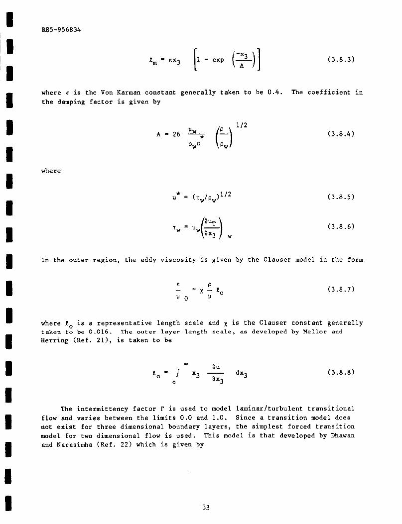
3.8 Turbulence Model

The tu rbu lence model used by Vatsa (Ref. 1 ) i s based on t h e Cebeci and Smith model (Ref . 20) developed f o r two dimensional boundary l a y e r s . This model may be extended t o t h r e e dimensional boundary l a y e r flow by r e p l a c i n g t h e streamwise v e l o c i t y with t h e t o t a l v e l o c i t y . Thus i n t h e i n n e r r eg ion we have

(3.8.1)

where t h e d e r i v a t i v e of t h e t o t a l v e l o c i t y and t h e mixing l eng th are given by

32

1 I I I I 1 I 1 I I 1 1 I I I 1 I 1 I

R85-956834

( 3 . 8 . 3 )

where K is the Von Karman constant generally taken to be 0.4. The coefficient in the damping factor is given by

where

u * = (TW/PW) 112

TW = PW(S) W

( 3 . 8 . 4 )

(3.8.5)

(3.8.6)

In the outer region, the eddy viscosity is given by the Clauser model in the form

P - e - - x - a 0 l J 0 IJ

(3.8.7)

where 11, is a representative length scale and x is the Clauser constant generally taken t o be 0 . 0 1 6 . The outer layer l ength s c a l e , as developed by Mellor and Herring (Ref. 211, is taken to be

Q)

aU

0 3x3 = I x 3 - dx3 (3.8.8)

The intermittency factor r is used to model laminarlturbulent transitional flow and varies between the limits 0.0 and 1.0. Since a transition model does not exist for three dimensional boundary layers, the simplest forced transition model for two dimensional flow is used. This model is that developed by Dhawan and Narasimha (Ref. 22) which is given by

33

R85-9 56834

r = 1 - exp [- 4.6513 (:Ti:TiTl)2] (3.8.9)

where ST1 and ST2 are the specified locations for the beginning and end of transition. Finally we note that three dimensional turbulent boundary layers may have nonisotropic turbulence. Thus the eddy viscosity in the cross flow direction is multiplied by a factor t$ which may take a value as low as 0.40.

3 . 9 Finite Difference Equations

The governing equations described in Section 3.4 are a set of four coupled nonlinear partial differential equations. These equations are reduced by Vatsa (Ref. 2 ) to a set of four coupled nonlinear finite difference equations using the finite difference operators given below.

(3.9.1)

- 53K-l SK+l 3 - 63K-1 53K

34

( 3 . 9 . 4 )

(3.9.5)

I I I I I 1 I 1 1 I I I I I 1 I I 1 1

R85-956834

where Q r e p r e s e n t s a gene ra l s o l u t i o n v e c t o r (F, G , V , H) and t h e i , j, k sub- s c r i p t s r e f e r t o t h e streamwise c l , spanwise c2, and normal E3 l o c a t i o n s r e s p e c t i v e l y . Note t h a t upwind d i f f e r e n c e i s used on t h e c ros s f low convect ive d e r i v a t i v e s depending on t h e s i g n of t h e c ross f low v e l o c i t y so a s t o honor t h e reg ion of dependence c r i t e r i a . When t h e c ross f low v e l o c i t y i s nega t ive , t h e d i f f e r e n c i n g i s e x p l i c i t and t h e r e i s a s t a b i l i t y c r i t e r i a on t h e s t e p s i z e which must be s a t i s i f i e d .

u2 HZ a 2 (3.9.6)

The r e s u l t i n g non l inea r d i f f e r e n c e equat ions a r e quas i - l i nea r i zed t o form a set of l i n e a r ma t r ix equa t ions which a r e solved i n an i t e r a t i v e f a sh ion ( s e e Vatsa , Refs. 1 and 2 ) . The ma t r ix equa t ions are solved by a block s u b s t i t u t i o n a l g o r i - thm descr ibed i n d e t a i l by Vatsa (Ref . 2 ) .

3.10 General ized Surface Coordinates

The computat ional coord ina te s a r e su r face coord ina te s t h a t wrap around the b lade s u r f a c e such t h a t when X 3 = 0.0 , any poin t on t h e s u r f a c e i s a f u n c t i o n of on ly X 1 and X2. bounded by

Furthermore t h e computational domain s h a l l be a r b i t r a r i l y

0.0 < x1 < 1.0 - - (3.10.1)

0.0 < x2 - < - 1 .o

without any l o s s of g e n e r a l i t y and as assumed i n Sec t ion 3.1, t h e coord ina te X 3 s h a l l be normal t o t h e s u r f a c e and hence normal t o both X l and X 2 . The coordi- n a t e s of t h e phys ica l s u r f a c e ( Y1, Y2, Y3> ar'e g e n e r a l l y known on ly i n Car t e s i an c o o r d i n a t e s . Therefore we s h a l l use t h e Car t e s i an coord ina te s as t h e b a s i s f o r t h e t r ans fo rma t ion . (Note s u b s c r i p t s and s u p e r s c r i p t s a r e used t o denote covar- i a n t and c o n t r a v a r i a n t t e n s o r components r e s p e c t i v e l y . ) The purpose of t h i s s e c t i o n is t o f i n d a gene ra l t e n s o r t r ans fo rma t ion from t h e computat ional coord i -

n a t e s (XI t o t h e phys ica l ( C a r t e s i a n ) coord ina te s (Y) f o r an a r b i t r a r y s u r f a c e . It s h a l l be noted a t t h e o u t s e t t h a t t h e Car t e s i an coord ina te s of t h e s u r f a c e a r e g e n e r a l l y not known i n a n a l y t i c a l form but on ly i n numerical form so t h a t a

+ +

35

R85-956834

gene ra l s u r f a c e s p l i n e f i t t i n g a lgo r i thm is requ i r ed t o c o n s t r u c t t h e transforma- t i o n . Thus we are sea rch ing for a t r ans fo rma t ion of t h e form

+ + + Y = Y (XI (3.10.2)

having t h e above p r o p e r t i e s and such t h a t t h e Jacobian

ayi

ax’ J = 1-1 f 0 (3.10.3)

w i t h i n t h e computat ional domain. A nonorthogonal coord ina te system having these p r o p e r t i e s can always be cons t ruc t ed provided t h a t t h e s u r f a c e p r o j e c t s un ique ly t o a p lane s u r f a c e . Thus i f one p r o j e c t s a l l p o i n t s on t h e s u r f a c e on to t h e Y g = 0.0 p lane such t h a t Eq. (3 .10.3) is s a t i s f i e d , t hen uniqueness is assu red . Under

t h e s e cond i t ions , ( s e e F ig . 2 ) , t h e Car t e s i an coord ina te s of t h e s u r f a c e (Y) can be w r i t t e n i n paramet r ic form us ing o n l y t h e computat ional coord ina te s X1, X2). The t r ans fo rma t ion , Eq. (3 .10 .2) , t hen t akes t h e s p e c i a l form

+

Y1 = Y 1 ( x l , x 2 ) ( 3.10.4)

Y2 = Y2 ( x 1 , x2) (3.10.5)

It i s noted t h a t i f t h e t r ans fo rma t ions Eq. (3.10.4) and (3.10.5) are known, then t h e equa t ion of t h e s u r f a c e i n t h e phys ica l c o o r d i n a t e s i s known i n terms of t h e computat ional coord ina te s by d i r e c t s u b s t i t u t i o n v i a Eq. (3.10.6). The t a s k then i s t o de te rmine t h e t r ans fo rma t ions g iven by Eqs. (3.10.4) and (3.10.5). From Fig. 2 , i t i s noted t h a t t h e f o u r boundaries p ro jec t ed onto t h e Y = 0.0 p lane correspond t o

X1 = 0.0 s i d e 1

X2 = 0.0 s i d e 4 (3.10.7)

X1 = 1.0 s i d e 3

X2 = 1.0 s i d e 2

36

R 8 5-9 5 68 34

Thus, as an example, t h e C a r t e s i a n coord ina te s of t h e s i d e 1 boundary can be w r i t t e n i n terms of on ly X 2 as a parameter. on ly a t d e s c r e t e p o i n t s i n t h e form of numerical d a t a , t h e s i d e 1 boundary can parametized with X 2 as a v a r i a b l e us ing t h e fol lowing procedure f o r N boundary p o i n t s .

Since t h e s e boundar ies are known

(3.10.8)

X2 ( I ) = ( I - l ) / (N- l ) I = 1, N

Thus t o each p a i r of p o i n t s Y1( I ) , Y 2 ( I ) t h e r e corresponds a unique X2(1). s imi l a r proceedure is followed on t h e remaining t h r e e s i d e s . With t h e f o u r boundaries w r i t t e n i n paramet r ic form wi th t h e a p p r o p r i a t e X 1 o r X 2 as a v a r i a b l e , any i n t e r i o r po in t i s uniquely c a l c u l a t e d us ing t h e t r a n s f i n i t e mapping of Gordon and Th ie l (Ref. 5 ) .

A

Y i ( x , 1 2 x ) = ( l - x l ) Yi(0, x 2 ) + x 1 Y i ( 1 , x2)

1 2 - (1-X'>(1-X2) Y i (0 , 0)- (1-X )X Y i ( 0 , l ) (3 .10.9)

- x'(1-x2) Y i (1,O) - x1x2 Y i ( l , l )

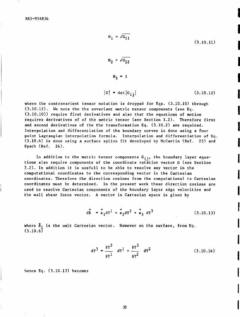
where i = 1,2 . Then g iven any X 1 and X2, t h e Car t e s i an coord ina te s (Y1, Y2 , Y,) are determined un ique ly us ing Eqs. (3.10.9) and E q . (3 .10.6) . The c o v a r i a n t metric t e n s o r components are then determined from

37

(3.10.10)

R8 5-9 5 68 34

(3.10.11)

H3 = 1

I G I = de t lG . - 1 (3.10.12) 1J

where the con t r ava r i en t t enso r n o t a t i o n i s dropped f o r Eqs. (3.10.10) through (3.10.12). W e no te t h e the cova r i an t me t r i c t enso r components ( s e e Eq. (3.10.10)) r e q u i r e f i r s t d e r i v a t i v e s and a l s o t h a t t he equat ions of motion r e q u i r e s d e r i v a t i v e s of of t h e me t r i c t enso r ( s e e Sec t ion 3 .2) . and second d e r i v a t i v e s of t he t h e t ransformat ion Eq. (3 .10.2) a r e r equ i r ed . I n t e r p o l a t i o n and d i f f e r e n t i a t i o n of t h e boundary curves is done us ing a fou r poin t Lagrangian i n t e r p o l a t i o n formula. I n t e r p o l a t i o n and d i f f e r e n t i a t i o n of Eq. (3.10.6) i s done us ing a s u r f a c e s p l i n e f i t developed by McCartin ( R e f . Spath (Ref. 24) .

Therefore f i r s t

23) and

I n a d d i t i o n t o the me t r i c t enso r components G i j , the boundary l a y e r equa- t i o n s a l s o r e q u i r e components of t he coord ina te r o t a t i o n vec to r Q ( s e e Sec t ion 3 .2 ) . I n a d d i t i o n i t i s u s e f u l 1 t o be ab le t o r e s o l v e any vec to r i n t h e computat ional coord ina te s t o the corresponding vec to r i n the C a r t e s i a n coord ina te s . Therefore t h e d i r e c t i o n cos ines from t h e computat ional t o Car t e s i an coord ina te s must be determined. I n t h e p re sen t work these d i r e c t i o n cos ines are used t o r e s o l v e Car t e s i an components of t he boundary l a y e r edge v e l o c i t i e s and t h e w a l l shear fo rce vec to r . A v e c t o r i n Car t e s i an space i s given by

+ 2 + 3 -b -b

dR = eldY1 + e2dY + e3 dY (3.10.13)

where bi i s t h e u n i t Ca r t e s i an v e c t o r . (3.10.6)

However on t h e s u r f a c e , from Eq.

ay3 1 ay3 dY3 = - dY + - dY2

ay3 1 ay3 dY3 = - dY + dY2

~ hence Eq. (3.10.13) becomes

38

( 3 . l o . 14

I I I 1 I I 1 1 I I I 1 1 I I I I I I

R85-956834

(3.10.15)

On t h e s u r f a c e X 3 = 0.0 and

ax ax2 (3.10.16)

ay2 1 ay2

ax1 ax2 dY2 = - dX + - dX2

S u b s t i t u t i n g E q . (3.10.16) i n t o E q . (3.10.151, we have

- + - - ax1 ay2 ax1

-b + ay2 + ay3 ayl dR = [ -b + e2 - el -

ax

- - + dX2 (3 .10.17) ayl ax2 ay2 ax2 ay3 ayl +.; ( + ay2

ax2 + e2 -

' The c o n t r a v a r i a n t components of dR can a l s o be w r i t t e n as

' 2 ' ' + dR = aldX1 + a2dX + a3 ( 0 ) (3.10.18)

+ with a as t h e b a s i s v e c t o r and no t ing t h a t dX3 = 0 on t h e s u r f a c e . comparing terms between E q s . (3 .10 .17) and (3.10.18) we have

Hence by

39

R85-956834

+ e2 - - al - el - ax' ax

(3.10.19)

= el - + e2 - a2 ax2 ax2

The u n i t v e c t o r s then become

+ + + - 1

el ay 1 e2 +

(3.10.20)

+ + + - 1

el ay 1 e 2 ay2 ay3 ay2 I +

where t h e d i s t i n c t i o n between cova r i an t and c o n t r a v a r i a n t v e c t o r s may be dropped. The d i r e c t i o n cos ines are then g iven by

(3.10.21)

Then i f U; i s any v e c t o r i n t h e X i d i r e c t i o n i n t h e computat ional coord ina te s and V. i s any v e c t o r i n t h e Car t e s i an c o o r d i n a t e s , t hen

J

40

I I I I I I I 1 I I I I I I I I I 1 I

I I 1 I I 1 1 I I I 1 I I I I i I I I

R85-956834

- v j - y i j u i

- -1 u j - y i j v i (3.10.22)

3.11 Surface Euler Equat ions

The s o l u t i o n of t he boundary l a y e r equat ions r e q u i r e s s p e c i f i c a t i o n of t h e edge cond i t ions (Ule, U 2 e , HTe, p e , Pe) as shown i n Sec t ion 3.5. These edge cond i t ions can be obta ined d i r e c t l y from experimental d a t a o r t hey can be obtained from s o l u t i o n s of t he Euler equat ions . An a l t e r n a t i v e method is t o so lve t h e su r face Euler equat ions using a known s u r f a c e s t a t i c p re s su re d i s t r i b u t i o n . This method was o u t l i n e d by Cebeci et a l . (Ref. 7 ) f o r a p p l i c a t i o n t o a i r c r a f t wings. Gleyzes and Coust iex (Ref. 8 ) developed a s i m i l a r method f o r incompressible flow over fus i form bodies . This s e c t i o n extends these methods t o o b t a i n a s o l u t i o n of t he compressible su r face Euler equat ions f o r a p p l i c a t i o n t o a r b i t r a r y t h r e e dimensional s u r f a c e such a s t u r b i n e b l ades .

The s u r f a c e E u l e r equat ions can be obtained from the t h r e e dimensional boun- Thus a t dary l a y e r equat ions given i n Sec t ion 3.2 by t ak ing t h e l i m i t a s Xg + m .

t he edge of the boundary and energy equat ions a r e

- l a y e r normal d e r i v a t i v e s vanish and hence t h e momentum w r i t t e n as fol lows:

X1 Momentum

H1 axl L L

(3 .11 .1)

+ C I U l e + C2Uze + c g - - a4 - a CP + a5 - a CP a x l ax2

X2 Momentum

'le au2e '2e au2e 2 2

H 1 a x l H2 ax2 + a6U1e + a7 'le '2e+ a8U2e - - + - -

(3 .11.2)

41

R85-956834

Energy

The c o e f f i c i e n t s i n t h e s e equat ions a r e given by

2 H1H2 1

2lGl p - - - a4 - -

42

(3 .11.3)

I I I 1 I I I 1 I I I I 1 I I I I I I

R 8 5 - 9 5 6 8 3 4

I I

1 a7 - - - [H1H2 [I + ( & ) 2 ]

I G I

1

ax ax, H2 ax2

H12H2 1 a10 = - - -

2 1 G I p

n3 - 2G12 c, - -

JlGl

I I

43

R85-956834

The static pressure has been expressed in terms of the pressure coefficient defined as

(3.11.4)

L

since experimental data is normally given in this form.

Inflow Conditions

The solution of these equations requires specification of the velocity com- ponents Ule and U2e as well as the thermodynamic variables Pe, Te, pe along the inflow boundaries. cient and the freestream or reference stagnation conditions PTm and TTm are known. If the local flow angle can be estimated, then the local edge conditions can be calculated by expanding the flow isentropically from the known stagnation conditions to the local measured static pressure.

In general, only the local surface static pressure coeffi-

A useful relation for this purpose is one between the pressure coefficient and velocity. For incompressible flow this is given by the Bernoulli equation. Since on a rotor the total pressure and total temperature are not constant for the whole flow field, they are assumed constant along a surface of constant radius. function of radius and we have

(The Bernoulli surfaces are cylindrical surfaces). Thus PT and TT are a

-* N

-* P "

2

N

*e P T = P + - ue (3.11.5)

4 4

I I I I I I I I I I I I 1 I I I I I I

I I I I I I I I I I I I I I 1 I I I I

R 8 5-95 6834

where

+ + + + N N + + +

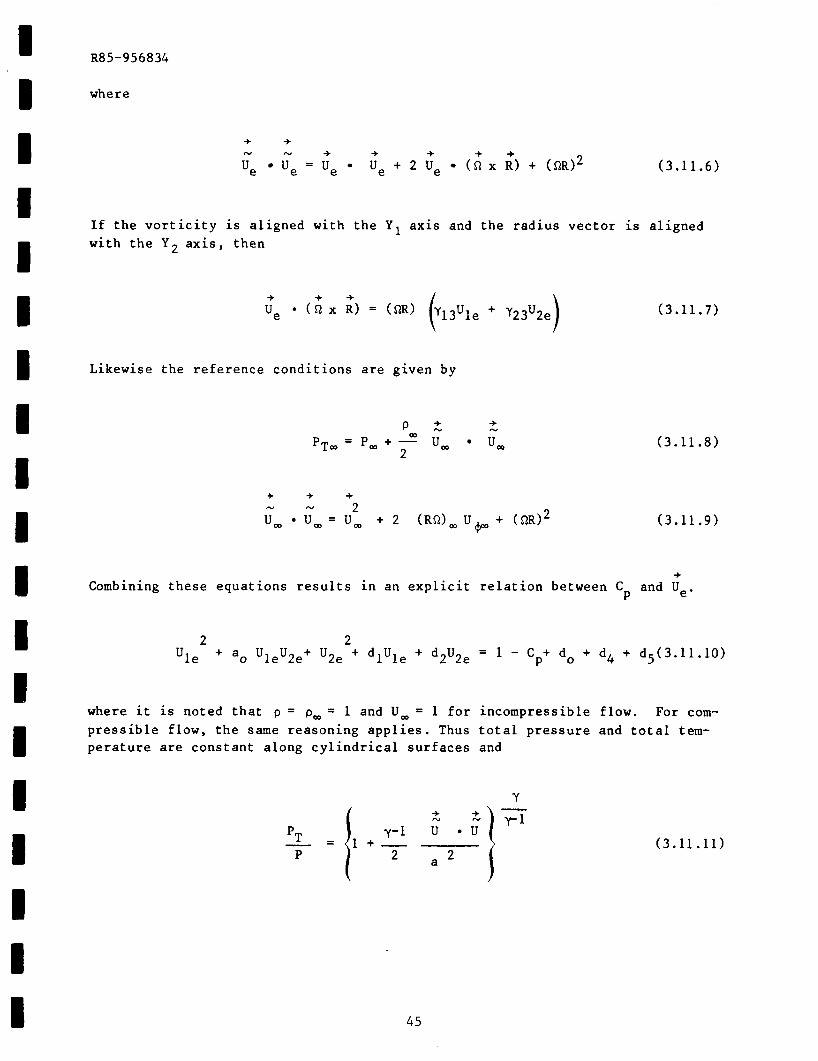
ue ue - - ue ue + 2 Ue ( Q x R) + ( 3 . 1 1 . 6 )

I f t h e v o r t i c i t y i s a l igned with t h e Y1 a x i s and t h e r a d i u s v e c t o r i s a l igned wi th t h e Y2 axis , t hen

Likewise the r e f e r e n c e cond i t ions are given by

p ; t 2

2 m

PT, = P, + - urn Urn

+ + + 2 N N

U, U r n = U, + 2 (RR), U p + (SIR)*

(3.11.7)

(3.11.8)

(3.11.9)

+ Combining t h e s e equa t ions r e s u l t s i n an e x p l i c i t r e l a t i o n between C and Ue . P

where i t i s noted t h a t p = p, = 1 and U, = 1 f o r incompress ib le flow. For com- p r e s s i b l e f low, t h e same reasoning a p p l i e s . Thus t o t a l p r e s s u r e and t o t a l t e m - p e r a t u r e are cons t an t a long c y l i n d r i c a l s u r f a c e s and

pT - P

Y-1 1 + - = I 2

45

2 2 . u * u

2 a i5 (3.11.111

R85-956834

The energy equa t ion can be w r i t t e n as

+ + 2 y-1 -

a T 2 = a + - U - u 2

and combining t h e equa t ions we have,

2 2 = d8 + d9 'le + U2e + 2aoU2e + d l 'le + d2U2e

where t h e c o e f f i c i e n t s a r e g iven by

d3 = 1 - Cp

2 dg = d7aT

1 + - y-l d7 2

46

(3.11.12)

(3.11.13)

I I I I I I I I I I I I I I I I I I I

R85-956834

N N

I A u x i l i a r y Re la t ions

Three a d d i t i o n a l r e l a t i o n s are r equ i r ed t o complete t h e set of equa t ions . These I are t h e eaua t ion of s t a t e

I P = P, 'e

and t h e equat ions f o r t o t a l en tha lpy and r o t h a l p y

2 - Y "Te

HTe - - Te + 7 Y-1

- VB2 Ie - HTe - - 2

S o l u t i o n Algorithm

(3.11.14)

(3.11.15)

(3.11.16)

These equa t ions a re hype rbo l i c equat ions i n which t h e c h a r a c t e r i s t i c s are t h e s t r e a m l i n e s . Therefore t h e s e equat ions have t h e same p r o p e r t i e s as t h e boun- da ry l a y e r equat ions d i scussed i n Sec t ion 3.5 and are so lved by s p e c i f y i n g t h e inf low c o n d i t i o n s on t h e in f low boundary. These in f low c o n d i t i o n s are g iven by (Ule, U 2 e , HTe, Pe) . S ince p r e s s u r e ( i . e . , Cp> i s a known i n p u t , t h e v e l o c i t y components Ule and U2e may be determined by s p e c i f y i n g e i t h e r U2e o r t h e flow angle on t h e inf low p lane and us ing Eq. (3.11.10) o r (3.11.13) t o determine U l e . With t h e v e l o c i t i e s known, t h e tempera ture i s determined from Eq.(3.11.14) and Eq.(3.11.15).

1 I I I

F i n a l l y t h e d e n s i t y i s determined from Eq.(3.11.14).

These equat ions have t h e same p r o p e r t i e s as t h e boundary l a y e r equat ions and t h e f i n i t e d i f f e r e n c e equa t ions are formed i n t h e same manner us ing t h e Eqs. (3 .9 .1) , (3.9.2) and (3 .9 .3) . This r e s u l t s i n a se t of coupled a l g e b r a i c equa- I t i o n s .

47

i R85-956834

bl = a l l + a l

b2 = al lUle,I- l + c1

b3 = a12 + a2

b4 = a12Ule,I ,J-k + '2

u < 0.0

aCP

ax2 + a5 - - acP

axl a13 - a4 -

48

bl = a l l + al

+ c1 al l U l e , 1-1, J b2 = -

b3 = a2

(b4 = a12 ( U l e , I - l , J + l - ' l e , I - l , J ) + '2

I I 1 I I I I I 1 1 I 1 I I 1 1 I 1 1

R85-956834

b5 = a3

bg = a13 + cg

b7 = a6

b8 = -allU2e,I-1,J + '4

bg = all + a7

b10 = 'a12U2e,I,J-l + '5

bll = a8

- b12 - -all + '6

e4 = el + e2

b5 = a3

bg = - a13

b7 = €16

b8 = allU2e, 1-1, J+1-'2e, 1-1 ,J 1 + c5

bg = all + a7

+ c5 - b10 - a12 ('2e,I-l,J+l- '2e,I-l,J

bll = a8

b12 = 'a14

- 'le el -

HIAX1 ,I-1

u2 E

e2 H2AX2, J-1

e4 = el I

where the coefficients on the left side of the page are for U2e > 0.0 and those on the right are for U2e < 0.0. iteratively in a nested loops by successive substitution. for the density. If the flow is incompressible, the density p = 1.0. iteration loop solves f o r the velocity components and rothalpy. known, then Eq. (3.11.17) can be solved for Ule. can be solved for UIZe. the following manner;

Eqs. (3.11.17>,(3.11.18),(3.11.19) are solved The outer loop solves

The inner Assume U2e is

With U !e known, Eq. (3.11.18) Since both equations are quadradlcs, they are solved in

49

R85-956834

4 = (b2 + b3 U2e)2- 4b l (b6 + b4 U2e + bgU2e2) (3.11.20)

= (blo + bg U l e l 2 - 4 b l l (b12 + b8 U l e + b7 Ule2) (3.11.21)

and

(3.11.22)

(3.11.23)

where t h e p o s i t i v e r o o t s are a p p r o p r i a t e . When t h e v e l o c i t y components are known, t h e r o t h a l p y is determined from Eq. (3 .11 .3) , and t h e remaining r o p e r t i e s from Eqs. (3 .11.14) , (3 .11.15) , and (3.11.16) so t h a t t h e d e n s i t y i s updated i n t h e o u t e r i t e r a t i o n loop.

50

I 1 I I 1 I I I 1 I 1 1 I 1 I I 1 I I

R85-956834

4 . 0 RESULTS AND DISCUSSION

4.1 In t roduc to ry Discuss ion

I n t h i s assessment of t h e a p p l i c a b i l i t y of t h r e e dimensional boundary l a y e r t heo ry t o p r e d i c t t h e flow s t r eaml ines and hea t t r a n s f e r i n a gas t u r b i n e passage four reg ions of t h e flow f i e l d are examined. These reg ions a r e t h e t u r b i n e p r e s s u r e s u r f a c e , t h e t u r b i n e endwall s u r f a c e , t h e t u r b i n e s u c t i o n s u r f a c e , and the r o t o r p re s su re s u r f a c e as i n d i c a t e d by t h e shaded a r e a s on F ig . 1. The f i r s t t h r e e cases tes t t h e a n a l y s i s i n a s t a t i o n a r y coord ina te system and t h e f o u r t h i n a r o t a t i n g coord ina te sys tem. Experimental d a t a f o r p r e s s u r e , endwall , and s u c t i o n s u r f a c e s were obta ined by Graz ian i e t . a l . (Ref. 11) i n a l a r g e gas t u r b i n e cascade which s imula ted a t u r b i n e r o t o r . De ta i l ed w a l l s t a t i c p r e s s u r e d i s t r i b u t i o n s , t h r e e component v e l o c i t y t r a v e r s e s , wal l hea t t r a n s f e r , and wal l l i m i t i n g stream l i n e s were p re sen ted . Data f o r t he r o t a t i n g b lade case was obta ined by Dring And J o s l y n (Refs . 1 2 and 13) . This d a t a inc ludes wa l l s t a t i c p r e s s u r e d i s t r i b u t i o n s and w a l l l i m i t i n g s t r e a m l i n e s . I n a d d i t i o n , r a d i a l t r a v e r s e s of t h e t o t a l p r e s s u r e and flow angle i n t h e s t a t i o n a r y r e f e r e n c e frame upstream of the r o t o r were g iven . This d a t a was s u f f i c i e n t t o c a l c u l a t e t h e cases presented i n t h i s s e c t i o n .

I n i t i a l r e s u l t s us ing t h i s t h r e e dimensional boundary l a y e r a n a l y s i s have been presented by Vatsa (Refs . 1 and 2 ) wherein t h e boundary l a y e r edge condi- t i o n s were obta ined d i r e c t l y from t h e v e l o c i t y t r a v e r s e s . I n t h e assessment presented i n t h i s s e c t i o n t h e boundary l a y e r edge cond i t ions w e r e ob ta ined by i n t e g r a t i n g t h e s u r f a c e Eu le r equat ions us ing the measured s t a t i c p r e s s u r e d i s t r i b u t i o n s . The o v e r a l l a n a l y t i c a l procedure, which w a s t h e same f o r a l l ca ses , is shown on t h e flow c h a r t shown on Fig. 3. Sp l ine smoothed C a r t e s i a n coord ina te s of t h e t u r b i n e b lade s u r f a c e a r e used t o c a l c u l a t e a coord ina te system us ing the geometry a n a l y s i s presented i n Sec t ion 3.10. With t h e coord ina te s known, t h e exper imenta l p re s su re d i s t r i b u t i o n was used t o c a l c u l a t e the boundary l a y e r edge cond i t ions u s i n g the sur face E u l e r ana lys i s given i n Sec t ion 3.11. F i n a l l y , t h e t h r e e dimensional boundary l a y e r e q u a t i o n s , given i n Sec t ion 3 .4 , were so lved . The inf low cond i t ions were es t imated us ing the l o c a l s i m i l a r i t y approximation, desc r ibed i n Secton 3 .7 , along a l l in f low p lanes t h a t are not c h a r a c t e r i s t i c s u r f a c e s . For t h e cascade p r e s s u r e s u r f a c e case , t h e p lane of symmetry is a c h a r a c t e r i s t i c s u r f a c e and t h e inf low cond i t ions were e s t ima ted us ing t h e p lane of symmetry a n a l y s i s a l s o desc r ibed i n S e c t i o n 3.7. I n t e g r a l p r o p e r t i e s of t h e boundary l a y e r such as displacement t h i c k n e s s and momentum th i ckness (de f ined f o r a t h r e e dimensional boundary l a y e r ) were c a l c u l a t e d f o r a l l ca ses . These i n t e g r a l p r o p e r t i e s of t h e boundary l a y e r were obta ined from the v e l o c i t y v e c t o r s reso lved i n an i n t r i n s i c coord ina te system def ined by t h e f r e e stream flow d i r e c t i o n and t h e c r o s s flow d i r e c t i o n ( s e e Appendix). I n a d d i t i o n t h e two components of t h e wa l l f r i c t i o n c o e f f i c i e n t (streamwise and c ross f low) , hea t t r a n s f e r (S tan ton number) , and wa l l l i m i t i n g

51

R85-956834

s t r eaml ine skew angles were c a l c u l a t e d . The Stan ton number was c a l c u l a t e d i n two s t e p s . I n the f i r s t s t e p , t h e a d i a b a t i c wa l l t empera ture w a s c a l c u l a t e d by assuming zero h e a t f l u x a t t h e w a l l . I n t h e second s t e p , a cons t an t hea t f l u x equal t o t h a t app l i ed expe r imen ta l ly w a s used, and t h e wal l temperature c a l c u l a t e d . Thus t h e c a l c u l a t i o n procedure used f o r determining t h e S tan ton number w a s t h e same as t h a t used exper imenta l ly i n Ref. 11.

4.2 Turbine Cascade P res su re Surface

The t u r b i n e cascade p r e s s u r e s u r f a c e developes a n e a r l y two dimensional boundary l a y e r s i n c e t h e passage v o r t e x i s near t h e s u c t i o n s u r f a c e as shown on Fig . 1. S ince t h e spanwise s t a t i c p r e s s u r e d i s t r i b u t i u o n i s nea r ly consan t , l i t t l e spanwise flow o r skewing i s expected. For t h i s reason , t h e primary purpose of t h i s t e s t case i s t o demonstrate a c a l c u l a t i o n s t a r t e d along a plane of symme- t r y boundary. The computational domain ex tends from a po in t j u s t down stream from t h e l ead ing edge of t h e t u r b i n e b lade t o a po in t j u s t upstream of t h e t r a i l - ing edge of t h e b lade and spanwise from t h e plane of symmetry t o t h e endwall . The coord ina te s c a l c u l a t e d f o r t h i s case c o n s i s t s of a 40 by 40 g r i d wi th 100 g r i d p o i n t s normal t o t h e s u r f a c e g r i d of which every o t h e r coord ina te l i n e i s p l o t t e d on F i g . 5 . The c a l c u l a t e d boundary layer edge condi t ions are shown on Fig . 6 i n t h e form of v e l o c i t y v e c t o r s p ro jec t ed on t o t h e Y = 0.0 p lane . These v e l o c i t y v e c t o r s show, as expec ted , very l i t t l e spanwise flow a t t h e edge of t h e boundary l a y e r . S ince t h e p re s su re d i s t r i b u t i o n was not a c c u r a t e l y known near t h e l ead ing edge, t h e boundary l a y e r c a l c u l a t i o n was s t a r t e d wi th a f i n i t e bound- a r y l a y e r t h i c k n e s s us ing t h e l o c a l s i m i l a r i t y approximation by spec i fy ing a f i n i t e d i s t a n c e (E,, > 0) f o r t h e v i r t u a l o r i g i n ( s e e Sec t . 3 . 7 ) . The boundary l a y e r was assumed t o be completely t u r b u l e n t th roughout . A p l a t of t h e wa l l l i m i t i n g s t r e a m l i n e s i s shown i n Fig. 7 i n t h e form of t h e w a l l s t ress v e c t o r s p r o j e c t e d on t o t h e Y = 0.0 p lane . Again t h i s v e c t o r p l o t shows ve ry l i t t l e spanwise flow. I n a d d i t i o n , t h e skew angle ( t h e angle between t h e boundary l a y e r edge flow d i r e c t i o n and wa l l s t r e a m l i n e d i r e c t i o n ) i s not more than t e n degrees . These r e s u l t s compare favorably with t h e exper imenta l r e s u l t s f o r flow d i r e c t i o n and flow skewing presented by Graz ian i e t . a l . i n Ref. 11.

3

3

4.3 Turbine Cascade Endwall Sur face

The endwall s u r f a c e boundary l a y e r has a l a r g e c r o s s flow produced by t h e s t r o n g s t a t i c p r e s s u r e g rad ien t from t h e p r e s s u r e s u r f a c e t o t h e s u c t i o n su r face as shown i n F ig . 1. I n a d d i t i o n t h i s boundary l a y e r has a complex p a t t e r n produced by a s e p a r a t i o n and attachment l i n e and a s a d d l e p o i n t . Downstream of t h i s reg ion t h e boundary l a y e r i s r a p i d l y a c c e l e r a t e d and t h e boundary l a y e r growth i s more sys t ema t i c . I n t h i s downstream region it may be p o s s i b l e t o use t h r e e dimensional boundary l a y e r theory . The computational domain and skewed

52

I I 1 I 1 I I I I I E I I 1 I I I I I

R8 5 -9 5 6 8 34

coord ina te system used f o r t h i s ca se i s shown on F ig . 8 . It c o n s i s t s of a 40 by 40 g r i d wi th 100 g r i d p o i n t s normal t o t h e s u r f a c e g r i d which ex tends from a poin t j u s t downstream from t h e saddle po in t t o j u s t upstream of t h e t r a i l i n g edge t o the s u c t i o n s u r f a c e of t he blade passage. The boundary l a y e r edge c o n d i t i o n s were c a l c u l a t e d us ing t h e w a l l s t a t i c p re s su re d i s t r i b u t i o n f o r t h e t h i c k bound- a ry l a y e r case presented by Graz ian i e t . a l . (Ref. 11) . Along t h e inf low bound- aries f o r t h e s u r f a c e Eu le r c a l c u l a t i o n , i t was assumed t h a t t h e boundary l a y e r edge flow was tangent t o t h e X1 coo rd ina te l i n e so t h a t U2e was assumed zero . I n t e g r a t i o n of t h e s u r f a c e E u l e r equat ions showed t h a t f u t h e r downstream smal l nega t ive c r o s s flow v e l o c i t i e s developed i n d i c a t i n g t h a t t h e boundary l a y e r edge flow cu rva tu re was less than the coord ina te cu rva tu re . This r e s u l t was cons is - t e n t wi th t h e v e l o c i t y t r a v e r s e d a t a used by Vatsa (Refs. 1 and 2 ) . Since t h i s s m a l l nega t ive U 2 e v e l o c i t y component produced s t a b i l i t y problems ( s e e S e c t i o n 3 . 9 ) which could not be reso lved even with a much f i n e r g r i d , t h e c a l c u l a t i o n f o r t he edge v e l o c i t y cond i t ions was run assuming t h a t U2e w a s ze ro i n agreement wi th t h e procedure of Vatsa (Ref. 2 ) . A p l o t of t he edge v e l o c i t y v e c t o r s , which a r e tangent t o t h e X 1 c o o r d i n a t e l i n e s , i s shown on Fig . 9 .

The boundary l a y e r c a l c u l a t i o n was s t a r t e d with inf low c o n d i t i o n s obta ined from l o c a l s i m i l a r i t y s o l u t i o n s of t h e boundary l a y e r equa t ions . A comparison of t h e c a l c u l a t e d wa l l shea r v e c t o r s with t h e measured s u r f a c e s t r e a m l i n e s i s shown on F i g . 10. A s seen i n t h i s f i g u r e , t h e flow i n c l i n a t i o n s a r e i n q u a l i t a t i v e agreement with t h e measured d a t a except i n the neighborhood of t he saddle p o i n t . It is a l s o noted t h a t t h e c a l c u l a t i o n presented he re us ing t h e measured wa l l s t a t i c p re s su res t o d e r i v e t h e boundary l a y e r edge cond i t ions shows much b e t t e r agreement f o r t h e p red ic t ed flow angle than t h e c a l c u l a t i o n s of Vatsa (Ref. 2 ) which used measured v e l o c i t i e s f o r t he edge cond i t ions . This r e s u l t i n d i c a t e s t h e d i f f i c u l t y i n de te rmining t h e edge of t h e boundary l a y e r i n a t h r e e dimen- s i o n a l flow f i e l d . Improved r e s u l t s perhaps may be obta ined wi th b e t t e r d e f i n i - t i o n of t h e flow cond i t ions along t h e upstream inf low plane. A comparison of t h e measured and c a l c u l a t e d hea t t r a n s f e r (S tan ton number) d i s t r i b u t i o n s is shown i n F i g . 11 i n t h e form of contour p l o t s . Again q u a l i t a t i v e agreement i s obta ined except i n the reg ion of the sadd le p o i n t . The case presented by Vatsa ( R e f . 1)

i s t h e same as t h a t presented he re except t h a t t h e edge v e l o c i t i e s were d e t e r - mined d i r e c t l y from t h r e e component v e l o c i t y t r a v e r s e s whereas i n t h e p re sen t c a s e t h e edge v e l o c i t i e s were c a l c u l a t e d from t h e wa l l s t a t i c p r e s s u r e d i s t r i b u - t i o n us ing t h e s u r f a c e E u l e r equa t ions . Of i n t e r e s t then i s a comparison of t h e p r e d i c t i o n s of h e a t t r a n s f e r us ing t h e two methods. This i s shown on F ig . 12 i n t h e form of c r o s s e c t i o n p l o t s of S tan ton number vs . spanwise d i s t a n c e a s e v e r a l a x i a l s t a t i o n s . Good q u a l i t a t i v e agreement i s obta ined between t h e two methods where t h e d i f f e r e n c e between t h e resul ts i l l u s t r a t e s the d i f f i c u l t y i n o b t a i n i n g p r e c i s e boundary l a y e r edge cond i t ions from measured d a t a i n a complex t h r e e dimensional flow f i e l d .

5 3

R85-956834

4.4 Turbine Cascade Suc t ion Surf ace

The s u c t i o n s u r f a c e boundary l a y e r of a gas t u r b i n e blade develops s t r o n g t h r e e dimensional e f f e c t s due t o t h e presence of t h e passage vo r t ex which sweeps t h e flow up from the end w a l l s u r f a c e . S ince t h e boundary s t a r t s a t t h e s tagna- t i o n poin t near t h e l ead ing edge of t h e b l ade , t h e l ead ing edge inf low cond i t ions are we l l e s t a b l i s h e d . However t h e flow from t h e end w a l l inflow s u r f a c e produces a s e p a r a t i o n l i n e which d i v i d e s t h e midspan flow from t h e end wal l flow. This inflow i s less w e l l e s t a b l i s h e d . The computational domain and coord ina te system f o r t h i s case is shown on F ig . 13. It c o n s i s t s of a 40 by 40 g r i d with 100 g r i d p o i n t s normal t o t h e su r face g r i d ex tending from j u s t downstream from t h e l ead ing edge of t h e b lade t o j u s t upstream of t h e t r a i l i n g edge of t h e b lade and from t h e end wa l l t o t h e mid p lane or plane of symmetry. The boundary l a y e r edge condi- t i o n s were c a l c u l a t e d assuming ze ro c r o s s flow v e l o c i t i e s a t t h e l ead ing edge inflow p lane . Along t h e endwall in f low p lane , t h e flow angle and hence c r o s s flow U2e v e l o c i t y was e s t ima ted from t h e measured s u r f a c e s t r eaml ines given by Graz ian i et a l . (Ref. 11 ) . A p l o t of t h e c a l c u l a t e d edge v e l o c i t y v e c t o r s i s shown on F ig . 14. S ince t h e cascade s u r f a c e i s a developable s u r f a c e , t h e v e c t o r p l o t i s shown us ing a r c l eng th as c o o r d i n a t e s . This vec to r p l o t c l e a r l y shows t h e e f f e c t of t h e passage v o r t e x on t h e flow at t h e boundary l a y e r edge. S ince t h e su r face Eu le r equa t ions a r e hype rbo l i c equa t ions w i t h s t r eaml ines as t h e c h a r a c t e r i s t i c l i n e s , t h i s case i l l u s t r a t e s d i f f i c u l t i e s which may be encountered as t h e flow approaches t h e plane of symmetry. The o v e r a l l flow d i r e c t i o n i s from the endwall t o t h e p lane of symmetry. Therefore t h e flow along t h e plane of symmetry i s a r e s u l t of t h e c a l c u l a t i o n not an input boundary o r inflow cond i t ion . Along t h i s p lane of symmetry t h e c r o s s flow v e l o c i t y i s ze ro . Hence t h e s t a t i c p re s su re m u s t be such a s t o reduce t h e c r o s s flow v e l o c i t y t o ze ro a t t h e p lane of symmetry. I n gene ra l without s u f f i c i e n t d a t a t h i s may be d i f f i c u l t t o achieve as was found i n t h e p re sen t ca se near t h e b lade t r a i l i n g edge.

The t h r e e dimensional boundary layer equa t ions were solved us ing l o c a l s i m i l a r i t y inf low c o n d i t i o n s as desc r ibed i n Sec t ion 3.7 and t h e l o c a l c a l c u l a t e d edge c o n d i t i o n s . S ince t h i s is a t r a n s i t i o n boundary l a y e r , t h e begin ing and end of t r a n s i t i o n must be e s t ima ted because t h e p re sen t a n a l y s i s l acks a t r a n s i t i o n model f o r t h r e e dimensional boundary l a y e r s . The begin ing and end of t r a n s i t i o n were obta ined by c a l c u l a t i n g t h e quasi-two dimensional flow along t h e p lane of symmetry us ing t h e i n t e r m i t t a n c y func t ion of Dhawan and Narashima (Ref , 22) and comparing t h e r e s u l t s wi th t h e exper imenta l d a t a f o r hea t t r a n s f e r . t r a n s i t i o n p o i n t s were then he ld cons t an t ac ross t h e span of t h e b l ade . A com- pa r i son of t h e c a l c u l a t e d w a l l shea r v e c t o r s wi th t h e measured wa l l l i m i t i n g s t r eaml ines i s shown on Fig . 15. The flow d i r e c t i o n at t h e w a l l i s seen t o be c a l c u l a t e d q u i t e w e l l and t h e s e p a r a t i o n l i n e s e p a r a t i o n l i n e d i v i d i n g t h e lead- ing edge flow from the end wa l l flow i s a l s o p r e d i c t e d q u i t e w e l l . A comparison of t h e measured and c a l c u l a t e d S tan ton number d i s t r i b u t i o n s i s shown on Fig . 16.

These

54

R85-9 5 6834

Again encouraging agreement i s obta ined both as t o magnitude and o v e r a l l p a t t e r n . The c a l c u l a t i o n , however appears t o underpredic t t he peak hea t t r a n s f e r which occurs nea r t h e endwall i n f low p lane . ve r sus spanwise d i s t a n c e a t d i f f e r e n t a x i a l s t a t i o n s are shown on Fig . 17. These p l o t s show t h a t t h e average l e v e l of hea t t r a n s f e r a c r o s s t h e span i s p red ic t ed reasonably w e l l , but t h a t t h e high and low reg ions are unde rp red ic t ed . Calcu- l a t e d and measured hea t t r a n s f e r along t h e midplane of t h e b l ade is shown on F ig . 18. This f i g u r e a l s o shows p r e d i c t i o n s made from a two dimensional c a l c u l a t i o n us ing t h e p re sen t t h r e e dimensional boundary l a y e r a n a l y s i s and a l s o p r e d i c t i o n s made by Sharma (Ref. 25). These comparisons show t h a t although t h e flow i s q u a s i two dimensional along t h e plane of symmetry ( i . e . U2e = 0.01, t h e h e a t t r a n s f e r is not p red ic t ed a c c u r a t e l y . Sharma (Ref. 251, wi th a quas i 3-D c a l c u l a t i o n , showed t h a t t h i s d i f f e r e n c e can be accounted f o r by t h e s t r e a m l i n e convergence of t h e flow toward t h e p lane of symmetry. Thus it may be expected t h a t t h e d i f f e r - ence between t h e c a l c u l a t e d 3-D hea t t r a n s f e r and t h e measured h e a t t r a n s f e r can i n l a r g e p a r t be accounted f o r by e r r o r s i n t h e p r e d i c t i o n of s t r e a m l i n e conver- gence. Vatsa (Ref. 1 ) ob ta ined b e t t e r p r e d i c t i o n s of t h e h e a t t r a n s f e r along t h e midplane us ing measured v e l o c i t i e s f o r t h e edge cond i t ions . S ince no p r e s s u r e d i s t r i b u t i o n d a t a w a s a v a i l a b l e from t h e quar te r -p lane t o t h e midplane f o r t h i s case , t he s t r e a m l i n e convergence of t he flow towards t h e midplane could not be e s t ima ted by t h e s u r f a c e E u l e r a n a l y s i s as a c c u r a t e l y as o therwise might be p o s s i b l e .

Crossec t ion p l o t s of t h e S tan ton number

The t h r e e dimensional boundary l a y e r a n a l y s i s a l s o c a l c u l a t e s t h e wa l l f r i c - t i o n c o e f f i c i e n t s and i n t e g r a l parameters such as displacement and momentum th i ckness . S ince a nonorthogonal coord ina te system may be r a t h e r a r b i t r a r y and not r e f l e c t t h e flow p r o p e r t i e s , t h e s e parameters are c a l c u l a t e d i n a l o c a l l y i n t r i n s i c coord ina te system ( s e e Appendix). This l o c a l l y i n t r i n s i c c o o r d i n a t e system i s r e fe renced t o t h e boundary l a y e r edge flow d i r e c t i o n and an or thogonal c r o s s flow flow d i r e c t i o n . A l l v e l o c i t i e s and shear stresses a r e l o c a l l y reso lved t o t h i s coord ina te system. Thus two displacement th i cknesses are de f ined . One r e p r e s e n t s t he v e l o c i t y de fec t i n t h e streamwise d i r e c t i o n and t h e o t h e r t h e v e l o c i t y d e f e c t i n the cross flow d i r e c t i o n . L i k e w i s e the w a l l f r i c t i o n coe f f i - c i e n t s r e p r e s e n t s t h e wall shea r i n t h e streamwise and c r o s s flow d i r e c t i o n . Contour p l o t s of t h e streamwise component of w a l l f r i c t i o n c o e f f i c i e n t and displacement th i ckness a r e shown on Figs . 19 and 20.

4.5 Turbine Rotor P r e s s u r e Sur face

The flow over the r o t o r p re s su re s u r f a c e i s s t r o n g l y in f luenced by t h e r e l a - t i v e v o r t i c i t y genera ted by r o t a t i o n of coord ina te s . Thus t h e boundary l a y e r flow i s d r i v e n by two app l i ed f o r c e s ; t h e p re s su re g r a d i e n t , and t h e C o r i o l i s f o r c e . Because of r o t a t i o n r o t a t i o n , t h e p r e s s u r e s u r f a c e s e e s a s t r o n g r a d i a l p re s su re g rad ien t which tends t o d r i v e t h e flow r a d i a l l y inward. The C o r i o l i s

55

R85-956834

fo rce may tend t o d r i v e t h e flow r a d i a l l y inward or outward depending on t h e s i g n of t h e b lade r o t a t i o n vec to r normal t o t h e s u r f a c e C13. f o r c e s tends t o d r i v e t h e flow r a d i a l l y outward nea r t h e l ead ing edge and a x i a l l y near t h e t r a i l i n g edge. The computational domain and coord ina te g r i d f o r t h i s problem i s shown on Fig . 21. It c o n s i s t s of a 40 by 40 g r i d with 100 g r i d p o i n t s normal t o t h e s u r f a c e g r i d ex tending from j u s t downstream from t h e l ead ing edge s t a g n a t i o n l i n e t o j u s t upstream of t h e t r a i l i n g edge and from t h e r o t o r hub t o t h e r o t o r t i p . The boundary l a y e r edge v e l o c i t y v e c t o r s c a l c u l a t e d from t h e sur - f a c e Eu le r equa t ions a r e shown on F ig . 22. It was found t h a t no s o l u t i o n of t h e s u r f a c e Eu le r equat ions e x i s t a long t h e l ead ing edge inf low boundary f o r t h e c ross f low v e l o c i t y U2e = 0.0. Therefore on both t h e l ead ing edge and hub inf low boundar ies , t h e c ross f low v e l o c i t y was es t imated from t h e su r face s t r e a m l i n e s given by Dring and Jos lyn (Refs . 12 and 13) . behavior of t h e s u c t i o n s u r f a c e flow observed by Dring and Jos lyn .

The ba lance of t hese

The edge v e l o c i t i e s show t h e

The boundary l a y e r equa t ions were s t a r t e d wi th l o c a l s i m i l a r i t y inf low c o n d i t i o n s . A comparison of t h e c a l c u l a t e d wall stress v e c t o r s w i th t h e wa l l s t r eaml ines obta ined us ing t h e ammonia-ozalid process i s shown on F ig . 23. The c a l c u l a t e d v e c t o r s c l e a r l y show t h e gene ra l o v e r a l l flow p a t t e r n q u i t e we l l . Calcu la ted flow angles a re compared wi th t h e flow angles measured from t h e o z a l i d paper on Fig. 24. Two curves are shown. The first curve (solid line) is the c a l c u l a t e d flow angle a t each po in t along t h e c a l c u l a t e d s t r eaml ine . The second curve ( d o t t e d l i n e ) i s the c a l c u l a t e d flow angle along t h e midplane. A compari- son of t h e edge v e l o c i t y v e c t o r s with t h e wal l v e c t o r s i n d i c a t e s t h a t t he flow skewing i s up t o about t e n deg rees . These f i g u r e s c l e a r l y show t h a t t h e flow s t r eaml ines a r e p red ic t ed f a i r l y a c c u r a t e l y and t h a t two dimensional boundary l a y e r theory app l i ed i n a s t r i p f a sh ion would not be adequate t o c a l c u l a t e t h e hea t t r a n s f e r on t h e t u r b i n e b l ade . Ca lcu la t ed S tan ton number d i s t r i b u t i o n s f o r a f u l l y t u r b u l e n t boundary l a y e r are shown on F i g . 25. Th i s shows h ighe r hea t t r a n s f e r rates near t h e hub and t r a i l i n g edge of t h e r o t o r b lade .

56

I I 1 I 1 1 ! I 1 I 1 I 1 1 I 1 I I I

I 1

R85-956834

5.0 CONCLUDING REMARKS

1 1 I

I I 1

An assessment has been made of t h e a p p l i c a b i l i t y of a t h r e e dimensional boundary l a y e r a n a l y s i s f o r t h e c a l c u l a t i o n of hea t t r a n s f e r , t o t a l p r e s s u r e l o s s , and s t r e a m l i n e flow p a t t e r n s on t h e s u r f a c e s of both s t a t i o n a r y and r o t a t i n g t u r b i n e passages . On t h e p re s su re and s u c t i o n s u r f a c e of a t u r b i n e cas- cade, t h e 3-D boundary layer a n a l y s i s along with the coord ina te gene ra to r and s u r f a c e Eu le r a n a l y s i s produce p r e d i c t i o n s of hea t t r a n s f e r and s u r f a c e stream- l i n e pat t e r n s which a r e i n reasonably good agreement wi th a v a i l a b l e exper imenta l d a t a . Experimental d a t a f o r wa l l f r i c t i o n c o e f f i c i e n t was not a v a i l b l e t o e v a l u a t e the p r e d i c t i o n of l o s s ; however, because of t h e c l o s e r e l a t i o n between wa l l f r i c t i o n and h e a t t r a n s f e r one may a l s o expect good p r e d i c t i o n s of l o s s . Assessment of t h e 3-D boundary l a y e r a n a l y s i s f o r t h e p r e d i c t i o n s of t h e flow on a t u r b i n e endwall i s complicated by t h e u n c e r t a i n t y i n t h e inf low cond i t ions downstream from the s e p a r a t i o n and attachment l i n e s . However t h e r e s u l t s ob ta ined i n t h i s s tudy a r e very encouraging a s they i n d i c a t e t h a t t h e 3-D bound- a ry l a y e r a n a l y s i s i s a p p l i c a b l e t o t h e endwall s u r f a c e as we l l . On t h e p r e s s u r e s u r f a c e of a r o t a t i n g t u r b i n e b l ade , p r e d i c t i o n of t h e flow s t r e a m l i n e s and flow skewing agree reasonably wel l with t h e a v a i l a b l e d a t a . Evalua t ion of t h e analy- s i s f o r t h e p r e d i c t i o n of h e a t t r a n s f e r and l o s s on a r o t a t i n g t u r b i n e b lade must await the c o l l e c t i o n of exper imenta l d a t a .

The r e s u l t s ob ta ined i n t h i s i n v e s t i g a t i o n r e i n f o r c e e a r l i e r conclus ions t h a t two dimensional boundary l a y e r theory appl ied i n a s t r i p f a sh ion can not p r e d i c t hea t t r a n s f e r and l o s s because of t he s t r o n g t h r e e dimensional flow e f f e c t s on a t u r b i n e b l ade . On t h e s u c t i o n s u r f a c e of a b l ade , t h e s e t h r e e dimensional e f f e c t s a r e produced by t h e passage v o r t e x and on the p r e s s u r e s u r f a c e of a r o t a t i n g b lade t h e s e e f f e c t s are produced by t h e r a d i a l p r e s s u r e g rad ien t and C o r i o l i s f o r c e . I n view of t h e c u r r e n t s ta te of Navier-Stokes analy- s i s , t h r e e dimensional boundary l a y e r theory could provide a u s e f u l t o o l f o r l o c a l enhancement of of t h e flow f i e l d f o r t he p r e d i c t i o n of hea t t r a n s f e r , l o s s , and flow s t r e a m l i n e p a t t e r n on t u r b i n e b lade s u r f a c e s . The resu l t s of t h i s s t u d y s t r o n g l y i n d i c a t e t h a t the l o c a l d e t a i l s of t h e flow f i e l d on t h e t u r b i n e b l ade s u r f a c e can be a c c u r a t e l y c a l c u l a t e d us ing a two s t e p procedure. F i r s t t h e over- a l l flow f i e l d can be c a l c u l a t e d on a coa r se g r i d us ing a Navier-Stokes o r parabol ized Navier-Stokes a n a l y s i s . Second t h e t h r e e dimensional boundary l a y e r a n a l y s i s can be used f o r l o c a l enhancement t o provide d e t a i l s of t h e flow f i e l d on a much f i n e r g r i d .

57

R85-956834

6 .0 ACKNOWLEDGEMENT

The au tho r wishes t o acknowledge t h e c o n t r i b u t i o n s of D r . V. Vatsa of NASA Langley Research Cen te r and D r . J. Carter and B. Cap l in of UTRC. I n a d d i t i o n , t h e au tho r wishes t o n o t e t h a t development of computer codes t o p l o t r e s u l t s of t h e boundary l a y e r a n a l y s i s were t h e r e s u l t of independent r e s e a r c h a c t i v i t i e s a t UTRC .

58

I I 1 I I I 1 I 1 1 1 I 1 I I 1 1 I 1

R8 5 -9 5 6 8 34

7 .O REFERENCES

1.

2 .

3.

4 .

5 .

6 .

7 .

8 .

9 .

10.

11.

12 .

Vatsa, V . N . : A Three-Dimensional Boundary-Layer Analys is Inc luding Heat Trans fe r and Blade Ro ta t ion E f f e c t s , Paper p re sen ted a t t h e Thi rd Symposium on Numerical and Phys ica l Aspects of Aerodynamic Flows, Long Beach C a l i f o r n i a , January 1985.

Vatsa, V . N . : A Three Dimensional Boundary Layer Analys is f o r Turbomachinery App l i ca t ions , UTRC Report No. 84-44, 1984.

Howarth, L. : The Boundary Layer i n Three-dimensional Flow Along a General Three Dimensional Su r face , P h i l . Mag. S e r i e s 7 , Vol. 42 p 239 - 243 1951.

Squ i re , L. C . : The Three-Dimensional Boundary Layer Equat ions and Some Power S e r i e s S o l u t i o n s , ARC Tech. Rpt. R6M 3006 1957.

Gordon, J . W . and T h i e l , L . C . : T r a n s f i n i t e Mappings and The i r App l i ca t ion t o Grid Genera t ion , Numerical Grid Genera t ion , F . Thompson Ed., E l s e v i e r Sc ience Pub l i sh ing Co. I n c . 1982.

Mager, A , : Three Dimensional Laminar Boundary Layers , High Speed Aerodyna- mics and J e t P ropu l s ion , Ed. by F . K . Moore, Vol. I V , P r i n c t o n U n i v e r s i t y P r e s s , P r i n c t o n New J e r s y 1964 p. 286 - 394.

Cebeci, T . , K . Kaups, and J . A. Ramsey: A General Method For C a l c u l a t i n g Three Dimensional Compressible Laminar and Turbulent Boundary Layers on A r b i t r a r y Wings, NASA CR-2777, January 1977.

Gleyzes, C . , and J . Cousteix: Ca lcu la t ion of S t reaml ines from Wall P r e s s u r e s on a Fusiform Body, Rech. Aerosp. 1984-3.

B l o t t n e r , F. G. : F i n i t e d i f f e r e n c e Method of s o l u t i o n of t h e Boundary Layer Equat ions , AIAA J o u r n a l , Vol. 18, p . 193-205 February 1970.

Werle, M. J . and J . M . Verdon: V i s c i d / i n v i s c i d I n t e r a c t i o n Analys is f o r Symmetric T r a i l i n g Edges, UTRC Report R79-914493-5 January 1980.

G r a z i a n i , R. A . , B la i r , M . F . , Tay lo r , J . R . and Mayle, R . D . : An Experi- mental Study of Endwall and A i r f o i l Su r face Heat T r a n s f e r i n a Large Sca le Turbine Blade Cascade, Trans . ASME, J . of Eng. f o r Power, V o l . 102, No. 2 , A p r i l 1980, p. 257-267.

Dring, R. P . , and J o s l y n , H. D . : Measurements of Turbine Rotor Blade Flows, Trans. ASME J . of Eng. f o r Power, Vol 103, No. 2 , A p r i l 1981, p. 400-405.

59

13.

14.

15.

16.

17.

18.

19.

20.

21.

22.

23.

24.

25.

26.

Dring, R. P. and H. D. Joslyn: The Relative Eddy in Axial Turbine Rotor Passages, ASME paper 83-GT-22, 1983.

Warsi, 2 . U. A . : Tensor and Differential Geometry Applied to Analytic and Numerical Coordinate Generation, Mississippi State University Report MSSU- EIRS-81-1, December 1980.

Bradshaw, P.: Effects of Streamline Curvature on Turbulent Flow, AGARDograph No. 169, August 1973.

Blottner, F. G.: Computational Techniques for Boundary Layers AGARD Lecture Series 73, presented at VKI, February 1975.

Vatsa, V. N. and Davis, R. T.: The Use of Levy-Lees Variables in 3-D Boundary Layer Flows. NASA CR-112315, January, 1973.

Wang, K. C.: On the Determination of the Zones of Influence and Dependence fo r the Three dimensional Boundary Layer Equations, J. Fluid Mech. Vol. 8 , 1971, p. 397 - 404. Blottner, F. G. and Ellis, M. A . : Finite Difference Solution of the Incom- pressible Three - Dimensional Boundary Layer Equations for a Blunt Body, Int. J. of Computers and Fuids Vol. 1, 1973 p. 133 - 158.

Cebeci, T. and Smith, A. M. 0.; Analysis of Turbulent Boundary Layers, Academic Press, New York, 1974.

Mellor, G. L. and Herring, H. J.: Simple Eddy Viscosity Relations for Three Dimensional Turbulent Boundary Layers, AIAA J., Vol. 15 No. 6, 1977, p 886 - 887.

Dhawan, S . and Narasimha, R.: Some Properties of Boundary Layer Flow During Transition from Laminar to turbulent Motion, J. of Fluid Mechanics, Vol 3, 1958, p. 418-436.

McCartin, B. J. : Theory,Computation,and Application of Exponential Splines, Courant Mathematics and Computing Laboritories,October 1981.

Spath, H. : Spline Algorithms f o r Curves and Surfaces, Utilitas Mathematica Publishing Co. Inc., Winnipeg, 1974

Sharma, 0. P., and Graziani, R. A,: Influence of Endwall Flow on Airfoil Suction Surface Midheight Boundary Layer Development in a Turbine Cascade, Trans. ASME J. of Eng. for Power, Vol 105 January 1983, p 147-155

Anderson, 0. L. and B. Caplin: User's Manual f o r Three Dimensional Boundary Layer Code, UTRC Report R85-956834-1, March 1985.

60

R85-956834

8.0 LIST OF SYMBOLS

‘n

Kn

cpJ cv

Cf

CP

ei +

F

gijJ Gij

G

h J

h J H

hTJ HT

H

i J I

k

11

L

M

+ “i

P J p

Coefficients of boundary edge equations

Coefficients of boundary layer equations

Specific heats

Wall friction coefficient

Pressure coefficient

Unit vectors Cartesian coordinates

X2 velocity ratio

Covarient metric tensor components

X velocity ratio

Metric scale coefficients

Static enthalpy

Total enthalpy

Total enthalpy ratio

Rot ha lpy

Thermal conductivity

Reference length

Levy - Lees parameter

Mach number

Unit vectors surface coordinates

Static pressure

61

Tota l p re s su re

P r a n d t l number l amina r / tu rbu len t

Levy - Lees l eng th s c a l e parameter

Heat f l u x

Radius

Reynolds number

Gas cons t an t

Arc l eng th d i s t a n c e

S tan ton number

S t a t i c temperature

Veloc i ty components s u r f a c e coor .

Axial v e l o c i t y

Radia l v e l o c i t y

Tangen t i a l v e l o c i t y

X2 r e fe rence v e l o c i t y

Ve loc i ty components Car t e s i an coor .

X j reduced v e l o c i t y

Rotor v e l o c i t y

Surface coord ina te s

C a r t e s i a n coord ina te s

R e l a t i v e i n l e t flow angle

Ra t io of sDec i f i c h e a t s

'ie Or U2e

6 2

R85-9 5 6834

Yi j

-1 Yi j

6

E

- ‘ref

8

8

U

pref

si

PY P

‘I

Direction cosine tensor components

Inverse tensor components

Displacement thickness

Eddy viscosity

Viscosity ratio turbulentllaminar

Reference viscosity ratio

Momentum thickness

Static temperature ratio

Molecular viscosity

Reference molecular viscosity p(tref)

Levy - Lees transformed coordinates

Density ( P I P , )

Time

Stress components

Rotor speed

Subscripts

C Cross flow direction

e Edge conditions

h Hub

L rotor inlet conditions

S Streamwise direction

t Tip

T Total or stagnation conditions

m Free stream or reference conditions

63

( t It ref 1

R85-956834

Superscripts

N Absolute rotor reference frame Tensor Not at ion

i y j y k Subscripts covarient tensor components

iyj,k Superscripts contravarient tensor components

6 4

I I 1 I 1 1 1 I 1 1 1 1 I I I i I 1 1

HORSESHOE VORTEX 7

CROSS

a AREAS OF APPLICATION FOR 3-DBL

*SUCTION SURFACE *ENDWALL REGION *PRESSURE SURFACE

Fig. 1 Flow in a Turbine Passage

84-1 2-33-7

65

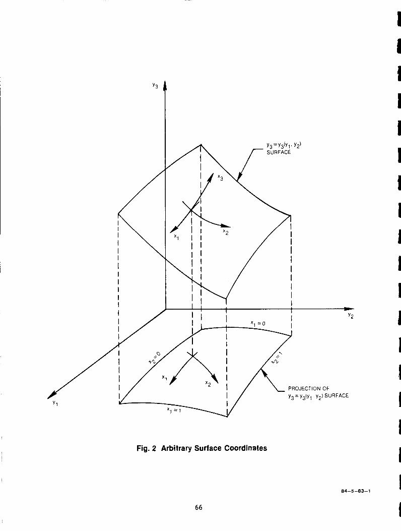
y3 1

Fig. 2 Arbitrary Surface Coordinates

84-5-83-1

66

I 1 1 I 1 I 1 I I 1 1 I I 4 I I I I 1

BLADE DESCRIPTION KNOWN Y1, Y2. Y3 CARTESIAN COORDINATES

FLOW CONDITIONS KNOWN WALL PRESSURE Cp (Y1, Y2. Yg)

SURFACE EULER GEOMETRY ANALYSIS

I 7- EDGE VELOCITIES \

Y, Y 2 3 Y CARTESIAN r O n R n l N A T F S 7 I \ g,, h, ME1 nib vn I n

KNOWN AS A FUNCTION OF X, X2 X3 SURFACE COORDINATES

I U1 U2 KNOWN AS A FUNCTION OF X, X2 X3 SURFACE COORDINATES

3-D BOUNDARY LAYER ANALYSIS

BOUNDARY LAYER PARAMETERS 6'. 8, Cf. S KNOWN

Y,, Y2. Y3 CARTESIAN COORDINATES AS A FUN~TION OF

Fig. 3 Flow Chart of Geometry, Surface Euler and 3-D Boundary Layer Analysis

84-5-103-1

57

ZONE OF

Fig. 4 Zone of Influence and Zone of Dependance for Three Dimensional Boundary Layers

68

I I 1 I 1 I 1 I 1 I I I I I 1 I I 1

85- 1-87- 12

TRAILING EDGE

PLANE OF

E :ND WALL

Fig. 5 Coordinate System Calculated for Cascade Pressure Surface

04-5-04-1

69

0.66E

0.55:

0.441

Y2 0.333

0.222

0.1 11

0

PLANE OF SYMMETRY

I 1 I

' END WALL

0.1 71 0.306 0.441 0.576

Y l

0.71 1 0.846 0.981

Fig. 6 Boundary Layer Edge Velocity Vectors Projected on Y3 Plane Calculated from Experimental Static Pressure Distribution for the Cascade Pressure Surface

84-5-84-2

70

1 1 I 1 I 1 1 I I 1 1

0.666

0.555

0.444

y 2 0.332

0.222

0.1 11

0

PLANE OF SYMMETRY c = - - - - = - - - - -

- L - - T

I- 5

END WALL

0.1 71 0.306 0.441 0.576

Y1

0.71 1 0.846 0.981

Fig. 7 Boundary Layer Wall Shear Vectors Projected on Y3 Plane Calculated with the 3-Dimensional Boundary Layer Analysis for the Cascade Pressure Surface

84-5-84-3

71

y2 f :SSUF I E i SIDE

Fig. 8 Coordinate System for Cascade Endwall Surface

I 1 I I 1 1 1 I I 1 I I I 1 1 I I I

85-1-87-11

72

Fig.

V

Boundary Layer Edge Velocity Vectors Calculated from Experimental Surface Pressure Distributions for Cascade Endwall Surface

85-1-87-2

73

a

4 w >

I- W J z

0 C .- I

.c 0

L

0 7

I 1 1 I 1 1 1 I I I I I I I I 1 I I 1

83-12-69-1

74

I

\

I

qw

P,~,Cp(ta-~,) st =

1 5 in INLET BOUNDARY LAYER

MEASURED

I

CALCULATED

Fig. 11 Comparison of Measured and Calculated Stanton Number Distributions for End Wall Surface

85-1 -87-1

75

qw

p, u c (t - tw) st =

w P a 0 EXP DATA(REF 11)

CALC (REF 1) PRESENTCALC

- -- -

X =0.8 1

0.0 t

cij' 0.003

0 z

0.0 1 z

O I

- 0.2

0.003 - 0, do- -

"0 0.2 0.4 0.6 0.8 1 .o

GAPWISE DISTANCE X2

Fig. 12 Comparison of Stanton Number Distributions on Endwall Surface

I 1 I I I 1 1 I 1 1 I I I

- 1 I I

85-1-87-3

76

LEAC

Ir y2

IETRY

\ TRAILING EDGE

Fig. 13 Coordinate System Calculated for Cascade Suction Surface

04-7-33-1

77

Sl

Fig. 14 Boundary Layer Edge Velocity Vectors Calculated from Experimental Surface Pressure Distribution for Cascade Suction Surface

78

I 1 1 I 1 I 1 I I I I I I I I 1 I I 1

84-1 2-33-1

1 1 1

MEASURED

MID r L " t

N SEPARATION LINE v)

HUB

MID

0 Sl

CALCULATED

PLAN E

cv v)

HUB 0

Sl 1.47

1.6

Fig. 15 Measured and Calculated Wall Limiting Streamline on Cascade Suction Surface

84-12-33-4

79

MID PLAN E

CJ cn

HUB

MID

MEASURED

0 0 2 0 4 0 6 0 8 1 0 1 2 1 4 1 6

S1

CALCULATED

N 0.22 - cn

0 0 26 0 51 0 7 5 0.99 1 2 3 1 4 7

S1

Fig. 16 Measured and Calculated Stanton Number on Cascade Suction Surface

80

I 1 1 I I I I I I I I 1 I I I I I 1 1

84-12-33-5

S = 1 . 4 4 0 1 0 I

z 0.0 e Z a I- o 0.003

o-

0 72 -

0 u w

O O 0 -

MID SPAN

0.0

0.003

I 0 z

-

0.36 0 --- O O v

I 1 I 0 0.2 0.4 0.6 0.8 1 .o 0.0 L

SPANWISE DISTANCE S2

Fig. 17 Comparison of Stanton Number Distributions on Cascade Suction Surface

85-1 -87-10

81

m-

0.004- st = 9 ,

I Peu,Cp('a -'w'

I #

I 0.003 - I

\ - - - ===- --= - -- ---- -- 0- -

0- - -- - 0- 0 0

0.001 -

0 EXP DATA (REF 11) CALC 2D

CALC 3 0 --- CALC. 2D (REF 25) ---- - - - CALC QUASI 3D (REF 25)

S1

Fig. 18 Calculated and Measured Stanton Number on Mid Plane of Cascade Suction Surface

I I I I I I I I I 1 I I I I I I I I I

84-12-33-2

a2

I 1 8 I I I I I I I I I I I I I I I I

MID PLANE

0.44 -

0.02 0.26 0.51 0.75 0.99 1.23 1.47 L.E. T.E.

S1

Fig. 19 Streamwise Component of Wall Friction Coefficient on Cascade Suction Surface

85- 1-87-4

83

0.02 0.26 L.E.

MID PLANE

0.44 -

mN 0.22-

Fig. 20 Streamwise Component of Displacement Thickness on Cascade Suction Surface

84

~

I I I I I I I I I 1 I I I I I I 1

85-1-87-5 I I

0.51 0.99 1.23 1.47 T.E.

S1

Fig. 21 Coordinate System Calculated for Turbine Rotor Pressure Surface

85-1 -87-6

85

TIP

N a

~~

A . . . . . . . _ . . . . . . . . . . . . . . . _ . . ~ . . . . . _

i L.E. T.E.

Sl

Fig. 22 Boundary Layer Edge Velocity Vectors Calculated from the Experimental Pressure Distribution for the Pressure Surface of a Rotating Turbine Blade

85-1-87-7

I I I I I I I I I 1 I I 1 I I 1 I I

86

M E A S U R E D ORIGCNAL PAGE 6 OF POOR QUALITy

TIP

0.I cn

HUB L.E. T.E

Fig. 23 Measured and Calculated Limiting Streamlines on Pressure Surface of Rotating Turbine Blade

84-12-33-6

87

CALCULATED

. . . . . . . 2 2 A R A # 2 d

'2'2 & R R ' P - - . . . . . . . . . . . . . . . . . . . . . . . . . . . . . . .

4(

3c

h

0 Q, -0 Y

t? 6 20

3

w

z U 3 LL

10

0

’ 0 EXP DATA (REF. 11)

CALC ALONG MIDPLANE - CALC. ALONG STREAMLINE - --

0 0

I I I I

Sl

1 .o 0 0.2 0.4 0.6 0.8

Fig. 24 Calculated and Measured Flow Angle on Pressure Surface of a Rotating Turbine Blade

88 84-12-33-3

I I I I I I I I I I 1 I I I I I I I I

I 1 I

TIP

I I

CJ v)

HUE

L.E. S1 T.E.

Fig. 25 Calculated Stanton Number Distribution on Pressure Surface of a Rotating Turbine Blade

85- 1-87-8

89

R85-956834

10.0 APPENDIX - BOUNDARY LAYER PARAMETERS

The boundary layer parameters such as momentum thickness, displacement thickness, and wall shear are calculated in an intrinsic coordinate system (see Ref. 26). This intrinsic coordinate system is oriented with respect to the boundary layer edge flow direction de and the crossflow direction defined as the d3 X de direction. direction respectively. The resolution of vectors in this coordinate system is given in Ref. 26 and the following boundary layer parameters are defined.

These directions are labeled the streamwise and crossflow

DisDlacement Thickness

Momentum Thickness

Wall Friction Coefficient

Stanton Number

90

(A. 1)

(A.2)

(A.3)

(A.4)

(A.5)

(A.6)

( A . 7 )

I I I I I 1 I I 1 I I I I I I I I I I

I I I I I I I I II I Y I I I I I I I 1

--- 1 Report No 2 Government Accession No

CR17 4 8 94 4 Title and Subtitle

ASSESSMENT OF A 3-D BOUNDARY LAYER ANALYSIS TO PREDICT HEAT TRANSFER AND FLOW FIELD I N A TURBINE PASSAGE 7 Authorbl

0. L. A n d e r s o n

9 Performing Organization Name and Address

UNITED TECHNOLOGIES RESEARCH CENTER

E a s t H a r t f o r d , CT 06108

I2 Sponsoring Agency Name and Address

NATIONAL AERONAUTICS AND SPACE ADMINISTRATION W a s h i n g t o n , DC 20546

3 Recipient's Catalog No

5 Report Date

, A u g u s t 29 . 1985 6 Performing Organization Code

8 Performing Organization Report No

R85-956834 10 Work Unit No

11 Contract or Grant No

NAS3-23716 13 Type of Repon and Period Covered

Contractor R e p o r t 14 Sponsoring Agency Code

533-04- 12

17 Key Words (Suggested by Authorls))

B o u n d a r y L a y e r Heat T r a n s f e r

19 Security Classif (of this reporll 20 Security Classif (of this pagel

U U

18. Distribution Statement

2 1 NO of Pages 2 2 Pi l ie '

- 90

ORlGlNAL PAGE IS OF POOR QUALITY