i ad-a234 901 - defense technical information center copy i of 30 copies ad-a234 901 ida paper p-23...

- ~7

Copy I of 30 copies

AD-A234 901

IDA PAPER P-23 12

CENTRAL RESEARCH PROJECT REPORT ONSUPERCONDUCTIVITY (FY 1988): PART 11,

MAGNETIC FIELD GRADIOMETER TANK SEEKER

Jeffrey F. NicollBohdan Balko

Karen K. Garcia

January 1990

* IDA Log No. HO0 89-34729

DISCLAIMER NOTICE

THIS DOCUMENT IS BEST

QUALITY AVAILABLE. THE COPY

FURNISHED TO DTIC CONTAINED

A SIGNIFICANT NUMBER OF

PAGES WHICH DO NOT

REPRODUCE LEGIBLY.

DEFINITIONSIDA publishes the following documents to report the results of its work.

ReportsReports are the most authoritative and most carefully considered products IDA publishes.They normally embody results of major projects which (a) have a direct bearing ondecisions affecting major programs, (b) address issues of significant concern to the

Executive Branch, the Congress and/or the public, or (c) address issues that havesignificant economic implications. IDA Reports are reviewed by outside panels of expertsto ensure their high quality and relevance to the problems studied, and they are releasedby the President of IDA.

Group Reports

Group Reports record the findings and results of IDA established working groups andpanels composed of senior individuals addressing major issues which otherwise would bethe subject of an IDA Report. IDA Group Reports are reviewed by the senior individualsresponsible for the project and others as selected by IDA to ensure their high quality andrelevance to the problems studied, and are released by the President of IDA. •

PapersPapers, also authoritative and carefully considered products of IDA, address studies thatare narrower in scope than those covered in Reports. IDA Papers are reviewed to ensurethat they meet the high standards expected of refereed papers in professional journals orformal Agency reports.

DocumentsIDA Documents are used for the convenience of the sponsors or the analysts (a) to recordsubstantive work done in quick reaction studies, (b) to record the proceedings ofconferences and meetings, (c) to make available pre!!-.iinary and tentative results ofanalyses, (d) to record data developed in Ihe course of an investigation, or (e) to forwardinformation that is essentially unanalyzed and unevaluated. The review of IDA Documentsis suited to their content and intended use. 0

The work reported in this publication was conducted under IDA's Independent ResearchProgram. Its publication does not imply endorsement by ihe Department of Defense, orany other Government agency. nor should the contents be construed as reflecting theofficial position of any Government agency.

This Paper has been reviewed by IDA to assure that it meets high standards of 1thoroughness, objectivity, and appropriate analytical methodology and that the results,conclusions and recommendations are properly supported by the material presented.

Approved for public release; distribution unlimited.

0i0

• , .i i I I i0

REPORT DOCUMENTATION PAGE F ApprovedI OMB No. 0704-0108PuWc R Pe mgpab n for Om caf, c ohnk ,w ee O n, asd W wer I howp Pe mqx d.g U1. W0o rmwAg wVm sons. .I ""s . g.arm" .nd ~199damg nd ed

oan dg e nd r e eoaghoa of aam1 Sen emmerm reqdg h burde .. mes ar any h t of 1hos oacOa n Of ingJmenl.lng br redu"g f" bud, 0 W.. ngtOHsado.oers So.m .( u Is Orinimmakmon Opraw imnd APpa, 121 SJ .fon Dwe K g vny, GM 1204. mngen. VA 222024302, di o I0 fU .e 4 B. .d P€pw.W P neaProla10704-0168),Washngto, DC r.03

1. AGENCY USE ONLY (Leave blank) 2. REPORT DATE I 3. REPORT TYPE AND DATES COVERED

January 1990 Final--September 1988 to September 1989

4. TITLE AND SUBTITLE 5. FUNDING NUMBERS

Central Research Project Report on Superconductivity (FY 1988): IDA Independent

Part II, Magnetic Field Gradiometer Tank Seeker Research Program

6. AUTHOR(';)

Jeffrey F. Nicoll, Bohdan Balko, Karen K. Garcia

7. PERFORMING ORGANIZATION NAME(S) AND ADDRESS(ES) 8. PERFORMING ORGANIZATIONREPORT NUMBER

Institute for Defense Analyses1801 N. Beauregard St. IDA Paper P-2312Alexandria, VA 22311-1772

9. SPONSORINGMONITORING AGENCY NAME(S) AND ADDRESS(ES) 10. SPONSORING/MONITORINGAGENCY REPORT NUMBER

11. SUPPLEMENTARY NOTES

12a. DISTRIBUTION/AVAILABILITY STATEMENT 12b. DISTRIBUTION CODE

Approved for public release; distribution unlimited.

13. ABSTRACT (Maximum 200 words)

A feasibility study is described herein for the use of a magnetic field gradiometer SQUID sensor, as a tankseeker and guidance system. It was determined that an antitank missile could be guided by a gradiometer tothe target if delivered into a 300-meter bucket with the tank at the center. Problems of ambiguity, multipletargets and decoys, both deliberate and accidental, are discussed with numerical examples.

14. SUBJECT TERMS 15. NUMBER OF PAGES

High Temperature Superconductivity, SQUID, tank seeker, guidance system, 48

terminal guidance, antitank weapon 16. PRICE CODE

17. SECURITY CLASSIFICATION 18. SECURITY CLASSIFICATION 19. -CURITY CLASSIFICATION 20 LIMITATION OF ABSTRACTOF REPORT OF THIS PAGE O- ABSTRACT

UN.;LAS5IiED UNCLASSIFIED UNCLASSIFIED SARNSN 7540-01-280-5500 Standard Form 298 (Rev. 2-89)

Psrn d y ANS Sid ZW -i2MIt02

IDA PAPER P-2312

CENTRAL RESEARCH PROJECT REPORT ONSUPERCONDUCTIVITY (FY 1988): PART 11,

MAGNETIC FIELD GRADIOMETER TANK SEEKER

Jeffrey F. NicollBohdan Balko

Karen K. Garcia

January 1990

1DAN3 1t E DEr DETM ANA LYS SES

IDA independent Research Program

ABSTRACT

A feasibility study is described herein for the use of a magnetic field gradiometer

SQUID sensor, as a tank seeker and guidance system. It was determined that an antitankmissile could be guided by a gradiometer to the target if delivered into a 300-meter bucket

with the tank at the center. Problems of ambiguity, multiple targets and decoys, both

deliberate and accidental, are discussed with numerical examples.

ii

aa•

CONTENTS

A bstract ............................................................................................... ii,

I. INTRODUCTION ........................................................................... 1

II. BACKGROUND ............................................................................ 3

III. TARGET DETECTABILITY ........................................................... 5

A. Signal Strength and Sensitivity ..................................................... 5

B. Magnetic Field and Gradient From a Dipole Source, A Collection ofDipole Sources and an Extended Object or Multiple Source .................... 7

C. Location of Magnetic Object from Gradiometer Signal ......................... 10

1. Point Source Magnetic Object in a Constant Field ............................ 10

2. Extended Magnetic Object (Point Source Multipole Expansion) ............ 13

IV. STEERING CODE DEVELOPMENT AND TESTING ........................... 17

A. Background ............................................................................ 17

B. Program XGRAP--Algorithm Structure ......................................... 18

C. Testing of Code XGRAP ............................................................ 20

V. COUNTERMEASURES ................................................................. 25

VI. SUMMARY AND CONCLUSIONS ................................................. 27

R eferences ........................................................................................... 29

APPENDIX ..................................................................................... A-1

v

I. INTRODUCTION

By virtue of their high sensitivities, magnetic field sensors employing SQUIDs

(Superconductive Quantum Interference Device) have beer proposed for a variety of

applications (Refs. 1-4). They have been used for such diverse applications as

oceanographic and geophysical explorations, medical probing of the human body,

in communications, naval warfare, and for radioactive waste location. A particularly useful

mode of operating a SQUID is as a magnetic field gradiometer (Ref. 5) which measures to

a good approximation a spatial derivative of a component of the magnetic field. Thus,

background noise having long spatial correlation lengths (such as the earth's relatively

constant magnetic field, for many applications) is automatically suppressed.

If a SQUID gradiometer can be used to locate permanently magnetic or magnetized-

by-induction objects it should be capable of seeking, locating, and guiding a missile to such

a target. It is the type of application that we are interested in discussing here. Specifically

we are interested in evaluating the possibility of using the SQUID gradiometer as part of a

guidance system for an anti-tank weapon.

Figure 1 illustrates the concept. The superconducting gradiometers inside the

missiles sense the magnetic field gradient produced by the tank in the earth's magneticfield. The seeker follows the gradient to the tank and the warhead explodes on contact.

The missile has to be directed to within about 150 m from the tank, at which point the

gradiometer sensitivity is good enough to guide the missile. One of the benefits of this

device is that it could be operated in a shoot-and-forget mode. It could be fired from a great

distance as long as it comes to within the 150-m presumed distance or falls into the 150-m

radius "bucket" centered on the tank when operated as a mortar. The initial idea for this

application was suggested by R. Collins and first describe,' in an IDA report published in

1988 (Ref. 6).

The missile operated with the gradiometer is unaffected by common

countermeasures affecting the operation of other devices such as flares, camouflage,

decoys, etc. Only large chunks of metal, permanent magnets, or magnetic coils would

divert the missile. Thus, it is not generally sensitive to the environment.

Figure 1. Self-guided Superconducting Probe Weapons ShownAttacking a Tank

0

9

I I II I

II. BACKGROUND

Superconductive magnetic gradiometers have been proposed as detectors of

subsurface magnetized materials both in the ground and in the water. One of the

advantages of using a gradiometer (as opposed to a magnetometer) is that the gradiometer

automatically removes the large constant bias of the geomagnetic field. Also, as noted

earlier, large-scale spatial variations in the field (geomagnetic noise) are suppressed,

leading to potentially higher operational sensitivities than are possible with a magnetometer.

A possible mode of operation for wide area searches of sources of magnetic fields,

magnetic anomalies, and electric conductivity anomalies is to place the gradiometer in an

airborne vehicle and tow it by an aircraft. In a passive mode such a system could provide

large terrain coverage of the distribution of subterranean magnetic anomalies. In an active

mode, using both a transn"t:er and sensor, similar aircraft-towed sensor arrangements have

been employed extensively for subsurface conductivity measurements (electromagnetic

induction technique) (Refs. 7, 8). A typical system comprises an extra low frequency

(ELF) CW (200-4000 Hz) transmitter on the aircraft. The EM fields penetrating the soil are

scattered by the spatial conductivity inhomogeneities and are detected by a pickup loop

housed in the tethered vehicle.

If a superconducting gradiometer could be made out of the high-temperature

superconducting material, it could be employed as a seeker and guidance system for the

destruction of tanks on the earth's surface or submarines under the ocean surface. Clearly,

a guidance system gradiometer sensor for both applications could be made out of a low

temperature superconductive material. The added complexity and weight due to the

-equired cryogenics, however, would make the device heavier and much more costly. For

the underwater application the extra weight might be tolerable, but for the tank seeker

above-ground application this added complexity and weight would make the concept

impractical. The two applications are similar conceptually, although the details are

different. In this paper we will restrict the discussion to the more demanding and difficult

anti-tank application.

Sensitivities quoted in the literature achieved with SQUID gradiometers are on the

order of 3 x l0 - l T m-lHz- 1 /2 or, equivalently, about 10- 3 (pT/m)2/Hz (Ref. 8). The

3

highest sensitivity reported in the literature of 3 x 10-14 Tm- 1 Hz-1 /2 was obtained by

Wynn et al. (Ref. 9). This intrinsic noise level corresponds to the white noise portion of

the spectrum (f > 0.1 Hz); at frequencies below about 0.1 Hz the noise power density riseswith decreasing frequency, approximately in accordance with the 1/f law. A typical

intrinsic noise spectrum achievable with state-of-the-art SQUID gradiometer is shown in

Fig. 2.

IQ*I-' 1013

IQ3

- 10 10-Z I" 10-0 1

FR-" LIENCY (HFz )

Figure 2. Intrinsic Noise Spectrum of Magnetic Field SQUID Gradiometer

4

,: 101

i IlI

III. TARGET DETECTABILITY

A. SIGNAL STRENGTH AND SENSITIVITY

To determine the plausibility of this detection of tanks in the earth's field we

estimate the size of the expected perturbation and compare it to the noise limitations ,-f the

SQUID. Considerations of the earth's field are also relevant.

Consider the disruption of the ambient magnetic field, assumed uniform and of

magnitude Bo, by a body of magnetic material. If the material is ferromagnetic, there is the

possibility that the object will have a permanent magnetic moment. In general, therefore,

the exact value of the moment will depend on the precise history of the object (B-H

hysteresis) as well as the applied field. For simplicity and as a first estimate, for the lower

limit, the effect of hysteresis will be neglected and the object characterized as a linear

paramagnetic substance with permeability p >> 1.

If the object is further taken as an ellipsoid with the applied field parallel to ono of

the principal axes, then the magnetization, M, is also uniform and parallel to the field. In

terms of the demagnetizirg factor y for that axis, M is given by (Ref. 10):

4itM = (4-1) Bo(1-,) + Yja

For large p, and y # 0 , tile magnetization is essentially ind-nendent of the precise

value of 4. A long cylinder with the field along its axis has a value of = 0. For a sphere,

y 1/3 and all axes are equivalent. For a sphere of radius R, 'he total magnetic moment,

m, is simply the product of the volume, 47tR 3/3, and the magnetization, M, or m = BoR 3 .

The total field is the sum of the applied local field and the dipole field due to the

induced magnetization of the "para" or "ferro" magnetic material. A magnetometer can be

used to determine the field at any point in space and a gradient magnetometer senses

changes in the total field. The limits to determining the field or its spatial derivatives

(gradient) is set by the noise in the detector (sensor) systems. Instruments for measuring

5

the field gradient have been developed over the past decade and superconducting devices

have been reported to have limits of the order of 10-12 G/cm/Hz 1/2. Thi, noise limit "S"

may have been due to the technology used at the time and is used below for estimation

purposes.

For the spherical object descrbed above, the magnitude of the dipole field is

B = m/r 3 (2)

where r is the radial distance to the dipole. In this crse, the gradient

= 3 R 3__BB 3B ° I

0r 4 (3)

This magnitude of the gradient must be compared to the noise "S," that is,

'> S (Af) (4)

In terms of the noise limit, S, the rang. of detection of a spherical mass is given by •

r _< (5)•S (Af) l a

An estimate of "r" for a typical system is 200 m. Parameters used in this estimate

are the mean field of the earth and a sphere nf I -m radius. The mean field of the earth is

approximately 0.5 G, a sphere of 1-m radius is approximately 35 tons of iron. A system

bandwidth of 100 Hz was taken.

Another, perhaps ultimate, limit is given in terms of flux fluctuations by

Sflux = h L, where h is Planck's constant and L is the inductance of the SQUID loop. For

6

typical loops L = 10-9 h, a gradient limit produced by placing two such loops a distance dcm apart is approximately Sd = 8 x 10-14 G/Hz- 1/2 . For d-= 10 cm, and a 100-Hz

bandwidth, this provides an additional factor of three, or rdetection = 600 m. Clearly, it is

of great importance to further define the noise limit of such a device.

Use of the dipole gradient makes the range relatively insensitive to changes in thedetector. For example, increasing the size of the SQUID loop increases the signal strengthproportional to the area of the loop, but increases the noise by the square root of the area.Thus, changing the area of the loops by a factor of 100 only increases S by a factor of 10,

and the range by approximately 70 percent.

A more severe limit than the SQUID noise may be the fluctuations in the earth's

field. This may provide a more stringent limit than the performance of the SQUIDs.

The simple model offered above suggests several applications, two of which may

be of interest to DoD and are described below.

B. MAGNETIC FIELD AND GRADIENT FROM A DIPOLE SOURCE,A COLLECTION OF DIPOLE SOURCES AND AN EXTENDEDOBJECT OR MULTIPLE SOURCE

The magnetic field B(r) at point r due to a dipole located at the origin, as shown in

Fig. 3, is given by:

B(r) 3 , (6)

where n is the unit vector pointing in the )" direction, m is the magnetic dipole moment.

For the magnetic dipole moment at the origin point in the z direction we have

--, 1 (3nqco0 k)B(X) - , (7)

where

coso z (8)

7

z

rr

z

' 9 y

x p

74 y

0x

Figure 3. Spherical Coordinate System Used In this Study for Describinga Field as a Function of p, 0, cp.

and

r='' 1r ~ . 2 +z (9)

The magnetostatic potential of the total dipole and a constant B0 field is then given by

( = Bz- K -Z, (10)

where BO is the static field and K = x~Iis the magnetic dipole moment strength. For

3spherical objects of radius R0 of uniform magnetization K =R 0 BO.

The components of the field

B(X)Bxi +Byj+Bgk (1

8

are

Bx = 3Kxzr 5

ax

= Bx = 3Kyzr 5r (12)

The components of the gradient dyadic

(QX QY Q x

Q QY Q>Y QY (13)1Qzx QzyQz

where

Ba (14)

and the components are given by

Qxx = 3K(zr2 - 5x2z) r-7

Qxy = - 15Kxyz r-7

Qx, = 3K(xr2 - 5xz) r-7

Qyx = - 15Kxyz r-7 (15)

Qyy = 3K(3r2 - 5y 2z) f7

Qy, = 3K(yr2 - 5Yz2) t-7

QZX = 3K(-5xz 2 + xr2 ) r 7

Qzy = 3K(-5yz 2 + Yr2) -7

Qzz = 3K(2zr2 - 5z3) r7

For a collection of N dipoles located at different points ri and with different dipole

strengths ki we have

9

N(z -zid= zBo K. -

A= Bo- (16)

N (r)

+ 3 Ki(z zi)

Ir r

For an extended object, the obvious extension of the above expressions is required.

C. LOCATION OF MAGNETIC OBJECT FROM GRADIOMETER SIGNAL

The purpose of this section is to develop an algorithm, that can be easilyimplemented on the computer, for locating a magnetic object from a gradient of the

magnetic field at a point remote from the object. In subsection (A) we derive an algorithm

locating a magnetic dipole (object) in a constant earth's magnetic field. In subsection (B)we develop a procedure for dealing with an extended object whose signature is then

described in terms of a multipole expansion.

1. Point Source Magnetic Object in a Constant Field

Consider the magnetic field composed of a uniform field and a dipole oriented withthe field; the magnetostatic potential for the far field is given by

=B z - K (17)

If the field direction is unknown (or if the dipole is not oriented along the field), then the

only information available is given by the tensor gradient of the magnetic field:

S=-1- M 3K(18)

10

"" " ' ' ' • i I I I II ' "9

where the M matrix is given by

Mij = cos J [ii - 5 ri r] r z + ]J (19)

or in other coordinates or in the coordinates shown in Fig. 3.

Scos0 [&j- 3f A] -sin0[A A + A1**U = a fr - r(20)

where 0 is the polar angle from the z axis (the dipole axis). The prefactor of M in Eq. (18)

involves the unknown distance and dipole strength of the dipole under consideration and

therefore (at least at first) only the relative sizes of the eigenvalues of the matrix arerelevant. [For a sphere of permeability t and radius Ro, K = (.t - 1) BoRo3 /([t + 3).]

Note that M has a simple form if the orientation of the dipole is known; this information isnot always available but the procedure below can be simplified if it is known.

M has, in general, three nondegenerate eigenvalues and eigenvectors. Theazimuthal direction, 0, is always an eigenvector, since it is perpendicular to both the radialand z directions (alternatively to the r and 0 directions). Examining the M matrix, it is clear

that this eigenvector has eigenvalue

=cos0. (21)

The two remaining eigenvalues, corresponding to superpositions of the r and 0 directions

are solutions of

?12 +cosOX- (1 +cos20) = 0. (22)

The two values straddle the azimuthal eigenvalue

11

X= - ±cO....4 + 5 COS20 (23)2

[Note that since the prefactor is unknown the eigenvalues of the field gradient tensor will be

these values multiplied by 3K/r4 .] Except for cos 0 = +1, these eigenvalues are

nondegenerate. By computing ratios of the three eigenvalues of the gradient tensor, two

independent measures can be taken of 0. For example, one can consider the middle •

eigenvalue divided by the difference of the largest and smallest.

coso = middle

4 + 5 cos 20 Xbiggest - Xsmallest

Note that the sum of the three eigenvalues must be zero because the magnetic field is

divergenceless (this is true for an arbitrary source field, not just the single dipole field); if

the measured values do not satisfy this bound, it is a measure of their error. The

eigenvectors that correspond to the eigenvalues of Eq. (23) are combinations of the radial

and 0 directions. Writing the (unnormalized) eigenvectors as

= + a 6 , (24)

one has the equations

k,± = - 2 cos0 - sinO a±

X:±a± = - sin0 + cos0 a± (25)

which determines a+ in terms of the eigenvalues of the M, (or, equivalently, having

determined the polar angle 0 from the ratio of the eigenvalues the formulas above, in terms

of that angle). Note that having determined the polar angle, the value of the prefactor 3K/r4

can be determined, which gives an estimate of the range if the rough size of the dipole is

12

known. Having determined the eigenvectors of M, the radial direction can be recovered by

solving the above:

A, a. v+ - a+v_ 26A a-av (26)

a-- a+

The procedure for steering is therefore as follows:

o Compute the eigenvalues of the gradient tensor, thereby determining the polarangle.

0 Compute the eigenvectors and form the combination given in Eq. (26).

* Estimate the range for a typical size dipole via the prefactor.

a Steer (obviously information from previous time step is useful: Make aKalman filter!).

Unfortunately, the sign of the eigenvectors is arbitrary so that in the absence of any other

information, Eq. (26) gives four possibilities for the radial direction. One can choose the

one closest to the direction of motion, or use putative information about the location of the

dipole z-axis or location gravitational vertical to disambiguate.

2. Extended Magnetic Object (Point Source Multipole Expansion)

The analytical calculation given for the steering algorithm presumes a single point

dipole source for the magnetic field (in addition to any constant background field). The

numerical studies of the steering algorithm assumed several additional point dipole sources

which could act as decoy targets. Whenever one of these targets is clearly dominant the

guidance algorithm is essentially guaranteed to converge on the dominant point dipole.However, real extended sources will have more complex signatures than a simple dipole.

As the source is approached, higher multipole contributions to the field will perturb the

gradient tensor and at sufficiently short ranges may dominate the dipole contribution. This

might lead at short range to a deflected trajectory. This can be explored numerically with

extended sources or sets of closely spaced dipole sources. A complete analytic discussion

is beyond the scope of the present effort. An initial outline of a multipole perturbation of

the steering algorithm will be given in this section.

13

For an arbitrary scalar potential (D, the gradient tensor is given by

Ai A=00~j + + 0 0, AA [.T +"y ++D~

=00 r r+ r sin r2 r'sinO

+A6+ ++r E O A si[Ar]] (27)

+[ro$ 10 e cos0]LrLs0 T2 -'sisins0 "J

The extended source can be represented in the "far" field by an expansion in spherical 0

harmonics.

1 P 1 (cosO) + a. Ylm(,41)= 3 r2 + n 3r] 1 (28)

where the 1/3 is introduced to match the prefactors used earlier.

One may imagine considering the effect of a single Ylm term on the steering in the 0

following way. The gradient tensor can be computed with the dipole and perturbational

term included. The eigenvectors and eigenvalues can be computed and the operations of

the steering algorithm given previously applied to the new situation. The error in the

assignment can then be computed as a function of the aim coefficient. To first order in 0

perturbation theory these effects may be summed. The algebra needed for this program is

tedious but not difficult and will be pursued in later work. For current purposes, only a

few general remarks need be made. S

First, the vanishing of the divergence of the magentic field is equivalent to the

vanishing of the trace of the gradient tensor (equivalently, the eigenvalues sum to zero).

This condition holds for any multipole expansion as can be verified by direct examination

of the equivalent partial differential equation for 4D.

14

m I II I9

Second, in the dipole-only case considered earlier, the largest and smallest

eigenvectors are contained in the r-0 plane. Thus, the operations given above are

equivalent to determining the angle through which the largest and smallest eigenvectors

(which are orthogonal) must be rotated to align them with the r-O directions. For the

multipole expansion case with m = 0 (no explicit 0 dependence) this property is preserved.

The effect of the higher order multipoles is to change the required angle of rotation but the

radial direction still lies in the plane spanned by the largest and smallest eigenvectors. (For

infinitesimal perturbations, the relative size of the eigenvectors is unchanged whenever

there are three distinct eigenvalues.) For m * 0, this does not hold and the true radial

direction will lie out of the plane of the largest and smallest eigenvectors.

The algebra for even the simplest example of m = 0, 1 = 2 (quadrapole) case does

not appear to be immediately enlightening and will not be reproduced here. Progress in the

multipole expansion requires either a long series of calculations to be done by hand or the

use of a symbolic manipulation program such as MACSYMA.

15

IV. STEERING CODE DEVELOPMENT AND TESTING

A. BACKGROUND

Using the theoretical basis laid down in Section II we developed a code which is

designed to utilize gradiometer measurements to steer a missile. In this section we describe

the code and examine its capabilities. The code, which we will refer to as XGRAP inverts

the gradiometer signal to obtain a direction which points to the source of the field. It turns

out that such an inversion is not unique but produces, in general, four vectors, two

Pointing in the directions of the source or more accurately into the hemisphere in which the

source is located and the two others point into the opposite hemisphere. These latter two

can be dispensed with easily on grounds that the missile knows the difference between

forward and backward directions.

Clearly, to develop a code which can be used in the field to guide missiles requires

0 many steps including:

1. Test of mathematical validity of the code under simulated operationalconditions, assuming pure signal (no noise or decoys).

2. Determination of the effects of noise both natural and manmade.

* 3. Determination of the effect on results of false targets, including decoys.

4. Determination of the effect on steering of ambiguous signals (i.e., missileequidistant from two targets.

5. Determination of the range of operation of system.

6. Simulation of all relevant physical processes, including flight characteristics,acceleration, steering response, etc.

In this paper we touch on all of the above points with the exception of (6). From

the examples to be presented here it will become clear that more in-depth analysis is

required to determine the realistic bounds of operability of the proposed steering system.

The intent here is to show feasibility rather than to attempt to conduct an exhaustive study

of special cases.

17

...9 " Im ll IIIIl l l

0

B. PROGRAM XGRAP--ALGORITHM STRUCTURE

The following steps are taken in the code to steer the missile in a course toward themagnetic source.

Step 1. Calculations of the magnetic field gradient Q at the missile position x0 , Yo,

zo. This is stored as a matrix S

(QI QIY QQIQ(xo, Y0, z.) = Qzy Q yy QYZ (29)

yQZ %Y QYZ)

Step 2. Calculations of the eigenvalues and eigenfunction of Q x0 , yo, zo as

shown below.

Eigenvalues Order Eigenvectors.-.

S+high V+

least v_

x middle vo0

Step 3. Calculation of cosO from equation

coso -X___ (30)4+5cos2 0 X+ - -

and a check on the eigenvalues to see if 0

X+ + X. + X0o = 0. (31)

18

• ', i i l I I I l

Step 4. Description of eigenvectors in terms of angular unit vectors so that

-* A A

r + a + (32)

A A

v_ =r+a. 0

and a+, a- are determined from

+ = - 2 cose - sinO a+(33)

X - 2 cose - sine a.

Two checks are made at this point to determine if

X±a± =-sin0 + cos0 a+ (34)

and

iV 12 +a 2 (35)

Step 5. Determination of the direction of the target Rr by

-a v - av. (36)R - a -a+

Step 6. The missile is moved from point xo, Yo, Zo to point Yl, Yl, zl in the

direction RT, at which time the process of following steps 1 through 5 is repeated and a

new point x2, Y2, z is reached. The process is depicted in Fig. 4.

19

POINT REACHED AFTER SECONDSTEERING CORRECTION

STEERING CORRECTION

II

STARTINGPOINT

// y

-DE-O- ---- ----- 7

TAPOT DECOY•

POS TION POSrllO

Figure 4. Illustration of the Steering Process

C. TESTING OF CODE XGRAP

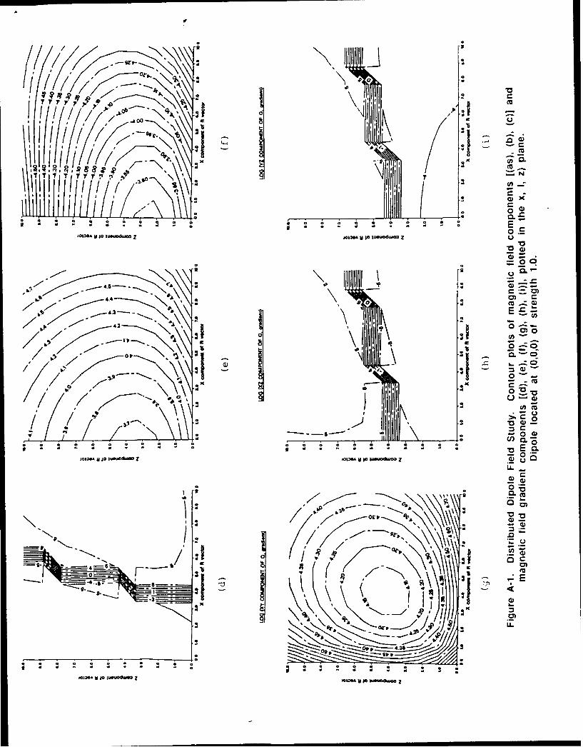
In preparation for the steering algorithm tests we made a study of the field B and

field gradient Q resulting from different magnetic dipole distributions as shown in Fig. 5.

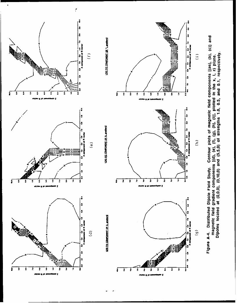
The following four figures (Figs. A-I through Fig. A-4) show some sample field and

gradient distributions. In these figures a grid of 10 x 10 x 10 points is used and the field

vector and gradient matrix were calculated at each point. In each case considered, a cut is

taken through the y-axis at y = I and the values of the fields at the 100 points in the (x, y =

1. z) plane are shown.

The basic format of the figures is as follows: the top three views in each figure (a,

b, c) show the equal magnetic field contour lines of the components Bx, BY. Bz.

respectively. The next six views (d, e, f, g, h, i) show the equal magnetic field gradient

contour line- Qxx, Qyy, Qzz, Qxy, Qxz, Qyz, respectively. The other components are

redundant because of symmetry. In each figure the logarithm of the value is actually

plotted.

20

z z.. ....z. .

(0,. 0,.0).=.. 1..0.0.).0 1, 0

.. ... =1.....0........................ ...

... (10,0,0)..... 2.. . 5 .. ...............

..-.- ..... ( d).. .. ..

Figure ..... Loaino.Df.etMantcDpoe.sUedi.h.agei iland.. Gradien Cotu.losi.ig.6Trog.6.... ... 21

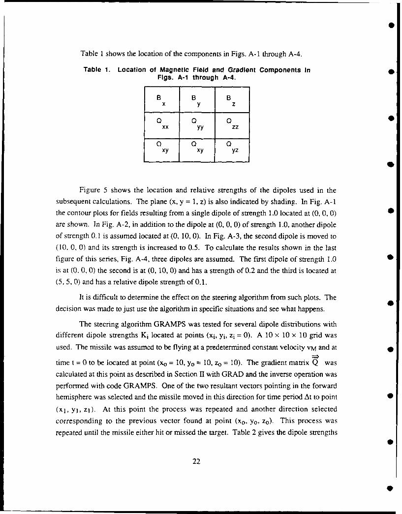
Table I shows the location of the components in Figs. A-I through A-4.

Table 1. Location of Magnetic Field and Gradient Components InFigs. A-1 through A-4.

B B Bx y z

xx yy zz

o Q axy xy yz

Figure 5 shows the location and relative strengths of the dipoles used in the

subsequent calculations. The plane (x, y = 1, z) is also indicated by shading. In Fig. A-i

the contour plots for fields resulting from a single dipole of strength 1.0 located at (0, 0, 0) 0are shown. In Fig. A-2, in addition to the dipole at (0, 0, 0) of strength 1.0, another dipole

of strength 0.1 is assumed located at (0, 10, 0). In Fig. A-3, the second dipole is moved to(10, 0, 0) and its strength is increased to 0.5. To calculate the results shown in the lastfigure of this series, Fig. A-4, three dipoles are assumed. The first dipole of strength 1.0is at (0, 0, 0) the second is at (0, 10, 0) and has a strength of 0.2 and the third is located at

(5, 5, 0) and has a relative dipole strength of 0.1.

It is difficult to determine the effect on the steering algorithm from such plots. The

decision was made to just use the algorithm in specific situations and see what happens.

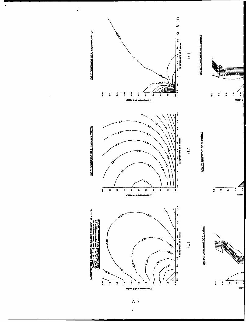
The steering algorithm GRAMPS was tested for several dipole distributions with

different dipole strengths Ki located at points (xi, yi, zi = 0). A 10 x 10 x 10 grid was

used. The missile was assumed to be flying at a predetermined constant velocity vM and at

time t = 0 to be located at point (xo = 10, Yo = 10, Z = 10). The gradient matrix Q was

calculated at this point as described in Section II with GRAD and the inverse operation was

performed with code GRAMPS. One of the two resultant vectors pointing in the forwardhemisphere was selected and the missile moved in this direction for time period At to point 0

(xl, yj, z1). At this point the process was repeated and another direction selected

corresponding to the previous vector found at point (xo, Yo, zo). This process was

repeated until the missile either hit or missed the target. Table 2 gives the dipole strengths2

22

I' 9

Table 2. Dipole Strength and Location Used for the Calculations ShownIn Figs. A-5 through A-13

Dipole Location Results ShownDipole Strengths (x, y, z) in Figure No.

1.0 (0,0,0) A-5

1.0 (0,0,0) A-60.1 (10,0,0)

1.0 (0,0,0) A-70.5 (10,0,0)

1.0 (0,0,0) A-80.1 (0, 10,0)

1.0 (0,0,0) A-90.2 (0,10,0)

1.0 (0,0,0) A-100.1 (0,10,0)0.1 (5,5,0)

1.0 (0,0,0) A-1I0.2 (0, 10, 0)0.1 (5,5,0)

1.0 (0,0,0) A-120.1 (0,10,0)0.2 (5,5,0)

1.0 (0,0,0) A-130.2 (0,10, 0)0.2 (5,5,0)

and locations used in a number of steering calculations and Figs. A-5 through A-15 show

the results of the calculations. In each figure, drawing (a) shows the initial vectors

indicated by a V, a', and b', and drawings (b) and (c) show paths taken as guided by the

algorithm GRAMPS. Note that although a symmetric situation was selected setting initial

conditions for the run shown in Fig. A-14, the algorithm still guides the missile to a target.

By symmetry consideration one might expect the missile to be guided between the targets.

It seems, however, that a slight numerical error breaks the symmetry and prevents this

23

I

from happening. In a real situation in the field we expect that this would also occur andthat slight perturbations in the fields would break the symmetry and force the missile to one

of the two targets.

Our limited sample shows that:

1. The steering algorithm works when the target is isolated from decoys. Whendecoys are present, the steering algorithm can be misled as shown in Fig. 10(c)and (d). In this case the decoy of strength K2 = 10 was 10 units away from

the starting point or ! times closer than the target. Since the dipole field goes

1like 3 this means that the interaction between target and sensor and

(distance)

decoy and sensor is in the ratio of ! 2 The decoy has a stronger attraction for

the target. 0

2. Either of the vectors a or b pointing in the forward hemisphere will direct orsteer the missile to the desired target.

3. It seems that the size of the angle between the vectors from the inverse solutionmay be a good indication of the steering effectiveness. If the two vectors thatpoint in the forward direction subtend on angle < 90 deg the steering will besuccessful. If this angle is > 90 deg a false target will be reached.

Clearly, further analysis is required. The present results only point the ways tomore simulations and analysis. These results, however, do indicate feasibility of steering

by using the gradiometer measurements.

24

• , m um m m m nmn m m n l~lanl~nnl ,, mnn l n

V. COUNTERMEASURES

The magnetic SQUID gradiometer tank seeker could be overcome by

1. Building tanks out of a nonmagnetic alloy,

2. Reducing the signature of magnetized tanks (deperming and degaussing) belowa measurable level,

3. Introducing false signatures,

4. Providing decoys to simulatc the tank's magnetic signature and divert theseeker.

As far as we know there are no tanks constructed solely from nonmagnetic material,

and it is not Lkely that this can be done in the foreseeable future. Ceramic armor is being

used, but other components of a tank are not built completely out of ceramic or non-

magnetic material.

Degaussing and deperming are well developed procedures used by the Navy to

protect surface ships and submarines from mines. Deperming removes some of the

permanent magnetization of the vessel produced during material processing andmanufacture. The effect lasts for about two years, at which point the process can be

repeated. Degaussing has to be performed continuously because it removes the induced

field due to the earth's field. This has to be done on demand and has to be customized to

the earth's field conditions.

Degaussing with coils en a surface vessel can be accomplished easily down to

0 20 percent of the induced magnetization (vertical component). With a lot more effort, a

reduction down to 5 percent is predicted. For submarines, degaussing is not practiced

because of the weight of coils and power requirements. Deperming is more practical and is

used for both surface vessels and submarines.

For tanks, no operational system for reducing the magnetic signature by degaussing

or deperming exists. This technology has been evaluated and a deperming cage constructed

for test purposes. Reduction down to 20 percent of original value has been obtained.

Clearly, this number could be improved, but the cost and operational utility has to beestablished. The Army seems to be more interested in signature modification designed to

25

trigger mines well ahead of tanks than in signature reduction. A lot of work has gone into

this effort. How well these signature modification techniques and signal reduction

techniques will actually work in the field to countermeasure the seeker has to be determined

through tests, evaluation, and further analysis.

Other possible countermeasures include the use of permanent or electromagnetsused as "flares" to distract the seeker. For the permanent magnet, it is simple to compute 0

the required size of the decoy.

Assume that the decoy is made from a magnetic material with a permanentmagnetization M (B = 47tM). The dipole moment of such a decoy is independent of the

details of the shape of the object and is given by the product of M and the volume. This 0can be seen by the following example. Consider a cylinder with cross-sectional area A,

and length L, with the magnetization M oriented along the cylinder axis. This is equivalent

for purposes of calculating the external field, to a surface current (in cgs units) K = cM.

The dipole moment is given by m = IA/c = KLA/c = MAL = M Volume. In general, the 0dipole moment of the material is given by m = J M dV = M Volume.

The dipole moment of the target was estimated (conservatively) as miarget =

BoR3 , with R taken as 1 m. For a permanent magnet decoy, mdecoy > mtargeO or MdecoyVdecoy > BoR 3 . For Swedish iron, an inexpensive magnetic material, M 103 0

corresponding to B - 12,000 gauss. Since BoR 3is approximately unity, Vdecoy 10- 3

m3 = 103 cm 3 (1 liter). Each of these decoys would therefore weigh about 8 kg.

These would have to be discharged at roughly 100-m intervals to be effective as decoys. In

10 kn, about a ton of decoys would be needed. More exotic material may raise M by an

order of magnitude (decreasing the volume by the same amount), but would increase the

cost.

This is close to the absolute limit to be expected if all the (relevant) spins in the

material were aligned. The magnetic moment per spin is eh/47tmc = 0.93 x 10- 20 gauss-

cm 3 . As an order of magnitude estimate, one may take two spins per atom and 1023

atoms/cm 3 , this yields Mlimit = 1.8 x 103. Therefore, no material is likely to extend this

limit significantly. The use of an electromagnet is unlikely to improve the values; an air

core magnet will have a lower field than one with a permeable core, and these will be

subject to the same limits as the permanent magnets.

26

VI. SUMMARY AND CONCLUSIONS

We have looked nt the feasibility of using a squid gradicm-eter as a sersor fcr an

antitank missile terminal guidance system. It is well known that inversion of the

gradiometer signal (from a collection of magnetic dipoles) gives an ambiguous result for the

direction of the target; four vectors in pairs pointing in opposite directions. For this reasonthe determination of the magnetic gradient in general would not be a very useful

measurement for a tank detection and guidance system, without additional information.

In our application, some additional information is available and two directions can

be selected from the four derived vectors. It turns out that both vectors lead to the target by

different routes when our algorithm is applied. We have performed simulations of missileguidance assuming various target and decoy magnetic strengths and spatial disnuibutions.

How well the algorithm works depends on the relative signal strengths and distances to

missile of the target and decoy. Several representative situations have been investigated.

We also estimated the range of application of the SQUID gradiometer system. For

an isolated tank with only an induced moment due to the earth's field, the approximate

distance from the target at which a SQUID gradiometer can begin to guide the missile is

150 m. Thus, for the guidance system to be effective, the missile nas to be shot into a

"bucket" 300 m i, diameter with the target in the center.

Our results show that the principle of inverting a gradiometer signal to obtain

guidance for a missile designed to attach a magnetic target is sound. Whether the system

can be made practical depends on the feasibility of building a SQUID from high

temperature superconductive material with low noise characteristics at temperatures high

enough so that lightweight refrigeration is possible. Since work on SQUIDS is going on

now, the answers to these questions are forthcoming.

P After questions regarding SQUID characteristics and refrigeration requirements are

resolved, questions regarding missile dynamics have to be addressed. Clearly, the missile

speed and maneuverability have to be designed around the sensor. We do not expect that

0

27

10

the sensor could be merely adapted to an existing missile. Finally, the question of

countermeasures has been addressed, but further in-depth work in this area has to be

initiated.

28

REFERENCES

1. W. Podney arid R. Sager, "Measurement of Fluctuating Magnetic GradientsOriginating From Oceanic Internal Waves," Science, Vol. 205, pp. 1381-1382,September 1979.

2. W. Podney and R. Sager, Measurement of Fluctuating Magnetic Gradients OverCoastal Waters, Physical Dynamics, Inc., La Jolla, California, March 1980.

3. T.G. Gamble, W.M. Goubau, and John Clarke, Magnetolellurics With a RemoteMagnetic Reference, Lawrence Berkeley Laboratory Report LBL-7032, January 1978.

4. J.E. Zimmerman and W.H. Campbell, "Tests of Cryogenic SQUID for GeomagneticField Measurements," Geophysics, Vol. 40, No. 2, pp. 269-284, April 1975.

5. M.B. Ketchen, W.M. Goubau, and J. Clarke, "Superconducting Thin-FilmGradiometer," J. Appl. Phys. 49(7), pp. 4111-4116, July 1978.

6. B. Balko, L. Cohen, R. Collins, J. Hove, J.F. Nicoll, "Central Research ProjectReport on Superconductivity (FY 1987)," IDA Memorandum Report M-468, May1988.

7. F.S. Grant and G.F. West, Interpretation Theory in Applied Geophysics, McGrawHill Book Co., 1965.

8. Mining Geophysics, Vol. 11, The SEG Mining Geophysics Volume EditorialCommittee, D.A. Houser, et al., Assoc. Eds., published by the Society of ExplorationGeophysicists, Tulsa, Oklahoma, 1966.

9. W.M. Wynn, C.P. Frahm, P.J. Carroll, R.H. Clark, J. Wellhoner, and W.J. Wynn,IEEE Trans. Magn., MAG-1 1 701, 1975.

10. T.D. Jackson, Classical Electrodynamics, John Wiley & Sons, Inc., New York,1962.

P

29

• i I

I

I

APPENDIX

I

S

S

S

S

S

S

S

A-i

S

P.B

I ,/~ a

P/

TF/ //V J 71

q 9 i! 9'

so,.

Owe-- -.--. '66 aw loj suawaflm

/ ~ A-3

Cv 0

*c 0

-00-c.

zc

ac

4.4 N4j 0

E\ S0 %

-42I v IPA c

10'' (D U

0 ~~~ 0 0 CC

CL

4; 46 1; o E 1

LLE

~ 05

%. bp

0) z

4 c - -S-;

MR'V£ U,080 ~~0

E E 00

0 0 0

(. 0-0

..............

xno@ W 0'woum M4

//

Wi,@A vF oo w wo o 7 r.

5A-5

4p 0

Il CL

-o E

Poo v o no.o*

0 Wc

a~~~~ a aL0

a~~~o c4 E. .4 - - 0

IC *A V OD iU UO&0 7R6 00e ow

"b z

Of -C \ I -1 1. , 1 0 ,//

M130A N 0 luoIJ0um0* Z t

A-7

al I

a a/ 4) Uii, '

VIL 4:,I

0~~ 0med Z MM M 00 0Modl 2

b cc -Z-

81 r-11

4, 0

/ 0o

lb~ CD

0 ~0G

mcCui

4t

x .xa-

10 no edP r .4 0 W *A %

Ore

\U

ILI

^:PDA ¥ jo "ueuO 00 0

7 A-

/ ,

/ -- -/.*

22///: :2--5 2 ;

"7 / C°.

i\ '

A-9

CL

0i

- -

C-

IIE S

& w v '~ so -M60ZvJommw

II CU.'U QW;

E EL

sew 0 rpto

Sa

0

.. 4

0b

4

t' % t.4

'o4' (a)

4.

Figure A-5. Simulation of steering by gradiometer Initial conditions with derived

vectors , b, a' and b' are shown In (a), and missile trajectories following vectors

a and b are shown In (b) and (c). A magnetic dipole of strength K =1.0

Is assumed to be located at (0,0,0) In this calculation.

SA-1 I

0.0

0

040

0


vectors a, b, a' and b' are shown In (a), and missile trajectories following vectors

a and b are shown In (b) and (c). Magnetic dipoles of strengths K1 = 1.0 andK2 = 0.1 are assumed to be located at point (0,0,0) and (10,0,0), respectively.

A-12

iI

(b)

,1 ,(.)

I

Figure A-7. Simulation of steering by gradlometer Initial conditions with derived

vectors a, b, a' and b' are shown in (a), and missile trajectories following vectors

aand b are shown In1 (b) and (c). Magnetic dipoles of strengths K, = 1.0 and

K2 = 0.5 are assumed to be located at point (0,0,0) and (10,0,0), respectively.

A-13

0"I*

0

- II

0

eui' (b)

a0

1.' (C)



a and b are shown in (b) and (c). Magnetic dipoles of strengths Kj = 1.0 andK2 = 0.1 are assumed to be located at point (0,0,0) and (0,10,0), respectively.

A-14

0

.14

1.

0

44

14

" ' (C)

Figure A-9. Simulation of steering by gradlometer Initial conditions with derived


0 a and b are shown In (b) and (c). Magnetic dipoles of strengths K1 = 1.0 and

K2 = -0.2 are assumed to be located at point (0,0,0) and (0,10,0), respectively.

A-15

0

a0

4..

'14'4 a

.. I

10.4 (a)

(b)

-0

Figure A-10. Simulation of steering by gradiometer Initial conditions with

derived vectors a, b, a' and b' are shown In (a), and missile trajectories

following vectors a and b are shown In (b) and (c). Magnetic dipoles ofstrengths K1 = 1.0, K2 = -0.1 and K3 = 0.1 are assumed to be located

at point (0,0,0), (0,10,0) and (5,5,0), respectively.

A- 160

0 3.4'4 '4

0.4 *, (a)

'4 (b)

0-3

14. (c)

Figure A-11. Simulation of steering by gradlometer Initial conditions with

derived vectors a, b, a' and b' are shown In (a), and missile trajectories

following vectors a and b are shown In (b) and (c). Magnetic dipoles ofstrengths K1 = 1.0, K2 = -0.2 and K3 = 0.1 are assumed to be located

at point (0,0,0), (0,10,0) and (5,5,0), respectively.

A-17

'*., (a)

aS -0

1.4

100

(C)


derived vectors a, b, a' and b' are shown In (a), and missile trajectories following

vectors a and b are shown In (b) and (c). Magnetic dipoles of strengthsK, = 1.0, K2 = 0.1 and K3 =0.2 are assumed to be located at point

(0,0,0), (0,10,0) and (5,5,0), respectively.

A-18 0

(a)

II

64 4 ~ (b)

qk

(C)


I derived vectors a, b, a anWb are shown In (a), and missile trajectories following

vectors a and b are shown In (b) and (c). Magnetic dipoles of strengthsKI = 1.0, K2 =0.2 and K3 = 0.2 are assumed to be located at point

(0,0,0), (0,10,0) and (5,5,0), respectively.

1A 149

.,f 'I- ,r

aQa Cb)

I Q4 4

(C)Figure A-14. Simulation of steering by gradometer Initial conditions with

derived vectors a, b, a' and b' are shown In (a), and missile trajectories following•

vectors a and b are shown In (b) and (c). Magnetic dipoles of strengthsK1 = 1.0 and K2 = 1.0 are assumed to be located at point

(0,-5,0) and (0,5,0), respectively.A-20

S (a)

~*% * ~ ~ - (b)

Figure A-15. Simulation of steerIng by gradiometer Initial conditiors with

* derived vectors a, b, an b' are shown in (a), and missile trajectories following

vectors a and b are shown In (b) and (c). Magnetic dipoles of strengthsK1 = 1.0 and K2 =0.2 are assumed to be located at point

(0,-7,0) and (0,3,0), respectively.

* A-21