i. introduction - columbia universityxg2285/proximity.pdf · thank my advisor, holger mueller; ......

PROXIMITY AND INVESTMENT: EVIDENCE FROMPLANT-LEVEL DATA*

Xavier Giroud

Proximity to plants makes it easier for headquarters to monitor and ac-quire information about plants. In this article, I estimate the effects of head-quarters’ proximity to plants on plant-level investment and productivity. Usingthe introduction of new airline routes as a source of exogenous variation inproximity, I find that new airline routes that reduce the travel time betweenheadquarters and plants lead to an increase in plant-level investment of 8% to9% and an increase in plants’ total factor productivity of 1.3% to 1.4%. Theresults are robust when I control for local and firm-level shocks that couldpotentially drive the introduction of new airline routes, when I consider onlynew airline routes that are the outcome of a merger between two airlines or theopening of a new hub, and when I consider only indirect flights where eitherthe last leg of the flight (involving the plant’s home airport) or the first leg ofthe flight (involving headquarters’ home airport) remains unchanged. Moreover,the results are stronger in the earlier years of the sample period and for firmswhose headquarters is more time-constrained. In addition, they also hold at theextensive margin, that is, when I consider plant openings and closures.JEL Codes: D24, G31.

I. Introduction

Proximity facilitates monitoring and access to information.For instance, venture capitalists are more likely to serve onthe boards of local firms, where monitoring is easier (Lerner1995). Likewise, mutual fund managers are more likely to holdshares of local firms—and they earn significant abnormal returnsfrom these investments—suggesting ‘‘improved monitoring

*This article is based on my dissertation submitted to New York University. Ithank my advisor, Holger Mueller; the editors, Jeremy Stein, Andrei Shleifer, andLarry Katz; three anonymous referees; as well as Viral Acharya, AshwiniAgrawal, Allan Collard-Wexler, Carola Frydman, Xavier Gabaix, Kose John,Marcin Kacperczyk, Andrew Karolyi, Leonid Kogan, Anthony Lynch, JavierMiranda, Adair Morse, Dimitris Papanikolaou, Adriano Rampini, MichaelRoberts, Alexi Savov, Philipp Schnabl, Antoinette Schoar, Amit Seru, DanielWolfenzon; and seminar participants at MIT, Chicago, Stanford, NYU,Wharton, Kellogg, UCLA, Yale, Duke, Ohio State, Cornell, and USC for valuablecomments and suggestions. The research in this article was conducted while theauthor was a Special Sworn Status researcher of the U.S. Census Bureau at theNew York and Boston Census Research Data Centers. Any opinions and conclu-sions expressed herein are those of the author and do not necessarily representthe views of the U.S. Census Bureau. All results have been reviewed to ensurethat no confidential information is disclosed.

! The Author(s) 2012. Published by Oxford University Press, on behalf of Presidentand Fellows of Harvard College. All rights reserved. For Permissions, please email:[email protected] Quarterly Journal of Economics (2013), 861–915. doi:10.1093/qje/qjs073.Advance Access publication on December 19, 2012.

861

at MIT

Libraries on A

pril 28, 2013http://qje.oxfordjournals.org/

Dow

nloaded from

http://qje.oxfordjournals.org/

capabilities or access to private information of geographicallyproximate firms’’ (Coval and Moskowitz 1999, 2001, 812).Finally, banks located closer to their borrowers are more likelyto lend to informationally difficult borrowers, for example, bor-rowers without any financial records (Petersen and Rajan 2002;Mian 2006; Sufi 2007).

All of these examples come from arm’s-length transactions.Much less, if anything, is known about the role of proximitywithin firms. For instance, is it true that—in analogy to the find-ings in the mutual funds and banking literatures—headquartersis more likely to invest in plants that are located closer to head-quarters? Does proximity to headquarters improve plant-levelproductivity? Understanding plant-level investment and prod-uctivity is important, not least because they affect economicgrowth.1 One difficulty in answering these questions is thatthey require data on the locations of plants and headquarters.Another, more serious issue is that the locations of plants andheadquarters are choice variables. Accordingly, commonly usedproxies for proximity—such as the physical distance betweenplants and headquarters—are likely to be endogenous, makingit difficult to establish causality.

I attempt to address both of these issues. For the first issue, Iuse plant-level data provided by the U.S. Census Bureau for themanufacturing sector for the period 1977 to 2005, which includethe locations of plants and headquarters. For the second issue, Inotice that the main reason empirical studies are interested in(geographical) proximity is because it proxies for the ease of moni-toring and acquiring information. I argue that a more directproxy is travel time. For instance, a plant may be located faraway from headquarters, yet monitoring may be easy, becausethere exists a short, direct flight. Conversely, a plant may be

1. Anecdotal evidence suggests that proximity to headquarters is a potentiallyimportant determinant of plant-level investment. For instance, when Tesla Motorsdecided on the location of a manufacturing plant to produce its electric Tesla road-ster, it announced that the plant would be located ‘‘as close to our headquarters aspossible,’’ citing as a reason ‘‘to keep better control over production’’ (Silicon Valley/San Jose Business Journal, June 30, 2008). As for the effects of proximity on prod-uctivity, Ray Kroc, the founder of McDonald’s, writes in his autobiography: ‘‘Onething I liked about that house was that it was perched on a hill looking down on aMcDonald’s store on the main thoroughfare. I could pick up a pair of binoculars andwatch business in that store from my living room window. It drove the managercrazy when I told him about it. But he sure had one hell of a hard-working crew!’’(Kroc 1992, 141).

QUARTERLY JOURNAL OF ECONOMICS862

at MIT

Libraries on A


Dow

nloaded from


located in the same state as headquarters, yet monitoring may becostly, because it involves a long and tedious road trip. Of course,in the cross-section, geographical proximity and travel time arehighly correlated. However, the advantage of using travel time isthat it entails plausibly exogenous variation, allowing me to ad-dress the endogeneity issue.

Precisely, I combine the census plant-level data with airlinedata from the U.S. Department of Transportation, which containinformation about all flights that have taken place between anytwo airports in the United States. The specific source of exogen-ous variation that I exploit is the introduction of new airlineroutes that reduce the travel time between headquarters andplants. Using a difference-in-differences approach, I find thatthe introduction of new airline routes leads to an increase inplant-level investment of 8% to 9%, corresponding to an increasein capital expenditures of $158,000 to $177,000 (in 1997 dollars).Moreover, I find that plants’ total factor productivity increases by1.3% to 1.4%, corresponding to an increase in plant-level profits of$275,000 to $296,000 (in 1997 dollars).

My identification strategy can be illustrated with a simpleexample. Consider a company headquartered in Boston with aplant in Memphis. In 1985, the fastest way to travel fromBoston to Memphis was an indirect flight with one stopover inAtlanta. In 1986, Northwest Airlines opened a new hub inMemphis and started operating direct flights between Bostonand Memphis. The introduction of this new airline route substan-tially reduced the travel time between the Boston headquartersand the Memphis plant and is therefore coded as a ‘‘treatment’’ ofthe Memphis plant.2

An important concern is that local shocks in the plant’s vicin-ity could be driving both the introduction of new airline routesand plant-level investment. For instance, suppose the local econ-omy in Memphis is booming. As a result, the company headquar-tered in Boston may find it more attractive to increase investmentat its Memphis plant. At the same time, airlines may find it moreattractive to introduce new flights to Memphis (e.g., because oflobbying by local plants). In this case, finding a positive treatmenteffect would be a spurious outcome of an omitted shock in the

2. Overall, there are 10,533 plants in my sample that experience a reduction inthe travel time to headquarters due to the introduction of new airline routes.

PROXIMITY AND INVESTMENT 863

at MIT

Libraries on A


Dow

nloaded from


Memphis area. Fortunately, because a treatment is uniquelydefined by two (airport) locations—the plant’s and headquarters’home airports—I can control for such local shocks, making theidentification even tighter. Specifically, I include metropolitanstatistical area (MSA)–year controls in all my regressions.Similarly, to account for omitted shocks at the firm level, I includefirm-year controls in all my regressions. Both types of controls areidentified here, because not all local plants have their headquar-ters in the same city or region and not all plants of a given firmare affected by the introduction of a new airline route,respectively.

Although the inclusion of MSA- and firm-year controlsaccounts for omitted local and firm-level shocks, it remains thepossibility of an omitted shock that is specific to a single plant—that is, the shock does not affect other plants within the sameregion or firm. I address this issue in three ways. First, I considerthe dynamic effects of the introduction of new airline routes. If anew airline route is the (endogenous) outcome of a preexistingplant-specific shock, then I should find an ‘‘effect’’ of the treat-ment already before the new airline route is introduced. However,I find no such effect. Second, I show that my results are robustwhen I consider only new airline routes that are the outcome of amerger between two airlines or the opening of a new hub.Arguably, it is less likely that a shock to a single plant wouldtrigger an airline merger or a hub opening. Third, I show thatmy results are robust when I consider only indirect flights whereeither the last leg of the flight (involving the plant’s home airport)or the first leg of the flight (involving headquarters’ home airport)remains unchanged. Arguably, it is less likely that a single plantor headquarters can successfully lobby for the introduction of anew flight elsewhere, that is, a flight that does not involve itsrespective home airport.

A limitation of my study is that by design, it relies onexogenous variation in travel time, not variation in monitoringor access to information. With this caveat in mind, I think it isplausible that a travel time reduction leads to an improvement inmonitoring and information acquisition and, as a result, to anincrease in plant-level investment and productivity. For instance,monitoring by headquarters may induce higher effort by plantmanagers and workers (see the McDonald’s example in note 1),thus improving the plant’s productivity and, along with it, theplant’s marginal return on investment. Moreover, just like


at MIT

Libraries on A


Dow

nloaded from


mutual fund managers may face less uncertainty with respect tolocal stocks, headquarters may face less uncertainty with respectto local projects. Consequently, headquarters may be in a betterposition to evaluate local projects and, as a result, assign a largerinvestment budget to them.

That being said, there are alternative stories that I cannotrule out. For instance, visiting the plant more often may allow theCEO to give better advice, thereby improving the plant’s product-ivity and, by implication, its marginal return on investment. Orthe plant managers may simply get a better sense of the com-pany’s needs. Or it may improve the plant managers’ morale,who may think they have a better chance of getting promoted iftheir actions become more visible to headquarters. Or headquar-ters may devote more of its ‘‘limited attention,’’ for example, in thebudget allocation process, to plants that have become more sali-ent to it.3 Although all of these alternative stories can be broadlycategorized under the notion of ‘‘information transmission,’’ theyarguably have a different flavor. Importantly, however, all ofthem have to do with proximity, which is the main hypothesisexplored in this article. Moreover, as the new airline routes arecommercial (not cargo), they also all have to do with personaltravel. Thus, the reason for plant-level investment increases isnot, for example, that it becomes cheaper to ship equipment to theplant.

In the final part of this article, I provide auxiliary evidencethat a reduction in travel time facilitates monitoring and infor-mation acquisition. For instance, I show that my results arestronger for plants whose headquarters is more ‘‘time-constrained,’’ based on the notion that time constraints limitthe ability to monitor and gather information about plants.Likewise, I show that my results are stronger in the earlieryears of the sample period, where other, nonpersonal means ofinformation transmission (e.g., Internet, corporate intranet,video conferencing) were either unavailable or less developed. Ialso examine what happens at the ‘‘extensive margin,’’ that is,with respect to plant openings and closures. Specifically, I showthat companies whose headquarters is more time-constrained aremore likely to open new plants—and are less likely to close

3. For models of limited attention, see Gabaix et al. (2006), Gennaioli andShleifer (2010), and Bordalo, Gennaioli, and Shleifer (2012). See also DellaVigna(2009, Section 4.2) for a survey of the literature.


at MIT

Libraries on A


Dow

nloaded from


existing plants—in close proximity to headquarters. Likewise, Ishow that over time—as innovations in information technologyhave reduced the need to personally travel to plants—firms havebecome more likely to open new plants at remote locations andclose existing plants at proximate locations. The latter result isconsistent with Petersen and Rajan’s (2002) finding that, owing toinnovations in information technology, the distance betweensmall business borrowers and their lenders has increased overtime.

The results in this article have important policy and welfareimplications. From a policy perspective, they point to an import-ant externality of transportation infrastructure: the facilitationof monitoring and information flows within firms. That beingsaid, this externality seems to have become less important inthe later years of the sample period, where innovations in infor-mation technology have facilitated information flows both withinand across company units. Likewise, the results suggest thatstate or regional competition for firms to set up new plants maynot be a zero-sum game. Specifically, if distant states or regionsprevail in the competition—for example, because they can offerbetter tax breaks or other incentives—plant-level investment andproductivity may be lower than if relatively proximate states orregions had won. Finally, a possible welfare implication of myresults is that firms may be induced to locate plants subopti-mally—that is, closer to headquarters than would be optimal ina frictionless world with perfect and symmetric information—forthe sole purpose of facilitating monitoring and informationtransmission.

The rest of this article is organized as follows. Section II de-scribes the data and empirical methodology. Section III presentsthe main results. Section IV contains robustness checks. SectionV considers heterogeneity in the treatment effect. Section VI con-siders plant openings and closures. Section VII concludes.Appendix A and Appendix B provide information regarding theconstruction and measurement of variables.

II. Data

II.A. Data Sources and Sample Selection

Plant-Level Data. The data on manufacturing plants are ob-tained from three different data sets provided by the U.S. Census


at MIT

Libraries on A


Dow

nloaded from


Bureau. The first data set is the Census of Manufactures (CMF).The CMF covers all U.S. manufacturing plants with at least onepaid employee. The CMF is conducted every five years in yearsending with 2 and 7 (‘‘Census years’’). The second data set is theAnnual Survey of Manufactures (ASM). The ASM is conducted inall non-Census years and covers a subset of the plants covered bythe CMF: plants with more than 250 employees are included inevery ASM year, whereas plants with fewer employees are ran-domly selected every five years, where the probability of being se-lected is higher for larger plants. Although the ASM is referred toas a ‘‘survey,’’ reporting is mandatory, and fines are levied for mis-reporting. The CMF and ASM cover approximately 350,000 and50,000 plants per year, respectively, and contain informationabout key plant variables, such as capital expenditures, totalassets, value of shipments, material inputs, employment, industrysector, and location. The third data set is the LongitudinalBusiness Database (LBD), which is compiled from the BusinessRegister. The LBD is available annually and covers all U.S. busi-ness establishments with at least one paid employee.4 The LBDcontains longitudinal establishment identifiers along with data onemployment, payroll, industry sector, location, and corporate af-filiation. I use the longitudinal establishment identifiers to con-struct longitudinal linkages between the CMF and ASM.

Given that the LBD covers the entire U.S. economy, it alsocontains information about non-manufacturing establishments ofcompanies that have plants in either the CMF or the ASM. I usethis information to construct firm-level variables, such as thetotal number of employees and the number of establishmentsper firm. For my analysis, the most important firm-level variableis the ZIP code of the company’s headquarters. At the firm level,the Census Bureau distinguishes between single- and multi-unitfirms. Single-unit firms consist of a single establishment, whichmeans headquarters and the plant are located in the same unit.Multi-unit firms consist of two or more LBD establishments, withone establishment being the company’s headquarters.

To determine the location of headquarters, I supplement theLBD with data from two other data sets provided by the CensusBureau: the Auxiliary Establishment Survey (AES) and the

4. An establishment is a ‘‘single physical location where business is conducted’’(Jarmin and Miranda 2003, 15). Establishments are the economic units used in theCensus data sets.


at MIT

Libraries on A


Dow

nloaded from


Standard Statistical Establishment List (SSEL). The AES con-tains information on non-production (‘‘auxiliary’’) establish-ments, including information on headquarters. The SSELcontains the names and addresses of all U.S. business establish-ments. Appendix A outlines the procedure used to obtain the lo-cation of headquarters from these data sets. The main source ofinformation about headquarters, the AES, is available every fiveyears between 1977 and 2002. To fill in the missing years, I usethe information from the latest available AES. Given that theCensus years are deterministic, this measurement error isunlikely to introduce any bias. It merely introduces noise intothe regression, which makes it harder for me to find any signifi-cant results.

My sample covers the period from 1977 to 2005. (The firstavailable AES year is 1977; 2005 is the last available ASM year.)To be included in my sample, I require that a plant have a min-imum of two consecutive years of data. Following common prac-tice in the literature (e.g., Foster, Haltiwanger, and Syverson2008), I exclude plants whose information is imputed from admin-istrative records rather than directly collected. I also excludeplant-year observations for which employment is either zero ormissing. Finally, to ensure that the physical distance betweenplants and headquarters is comparable across years, I excludefirms that change the location of their headquarters during thesample period. The results are virtually identical if these firmsare included.

The foregoing selection criteria leave me with 1,332,824plant-year observations. In my regressions, I use a 10-yearwindow around the treatment date, meaning treated plants areincluded from 5 years before the treatment to 5 years after thetreatment. Using a 10-year treatment window reduces my sampleonly slightly, leaving me with a final sample of 1,291,280plant-year observations. That being said, the length of the treat-ment window is immaterial for my results. All results are similarif I use a different treatment window or no treatment window atall, meaning all plant-year observations of treated plants areincluded either before or after the treatment.

Airline Data. The data on airline routes are obtained from theT-100 Domestic Segment Database (for the period 1990 to 2005)and ER-586 Service Segment Data (for the period 1977 to 1989),


at MIT

Libraries on A


Dow

nloaded from


which are compiled from Form 41 of the U.S. Department ofTransportation (DOT).5 All airlines operating flights in theUnited States are required by law to file Form 41 with the DOTand are subject to fines for misreporting. Strictly speaking, theT-100 and ER-586 are not samples: They include all flights thathave taken place between any two airports in the United States.

The T-100 and ER-586 contain monthly data for each airlineand route (segment). The data include, for example, the originand destination airports, flight duration (ramp-to-ramp time),scheduled departures, performed departures, enplaned passen-gers, and aircraft type.

II.B. Empirical Methodology

The introduction of new airline routes that reduce the traveltime between headquarters and plants makes it easier for head-quarters to monitor and acquire information about plants. Toexamine the effects on plant-level investment and productivity,I use a difference-in-differences approach. I estimate:

yijlt ¼ �i þ �t þ �� treatmentit þ �0 Xijlt þ "ijlt,ð1Þ

where i indexes plants, j indexes firms, l indexes plant location, tindexes years, yijlt is the dependent variable of interest (plantinvestment or productivity), ai and at are plant and year fixedeffects, treatment is a dummy variable that equals 1 if a newairline route that reduces the travel time between plant i andits headquarters has been introduced by time t, X is a vector ofcontrol variables, and e is the error term. Location is defined atthe MSA level.6 The main coefficient of interest is b, which meas-ures the effect of the introduction of new airline routes.

5. The T-100 Domestic Segment Database is provided by the Bureau ofTransportation Statistics. The annual files of the ER-586 Service Segment Dataare maintained in the form of magnetic tapes at the U.S. National Archives andRecords Administration (NARA). I obtained a copy of these tapes from NARA.

6. As defined by the Office of Management and Budget, an MSA consists of acore area that contains a substantial population nucleus together with adjacentcommunities that have a high degree of social and economic integration with thatcore. MSAs include one or more counties, and some MSAs contain counties fromseveral states. For instance, the New York MSA includes counties from four states:New York, New Jersey, Connecticut, and Pennsylvania. Because MSAs representeconomically integrated areas, they are likely to be affected by the same localshocks. By definition, the MSA classification is only available for urban areas.For rural areas, I consider the rural part of each state as a separate region. Thereare 366 MSAs in the United States and 50 rural areas based on state boundaries.


at MIT

Libraries on A


Dow

nloaded from


If the relationship between plants and headquarters is gov-erned by symmetric information and no agency problems, thenthe introduction of new airline routes might not matter. In allother cases, it might matter. For instance, headquarters mayinvest more in plants that are easier to monitor and are lesslikely to have private information.7 Likewise, better monitoringmay improve plant managers’ incentives, and learning about aplant may allow headquarters to improve the plant’s productiv-ity. On the other hand, if headquarters becomes ‘‘too well in-formed’’ or ‘‘monitors too much,’’ this may impair plantmanagers’ incentives to create new investment opportunities(Aghion and Tirole 1997) or work hard (Cremer 1995).

My identification strategy can be illustrated with a simpleexample. Suppose a company headquartered in Boston has aplant located in Memphis. In 1985, no direct flight was offeredbetween Boston Logan International Airport (BOS) and MemphisInternational Airport (MEM). The fastest way to connect bothairports was an indirect flight operated by Delta Airlines with astopover in Atlanta. In 1986, Northwest Airlines opened a newhub in MEM. As part of this expansion, Northwest started oper-ating direct flights between BOS and MEM as of October 1986.The introduction of this new airline route reduced the travel timebetween BOS and MEM and is consequently coded as a ‘‘treat-ment’’ of the Memphis plant in 1986.

To measure the effect of this treatment on, for example,plant-level investment, one could simply compare investment atthe Memphis plant before and after 1986. However, other eventsin 1986 might have also affected investment at the Memphisplant. For instance, there might have been a nationwide surgein investment due to favorable economic conditions or low inter-est rates. To account for this possibility, I include a control groupthat consists of all plants that have not (yet) been treated. Due tothe staggered nature of the introduction of new airline routes,

(The District of Columbia has no rural area.) For expositional simplicity, I refer tothese 416 geographical units as MSAs.

7. A standard result in the capital budgeting literature with asymmetric in-formation is that there is likely to be underinvestment under the optimal mechan-ism (e.g., Harris and Raviv 1996; Malenko 2011). See also Seru (forthcoming), whoprovides empirical evidence consistent with the idea that headquarters is less likelyto invest in projects that rely on division managers’ private information. Likewise,moral hazard, which can be alleviated through monitoring, typically leads to under-investment in equilibrium (e.g., Tirole 2006, chapters 3 and 4).


at MIT

Libraries on A


Dow

nloaded from


this implies a plant remains in the control group until it is treated(which, for some plants, may be never). I then compare the dif-ference in investment at the Memphis plant before and after 1986with the difference in investment at the control plants before andafter 1986. The difference between the two differences is the esti-mated effect of the introduction of the new airline route betweenBOS and MEM on investment at the Memphis plant.

Airlines’ decisions to introduce new routes depend on severalfactors, including economic and strategic considerations as wellas lobbying. As long as these factors are unrelated to plant-levelinvestment or productivity, this is not a concern. However, ifthere are (omitted) factors that are driving both the introductionof new airline routes and plant-level investment or productivity,then any relationship between the two could be spurious. I nowdiscuss how my identification strategy can account for suchomitted factors at the local, firm, and plant level.

Local Shocks. To continue with the example, suppose theMemphis area is booming. As a consequence, the company head-quartered in Boston may find it more attractive to increase in-vestment at the Memphis plant. At the same time, airlines mayfind it more attractive to introduce new flights to Memphis (e.g.,due to lobbying by local plants). Fortunately, because a treatmentis uniquely defined by two (airport) locations—the plant’s andheadquarters’ home airports—I can control for such localshocks, thus separating out the effects of the new airline routesfrom the effects of contemporaneous local shocks.

Suppose, for instance, that another plant, also located inMemphis, has its headquarters in Chicago. (The travel time be-tween Chicago and Memphis was not affected by the introductionof new airline routes during 1985 and 1986.) If investment at thisother Memphis plant also increases in 1986, then an increase ininvestment at the first Memphis plant (with headquarters inBoston) might not be due to the newly introduced airline routebetween MEM and BOS but due to a contemporaneous localshock in the Memphis area. In principle, I could control forsuch local shocks by including a full set of MSA fixed effects inter-acted with year fixed effects. However, doing so would require theinclusion of 416 MSAs�29 years = 12,064 additional fixed effects.Unfortunately, the computing resources at the Census ResearchData Center were insufficient to handle this task. I therefore


at MIT

Libraries on A


Dow

nloaded from


adopt the methodology used in Bertrand and Mullainathan(2003) and account for local shocks by including MSA-yearcontrols, which are computed as the mean of the dependent vari-able (e.g., plant-level investment) in the plant’s MSA in a givenyear, excluding the plant itself.8

An alternative way to account for local shocks is to focus onlyon new airline routes whose introduction is unlikely to be drivenby such shocks. Specifically, in a subset of cases, a new indirectflight replaces a previously optimal indirect flight, but the last legof the flight—that is, the leg involving the plant’s home airport—remains unchanged. For instance, suppose a (different) companyheadquartered in Boston has a plant in Little Rock. In 1985, thefastest way to connect BOS and Little Rock National Airport(LIT) was an indirect flight with stopovers in Atlanta (ATL) andMEM. In 1986, Northwest Airlines started operating directflights between BOS and MEM, with the effect that the previ-ously optimal indirect flight BOS-ATL-MEM-LIT is replacedwith a new, faster indirect flight BOS-MEM-LIT. Importantly,the last leg of the flight—that between MEM and LIT—remainsunchanged. Arguably, it is unlikely that a local shock in the LittleRock area would be responsible for the introduction of a new air-line route between BOS and MEM. As I show in robustnesschecks, I obtain similar results when I consider only new airlineroutes where the last leg of the flight remains unchanged.

Firm-Level Shocks. I am also able to control for firm-levelshocks. For instance, suppose the company headquartered inBoston has another plant in Queens in New York City. (Thetravel time between Queens and Memphis was not affected bythe introduction of new airline routes during 1985 and 1986.) Ifinvestment at the Queens plant also increases in 1986, then anincrease in investment at the Memphis plant might not be dueto the newly introduced airline route between MEM and BOSbut to a contemporaneous shock at the firm level. Analogousto the construction of the MSA-year controls, I can accountfor firm-level shocks by including firm-year controls, which are

8. Analternative approach would be touse a coarser definition of location, suchas the nine census regions. This would only require the inclusion of 9 regions� 29years = 261 additional fixed effects. I have done this, and all my results remainsimilar.


at MIT

Libraries on A


Dow

nloaded from


computed as the mean of the dependent variable across all of thefirm’s plants in a given year, excluding the plant itself.

Similar to the case of local shocks, an alternative way to ac-count for firm-level shocks is to focus only on new airline routeswhose introduction is unlikely to be driven by such shocks.Specifically, in a subset of cases, a new indirect flight replaces apreviously optimal indirect flight, but the first leg of the flight—that is, the leg involving headquarters’ home airport—remainsunchanged. As I show in robustness checks, I obtain similar re-sults when I focus only on this subset of new airline routes.

Plant-Specific Shocks. There is one remaining possibility:shocks that are specific to a single plant.9 Because such shocksdo not affect other plants in the same region, they cannot be ac-counted for by the inclusion of MSA-year controls. Likewise, asthe shocks do not affect other plants of the same company, theycannot be accounted for by the inclusion of firm-year controls. Iaddress this possibility in three different ways.

First, I consider the dynamic effects of the introduction ofnew airline routes. If a new airline route is the (endogenous) out-come of a preexisting plant-specific shock, then I should find an‘‘effect’’ of the treatment already before the new airline route isintroduced. However, I find no such effect. On the contrary, I findthat plant-level investment (productivity) increases only with alag of 6–12 (12–18) months after the introduction of the new air-line route, implying there is no effect either before or immediatelyafter.

Second, it could be that a new airline route is introduced inanticipation of a future plant-specific shock. Or it could be thatthe shock leads first to the introduction of a new airline route andonly later to an increase in plant-level investment (productivity).Both interpretations are consistent with the absence of preexist-ing trends. To address this issue, I show that my results are

9. For expositional simplicity, I refer to such shocks as ‘‘plant-specific shocks.’’Strictly speaking, this category encompasses any shock whose dimension is at theplant-headquarters level, that is, any shock that is collinear with the treatment.This includes, for example, ‘‘pair-specific’’ shocks to trade between the plant’s andheadquarters’ locations, in the sense that only plants in location A with headquar-ters in location B—but not plants in location A in general—are affected by theshock. Naturally, a shock that is specific to a single plant is also a pair-specificshock, given that each plant is associated with a unique headquarters’ location.


at MIT

Libraries on A


Dow

nloaded from


robust when I consider only new airline routes that are the out-come of a merger between two airlines or the opening of a newhub. Arguably, it is less likely that a shock to a single plant wouldbe responsible for an airline merger or a hub opening.

Third, I show that my results are robust when I consider onlyindirect flights where either the last or first leg of the flight re-mains unchanged. This addresses not only the possibility of localand firm-level shocks but also the possibility of shocks that arespecific to a single plant.

Finally, I should mention that I obtain similar results when Iconsider only small plants or plants of small firms. Arguably, it isless likely that small plants or firms can successfully lobby for theintroduction of a new airline route. By the same token, airlinesare less likely to respond to shocks affecting small plants or plantsof small firms. I should also point out that there are 10,533 plantsoverall in my sample that experience a reduction in travel timedue to the introduction of new airline routes. Even if it were truethat, in some cases, the new airline route was the outcome oflobbying by individual plants (or firms), this would still implythat the treatment is exogenous for the remaining 10,000+plants.

Miscellaneous Methodological Issues. In addition to account-ing for the possibility of local shocks, firm-level shocks, andplant-specific shocks, my empirical design can address severalother concerns.

(1) The time variation in travel time used to construct thetreatment dummy comes entirely from the introductionof new airline routes. In reality, travel time can alsovary for other reasons, such as the introduction of newroads, changes in speed limits, and the expansion ofrailroad networks. Unfortunately, lack of comprehen-sive data makes it difficult to account for these sourcesof travel time variation. Nevertheless, their omission isunlikely to affect my results. First, I show in robust-ness checks that my results are only significant forlarge reductions in travel time (at least two hoursround-trip), which almost always come fromlong-distance trips where air travel is the optimalmeans of transportation. Second, plants whose travel


at MIT

Libraries on A


Dow

nloaded from


time to headquarters is reduced through the expansionof roads and railroad networks are part of the controlgroup. Thus, to the extent that these sources of traveltime reduction lead to an increase in plant-level invest-ment (productivity), their omission would imply thatmy results understate the true effects of travel timereductions.10

(2) I do not consider the termination of existing airlineroutes, only the introduction of new airline routes.Terminations are much less frequent than introduc-tions. Moreover, as routes that are discontinued aremostly minor regional routes, the resulting increasein travel time is generally modest. That being said, Ishow in robustness checks that my results are un-changed if I account for the termination of existing air-line routes. Precisely, I augment the specification inequation (1) by adding a second treatment dummythat equals 1 whenever the termination of an existingairline route leads to an increase in travel time be-tween a plant and its headquarters. Including thissecond treatment dummy has no effect on the maintreatment dummy (see Table VII later).

(3) Some companies may own private jets. However, ifcompanies use private jets to fly to plants, then theintroduction of new airline routes should not matter.Although this is unlikely to introduce any systematicbias, it introduces noise into the regressions, making itonly harder for me to find any significant results.

(4) My sample spans 29 years of data (from 1977 to 2005).In my regressions, I use a 10-year treatment windowthat begins 5 years before the treatment and ends 5

10. I should note that large reductions in travel time through the expansion ofroads and railroad networks are less likely during my sample period, given thatmost of today’s road and railroad infrastructure was already in place before thebeginning of my sample in 1977. Most of the railroad network was built prior toWorld War I. The latest major extension of the road network was the completion ofthe Interstate Highway System. Construction began in 1956 after the enactment ofthe National Interstate and Defense Highways Act. By 1975, the system was mostlycomplete (Michaels 2008). In contrast, the airline industry was deregulated earlyduring my sample period (Airline Deregulation Act of 1978), which triggered anexpansion of airline routes in the following decades. Hence, most of the time seriesvariation in travel time during my sample period is due to changes in airline routes,not due to the expansion of roads and railroad networks.


at MIT

Libraries on A


Dow

nloaded from


years after the treatment. However, my results aresimilar if I use different treatment windows (6, 8, 12,14 years) or no treatment window at all, meaning allplant-year observations of treated plants are includedeither before or after the treatment.

(5) An important concern—especially with regard todifference-in-differences estimations—is that serial cor-relation of the error term can lead to understatedstandard errors. In my regressions, I cluster standarderrors at the MSA level. This clustering not only ac-counts for the presence of serial correlation within thesame plant, it also accounts for any arbitrary correl-ation of the error terms across plants in the sameMSA in any given year as well as over time. My resultsare similar if I cluster standard errors at the firm levelor at both the MSA and firm level. I also obtain similarresults if I collapse the data into two periods, beforeand after the introduction of a new airline route,using the residual aggregation method described inBertrand, Duflo, and Mullainathan (2004).

II.C. Definition of Variables

Measuring Investment. Investment is total capitalexpenditures divided by capital stock. Both the numerator anddenominator are expressed in 1997 dollars.11 Investment isindustry-adjusted by subtracting the industry median in agiven three-digit SIC industry and year.12 To mitigate the effectof outliers, I winsorize investment at the 2.5th and 97.5thpercentiles of its empirical distribution.

Measuring Productivity. My main measure of plant product-ivity is total factor productivity (TFP). TFP is the difference be-tween actual and predicted output. Predicted output is the

11. Capital expenditures are deflated by the four-digit SIC investment deflatorfrom the NBER-CES Manufacturing Industry Database. Appendix B describes howreal capital stock is constructed.

12. Instead of industry-adjusting investment, I could alternatively includeindustry-year controls, which are computed analogously to the MSA- and firm-yearcontrols. My results would be unchanged.


at MIT

Libraries on A


Dow

nloaded from


amount of output a plant is expected to produce for given levels ofinputs. To compute predicted output, I use a log-linear Cobb-Douglas production function (e.g., Lichtenberg 1992; Schoar2002; Bertrand and Mullainathan 2003; Syverson 2004; Foster,Haltiwanger, and Syverson 2008). Specifically, TFP of plant i inyear t is the estimated residual from the regression

yit ¼ �0 þ �kkit þ �llit þ �mmit þ "it,ð2Þ

where y is the logarithm of output and k, l, and m are the loga-rithms of capital, labor, and material inputs, respectively. Toallow for different factor intensities across industries and overtime, I estimate equation (2) separately for each industry andyear. Accordingly, TFP can be interpreted as the relative prod-uctivity of a plant within its industry. Industries are classifiedusing three-digit SIC codes. (The results are qualitatively similarif I use two- or four-digit SIC codes).13 To match the variables ofthe production function as closely as possible, I use data from thelongitudinal linkage of the CMF and ASM. Appendix B describeshow these variables are constructed and how inflation and depre-ciation are accounted for.

In my main analysis, I estimate equation (2) by ordinaryleast squares (OLS). Though this approach is common in the lit-erature (see Syverson 2011 for a survey), it is not uncontroversial.Research in industrial organization has argued that two econo-metric issues arise when production functions are estimated byOLS (see Ackerberg et al. 2007 for a review). To illustrate theseissues, it is helpful to decompose the error term in equation (2)into two components: "it ¼ !it þ �it. Although both componentsare unobservable to the econometrician, only Zit is unobservableto the plant. The other component, oit, represents productivityshocks that are observed or predictable by the plant at the timewhen it makes its input decisions. Intuitively, oit may represent

13. SIC codes were the basis for all Census Bureau publications until 1996. In1997, the Census Bureau switched to the North American Industry ClassificationSystem (NAICS). SIC codes were not discontinued until the 2002 census, however.From 2002 to 2005, SIC codes are obtained as follows. For plants ‘‘born’’ before 2002,I use the latest available SIC code. For plants born between 2002 and 2005, I convertNAICS codes into SIC codes using the concordance table of the Census Bureau. Thisconcordance is not always one-to-one, however. Whenever a NAICS code corres-ponds to multiple SIC codes, I use the SIC code with the largest shipment sharewithin the NAICS industry. Shipment shares are obtained from the 1997 CMF,which reports both NAICS and SIC codes.


at MIT

Libraries on A


Dow

nloaded from


variables such as the expected downtime due to machine break-downs or temporary productivity losses due to the integration ofnewly hired workers. A classic endogeneity problem arises nowbecause the plant’s optimal choices of inputs kit, lit, and mit willgenerally be correlated with the observed or predictable product-ivity shock oit. As a result, OLS estimates of the coefficients inequation (2) may be biased and inconsistent. This endogeneityproblem is often referred to as a ‘‘simultaneity problem.’’

The second endogeneity issue, the ‘‘selection problem,’’ ariseswhen a plant whose observed or predictable productivity shock oit

is below a certain threshold is shut down. Since plants haveknowledge of oit prior to the shutdown decision, survivingplants will have oit drawn from a selected sample. The selectioncriteria may depend on the production inputs. For instance,plants with larger capital stock may afford to survive longer atlower productivity levels, inducing a negative correlation be-tween oit and kit in the sample of surviving plants. This correl-ation, in turn, may render the OLS estimates biased andinconsistent.

A variety of techniques have been suggested to address thesimultaneity and selection problems. In robustness checks, Iemploy the structural techniques of Olley and Pakes (OP; 1996)and Levinsohn and Petrin (LP; 2003).14 OP and LP address thesimultaneity problem by using investment and intermediateinputs, respectively, to proxy for the productivity shock oit. Theselection problem is addressed by estimating plant survival pro-pensity scores. Regardless of which method I use, I find that myresults are similar to those obtained by estimating TFP by OLS(see Table A.5 in the Online Appendix).

TFP measures rely on structural assumptions (e.g., Cobb-Douglas production function). In robustness checks, I use twoalternative measures of plant-level productivity that are free ofsuch assumptions: operating margin (OM) and return on capital(ROC). OM is shipments minus labor and material costs, alldivided by shipments.15 ROC is defined analogously, exceptthat the denominator is capital stock (instead of shipments).

14. A description of how OP’s and LP’s techniques can be implemented usingplant-level data is available from the author on request.

15. All dollar values are expressed in 1997 dollars. Deflators for shipments andmaterial costs are available at the four-digit SIC level from the NBER-CESManufacturing Industry Database. Deflators for labor costs are available at thetwo-digit SIC level from the Bureau of Economic Analysis.


at MIT

Libraries on A


Dow

nloaded from

http://hwmaint.qje.oxfordjournals.org/lookup/suppl/doi:10.1093/qje/qjs073/-/DC1



OM and ROC are industry-adjusted by subtracting the industrymedian in a given three-digit SIC industry and year. Regardlessof which measure I use, I find that my results are similar to mybaseline results (see Table A.5 in the Online Appendix).

All productivity measures are subject to extreme values. Toavoid outliers driving my results, I winsorize all productivitymeasures at the 2.5th and 97.5th percentiles of their respectiveempirical distributions.

Measuring Travel Time Reductions. The itinerary betweenheadquarters and plants is constructed to reflect as closely aspossible the decision making of managers. I assume that man-agers make optimal decisions. Accordingly, they choose the routeand means of transportation (e.g., car, plane) that minimizes thetravel time between headquarters and plants.

To identify the location of headquarters and plants, I usefive-digit ZIP codes from the LBD. (Precisely, I use the latitudeand longitude corresponding to the centroid of the area spannedby the ZIP code.) The travel time between any two ZIP codes iscomputed as follows. Using MS Mappoint, I first compute thetravel time by car (in minutes) between the two ZIP codes. Thistravel time is used as a benchmark and is compared to the traveltime by air based on the fastest airline route. Whenever travelingby car is faster, air transportation is ruled out by optimality, andthe relevant travel time is the driving time by car.

To determine the fastest airline route between any two ZIPcodes, I use the itinerary information from the T-100 and ER-586data. The fastest airline route minimizes the total travel timebetween the plant and headquarters. The total travel time con-sists of three components: (1) the travel time by car betweenheadquarters and the origin airport, (2) the duration of theflight, including the time spent at airports and, for indirectflights, the layover time, and (3) the travel time by car betweenthe destination airport and the plant. The travel time by car toand from airports is obtained from MS Mappoint. Flight durationper segment is obtained from the T-100 and ER-586 data, whichinclude the average ramp-to-ramp time of all flights performedbetween any two airports in the United States. The only unob-servable quantities are the time spent at airports and the layovertime. I assume that one hour is spent at the origin and destin-ation airports combined and that each layover takes one hour.


at MIT

Libraries on A


Dow

nloaded from




Although these assumptions reflect what I believe are sensibleestimates, none of my results depend on them. I obtain virtuallyidentical results when making different assumptions.16

I sometimes refer to the physical distance between headquar-ters and plants. The physical distance in miles (‘‘mileage’’) iscomputed using the great-circle distance formula used in physicsand navigation. The great-circle distance is the shortest distancebetween any two points on the surface of a sphere and is obtainedfrom the formula

r� arcos sin �P sin �HQ þ cos �P cos �HQ cos½�P � �HQ��

,

where �P (�HQ) and fP (fHQ) are the latitude and longitude, re-spectively, of the ZIP code of the plant (headquarters), and wherer is the approximate radius of the Earth (3,959 miles).

II.D. Summary Statistics

Table I provides summary statistics for all 1,291,280plant-year observations (column (1)) and separately for plantsthat are treated during the sample period (column (2)) andplants that are never treated during the sample period (column(3)). For each plant characteristic, the table reports the mean andstandard deviation (in parentheses).17 All dollar values are ex-pressed in 1997 dollars.

As shown, the group of eventually treated plants accounts fora relatively small fraction of the total plant-year observations.This is not a concern, however. Reliable identification of the treat-ment dummy requires only that this group be sufficiently large inabsolute terms. A sample of 70,467 plant-year observations is asufficiently large sample. The summary statistics also show thateventually treated plants are larger and are located farther awayfrom headquarters. These differences make sense. To be treated,a plant needs to be sufficiently far away from headquarters, suchthat air travel is the optimal means of transportation. Besides,

16. To obtain an estimate of the average layover time, I randomly selected 100indirect flights from the most recent year of my sample and used the airlines’ cur-rent websites to obtain estimates of the layover time. The average layover timebased on these calculations is approximately one hour. The time spent at theorigin and destination airports is immaterial as it cancels out when comparingold and new flights.

17. Due to the Census Bureau’s disclosure policy, I cannot report median orother quantile values.


at MIT

Libraries on A


Dow

nloaded from


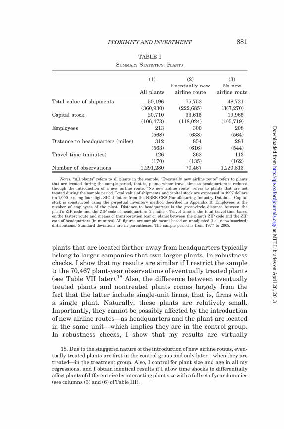
plants that are located farther away from headquarters typicallybelong to larger companies that own larger plants. In robustnesschecks, I show that my results are similar if I restrict the sampleto the 70,467 plant-year observations of eventually treated plants(see Table VII later).18 Also, the difference between eventuallytreated plants and nontreated plants comes largely from thefact that the latter include single-unit firms, that is, firms witha single plant. Naturally, these plants are relatively small.Importantly, they cannot be possibly affected by the introductionof new airline routes—as headquarters and the plant are locatedin the same unit—which implies they are in the control group.In robustness checks, I show that my results are virtually

TABLE I

SUMMARY STATISTICS: PLANTS

(1) (2) (3)

All plantsEventually new

airline routeNo new

airline route

Total value of shipments 50,196 75,752 48,721(360,930) (222,685) (367,270)

Capital stock 20,710 33,615 19,965(106,473) (118,024) (105,719)

Employees 213 300 208(568) (638) (564)

Distance to headquarters (miles) 312 854 281(563) (616) (544)

Travel time (minutes) 126 362 113(170) (135) (162)

Number of observations 1,291,280 70,467 1,220,813

Notes. ‘‘All plants’’ refers to all plants in the sample. ‘‘Eventually new airline route’’ refers to plantsthat are treated during the sample period, that is, plants whose travel time to headquarters is reducedthrough the introduction of a new airline route. ‘‘No new airline route’’ refers to plants that are nottreated during the sample period. Total value of shipments and capital stock are expressed in 1997 dollars(in 1,000 s) using four-digit SIC deflators from the NBER-CES Manufacturing Industry Database. Capitalstock is constructed using the perpetual inventory method described in Appendix B. Employees is thenumber of employees of the plant. Distance to headquarters is the great-circle distance between theplant’s ZIP code and the ZIP code of headquarters (in miles). Travel time is the total travel time basedon the fastest route and means of transportation (car or plane) between the plant’s ZIP code and the ZIPcode of headquarters (in minutes). All figures are sample means based on unadjusted (i.e., nonwinsorized)distributions. Standard deviations are in parentheses. The sample period is from 1977 to 2005.

18. Due to the staggered nature of the introduction of new airline routes, even-tually treated plants are first in the control group and only later—when they aretreated—in the treatment group. Also, I control for plant size and age in all myregressions, and I obtain identical results if I allow time shocks to differentiallyaffect plants of different size by interacting plant size with a full set of year dummies(see columns (3) and (6) of Table III).


at MIT

Libraries on A


Dow

nloaded from


unchanged if I exclude single-unit firms from the sample (seeTable VII later).

The 70,467 plant-year observations in column (2) of Table Icorrespond to 10,533 treated plants.19 In Table II, I provide aux-iliary information about the nature of the treatments. New air-line routes can be classified into four categories: (1) ‘‘Direct toDirect’’: a new direct flight using a different route replaces a pre-viously optimal direct flight, for example, the new flight involvesan airport that is closer to either headquarters or the plant; (2)‘‘Indirect to Indirect’’: a new indirect flight using a different routereplaces a previously optimal indirect flight, for example, the newindirect flight has only one stopover, while the previously optimalindirect flight had two stopovers; (3) ‘‘Indirect to Direct’’: a newdirect flight replaces a previously optimal indirect flight, for ex-ample, as in the Boston-Memphis example; (4) ‘‘Road to Flight’’: anew direct or indirect flight replaces car travel as the previouslyoptimal means of transportation.20

For all treated plants (column (1)) and separately also foreach of the above four categories (columns (2)–(5)), Table II re-ports the average distance (in miles) between headquarters andplants, the average travel time before and after the introductionof the new airline routes, and the average reduction in traveltime, both in absolute and relative terms. As column (1) shows,the average travel time reduction across all treated plants is 1hour, 43 minutes for a one-way trip, which amounts to a traveltime reduction of 25%. The breakdown in columns (2) to (5) showsthat the category ‘‘Indirect to Indirect’’ accounts for the largestreduction in travel time (2 hours, 26 minutes), followed by thecategory ‘‘Indirect to Direct’’ (2 hours, 7 minutes) and the cat-egory ‘‘Direct to Direct’’ (1 hour, 12 minutes). Also, as onewould expect, larger travel time reductions are associated with

19. Thus, on average, I have about seven years of data for each treated plant. Ihave verified that my results are robust if I only include plants for which I have datafor the entire 10-year treatment window.

20. To give an example of a ‘‘Direct to Direct’’ treatment, suppose a firm head-quartered in Atlanta has a plant in Naples, FL. In 1982, the fastest way to travelfrom Atlanta to Naples was to take a direct flight from ATL to FLL (Fort LauderdaleInternational Airport) and then to drive to Naples. In 1983, Delta Airlines startedoperating direct flights between ATL and RSW (Southwest Florida InternationalAirport), which is located right next to Naples. Thus, in this case, a previouslyoptimal direct flight (ATL to FLL) is replaced by a new, and faster, direct flight(ATL to RSW).


at MIT

Libraries on A


Dow

nloaded from


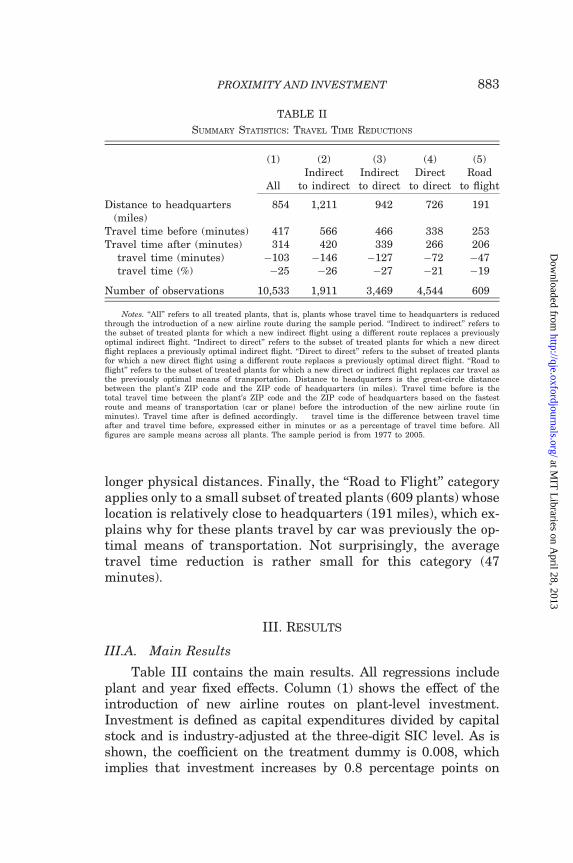
longer physical distances. Finally, the ‘‘Road to Flight’’ categoryapplies only to a small subset of treated plants (609 plants) whoselocation is relatively close to headquarters (191 miles), which ex-plains why for these plants travel by car was previously the op-timal means of transportation. Not surprisingly, the averagetravel time reduction is rather small for this category (47minutes).

III. Results

III.A. Main Results

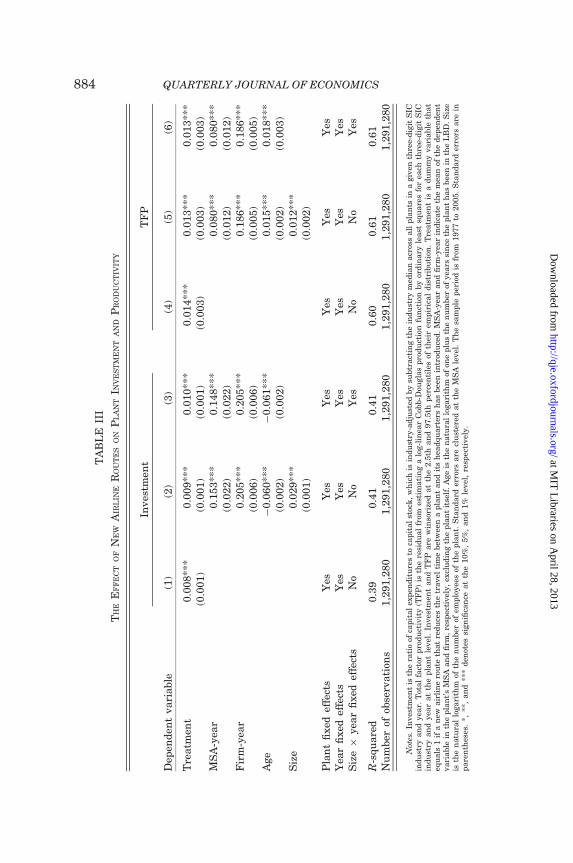
Table III contains the main results. All regressions includeplant and year fixed effects. Column (1) shows the effect of theintroduction of new airline routes on plant-level investment.Investment is defined as capital expenditures divided by capitalstock and is industry-adjusted at the three-digit SIC level. As isshown, the coefficient on the treatment dummy is 0.008, whichimplies that investment increases by 0.8 percentage points on

TABLE II

SUMMARY STATISTICS: TRAVEL TIME REDUCTIONS

(1) (2) (3) (4) (5)

AllIndirect

to indirectIndirectto direct

Directto direct

Roadto flight

Distance to headquarters(miles)

854 1,211 942 726 191

Travel time before (minutes) 417 566 466 338 253Travel time after (minutes) 314 420 339 266 206� travel time (minutes) �103 �146 �127 �72 �47� travel time (%) �25 �26 �27 �21 �19

Number of observations 10,533 1,911 3,469 4,544 609

Notes. ‘‘All’’ refers to all treated plants, that is, plants whose travel time to headquarters is reducedthrough the introduction of a new airline route during the sample period. ‘‘Indirect to indirect’’ refers tothe subset of treated plants for which a new indirect flight using a different route replaces a previouslyoptimal indirect flight. ‘‘Indirect to direct’’ refers to the subset of treated plants for which a new directflight replaces a previously optimal indirect flight. ‘‘Direct to direct’’ refers to the subset of treated plantsfor which a new direct flight using a different route replaces a previously optimal direct flight. ‘‘Road toflight’’ refers to the subset of treated plants for which a new direct or indirect flight replaces car travel asthe previously optimal means of transportation. Distance to headquarters is the great-circle distancebetween the plant’s ZIP code and the ZIP code of headquarters (in miles). Travel time before is thetotal travel time between the plant’s ZIP code and the ZIP code of headquarters based on the fastestroute and means of transportation (car or plane) before the introduction of the new airline route (inminutes). Travel time after is defined accordingly. � travel time is the difference between travel timeafter and travel time before, expressed either in minutes or as a percentage of travel time before. Allfigures are sample means across all plants. The sample period is from 1977 to 2005.


at MIT

Libraries on A


Dow

nloaded from


TA

BL

EII

I

TH

EE

FF

EC

TO

FN

EW

AIR

LIN

ER

OU

TE

SO

NP

LA

NT

INV

ES

TM

EN

TA

ND

PR

OD

UC

TIV

ITY

Dep

end

ent

vari

able

Inves

tmen

tT

FP

(1)

(2)

(3)

(4)

(5)

(6)

Tre

atm

ent

0.0

08**

*0.0

09**

*0.0

10**

*0.0

14**

*0.0

13**

*0.0

13**

*(0

.001)

(0.0

01)

(0.0

01)

(0.0

03)

(0.0

03)

(0.0

03)

MS

A-y

ear

0.1

53**

*0.1

48**

*0.0

80**

*0.0

80**

*(0

.022)

(0.0

22)

(0.0

12)

(0.0

12)

Fir

m-y

ear

0.2

05**

*0.2

05**

*0.1

86**

*0.1

86**

*(0

.006)

(0.0

06)

(0.0

05)

(0.0

05)

Age

�0.0

60**

*�

0.0

61**

*0.0

15**

*0.0

18**

*(0

.002)

(0.0

02)

(0.0

02)

(0.0

03)

Siz

e0.0

29**

*0.0

12**

*(0

.001)

(0.0

02)

Pla

nt

fixed

effe

cts

Yes

Yes

Yes

Yes

Yes

Yes

Yea

rfi

xed

effe

cts

Yes

Yes

Yes

Yes

Yes

Yes

Siz

e�

yea

rfi

xed

effe

cts

No

No

Yes

No

No

Yes

R-s

qu

are

d0.3

90.4

10.4

10.6

00.6

10.6

1N

um

ber

ofob

serv

ati

ons

1,2

91,2

80

1,2

91,2

80

1,2

91,2

80

1,2

91,2

80

1,2

91,2

80

1,2

91,2

80

Not

es.

Inves

tmen

tis

the

rati

oof

cap

ital

exp

end

itu

res

toca

pit

al

stoc

k,

wh

ich

isin

du

stry

-ad

just

edby

subtr

act

ing

the

ind

ust

rym

edia

nacr

oss

all

pla

nts

ina

giv

enth

ree-

dig

itS

ICin

du

stry

an

dyea

r.T

otal

fact

orp

rod

uct

ivit

y(T

FP

)is

the

resi

du

al

from

esti

mati

ng

alo

g-l

inea

rC

obb-D

ougla

sp

rod

uct

ion

fun

ctio

nby

ord

inary

least

squ

are

sfo

rea

chth

ree-

dig

itS

ICin

du

stry

an

dyea

rat

the

pla

nt

level

.In

ves

tmen

tan

dT

FP

are

win

sori

zed

at

the

2.5

than

d97.5

thp

erce

nti

les

ofth

eir

emp

iric

al

dis

trib

uti

on.

Tre

atm

ent

isa

du

mm

yvari

able

that

equ

als

1if

an

ewair

lin

ero

ute

that

red

uce

sth

etr

avel

tim

ebet

wee

na

pla

nt

an

dit

sh

ead

qu

art

ers

has

bee

nin

trod

uce

d.

MS

A-y

ear

an

dfi

rm-y

ear

ind

icate

the

mea

nof

the

dep

end

ent

vari

able

inth

ep

lan

t’s

MS

Aan

dfi

rm,

resp

ecti

vel

y,

excl

ud

ing

the

pla

nt

itse

lf.

Age

isth

en

atu

ral

logari

thm

ofon

ep

lus

the

nu

mber

ofyea

rssi

nce

the

pla

nt

has

bee

nin

the

LB

D.

Siz

eis

the

natu

ral

logari

thm

ofth

en

um

ber

ofem

plo

yee

sof

the

pla

nt.

Sta

nd

ard

erro

rsare

clu

ster

edat

the

MS

Ale

vel

.T

he

sam

ple

per

iod

isfr

om1977

to2005.

Sta

nd

ard

erro

rsare

inp

are

nth

eses

.*,

**,

an

d**

*d

enot

essi

gn

ifica

nce

at

the

10%

,5%

,an

d1%

level

,re

spec

tivel

y.


at MIT

Libraries on A


Dow

nloaded from


average. The coefficient is statistically highly significant. It is alsoeconomically significant. Given that the sample mean of plant-levelinvestment is 0.10, an increase of 0.8 percentage points impliesthat investment increases by 8%, corresponding to an increase incapital expenditures of $158,000 (in 1997 dollars).21

In column (2), I account for the possibility of local shocks(by including MSA-year controls) and shocks at the firm level(by including firm-year controls). The MSA- and firm-year con-trols are described in Section II.B. I also control for plant age andsize. Age is the logarithm of one plus the number of years sincethe plant has been covered in the LBD. Size is the logarithm of thenumber of employees. As shown, the results are not sensitive tothe inclusion of controls. If anything, the coefficient on thetreatment dummy becomes slightly larger: the coefficient is now0.009, which implies that plant-level investment increases by 9%,corresponding to an increase in capital expenditures of $177,000(in 1997 dollars). In column (3), I allow time shocks to differen-tially affect plants of different size by interacting plant size with afull set of year dummies. Again, this has little impact on myresults.

In columns (4) to (6), I reestimate the specifications in col-umns (1) to (3) with TFP as the dependent variable. TFP isdefined in Section II.C. Recall that TFP measures the relativeproductivity of a plant within an industry. The coefficient onthe treatment dummy is between 0.013 and 0.014, which impliesTFP increases by 1.3% to 1.4%, respectively, corresponding to anincrease in profits (in 1997 dollars) of $275,000 and $296,000,respectively.22

21. A coefficientof 0.008 implies an increase in capital expenditures equal to 0.8%of capital stock. Given that the average capital stock of treated plants is $19.7 mil-lion—based on the winsorized distribution of capital stock, consistent with the wayinvestment is constructed (see Section II.C)—this implies an increase in plant-levelcapital expenditures of 0.008�$19.7 million = $158,000.

22. A 1.3% increase in TFP implies, by definition, that the plant produces a 1.3%higher value of shipments with exactly the same inputs. Accordingly, the increase inplant-level profits can be approximated by multiplying the pretreatment averagevalue of shipments of treated plants based on the winsorized distribution (consistentwith the way TFP is constructed, see Section II.C) by 0.013. This pretreatment aver-age is$32.5 million, implying an increase in plant-level profits of 0.65�0.013�$32.5million = $275,000 (using a corporate tax rate of 35%). This figure is likely an over-statement, however, as it only accounts for expenses incurred by the plant but not forthose incurred by headquarters (e.g., travel costs and other headquarters-relatedexpenses that may arise following the treatment).


at MIT

Libraries on A


Dow

nloaded from


In the remainder of this article, I use the specification incolumns (2) and (5)—which includes MSA- and firm-year con-trols, plant age, and plant size—as my baseline specification.All my results are similar if I exclude these four controls, if Iinclude only a subset, or if I additionally control for firm ageand firm size.

III.B. Dynamic Effects of New Airline Routes

As discussed in Section II.B, an important concern is thatomitted plant-specific shocks could be driving both the introduc-tion of new airline routes and plant-level investment or product-ivity. Because these shocks do not affect other plants in the sameregion, they cannot be accounted for by the inclusion of MSA-yearcontrols. Likewise, as they do not affect other plants of the samefirm, they cannot be accounted for by the inclusion of firm-yearcontrols.

If a new airline route is the (endogenous) outcome of a pre-existing plant-specific shock, then I should find an ‘‘effect’’ of thetreatment already before the new airline route is introduced. Toinvestigate this issue, I study in detail the dynamic effects of theintroduction of new airline routes. Given that annual records inthe CMF and ASM are measured in calendar years, the lastmonth of each plant-year observation is December. Because theT-100 and ER-586 segment data are at monthly frequency, thismeans I know precisely in which month a new airline route isintroduced. Accordingly, I am able to reconstruct how manymonths before or after the introduction of a new airline route agiven plant-year observation is recorded. For instance, consideragain the Boston-Memphis example. In this example, the 1985plant-year observation of the Memphis plant is recorded 9months before the treatment; the 1986 plant-year observation isrecorded 3 months after the treatment; the 1987 plant-year ob-servation is recorded 15 months after the treatment, and so on.

By exploiting the detailed knowledge of the months in whichnew airline routes are introduced, I can replace the treatmentdummy in equation (1) with a set of dummies indicating thetime interval between a given plant-year observation andthe treatment. I use eight dummies. The first dummy,‘‘Treatment (�12 m,�6 m),’’ equals 1 if the plant-year observationis recorded between 12 and 6 months before the treatment. Theother dummies are defined accordingly with respect to the


at MIT

Libraries on A


Dow

nloaded from


intervals (�6 m, 0 m), (0 m, 6 m), (6 m, 12 m), (12 m, 18 m), (18 m,24 m), (24 m, 30 m), and 30 months and beyond (‘‘30 m +’’).

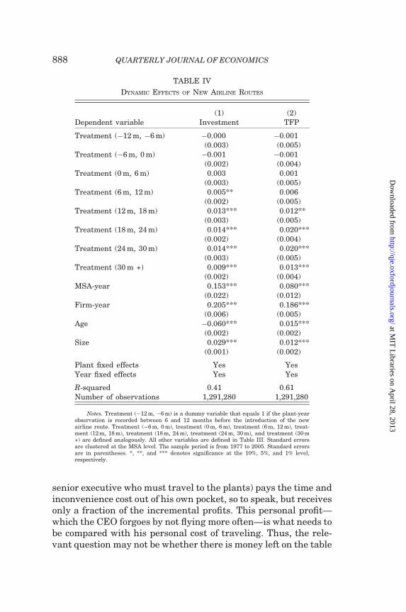
Table IV shows the results. In column (1), the dependentvariable is plant-level investment. The main variables of interestare Treatment (�12 m, �6 m) and Treatment (�6 m, 0 m), whichmeasure the ‘‘effect’’ of the new airline routes before their intro-duction. As is shown, the coefficients on both variables are smalland insignificant, which suggests that there are no pre-existingtrends in the data. Interestingly, the coefficient on Treatment(0 m, 6 m), which captures the effect of the new airline routeswithin the first six months after their introduction, is also insig-nificant. Moreover, although the effect becomes significant aftersix months, it remains initially small in economic terms. It is onlyafter 12 months that the effect becomes large and highly signifi-cant. Precisely, the coefficients on Treatment (12 m, 18 m),Treatment (18 m, 24 m), and Treatment (24 m, 30 m) are between0.013 and 0.014, which implies that plant-level investment in-creases by 13% to 14%. In the longer run—that is 30 monthsand beyond—the magnitude of the coefficient reverts to a slightlylower level. In column (2), the dependent variable is TFP. Thepattern is similar to above, except that the increase in TFP occurssix months after the increase in investment. Accordingly, theeffect on TFP becomes significant only after 12 months, and itbecomes economically large only after 18 months.

III.C. Discussion

Money Left on the Table? My results suggest that plant-levelprofits increase by $275,000 to $296,000 on average (see SectionIII.A). This raises the question of whether there is or, precisely,was ‘‘money left on the table.’’ In particular, if the increase inprofits is so large, why did the CEO (or some other seniorexecutive) not already fly more often to the plants before? Oneanswer is that the CEO is so time-constrained that, absent a re-duction in travel time, he was simply unable to travel more often.Consistent with this argument, I document in Section V.A thatthe treatment effect is stronger for firms whose managers aremore time-constrained.

Another way of looking at the magnitudes of my estimates isfrom an agency perspective.23 Indeed, the CEO (or some other

23. I am very grateful to the editor, Andrei Shleifer, for suggesting thisargument.


at MIT

Libraries on A


Dow

nloaded from


senior executive who must travel to the plants) pays the time andinconvenience cost out of his own pocket, so to speak, but receivesonly a fraction of the incremental profits. This personal profit—which the CEO forgoes by not flying more often—is what needs tobe compared with his personal cost of traveling. Thus, the rele-vant question may not be whether there is money left on the table

TABLE IV

DYNAMIC EFFECTS OF NEW AIRLINE ROUTES

(1) (2)Dependent variable Investment TFP

Treatment (�12 m, �6 m) �0.000 �0.001(0.003) (0.005)

Treatment (�6 m, 0 m) �0.001 �0.001(0.002) (0.004)

Treatment (0 m, 6 m) 0.003 0.001(0.003) (0.005)

Treatment (6 m, 12 m) 0.005** 0.006(0.002) (0.005)

Treatment (12 m, 18 m) 0.013*** 0.012**(0.003) (0.005)

Treatment (18 m, 24 m) 0.014*** 0.020***(0.002) (0.004)

Treatment (24 m, 30 m) 0.014*** 0.020***(0.003) (0.005)

Treatment (30 m +) 0.009*** 0.013***(0.002) (0.004)

MSA-year 0.153*** 0.080***(0.022) (0.012)

Firm-year 0.205*** 0.186***(0.006) (0.005)

Age �0.060*** 0.015***(0.002) (0.002)

Size 0.029*** 0.012***(0.001) (0.002)

Plant fixed effects Yes YesYear fixed effects Yes Yes

R-squared 0.41 0.61Number of observations 1,291,280 1,291,280

Notes. Treatment (�12 m, �6 m) is a dummy variable that equals 1 if the plant-yearobservation is recorded between 6 and 12 months before the introduction of the newairline route. Treatment (�6 m, 0 m), treatment (0 m, 6 m), treatment (6 m, 12 m), treat-ment (12 m, 18 m), treatment (18 m, 24 m), treatment (24 m, 30 m), and treatment (30 m+) are defined analogously. All other variables are defined in Table III. Standard errorsare clustered at the MSA level. The sample period is from 1977 to 2005. Standard errorsare in parentheses. *, **, and *** denotes significance at the 10%, 5%, and 1% level,respectively.


at MIT

Libraries on A


Dow

nloaded from


for the firm, but rather whether there is money left on the tablefor the CEO himself.

To estimate the CEO’s personal profits, I merge my samplewith ExecuComp, which contains detailed information on execu-tive compensation, including CEO ownership. Alas, merging mysample with ExecuComp significantly reduces the number of ob-servations, first, because ExecuComp includes only large, pub-licly traded firms and, second, because ExecuComp begins onlyin 1992. I compute CEO ownership in two ways. First, I computethe ratio of shares held by the CEO to the total number of sharesoutstanding. This measure ignores stock options and may there-fore underestimate CEO ownership. To mitigate this concern, Ialso compute the ratio of shares and option deltas held by theCEO to the total number of shares and option deltas outstanding.Stock option deltas are computed using the methodology in Coreand Guay (2002). Depending on which measure I use, I find thatthe average pretreatment CEO ownership is between 1.3% and1.4%.

I then reestimate my baseline TFP regression using theExecuComp subsample. I find that the coefficient on the treat-ment dummy is 0.010, which corresponds to an increase inplant-level profits of $312,000. (This is slightly higher than theprofit increase of $275,000 to $296,000 reported in Section III.A,because the plants of companies included in ExecuComp are onaverage larger than those in my main sample.) Given that CEOownership is between 1.3% and 1.4%, this implies an increase inthe CEO’s personal profits of $4,056 to $4,368.24 Although this isof course speculative, I find it plausible to think of this personalprofit as being relatively small from a (wealthy) CEO’s perspec-tive—possibly small enough that it does not compensate him forhis personal time and inconvenience cost.

Maybe the CEO would have been more likely to travel if thefirm had a corporate jet. Though entry-level jets are available fora couple of million dollars (with top-of-the-line models costing $30million and more), the annual operating costs are substantial. Forinstance, Edgerton (2012, 2188) estimates that ‘‘annual operating

24. This is likely an overstatement of a CEO’s personal profits. As plant-levelprofits do not include expenses incurred by headquarters, for example, overheadand travel expenses, the increase in firm-level profits is likely to be less than$312,000, which implies that the increase in the CEO’s personal profits is lessthan $4,056 to $4,368.


at MIT

Libraries on A


Dow

nloaded from


costs can be as high as $5 million per jet, with $1 million beingquite typical.’’ Also, fractional ownership of jets, an innovationthat significantly reduced the costs of using private jets, hasbecome available only relatively late during my sampleperiod.25 Leaving cost considerations aside, there may also beother reasons firms do not use corporate jets. One such reasonmay be corporate governance, given that private jets may be ex-cessively used for the pursuit of private benefits. Consistent withthis picture, Edgerton (2012) finds that firms undergoing lever-aged buyouts significantly reduce their fleet of corporate jets.Also, Yermack (2006) finds that the use of corporate jets is sig-nificantly related to CEOs’ long-distance golf club memberships,and that companies allowing personal aircraft use by their CEOunderperform market benchmarks by about 4% per year.26

Maybe it would pay the firm to hire ‘‘delegated monitors’’ anddeploy them at the plant? Again, it is unclear whether a profitincrease of $275,000 to $296,000 is enough to justify the costs.More important, it is unclear whether delegated monitorswould be an effective substitute for the CEO or some othersenior manager visiting the plant. Indeed, the very definitionof soft information argues that it ‘‘cannot be crediblytransmitted’’ (Stein 2002, 1891) and ‘‘cannot be directly verifiedby anyone other than the agent who produces it’’ (1892).Consequently, to the extent that capital budgeting decisions are(partly) based on soft information, there is no effective substitutefor the CEO (or whoever makes the decision) personally visitingthe plant.

Spillover Effects. That plant-level TFP increases does notautomatically imply that the company is better off. Maybe the

25. In 1986, NetJets pioneered the concept of fractional ownership of privatejets, but it has become widely popular only since the mid-1990s (National BusinessAviation Administration 2004). Nevertheless, the increased use of private jets sincethe mid-1990s may be an alternative explanation—in addition to the one given inSection V.B—for why the treatment effect has become significantly weaker duringthe later years of my sample period (see Table IX for details).

26. See also ‘‘Corporate Jet Set: Leisure vs. Business’’ (Wall Street Journal,June 16, 2011), reporting that, for some companies, more than half of all flightsgo to resort areas such as Palm Beach, Aspen, or the Bahamas.


at MIT

Libraries on A


Dow

nloaded from


CEO or other managers—who can now travel more easily to theplant—do not really add any monitoring value at all, but theythink they do. If so, they might draw comfort from their addedinvolvement and invest more in the plant. This might make theplant more productive (i.e., TFP increases), especially if the plantwas below the first-best level of investment before, for example,because the firm is financially constrained. However, under thisalternative scenario, the rest of the firm would probably suffer,because all that is going on is an inefficient reallocation of capitalbased on a mistake. Likewise, if the reduction in travel timemakes it easier for plant-level managers to lobby headquarters,investment and productivity at the treated plant might increase(at the expense of other plants). However, if all that is going on isan inefficient reallocation based on lobbying, overall productivity(at the firm level) should not increase. In fact, it should probablydecline.

In follow-up work, I take a closer look at such spillover effects(Giroud and Mueller 2012). The research is motivated by the factthat theory on internal capital markets predicts that—providedfirms are financially constrained—positive shocks to investmentat one plant should lead to a decline in investment at other plants(e.g., Stein 1997). However, if the reallocation is overall efficient,firm-level productivity should rise. The main results are as fol-lows. On average, there are no spillovers to other plants. Thus, onaverage, the increase in investment and productivity at the trea-ted plant documented here is indeed a ‘‘net effect,’’ which trans-lates into higher investment and productivity for the firm as awhole. That being said, when we look separately at financiallyconstrained and unconstrained firms, we find evidence of nega-tive spillovers among financially constrained firms—that is,investment at other plants declines. In contrast, we find no evi-dence of spillovers at financially unconstrained firms. However,even in situations where spillovers exist, overall firm-level prod-uctivity improves, suggesting that the resource reallocation isbeneficial for the firm as a whole.

IV. Robustness

Not finding a significant treatment effect either before orimmediately after the introduction of new airline routes (seeTable IV) mitigates concerns that my results are driven by


at MIT

Libraries on A


Dow

nloaded from


preexisting plant-specific shocks. However, it could still be that anew airline route is introduced in anticipation of a futureplant-specific shock. Or it could be that the shock leads first tothe introduction of a new airline route and only later to an in-crease in plant-level investment (productivity). Both interpret-ations are consistent with the absence of preexisting trends.More generally, any shock whose dimension is at theplant-headquarters level is a potential remaining concern. Assuch shocks are collinear with the treatment, they cannot be fil-tered out by the inclusion of MSA- or firm-year controls. Thisincludes, for example, the possibility of pair-specific shocks totrade between the plant’s and headquarters’ locations, in thesense that only plants in location A with headquarters in locationB—but not plants in location A in general—are affected by theshock. The robustness tests in this section are meant to addressthis remaining concern.

IV.A. Hub Openings and Airline Mergers

In this section, I show that my results are robust when Iconsider only new airline routes that are the outcome of amerger between two airlines or the opening of a new hub.27

Arguably, it is rather unlikely that a shock to a single plant—ora pair-specific shock that affects only plants in location A withheadquarters in location B—would be responsible for an airlinemerger or a hub opening.

Table A.1 in the Online Appendix provides a list of airlinehubs that were opened during the sample period. The list is com-piled from two sources: newspaper reports and airlines’ annualreports. The newspaper reports are obtained from various news-paper databases (ProQuest, Factiva, and Newsbank America’sNewspapers). Precisely, I ran a search for articles that containthe airline name, the airport name, and the word ‘‘hub.’’ Thesearticles are supplemented with information about hub openingsthat airlines self-report in their annual reports. As can be seen,most of the hub openings date back to the 1980s. In the yearsfollowing the Airline Deregulation Act of October 1978, airlinesstarted competing for strategic hub locations, and as a result,the 1980s witnessed a substantial number of new hub openings(Ivy 1993).

27. I thank Adair Morse for suggesting the idea to look at hub openings.


at MIT

Libraries on A


Dow

nloaded from




Table A.2 in the Online Appendix provides a list of airlinemergers that were completed during the sample period.28 The listis compiled from the same sources as the list of hub openings andis supplemented with merger information from Thompson’sSecurities Data Corporation (SDC) database. Although many air-line mergers were completed during the sample period, I consideronly mergers that account for at least one treatment in mysample. Mergers of small commuter airlines servicing few loca-tions often do not satisfy this criterion.29 As is shown in Table A.2,the pattern of airline mergers mirrors that of new hub openings.The increase in competition induced by the Airline DeregulationAct of 1978 forced many airlines to file for bankruptcy or mergewith another airline. By 1990, this consolidation phase was lar-gely completed. As a result, industry-wide concentration hadincreased sharply, with the nine largest airlines representing atotal market share of over 90% of domestic revenue passengermiles (Goetz and Sutton 1997).

28. Airline mergers can lead to both the introduction of new airline routes andthe termination of existing routes. New airline routes are typically introduced asthe acquirer airline takes over the gates of the target airline at airports that werepreviously not serviced by the acquirer. For instance, in 1986, American Airlinesacquired Air California (AirCal), a regional carrier operating in California. AirCalhad previously serviced regional airports such as Sacramento, Palm Springs, andOakland. After taking over AirCal’s gates at these airports, American Airlinesintroduced several new airline routes, for example, from Chicago to Sacramentoor from Nashville to Oakland. Route terminations are examined separately inSection IV.C.

29. I apply three additional criteria when compiling the list of airline mergers.First, I consider only mergers that resulted in an actual merger of the airlines’operations. For example, Southwest Airlines acquired Muse Air in 1985 and oper-ated it as a fully owned subsidiary until its liquidation in 1987. Since an integrationof the Muse Air routes into the Southwest network never occurred, I do not code thisevent as a merger. Second, the year of the merger in Table A.2 is the year in whichthe airlines actually merged their operations, not the year in which the merger wasconsummated. For example, Delta Airlines acquired Western Airlines on December16, 1986. For a few months, Western was operated as a fully owned subsidiary. It isonly several months later, on April 1, 1987, that Western’s operations were mergedinto the Delta network. Hence, in Table A.2, the relevant merger year is 1987.Third, in two cases, the term ‘‘Acquirer Airline’’ refers to the name of the mergedentity, not the actual acquirer. In the 1997 merger of AirTran Airways and ValueJetAirlines, the acquirer was actually ValueJet. However, the merged carrier retainedthe AirTran name, brand, and identity. Likewise, in the 1982 merger of ContinentalAirlines and Texas International Airlines, the acquirer was Texas Air (the owner ofTexas International Airlines). The merged airline retained the Continental name,however.


at MIT

Libraries on A


Dow

nloaded from







Based on the list of hub openings and airline mergers, Idivide the 10,533 treated plants into three categories: ‘‘hub treat-ments,’’ ‘‘merger treatments,’’ and ‘‘other treatments.’’ Hub treat-ments involve new airline routes that are introduced by airlinesin the same year as they open a new hub. Merger treatments aredefined analogously with respect to airline mergers.30 In total, mysample includes 1,761 hub treatments and 535 merger treat-ments, which together account for 22% of all treated plants.This high percentage indicates that hub openings and airlinemergers are significant events in the lives of airlines.

Figure I provides additional statistics. The diamond dotsmark the number of newly treated plants (‘‘treatments’’) peryear where the treatment involves a new airline route that isintroduced by an airline that opens a new hub in year zero(event year). All years (i.e., –2, –1, etc.) are measured relative tothe event year. As shown, the number of new treatments invol-ving airlines that open a new hub is roughly constant in the yearsbefore and after the hub opening. However, in the year of the hubopening, the number of new treatments is about three timeshigher. I obtain a similar pattern when I consider new treatmentsinvolving airlines that merge in year zero (marked by square dotsin Figure I).31 In either case, the spike in the event year confirmsthat airlines substantially expand their route networks whenopening a new hub or integrating other airlines’ routes intotheir own operations.

In Table V, I replace the treatment dummy in equation (1)with a set of three dummies indicating whether the treatment is ahub treatment, merger treatment, or other treatment. As shown,the coefficients on all three dummies are statistically significantand economically large. The coefficient is largest for hub treat-ments, slightly smaller for merger treatments, and smallestfor the other treatments. The differences among the coefficientsare likely reflective of the fact that new airline routes thatare introduced as part of a hub opening or airline merger aremostly long-distance routes, which tend to be associated withlarger travel time reductions. As I show in robustness checks

30. If a merger treatment coincides with a hub treatment, I classify the event asa hub treatment. For instance, in 1987, Delta Airlines merged the operations ofWestern Airlines into their network and opened a new hub in Salt Lake City on thebasis of the former Western hub.

31. In the years preceding the merger, the number of new treatments per yearincludes treatments associated with both the acquirer and target airlines.


at MIT

Libraries on A


Dow

nloaded from


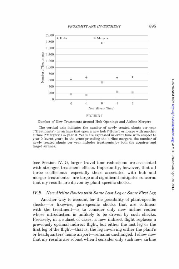
(see Section IV.D), larger travel time reductions are associatedwith stronger treatment effects. Importantly, however, that allthree coefficients—especially those associated with hub andmerger treatments—are large and significant mitigates concernsthat my results are driven by plant-specific shocks.

IV.B. New Airline Routes with Same Last Leg or Same First Leg

Another way to account for the possibility of plant-specificshocks—or likewise, pair-specific shocks that are collinearwith the treatment—is to consider only new airline routeswhose introduction is unlikely to be driven by such shocks.Precisely, in a subset of cases, a new indirect flight replaces apreviously optimal indirect flight, but either the last leg or thefirst leg of the flight—that is, the leg involving either the plant’sor headquarters’ home airport—remains unchanged. I show nowthat my results are robust when I consider only such new airline

0

200

400

600

800

1,000

1,200

1,400

1,600

1,800

2,000

-2 -1 0 1 2

Num

ber o

f Tre

atm

ents

Year (Event Time)

Hubs Mergers

FIGURE I

Number of New Treatments around Hub Openings and Airline Mergers

The vertical axis indicates the number of newly treated plants per year(‘‘Treatments’’) by airlines that open a new hub (‘‘Hubs’’) or merge with anotherairline (‘‘Mergers’’) in year 0. Years are expressed in event time with respect toyear 0 (event year). In the years preceding the airline mergers, the number ofnewly treated plants per year includes treatments by both the acquirer andtarget airlines.


at MIT

Libraries on A


Dow

nloaded from


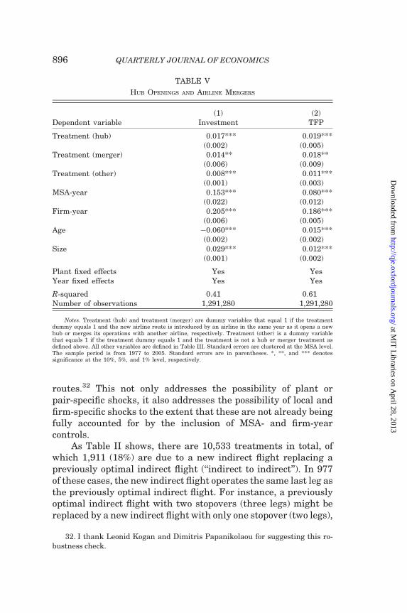
routes.32 This not only addresses the possibility of plant orpair-specific shocks, it also addresses the possibility of local andfirm-specific shocks to the extent that these are not already beingfully accounted for by the inclusion of MSA- and firm-yearcontrols.

As Table II shows, there are 10,533 treatments in total, ofwhich 1,911 (18%) are due to a new indirect flight replacing apreviously optimal indirect flight (‘‘indirect to indirect’’). In 977of these cases, the new indirect flight operates the same last leg asthe previously optimal indirect flight. For instance, a previouslyoptimal indirect flight with two stopovers (three legs) might bereplaced by a new indirect flight with only one stopover (two legs),

TABLE V

HUB OPENINGS AND AIRLINE MERGERS


Treatment (hub) 0.017*** 0.019***(0.002) (0.005)

Treatment (merger) 0.014** 0.018**(0.006) (0.009)

Treatment (other) 0.008*** 0.011***(0.001) (0.003)

MSA-year 0.153*** 0.080***(0.022) (0.012)

Firm-year 0.205*** 0.186***(0.006) (0.005)

Age �0.060*** 0.015***(0.002) (0.002)

Size 0.029*** 0.012***(0.001) (0.002)



Notes. Treatment (hub) and treatment (merger) are dummy variables that equal 1 if the treatmentdummy equals 1 and the new airline route is introduced by an airline in the same year as it opens a newhub or merges its operations with another airline, respectively. Treatment (other) is a dummy variablethat equals 1 if the treatment dummy equals 1 and the treatment is not a hub or merger treatment asdefined above. All other variables are defined in Table III. Standard errors are clustered at the MSA level.The sample period is from 1977 to 2005. Standard errors are in parentheses. *, **, and *** denotessignificance at the 10%, 5%, and 1% level, respectively.

32. I thank Leonid Kogan and Dimitris Papanikolaou for suggesting this ro-bustness check.


at MIT

Libraries on A


Dow

nloaded from


but the last leg of the flight—that is, the leg connecting the plant’shome airport—remains unchanged (see the BOS-ATL-MEM-LITexample in Section II.B). Because the last leg of the flight is un-changed, it is rather unlikely that this new airline route wastriggered by a plant-specific shock or local shock in the plant’svicinity. In the remaining 934 cases, the new indirect flight oper-ates the same first leg as the previously optimal indirect flight.(Hence, there exists no ‘‘indirect to indirect’’ treatment whereeither both the last and first leg have changed or where bothlegs remain unchanged.) By the same token as above, giventhat the first leg of the flight—the leg connecting headquarters’home airport—remains unchanged, it is rather unlikely that thisnew airline route was triggered by a shock at the firm level.

In Table VI, I replace the treatment dummy in equation (1)with a set of three dummies indicating whether the treatment isdue to a new indirect flight operating the same last leg (‘‘same lastleg’’), a new indirect flight operating the same first leg (‘‘same firstleg’’), or any other new flight (‘‘other’’). As shown, the coefficientson all three dummies are statistically significant and economic-ally large. The coefficient is largest for the ‘‘same first leg’’ and‘‘same last leg’’ treatments, which is reflective of the fact that‘‘indirect to indirect’’ treatments, are associated with largertravel time reductions (see Table II). Importantly, however, thefact that all three coefficients—especially those associated withthe ‘‘same first leg’’ and ‘‘same last leg’’ treatments—are large andsignificant alleviates concerns that my findings are driven byplant- or pair-specific shocks, local shocks, or shocks at the firmlevel.

IV.C. Alternative Control Groups

In my baseline specification, the control group consists of allplants that have not (yet) been treated. Due to the staggerednature of the introduction of new airline routes, this includesplants that are never treated during the sample period as wellas plants that will be treated at some future time. In this section, Iexamine the robustness of my results to using alternative controlgroups. The results are presented in Table VII.

Multiunit Firms. In columns (1) and (2), I exclude single-unitfirms from the sample, which means the sample consists exclu-sively of multiunit firms. As explained in Section II.D, single-unit


at MIT

Libraries on A


Dow

nloaded from


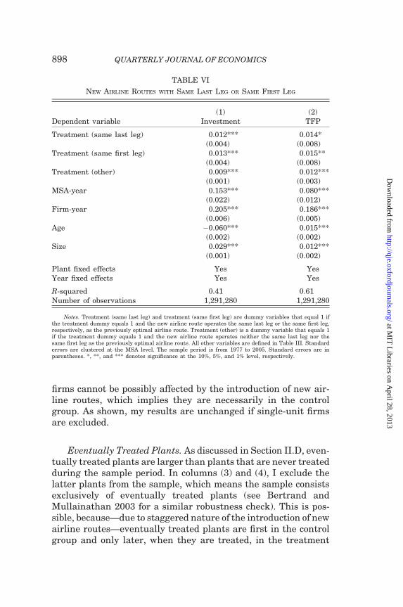
firms cannot be possibly affected by the introduction of new air-line routes, which implies they are necessarily in the controlgroup. As shown, my results are unchanged if single-unit firmsare excluded.

Eventually Treated Plants. As discussed in Section II.D, even-tually treated plants are larger than plants that are never treatedduring the sample period. In columns (3) and (4), I exclude thelatter plants from the sample, which means the sample consistsexclusively of eventually treated plants (see Bertrand andMullainathan 2003 for a similar robustness check). This is pos-sible, because—due to staggered nature of the introduction of newairline routes—eventually treated plants are first in the controlgroup and only later, when they are treated, in the treatment

TABLE VI

NEW AIRLINE ROUTES WITH SAME LAST LEG OR SAME FIRST LEG


Treatment (same last leg) 0.012*** 0.014*(0.004) (0.008)

Treatment (same first leg) 0.013*** 0.015**(0.004) (0.008)

Treatment (other) 0.009*** 0.012***(0.001) (0.003)

MSA-year 0.153*** 0.080***(0.022) (0.012)

Firm-year 0.205*** 0.186***(0.006) (0.005)

Age �0.060*** 0.015***(0.002) (0.002)

Size 0.029*** 0.012***(0.001) (0.002)



Notes. Treatment (same last leg) and treatment (same first leg) are dummy variables that equal 1 ifthe treatment dummy equals 1 and the new airline route operates the same last leg or the same first leg,respectively, as the previously optimal airline route. Treatment (other) is a dummy variable that equals 1if the treatment dummy equals 1 and the new airline route operates neither the same last leg nor thesame first leg as the previously optimal airline route. All other variables are defined in Table III. Standarderrors are clustered at the MSA level. The sample period is from 1977 to 2005. Standard errors are inparentheses. *, **, and *** denotes significance at the 10%, 5%, and 1% level, respectively.


at MIT

Libraries on A


Dow

nloaded from


TA

BL

EV

II

AL

TE

RN

AT

IVE

CO

NT

RO

LG

RO

UP

S

Mu

ltiu

nit

firm

sE

ven

tuall

ytr

eate

dp

lan

tsIn

crea

sein

travel

tim

e

(1)

(2)

(3)

(4)

(5)

(6)

Dep

end

ent

vari

able

Inves

tmen

tT

FP

Inves

tmen

tT

FP

Inves

tmen

tT

FP

Tre

atm

ent

0.0

09**

*0.0

12**

*0.0

11**

*0.0

10**

*0.0

09**

*0.0

13**

*(0

.001)

(0.0

03)

(0.0

02)

(0.0

03)

(0.0

01)

(0.0

03)

Incr

ease

intr

avel

tim

e�

0.0

05**

�0.0

08*

(0.0

02)

(0.0

05)

MS

A-y

ear

0.1

33**

*0.0

90**

*0.0

84**

0.0

84**

0.1

53**

*0.0

83**

*(0

.019)

(0.0

15)

(0.0

42)

(0.0

41)

(0.0

22)

(0.0

12)

Fir

m-y

ear

0.2

07**

*0.1

86**

*0.2

57**

*0.2

93**

*0.2

05**

*0.1

85**

*(0

.006)

(0.0

05)

(0.0

16)

(0.0

16)

(0.0

06)

(0.0

05)

Age

�0.0

72**

*0.0

13**

*�

0.0

47**

*0.0

38**

*�

0.0

60**

*0.0

15**

*(0

.002)

(0.0

03)

(0.0

04)

(0.0

09)

(0.0

02)

(0.0

02)

Siz

e0.0

26**

*0.0

20**

*0.0

27**

*0.0

25**

*0.0

29**

*0.0

12**

*(0

.001)

(0.0

02)

(0.0

02)

(0.0

06)

(0.0

01)

(0.0

02)

Pla

nt

fixed

effe

cts

Yes

Yes

Yes

Yes

Yes

Yes

Yea

rfi

xed

effe

cts

Yes

Yes

Yes

Yes

Yes

Yes

R-s

qu

are

d0.3

70.6

10.3

20.6

50.4

10.6

1N

um

ber

ofob

serv

ati

ons

825,0

97

825,0

97

70,4

67

70,4

67

1,2

82,2

28

1,2

82,2

28

Not

es.

Inco

lum

ns

(1)

an

d(2

),th

esa

mp

leis

rest

rict

edto

pla

nts

that

bel

ong

tom

ult

iun

itfi

rms

con

sist

ing

ofm

ore

than

one

esta

bli

shm

ent.

Inco

lum

ns

(3)

an

d(4

),th

esa

mp

leis

rest

rict

edto

pla

nts

that

are

even

tuall

ytr

eate

d—

that

is,

pla

nts

wh

ose

travel

tim

eto

hea

dqu

art

ers

isre

du

ced

thro

ugh

the

intr

odu

ctio

nof

an

ewair

lin

ero

ute

—d

uri

ng

the

sam

ple

per

iod

.In

crea

sein

travel

tim

eis

ad

um

my

vari

able

that

equ

als

1if

the

travel

tim

eto

hea

dqu

art

ers

incr

ease

sd

uri

ng

the

sam

ple

per

iod

du

eto

the

term

inati

onof

an

exis

tin

gair

lin

ero

ute

.A

llot

her

vari

able

sare

defi

ned

inT

able

III.

Sta

nd

ard

erro

rsare

clu

ster

edat

the

MS

Ale

vel

.T

he

sam

ple

per

iod

isfr

om1977

to2005.

Sta

nd

ard

erro

rsare

inp

are

nth

eses

.*,

**,

an

d**

*d

enot

essi

gn

ifica

nce

at

the

10%

,5%

,an

d1%

level

,re

spec

tivel

y.


at MIT

Libraries on A


Dow

nloaded from


group. As is shown, my results are similar if nontreated plantsare excluded.

Increases in Travel Time. In my main analysis, I consider onlythe introduction of new airline routes and not the termination ofexisting routes. Terminations are much less frequent than intro-ductions. Moreover, as routes that are discontinued are mostlyminor regional routes, the resulting increase in travel time (andthus the treatment effect) is likely to be modest. In columns(5) and (6), I add a second dummy that equals 1 whenever thetermination of an existing airline route leads to an increase intravel time between a plant and its headquarters. As shown, thecoefficient on this ‘‘increase in travel time’’ dummy is of the op-posite sign as the coefficient on the main treatment dummy,which is what one might expect. Importantly, however, the coef-ficient on the main treatment dummy remains unchanged (see,columns (2) and (5) of Table III), which implies my results areunaffected if I additionally account for the termination of existingairline routes.

IV.D. Miscellaneous Robustness Checks

Small versus Large Reductions in Travel Time. In the ana-lysis so far, any new airline route that reduces the travel timebetween a plant and its headquarters is coded as a treatment.Arguably, the treatment effect may be stronger for larger reduc-tions in travel time. To see whether this is true, I interact thetreatment dummy in equation (1) with a set of five dummiesindicating the magnitude of the travel time reduction: (�t � 30min), (�t > 30 min and �t � 1 hr), (�t > 1 hr and �t � 1 hr30 min), (�t > 1 hr 30 min and �t � 2 hr), and (�t > 2 hr),where �t is the reduction in travel time based on a one-waytrip. As Table A.3 in the Online Appendix shows, regardless ofwhether I use investment or TFP as the dependent variable, thetreatment effect is monotonic in the magnitude of the travel timereduction, is small and insignificant when the travel time reduc-tion is less than one hour (one way), and is strongest when thetravel time reduction exceeds two hours.

ASM Sample Weights. As described in Section II.A, the ASMincludes all manufacturing plants with more than 250 employees,


at MIT

Libraries on A


Dow

nloaded from




whereas smaller plants are randomly sampled every five years.As a result, the average plant in the sample is larger than theaverage U.S. manufacturing plant. Fortunately, the ASM con-tains plants’ sample weights—that is, the inverse of their sam-pling probabilities—which can be used to create a representativesample in terms of plant size (see, e.g., Greenstone, List, andSyverson 2011). Specifically, I reestimate my baseline regressionsby weighting observations either by their respective ASM sampleweight (for plant-weighting) or by the product of their respectiveASM sample weight and their deflated shipments (for dollar-weighting). The results are presented in Table A.4 in theOnline Appendix. Regardless of which weighting procedure Iuse, and regardless of whether I use investment or TFP as thedependent variable, the results are similar to those in Table III.

Alternative Measures of Productive Efficiency. My main meas-ure of plant-level productivity is TFP. A potential drawback of TFPis its reliance on structural assumptions (e.g., Cobb-Douglas pro-duction function). To assess the robustness of the TFP results, Iconsider two margin-based measures of plant-level productivitythat are free of such assumptions: return on capital (ROC) andoperating margin (OM). ROC is shipments minus labor and mater-ial costs, all divided by capital stock. OM is defined similarly, exceptthat the denominator is shipments. Both measures are industry-adjusted by subtracting the industry median in a given three-digitSIC industry and year. As is shown in columns (1) and (2) of TableA.5 in the Online Appendix, the results are similar to my baselineresults. This is not surprising, given that TFP is highly correlatedwith both ROC (60%) and OM (50%).

Another potential drawback is that in my main analysis, TFPis estimated by OLS. As discussed in Section II.C, this approach—though common in the literature (e.g., Schoar 2002; Bertrand andMullainathan 2003)—has been criticized on grounds that it givesrise to simultaneity and selection problems. In columns (3) and(4), I employ the structural techniques of Olley and Pakes (OP,1996) and Levinsohn and Petrin (LP, 2003), respectively, whichhave been designed to address these problems. As is shown, theresults are similar to my baseline results. This is again not sur-prising, given that the correlation between TFP estimated byOLS and TFP estimated using OP’s (LP’s) technique is 81%(84%).


at MIT

Libraries on A


Dow

nloaded from







V. Heterogeneity in the Treatment Effect

V.A. Headquarters’ Time Constraints

Monitoring requires that managers travel to plants. Thesame is true for collecting ‘‘soft’’ information, that is, informationthat ‘‘cannot be credibly transmitted’’ (Stein 2002, 1891) and‘‘cannot be directly verified by anyone other than the agent whoproduces it’’ (1892).33 Given that both activities are time-consuming, I would expect the treatment effect to be strongerfor plants whose headquarters is more time-constrained. Toexamine this hypothesis, I construct two measures of headquar-ters’ time constraints. The first measure is the number of man-agers employed at headquarters divided by the number of plantsof the firm (Managers/Plants). The second measure is the numberof managers employed at headquarters divided by the total dis-tance (in miles) between headquarters and all of the firm’s plants(Managers/Total Distance). The lower the ratio of managers toplants—or the greater the average distance the managers musttravel—the more time-constrained the headquarters.

A caveat is in order. When constructing these measures, I(somewhat generously) treated all of headquarters’ employeesas ‘‘managers.’’ Although it is true that all of headquarters’ em-ployees are white-collar employees, not all of them are managers.They may also include secretaries and clerical employees.Unfortunately, the Census data do not allow me to distinguishbetween managers and other white-collar employees. Neverthe-less, as long as the number of other white-collar employees isroughly proportional to the number of managers—which seemslike a reasonable assumption—this measurement error is un-likely to affect my results, for it merely implies that the numberof managers is scaled by a constant. Bearing this caveat in mind, Isort treated plants into two categories—‘‘high time constraints’’and ‘‘low time constraints’’—based on whether the measure oftime constraints is above or below the median of all treatedplants in the year prior to the treatment. Using pretreatmentvalues to sort plants mitigates concerns that the categorizationis affected by the treatment itself.

33. To provide further evidence that proximity to plants makes it easier forheadquarters to monitor and collect (soft) information about plants, I show inTable A.6 in the Online Appendix that the treatment effect is stronger for largerfirms and conglomerates, where one could plausibly argue that the loss of soft in-formation inside the firm hierarchy is larger.


at MIT

Libraries on A


Dow

nloaded from




An important limitation of my analysis is that the two meas-ures of headquarters’ time constraints—although computed inthe year prior to the treatment—are endogenous, for example,with respect to plant location or employment. Accordingly, theevidence presented next may not warrant a causalinterpretation.34

To examine whether the treatment effect is stronger forplants whose headquarters is more time-constrained, I interactthe treatment dummy in equation (1) with two dummies indicat-ing whether time constraints are low and high, respectively. Theresults are presented in Table VIII. In columns (1) and (3), thedependent variable is plant-level investment. As shown, thetreatment effect is between two and two and a half times strongerwhen time constraints are high. Specifically, in column (1), wheretime constraints are measured by ‘‘Managers/Plants,’’ the coeffi-cient on the interacted treatment dummy is 0.012 when time con-straints are high but only 0.006 when time constraints are low.The difference is significant at the 5% level (p=.028). The differ-ence becomes even more pronounced when the measure of head-quarters’ time constraints takes into account the geographicdispersion of plants. In column (3), where time constraints aremeasured by ‘‘Managers/Total Distance,’’ the coefficient on theinteracted treatment dummy is 0.013 when time constraintsare high but only 0.005 when time constraints are low. The dif-ference is now significant at the 1% level (p=.002). The resultswhen TFP is the dependent variable (columns (2) and (4)) mirrorthose for investment.

V.B. Innovations in Information Technology

The sample period from 1977 to 2005 witnessed major innov-ations in information technology. These innovations (e.g.,Internet, corporate intranet, video conferencing) facilitated infor-mation flows both within and across company units, reducing theneed to personally travel to plants. Accordingly, I would expectthe treatment effect to be stronger in the earlier years of my sam-ple period, where other, nonpersonal means of exchanging

34. In the absence of a concrete theory of optimal headquarters size and plantlocation, it is difficult to speculate what the direction or magnitude of a potentialbias might be.


at MIT

Libraries on A


Dow

nloaded from


information were either unavailable or less developed. To exam-ine this hypothesis, I interact the treatment dummy in equation(1) with three dummies indicating different time periods: before1986 (9 years), between 1986 and 1995 (10 years), and after 1995(10 years). The results are presented in Table IX. As is shown, thetreatment effect is indeed stronger in the earlier years of thesample period. When the dependent variable is plant investment,the coefficient on the interacted treatment dummy is 0.013 in thepre-1986 period, 0.010 in the period between 1986 and 1995, and0.005 in the post-1995 period. The difference between thepre-1986 and post-1995 coefficients is significant at the 5% level(p=.012). The results are similar when TFP is the dependentvariable.

TABLE VIII

HEADQUARTERS’ TIME CONSTRAINTS

Managers/plants Managers/total distance

(1) (2) (3) (4)Dependent variable Investment TFP Investment TFP

Treatment�hightime constraints

0.012*** 0.015*** 0.013*** 0.015***(0.002) (0.004) (0.002) (0.003)

Treatment� lowtime constraints

0.006*** 0.010** 0.005** 0.009*(0.002) (0.004) (0.002) (0.005)

MSA-year 0.153*** 0.080*** 0.153*** 0.080***(0.022) (0.012) (0.022) (0.012)

Firm-year 0.205*** 0.186*** 0.205*** 0.186***(0.006) (0.005) (0.006) (0.005)

Age �0.060*** 0.015*** �0.060*** 0.015***(0.002) (0.002) (0.002) (0.002)

Size 0.029*** 0.012*** 0.029*** 0.012***(0.001) (0.002) (0.001) (0.002)

Plant fixed effects Yes Yes Yes YesYear fixed effects Yes Yes Yes Yes

R-squared 0.41 0.61 0.41 0.61Number of observations 1,291,280 1,291,280 1,291,280 1,291,280

Notes. In columns (1) and (2), headquarters’ time constraints are measured as the number of(white-collar) employees at headquarters divided by the total number of plants of the company (‘‘man-agers/plants’’). In columns (3) and (4), headquarters’ time constraints are measured as the number of(white-collar) employees at headquarters divided by the total distance (in miles) between headquartersand all of the company’s plants (‘‘managers/total distance’’). High time constraints is a dummy variablethat equals 1 if the measure of headquarters’ time constraint lies above the median value across alltreated plants in the year prior to the treatment. Low time constraints is defined analogously. All othervariables are defined in Table III. Standard errors are clustered at the MSA level. The sample period isfrom 1977 to 2005. Standard errors are in parentheses. *, **, and *** denotes significance at the 10%, 5%,and 1% level, respectively.


at MIT

Libraries on A


Dow

nloaded from


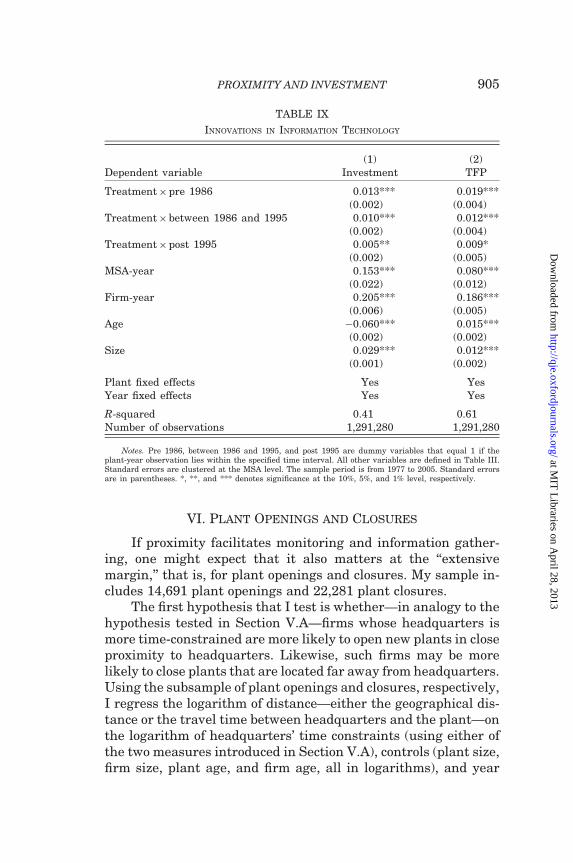
VI. Plant Openings and Closures

If proximity facilitates monitoring and information gather-ing, one might expect that it also matters at the ‘‘extensivemargin,’’ that is, for plant openings and closures. My sample in-cludes 14,691 plant openings and 22,281 plant closures.

The first hypothesis that I test is whether—in analogy to thehypothesis tested in Section V.A—firms whose headquarters ismore time-constrained are more likely to open new plants in closeproximity to headquarters. Likewise, such firms may be morelikely to close plants that are located far away from headquarters.Using the subsample of plant openings and closures, respectively,I regress the logarithm of distance—either the geographical dis-tance or the travel time between headquarters and the plant—onthe logarithm of headquarters’ time constraints (using either ofthe two measures introduced in Section V.A), controls (plant size,firm size, plant age, and firm age, all in logarithms), and year

TABLE IX

INNOVATIONS IN INFORMATION TECHNOLOGY


Treatment�pre 1986 0.013*** 0.019***(0.002) (0.004)

Treatment�between 1986 and 1995 0.010*** 0.012***(0.002) (0.004)

Treatment�post 1995 0.005** 0.009*(0.002) (0.005)

MSA-year 0.153*** 0.080***(0.022) (0.012)

Firm-year 0.205*** 0.186***(0.006) (0.005)

Age �0.060*** 0.015***(0.002) (0.002)

Size 0.029*** 0.012***(0.001) (0.002)



Notes. Pre 1986, between 1986 and 1995, and post 1995 are dummy variables that equal 1 if theplant-year observation lies within the specified time interval. All other variables are defined in Table III.Standard errors are clustered at the MSA level. The sample period is from 1977 to 2005. Standard errorsare in parentheses. *, **, and *** denotes significance at the 10%, 5%, and 1% level, respectively.


at MIT

Libraries on A


Dow

nloaded from


fixed effects.35 To mitigate concerns that plant openings or clos-ures might affect headquarters’ time constraints, I lag both meas-ures of time constraints by one year.

Importantly, although both measures of time constraints arelagged, the same caveat that applied in Section V.A also applieshere: The measures are endogenous. Specifically, the concern isthat there may be a persistent component in headquarters’ timeconstraints that correlates with omitted variables that in turnaffect the locations of plant openings or closures. Hence, the evi-dence presented below may not warrant a causal interpretation.

Table X contains the results. As is shown in columns (1) to(4), companies with more time-constrained headquarters areindeed more likely to open new plants in close proximity to head-quarters. Specifically, a one standard deviation reduction inheadquarters’ time constraints—that is, an increase in the meas-ures ‘‘Managers/Plants’’ or ‘‘Managers/Total Distance’’—is asso-ciated with a significant increase in distance of 29% to 39%.Likewise, as is shown in columns (5) to (8), companies withmore time-constrained headquarters are more likely to closeplants that are located far away from headquarters.

The second hypothesis that I test is whether—in analogy tothe hypothesis tested in Section V.B—over time, as innovations ininformation technology have reduced the need to travel to plants,the distance between headquarters and plants has increased.Specifically, I test whether firms have become more likely toopen new plants in distant locations and to close existing plantsin proximate locations. Using again the subsample of plant open-ings and closures, respectively, I regress the logarithm of dis-tance—either the geographical distance or the travel timebetween headquarters and the plant—on dummies indicatingthe time periods 1986 to 1995 and post-1995, respectively, andcontrols (plant size, firm size, plant age, and firm age, all in loga-rithms). The pre-1986 period constitutes the base group.

The results are presented in Table XI. As is shown in columns(1) and (2), the distance between headquarters and newly openedplants has increased by 18.5%–19% (29.7%–30.5%) from thepre-1986 period to the 1986–1995 (post–1995) period. The resultsfor plant closures in columns (3) and (4) mirror those for plant

35. Naturally, plant age is only included as a control in the plant closureregressions.


at MIT

Libraries on A


Dow

nloaded from


TA

BL

EX

HE

AD

QU

AR

TE

RS’

TIM

EC

ON

ST

RA

INT

SA

ND

PL

AN

TL

OC

AT

ION

Sam

ple

Pla

nt

open

ings

Pla

nt

clos

ure

s

Dep

end

ent

vari

able

Geo

gra

ph

ical

dis

tan

ceT

ravel

tim

eG

eogra

ph

ical

dis

tan

ceT

ravel

tim

e

(1)

(2)

(3)

(4)

(5)

(6)

(7)

(8)

Man

ager

s/p

lan

ts0.1

48**

*0.1

21**

*�

0.2

09**

*�

0.1

92**

*(0

.027)

(0.0

22)

(0.0

19)

(0.0

15)

Man

ager

s/to

tal

dis

tan

ce0.4

24**

*0.3

13**

*�

0.4

28**

*�

0.3

50**

*(0

.010)

(0.0

09)

(0.0

09)

(0.0

08)

Fir

msi

ze0.5

57**

*0.3

14**

*0.4

39**

*0.2

59**

*0.6

47**

*0.3

62**

*0.5

43**

*0.3

14**

*(0

.014)

(0.0

14)

(0.0

11)

(0.0

11)

(0.0

14)

(0.0

15)

(0.0

10)

(0.0

10)

Fir

mage

0.5

23**

*0.3

84**

*0.5

44**

*0.4

42**

*0.7

28**

*0.4

96**

*0.7

01**

*0.5

10**

*(0

.041)

(0.0

36)

(0.0

37)

(0.0

33)

(0.1

00)

(0.0

89)

(0.0

89)

(0.0

78)

Siz

e�

0.2

79**

*�

0.1

73**

*�

0.2

46**

*�

0.1

69**

*�

0.2

82**

*�

0.1

79**

*�

0.2

51**

*�

0.1

70**

*(0

.018)

(0.0

16)

(0.0

14)

(0.0

13)

(0.0

13)

(0.0

12)

(0.0

10)

(0.0

09)

Age

�0.3

04**

*�

0.2

57**

*�

0.2

84**

*�

0.2

46**

*(0

.034)

(0.0

31)

(0.0

25)

(0.0

23)

Yea

rfi

xed

effe

cts

Yes

Yes

Yes

Yes

Yes

Yes

Yes

Yes

R-s

qu

are

d0.2

70.3

90.2

80.3

80.3

80.4

80.4

00.4

9N

um

ber

ofob

serv

ati

ons

14,6

91

14,6

91

14,6

91

14,6

91

22,2

81

22,2

81

22,2

81

22,2

81

Not

es.

Th

esa

mp

leof

pla

nt

open

ings

(clo

sure

s)in

colu

mn

s(1

)–(4

)((

5)–

(8))

incl

ud

esall

sam

ple

pla

nts

that

are

cod

edas

‘‘bir

th’’

(‘‘d

eath

’’)in

the

LB

D.

Geo

gra

ph

ical

dis

tan

ceis

the

natu

ral

logari

thm

ofon

ep

lus

the

gre

at-

circ

led

ista

nce

bet

wee

nth

ep

lan

t’s

ZIP

cod

ean

dth

eZ

IPco

de

ofh

ead

qu

art

ers.

Tra

vel

tim

eis

the

natu

ral

logari

thm

ofon

ep

lus

the

tota

ltr

avel

tim

ebase

don

the

fast

est

rou

tean

dm

ean

sof

tran

spor

tati

on(c

ar

orp

lan

e)bet

wee

nth

ep

lan

t’s

ZIP

cod

ean

dth

eZ

IPco

de

ofh

ead

qu

art

ers.

Fir

msi

zeis

the

natu

ral

logari

thm

ofth

eto

tal

nu

mber

ofem

plo

yee

sof

the

pare

nt

com

pan

yto

wh

ich

the

pla

nt

bel

ongs.

Fir

mage

isth

en

atu

ral

logari

thm

ofon

ep

lus

the

nu

mber

ofyea

rsth

ep

are

nt

com

pan

yh

as

bee

nin

the

LB

D.

All

oth

ervari

able

sare

defi

ned

inT

able

III.

Sta

nd

ard

erro

rsare

clu

ster

edat

the

MS

Ale

vel

.T

he

sam

ple

per

iod

isfr

om1977

to2005.

Sta

nd

ard

erro

rsare

inp

are

nth

eses

.*,

**,

an

d**

*d

enot

essi

gn

ifica

nce

at

the

10%

,5%

,an

d1%

level

,re

spec

tivel

y.


at MIT

Libraries on A


Dow

nloaded from


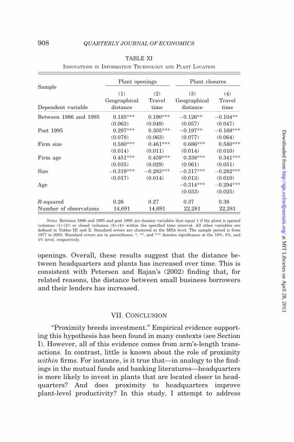
openings. Overall, these results suggest that the distance be-tween headquarters and plants has increased over time. This isconsistent with Petersen and Rajan’s (2002) finding that, forrelated reasons, the distance between small business borrowersand their lenders has increased.

VII. Conclusion

‘‘Proximity breeds investment.’’ Empirical evidence support-ing this hypothesis has been found in many contexts (see SectionI). However, all of this evidence comes from arm’s-length trans-actions. In contrast, little is known about the role of proximitywithin firms. For instance, is it true that—in analogy to the find-ings in the mutual funds and banking literatures—headquartersis more likely to invest in plants that are located closer to head-quarters? And does proximity to headquarters improveplant-level productivity? In this study, I attempt to address

TABLE XI

INNOVATIONS IN INFORMATION TECHNOLOGY AND PLANT LOCATION

SamplePlant openings Plant closures

(1) (2) (3) (4)

Dependent variableGeographical Travel

timeGeographical Travel

timedistance distance

Between 1986 and 1995 0.185*** 0.190*** �0.126** �0.104**(0.063) (0.049) (0.057) (0.047)

Post 1995 0.297*** 0.305*** �0.197** �0.168***(0.078) (0.063) (0.077) (0.064)

Firm size 0.580*** 0.461*** 0.686*** 0.580***(0.014) (0.011) (0.014) (0.010)

Firm age 0.451*** 0.459*** 0.338*** 0.341***(0.035) (0.029) (0.061) (0.051)

Size �0.319*** �0.283*** �0.317*** �0.282***(0.017) (0.014) (0.013) (0.010)

Age �0.314*** �0.294***(0.033) (0.025)

R-squared 0.26 0.27 0.37 0.39Number of observations 14,691 14,691 22,281 22,281

Notes. Between 1986 and 1995 and post 1995 are dummy variables that equal 1 if the plant is opened(columns (1)–(2)) or closed (columns (3)–(4)) within the specified time interval. All other variables aredefined in Tables III and X. Standard errors are clustered at the MSA level. The sample period is from1977 to 2005. Standard errors are in parentheses. *, **, and *** denotes significance at the 10%, 5%, and1% level, respectively.


at MIT

Libraries on A


Dow

nloaded from


these questions using plant-level data from the U.S. CensusBureau. My contribution is to provide plausibly exogenous vari-ation in the proximity between headquarters and plants.Specifically, I notice that the main reason empirical studies areinterested in (geographical) proximity is because it proxies for theease of monitoring and acquiring information. I argue that a moredirect proxy is travel time. Using the introduction of new airlineroutes as a source of exogenous variation in plants’ proximity toheadquarters, I estimate the effects on plant-level investmentand productivity. I find that new airline routes that reduce thetravel time between headquarters and plants lead to an increasein plant-level investment of 8% to 9% and to an increase in plants’total factor productivity of 1.3% to 1.4%, corresponding to an in-crease in plant-level profits of $275,000 to $296,000 (in 1997dollars).

Although these magnitudes represent the average treatmenteffect, there is substantial heterogeneity. For instance, thetreatment effect is stronger for plants whose headquarters ismore time-constrained, consistent with the notion that time con-straints limit the ability of headquarters to monitor and acquireinformation about plants. Also, I show that the results are stron-ger in the earlier years of the sample period, where other, non-personal means of exchanging information (e.g., Internet,corporate intranet, video conferencing) were either unavailableor less developed. Finally, I provide auxiliary evidence suggest-ing that monitoring and information acquisition are potentiallyimportant determinants of plant location. Specifically, I showthat companies whose headquarters is more time-constrained aremore likely to open plants in close proximity to headquarters andclose plants that are located far away from headquarters.Similarly, over time—as innovations in information technologyhave reduced the need to travel to plants—firms have becomemore likely to open new plants in distant locations and closeexisting plants in proximate locations, implying the distancebetween headquarters and plants has increased.

Appendix A: Location of Headquarters

The primary source of headquarters data is the AES, whichcontains information on auxiliary establishments every five yearsfrom 1977 to 2002. An auxiliary is any establishment whose


at MIT

Libraries on A


Dow

nloaded from


principal function is to ‘‘manage, administer, service, or supportthe activities of the company’s other establishments’’ (U.S.Census Bureau 1996, 133). Auxiliary establishments includeheadquarters, warehouses, garages, and other facilities primarilyengaged in servicing a company’s operating establishments.

To distinguish between headquarters and other auxiliaryestablishments, I use the selection criteria employed in Aarlandet al. (2007). Specifically, in 1997 and 2002, headquarters is iden-tified by the six-digit NAICS industry code 551114.36 In prioryears (1977, 1982, 1987, and 1992)—that is, before the introduc-tion of NAICS codes by the Census Bureau—headquarters isidentified as an establishment for which the joint category ofmanagement, administrative, and clerical employees dominateseach of the other employment categories.

These criteria do not differentiate between a company’s mainheadquarters and regional or divisional administrative offices. Asa result, they may yield more than one ‘‘headquarters’’ per com-pany. In my manufacturing sample, 20% of the multiunit compa-nies have multiple headquarters in the AES. To identify the mainheadquarters, I supplement the AES with information from theSSEL. The SSEL contains the names and addresses of all U.S.business establishments. This information typically includes abrief description of the establishment. Accordingly, I search forkeywords that explicitly point to the main headquarters (such as‘‘corporate headquarters’’ or ‘‘company headquarters’’). This pro-cedure identifies the main headquarters for 24% of the companieswith multiple headquarters. For the remaining companies, I sup-plement the AES with payroll information from the LBD. Themain headquarters is then identified as the headquarters withthe highest payroll. The intuition behind this criterion is twofold.First, the main company headquarters is likely to be substan-tially larger than either regional or divisional administrativeoffices. Second, the main headquarters employs the CEO andmost senior executives of the company, whose salaries arelikely to translate into relatively higher payroll figures.

36. The NAICS Industry 551114 comprises ‘‘establishments (except govern-ment establishments) primarily engaged in administering, overseeing, and mana-ging other establishments of the company or enterprise. These establishmentsnormally undertake the strategic or organizational planning and decision-making role of the company or enterprise. Establishments in this industry mayhold the securities of the company or enterprise’’ (U.S. Census Bureau 2000,Appendix B).


at MIT

Libraries on A


Dow

nloaded from


Not all multiunit companies have headquarters data in theAES. Because by definition, auxiliary establishments are physi-cally separated from production facilities, the AES covers onlystand-alone headquarters. For example, headquarters that areintegrated into manufacturing plants are classified as manufac-turing establishments and appear in the CMF. To determine theheadquarters’ location of companies without stand-alone head-quarters, I apply similar criteria as above. Specifically, all LBDestablishments of the company are matched to the SSEL.Whenever the name and address provided in the SSEL is notsufficient to determine the corporate headquarters, I select theestablishment with the highest payroll from the LBD (or thehighest white-collar payroll from the CMF if all establishmentsare manufacturing plants). Arguably, the latter criterion is sub-ject to misclassification if, for example, headquarters is located inthe smallest plant of the company. Fortunately, the impact ofsuch misclassification is likely to be small. In my sample of man-ufacturing firms, companies without stand-alone headquartersare mainly small companies with only a few plants. Theseplants are typically located in the same MSA or county, whichmakes air travel an unlikely means of transportation betweenheadquarters and the plants. My results are unaffected if Iexclude these plants from the sample.

To assess the accuracy of the headquarters location obtainedfrom the Census micro data, I merge my data set with Compustatusing the Compustat-SSEL bridge maintained by the CensusBureau. Compustat contains firm-level information on large pub-licly traded U.S. companies, including the ZIP code of the com-pany’s headquarters. A drawback is that Compustat’s ZIP codesare available only for the latest available year of the database andmay therefore be an incorrect benchmark for companies whoseheadquarters has moved since the last AES year. Nevertheless,this inaccuracy will merely understate the actual match betweenheadquarters locations from Compustat and the Census microdata. The merged sample consists of 4,045 companies correspond-ing to 312,774 plant-year observations. The headquarters loca-tion is the same for 84% of the companies, which account for91% of the plant-year observations. Though this match may beconsidered satisfactory, I have verified that my results are simi-lar if I restrict the sample to the publicly traded companies listedin Compustat and use the headquarters ZIP codes fromCompustat instead.


at MIT

Libraries on A


Dow

nloaded from


Appendix B: Variables of the Production Function

This appendix describes how the variables of the productionfunction are constructed. Unless otherwise specified, all variablesare measured at the plant level and are obtained from the long-itudinal linkage of the CMF and ASM.

Output is the total value of shipments plus changes in thevalue of inventories for finished goods and work in process,divided by the four-digit SIC shipment deflator from the NBER-CES Manufacturing Industry Database. Material is the sum ofcost of materials and parts, cost of fuels, cost of purchased elec-tricity, cost of resales, and cost of contract work, divided by thefour-digit SIC material deflator from the NBER-CES Manufac-turing Industry Database. Labor is measured in ‘‘productionworker-equivalent hours’’ using the procedure described in Lich-tenberg (1992). Specifically, labor is calculated as productionworker hours times the ratio of total wages (including supplemen-tal labor costs) to wages of production workers. This procedureassumes that the ratio of production to nonproduction wage ratesis equal to the ratio of their marginal products.

Following Lichtenberg (1992), capital is calculated using theperpetual inventory method. This method requires an initialvalue of real capital stock. For each plant, I select the earliestavailable book value of capital. To account for depreciation, Imultiply this value by the two-digit SIC adjustment factor fromthe Bureau of Economic Analysis (BEA). This adjustment factoris the ratio of industry net capital stock in current dollars toindustry gross capital stock in historical dollars. The adjustedbook value of capital is then divided by the four-digit SIC invest-ment deflator from the NBER-CES Manufacturing IndustryDatabase. If the earliest available book value of capital corre-sponds to the year in which the plant was ‘‘born’’ (as identifiedby the ‘‘birth’’ flag in the LBD), no adjustment for depreciation isneeded. In this case, the book value is simply divided by the four-digit SIC investment deflator.

The initial value of real capital stock is then written forwardusing the recursive perpetual inventory formula

Kit ¼ Kit�1 � ð1� �itÞ þ Iit,

where i indexes plants, t indexes years, K is the value of realcapital stock, d is the two-digit SIC depreciation rate from theBEA, and I is capital expenditures divided by the four-digit SIC


at MIT

Libraries on A


Dow

nloaded from


investment deflator. Until the 1997 Census, all necessary vari-ables are available separately for buildings and machinery.Accordingly, I calculate the capital stock for each asset categoryand add them together to obtain the final measure of capitalstock. As of 1997, only aggregate capital stock variables are avail-able. Another limitation is that in 1986 as well as after the 1987Census, no questions are asked about assets in the ASM.However, questions about capital expenditures are asked everyyear. Accordingly, for plants that enter in 1986 or betweenCensus years after 1987, I use asset information from the CMFin the following Census year and iterate the recursive perpetualinventory formula backward to construct capital stock in the pre-ceding ASM years (e.g., if a plant enters in 1989, I use assetinformation from the 1992 CMF and iterate the formula back-ward to obtain capital stock for 1989–1991). Plants whose birthand death occur between two Census years post 1987 are droppedfrom the sample because capital stock cannot be constructed. Fora more detailed discussion of these issues, see the data appendixin Abraham and White (2006).

Massachusetts Institute of Technology

SUPPLEMENTARY MATERIAL

An Online Appendix for this article can be found at QJEonline (qje.oxfordjournals.org).

References

Aarland, Kristin, James C. Davis, J. Vernon Henderson, and Yukako Ono,‘‘Spatial Organization of Firms: The Decision to Split Production andAdministration,’’ RAND Journal of Economics, 38 (2007), 480–494.

Abraham, Arpad, and Kirk White, ‘‘The Dynamics of Plant-Level Productivity inU.S. Manufacturing,’’ CES Working Paper 06-20, 2006.

Ackerberg, Daniel A., C. Lanier Benkard, Steven Berry, and Ariel Pakes,‘‘Econometric Tools for Analyzing Market Outcomes,’’ in Handbook ofEconometrics, James J. Heckman, and Edward E. Leamer, eds.(Amsterdam: Elsevier/North-Holland, 2007).

Aghion, Philippe, and Jean Tirole, ‘‘Formal and Real Authority in Organizations,’’Journal of Political Economy, 105 (1997), 1–29.

Bertrand, Marianne, and Sendhil Mullainathan, ‘‘Enjoying the Quiet Life?Corporate Governance and Managerial Preferences,’’ Journal of PoliticalEconomy, 111 (2003), 1043–1075.

Bertrand, Marianne, Esther Duflo, and Sendhil Mullainathan, ‘‘How MuchShould We Trust Differences-in-Differences Estimates?’’ Quarterly Journalof Economics, 119 (2004), 249–275.

Bordalo, Pedro, Nicola Gennaioli, and Andrei Shleifer, ‘‘Salience Theory of Choiceunder Risk,’’ Quarterly Journal of Economics, 127 (2012), 1243–1285.


at MIT

Libraries on A


Dow

nloaded from



Core, John, and Wayne Guay, ‘‘Estimating the Value of Employee Stock OptionPortfolios and their Sensitivities to Price and Volatility,’’ Journal ofAccounting Research, 40 (2002), 613–630.

Coval, Joshua D., and Tobias J. Moskowitz, ‘‘Home Bias at Home: Local EquityPreference in Domestic Portfolios,’’ Journal of Finance, 54 (1999), 2045–2074.

———, ‘‘The Geography of Investment: Informed Trading and Asset Prices,’’Journal of Political Economy, 109 (2001), 811–841.

Cremer, Jacques, ‘‘Arm’s Length Relationships,’’ Quarterly Journal of Economics,110 (1995), 275–295.

DellaVigna, Stefano, ‘‘Psychology and Economics: Evidence from the Field,’’Journal of Economic Literature, 47 (2009), 315–372.

Edgerton, Jesse, ‘‘Agency Problems in Public Firms: Evidence from Corporate Jetsin Leveraged Buyouts,’’ Journal of Finance, 67 (2012), 2187–2214.

Foster, Lucia, John C. Haltiwanger, and Chad Syverson, ‘‘Reallocation FirmTurnover, and Efficiency: Selection on Productivity or Profitability?’’American Economic Review, 98 (2008), 394–425.

Gabaix, Xavier, David Laibson, Guillermo Moloche, and Stephen Weinberg,‘‘Costly Information Acquisition: Experimental Analysis of a BoundedlyRational Model,’’ American Economic Review, 96 (2006), 1043–1068.

Gennaioli, Nicola, and Andrei Shleifer, ‘‘What Comes to Mind,’’ Quarterly Journalof Economics, 125 (2010), 1399–1433.

Giroud, Xavier, and Holger M. Mueller, ‘‘Capital and Labor Reallocation InsideFirms,’’ Mimeo, Massachusetts Institute of Technology, 2012.

Goetz, Andrew R., and Christopher J. Sutton, ‘‘The Geography of Deregulation inthe U.S. Airline Industry,’’ Annals of the Association of AmericanGeographers, 87 (1997), 238–263.

Greenstone, Michael, John A. List, and Chad Syverson, ‘‘The Effects ofEnvironmental Regulation on the Competitiveness of U.S. Manufacturing,’’CES Working Paper 11-03, 2011.

Harris, Milton, and Artur Raviv, ‘‘The Capital Budgeting Process: Incentives andInformation,’’ Journal of Finance, 51 (1996), 1139–1174.

Ivy, Russell L., ‘‘Variations in Hub Service in the US Domestic Air TransportationNetwork,’’ Journal of Transport Geography, 1 (1993), 211–218.

Jarmin, Ron S., and Javier Miranda, ‘‘The Longitudinal Business Database,’’ CESWorking Paper 02-17, 2003.

Kroc, Ray. Grinding it Out: The Making of McDonald’s (New York: St. Martin’sPaperbacks, 1992).

Lerner, Josh, ‘‘Venture Capitalists and the Oversight of Private Firms,’’ Journalof Finance, 50 (1995), 301–318.

Levinsohn, James, and Amil Petrin, ‘‘Estimating Production Functions UsingInputs to Control for Unobservables,’’ Review of Economic Studies, 70(2003), 317–341.

Lichtenberg, Frank R. Corporate Takeovers and Productivity (Cambridge, MA:MIT Press, 1992).

Malenko, Andrey, ‘‘Optimal Design of Internal Capital Markets,’’ Mimeo,Stanford University, 2011.

Mian, Atif, ‘‘Distance Constraints: The Limits of Foreign Lending in PoorEconomies,’’ Journal of Finance, 61 (2006), 1465–1505.

Michaels, Guy, ‘‘The Effect of Trade on the Demand for Skill — Evidence from theInterstate Highway System,’’ Review of Economics and Statistics, 90 (2008),683–701.

National Business Aviation Administration, NBAA Business Aviation FactBook 2004 (Washington, DC: National Business Aviation Administration,2004).

Olley, Steven G., and Ariel Pakes, ‘‘The Dynamics of Productivity in theTelecommunications Equipment Industry,’’ Econometrica, 64 (1996),1263–1297.

Petersen, Mitchell A., and Raghuram G. Rajan, ‘‘Does Distance Still Matter? TheInformation Revolution in Small Business Lending,’’ Journal of Finance, 57(2002), 2533–2570.

Schoar, Antoinette, ‘‘The Effect of Diversification on Firm Productivity,’’ Journalof Finance, 62 (2002), 2379–2403.


at MIT

Libraries on A


Dow

nloaded from


Seru, Amit, ‘‘Firm Boundaries Matter: Evidence from Conglomerates and R&DActivity,’’ Journal of Financial Economics (forthcoming).

Stein, Jeremy C., ‘‘Internal Capital Markets and the Competition for CorporateResources,’’ Journal of Finance, 52 (1997), 111–133.

———, ‘‘Information Production and Capital Allocation: Decentralized vs.Hierarchical Firms,’’ Journal of Finance, 57 (2002), 1891–1921.

Sufi, Amir, ‘‘Information Asymmetry and Financing Arrangements: Evidencefrom Syndicated Loans,’’ Journal of Finance, 62 (2007), 629–668.

Syverson, Chad, ‘‘Market Structure and Productivity: A Concrete Example,’’Journal of Political Economy, 112 (2004), 1181–1222.

———, ‘‘What Determines Productivity?’’ Journal of Economic Literature, 49(2011), 326–365.

Tirole, Jean, The Theory of Corporate Finance (Princeton, NJ: PrincetonUniversity Press, 2006).

U.S. Census Bureau, History of the 1992 Economic Census (Washington, DC: U.S.Government Printing Office, 1996).

———, 1997 Economic Census: Management of Companies and Enterprises(Washington, DC: U.S. Government Printing Office, 2000).

Yermack, David, ‘‘Flights of Fancy: Corporate Jets, CEO Perquisites, and InferiorShareholder Returns,’’ Journal of Financial Economics, 80 (2006), 211–242.


at MIT

Libraries on A


Dow

nloaded from


i. introduction - columbia universityxg2285/proximity.pdf · thank my advisor, holger mueller; ......

Documents