I

Ordered Sets via Adjunctions

R.J. Wood

‘Sets for Mathematics’, by F.W. Lawvere and R. Rosebrugh, [5] is a ground-breaking, undergraduate, set theory textbook. Categories provide the metalan-guage and, for a substantial part of the book, axioms are gradually imposed ona category S until its objects and arrows capture the key features of sets andfunctions that are used in mathematical practice. To those who would say thatsets and functions are themselves lurking in the definition of category the rejoin-der should surely be that sets and functions are present to the same extent inthe metalanguage of traditional set theory texts. By the time a student starts tothink critically about sets and functions in an undergraduate mathematics pro-gramme, he or she has already implicitly studied several categories — continuous,differentiable, linear, order-preserving, and so on. It is to these categories, andother categories of mathematical structures, that a student turns repeatedly inthe course of studying Mathematics. To see these categories as categories of setswith structure, it seems to this writer most appropriate to put the formal studyof sets themselves on the same footing.

Lawvere and Rosebrugh accomplish in [5] much more than is possible in atraditional set theory book because they isolate those categorical axioms for setsand functions that allow sets to admit both variation and the intuitionisticallyvalid constructs and theorems of the subject. A category satisfying the axiomsin question is called a(n elementary) topos. For each topos S there is a categoryof groups in S, of topological spaces in S, and so on. Rather remarkably, suchcategories can be studied as though their objects are sets with structure, usingquite conventional methodology, provided that one proceeds as an intuitionist.Part of the goal of this chapter is to make a modest incursion into the ‘category’of ordered objects in a topos.

For undergraduate students, much of the material in [5] is a serious prerequisitefor this chapter. At the time of this writing, [5] itself is very new but most of thematerial it contains has been known to the category theory community for aboutthirty years and certainly there are category theorists who have taught set theoryclasses to their undergraduates employing the ideas of [5] but without benefit ofa published text. There are other texts on toposes which, strictly speaking, couldserve as prerequisites for this work but they are aimed at a higher level than this

6 I. Ordered Sets

chapter itself. For readers familiar with topos theory via older texts, it is hopedthat the present contribution may serve as reference material.

Just as there is a category of groups in S (S a topos) so there is a categorywhose objects are categories in S and whose arrows are functors. After all, inthe metalanguage of categories, wherein S itself appears, we speak of a categoryas having a ‘set’ of objects, a ‘set’ of arrows, and functions, satisfying functionalidentities, that prescribe domain, codomain, identity arrows and composition. Ifthe set theory given by S is to be taken at all seriously then it is quite natural tospeak of categories in S. (In fact, less than the full set of axioms for a topos sufficesfor this purpose.) Let us write cat(S) for the category of categories and functorsin S. For F,G : X -A in cat(S) it is a straightforward matter to define naturaltransformations from F to G — just as in the metalanguage — and, with these athand, to define adjunction in cat(S) — again, just as in the metalanguage.

To some, including this writer, adjunction is the most important concept incategory theory. Its foundational nature is witnessed by the fact that the axioms fora topos can be given in terms of adjunctions. Yet, adjunction tends to appear ratherlate in most accounts of category theory and is often presented in a forbiddinglytechnical way. Fortunately, the concept makes sense for order-preserving functionsand for these it is almost impossible to obfuscate the central ideas.

A student who has studied but a little of [5] already knows that if a categoryC of the metalanguage has the property that, for any objects X and A in C, thereis at most one arrow from X to A then C is an ‘ordered set’ and that one might aswell write X ≤ A precisely when there is an arrow from X to A. Such a studentalso knows that if categories C and D are both ‘ordered sets’ in this sense then togive a functor F : C -D is to give a function from the objects of C to the objectsof D with the property that X ≤ A implies FX ≤ FA. We assume this familiarityin the process of defining ord(S), as the bicategory of ordered objects in S, order-preserving arrows, and inequalities. We then immediately define adjunction inord(S) and keep it as a central theme throughout.

We say no more about cat(S). By concentrating on adjunction in ord(S) weare able to pursue the concept without coming to terms with the issues of ‘size’and ‘coherence’ while at the same time somewhat advancing the programme of [5]in an obvious direction. One might make the case for simply pursuing the studyof ordered sets via adjunction in the metalanguage but to do so would lose sightof the valuable generality gained in [5]. Most of what we chose to include is validin any topos. We find it convenient to write set for S and ord for ord(S) and wedo not give any explicit examples of how our set might be variable because theseare to be found in [5]. The student who has carefully studied [5] is encouraged toexamine key concepts of this chapter in toposes such as set2 by translating themback to set.

Of course the study of ordered sets can be taken up in many ways using tra-ditional foundations and there are some serious limitations on what we can hopeto say without introducing more pure topos theory than is already found in [5].An important case in point concerns the issue of finiteness. In our set there are

Introduction 7

different, inequivalent notions of finiteness that must be employed for a carefultreatment of some theorems that are traditionally quite straightforward. We donot pursue this problem. On the few occasions when we find it convenient, for ex-pository reasons, to include material that addresses finiteness we flag such resultswith an asterisk.

In Section 1 we provide some preliminaries that allow us to build ordered settheory from the bicategory of relations in set. In fact we define adjunctions therein,and show that from these we can recover functions. In Section 2 we formallydefine ordered sets, the bicategory of these, adjunctions therein, and provide someimportant examples. We put adjunctions to work in Section 3 to describe semi-lattices, lattices and a few of their specializations. So as to discuss complete latticesin these terms in Section 5, Section 4 addresses power set Heyting algebras.

Of course power sets are traditionally considered to be Boolean algebras andhere we should underscore a central point of departure with traditional approaches.We do not assume of our set that a subset of a set is equal to its double ‘com-plement’ — in other words we do not assume that our topos set is Boolean. (Afortiori, we do not invoke the axiom of choice, which is known to imply Booleaness— a fact first discovered in the context of topos theory by Radu Diaconescu.)Actually, independently of any wish to work in a topos, there is a certain economywhen it comes to ordered sets in confronting Heyting rather than Boolean algebrafrom the outset. For an ordered set, in anybody’s set theory, the downsets of theordered set (ordered by inclusion) form a Heyting rather than a Boolean algebra.It is the downsets of an ordered set X (which we fully intend to pursue in somedetail) that are relevant to the study of X in a way that the power set of theunderlying set of X cannot be expected to be. After all, most sets can be orderedin more than one way, in anybody’s set theory. Ordered set theory in particular— category theory in general — is intrinsically intuitionistic.

Section 6 is a brief introduction to the author’s own work on completely dis-tributive lattices with a number of coauthors, most notably Rosebrugh. It is herethat the approach to ordered sets via adjunction seems to add the greatest clarityto the subject to date.

Traditionally, most theorems about completely distributive (CD) lattices haveinvoked the axiom of choice (AC). In fact, without (AC) there is even a paucity ofexamples of (CD) lattices, for one of the many classical equivalent forms of (AC)states that every power set is (CD). Via adjunction it is very natural to introduce anotion that we have called ‘constructively completely distributive’ (CCD) latticesfor which we prove the following theorem, stated in an obvious symbolic form:

(AC)⇐⇒ ((CD)⇐⇒ (CCD))

Via adjunction it follows, almost immediately from the definition of (CCD), thatevery power set is intuitionistically (CCD) (and together with the aforementionedclassical result about power sets this proves half of the assertion above).

In fact, (CCD) bears further on the issue of studying Mathematics via topostheory. Let us write (opCD) for the dual of (CD). In other words, a lattice L

8 I. Ordered Sets

satisfies (opCD) if and only if the dual lattice Lop satisfies (CD). Similarly, write(opCCD) for the dual of (CCD). It is classical that

(AC) =⇒ ((CD)⇐⇒ (opCD))

Writing (BLN) to denote that the topos of enquiry is Boolean, it was shown in [7]that

(BLN)⇐⇒ ((CCD)⇐⇒ (opCCD))

We include a proof of this result and observe that it, together with other resultsof this section, provides a new, indirect proof of the aforementioned Diaconescuresult:

(AC) =⇒ (BLN)

1. Preliminaries

1.1. Categorical prerequisites. We assume a basic knowledge of categorical con-cepts, such as pullback, which are defined by universal mapping properties. Anexcellent reference is [5]. The study of ordered sets allows one to meet new exam-ples — simultaneously on two different levels. We will see that on the one hand,ordered sets and the relevant functions between them form a category but, onthe other hand, each ordered set can be regarded as a category in its own right.Thus, the category of all ordered sets will provide a simple example of a categoryof categories.

1.2. Topos axioms. A topos, see [5], is a category S which has

i) finite limits;ii) power objects.

From the axioms it follows that a topos has finite colimits, mapping objects, a sub-object classifier, and many other properties. Often, ii) is expressed in the contextof i) by saying of S that it

ii′) is cartesian closed (has mapping objects);ii′′) has a subobject classifier.

If Ω is a subobject classifier for cartesian closed S with finite limits then, for each Xin S, a power object is provided by ΩX . Conversely, if S with finite limits has powerobjects PX then P1, where 1 is the terminal object, provides a subobject classifierwhile power objects AX are obtained as certain subobjects of the P(A×X).

As stated in the introduction, we will write set for the topos that is regardedas our category of sets and functions and, unless otherwise indicated, assume nomore than that. In particular, we do not assume that the PX are Boolean algebrasin set. In set we speak of ‘power sets’, and so on, rather than ‘power objects’.

1. Preliminaries 9

1.3. Specified universal objects. We will understand ‘has’ in connection withfinite limits and power sets to include specification. For if in some category wehave squares

A X-f

P B-q

?

p

?

g

A X-f

P ′ B-q′

?

p′

?

g

which are pullbacks then there is an isomorphism i : P '- P ′, unique with theproperty that

p′@@I

P

A

p

P ′?

iq′

B

q@@R

commutes. Either square is ‘a’ pullback of f and g and without further comment‘the’ pullback of f and g might be meaningless without making some sort ofchoice. In many categories however there is a specific construction which producesa specific pullback, for each pair f and g with common codomain. It is our pointof view that set is such a category but we have no need to say what the specificconstruction is. When we speak of ‘the’ pullback of f and g this specific pullback iswhat we will mean. Notation such as A×X B will be used for specified pullbacks.In particular, set has specified inverse images of parts (monomorphisms) too andnotation such as f−1(m) will be used for these. We make similar conventions aboutthe terminal set and the power set of a given set. It follows that we have derivedspecifications — for colimits and so on. It should be noted though that specifiedpullbacks and the like do not enjoy many closure properties. For example, if twopullback squares are pasted side by side then the resulting large square is againa pullback but it is usually not a specified pullback when the original pullbacksquares are so.

1.4. Categories of parts. For X any set, we provisionally write PX for the collec-tion of all parts of X. (A part of X is a monomorphism with codomain X.) Hereand in the sequel the word ‘collection’ will be used as a term in the metalanguagethat we are tacitly using to describe our category set of sets and functions. Ifgiven collections Q and R there is a rule φ that associates to each Q in Q a uniqueR in R then we use notation such as φ(Q) = R and even φ : Q -R, withoutthe suggestion that φ : Q -R is in set or for that matter in any other categoryunder formal consideration. Such notation is merely a convenient extension of themetalanguage. In fact, such Q and R can be seen as discrete categories, whereuponφ is seen as a functor. The fact that set is rich enough to encode within itself manystatements made in the metalanguage is quite a different matter.

10 I. Ordered Sets

We can regard PX as a category — by taking as objects the parts of X anddeclaring there to be an arrow from part R to part R′ precisely if R ⊆ R′. Forany part R, we have R ⊆ R; while if R ⊆ R′ and R′ ⊆ R′′ then R ⊆ R′′. Thesetwo observations provide the identities and composition for the category that wehave in mind. It is important to understand that this composition automaticallysatisfies the associativity and identity axioms for a category. See, for example,Definition 1.13 of [5]. Observe that if R ⊆ R′ and R′ ⊆ R then R and R′ areisomorphic parts and we write R ∼= R′ in this case.

For a category C and objects X and A therein, it is often convenient to writeC(X,A) for the collection of arrows in C of the form f : X -A. Many authorsspeak of these collections as the hom-sets of C but such terminology is initiallyunfortunate for us. The C(X,A) are creatures of the metalanguage. In these termsthe very structure of the category C is given by

C(X,A)× C(A, Y ) -C(X,Y ) and 1 -C(X,X)

Here we have used − × − to build a collection of pairs and 1 to denote anyconvenient collection with one member. The fact that − × − and 1 are the samesymbols that we use axiomatically in set should cause no problems. Evidently,each C(X,X) carries a monoid structure in virtue of the categorical structure ofC and these monoids act on the C(X,A). But it is important to understand that,for a general category C, no further structure is assumed. This will shortly becomea point of departure for this Chapter. To emphasize the notation, observe thatPX(R,R′) is a collection with one member if R ⊆ R′ and no members otherwise.

Every part R of X in set gives rise to a characteristic function χR : X -Ωin set, unique with the property that χ−1

R (true) ∼= R. This tells us, amongstother things, that every part is isomorphic to a specified part, where we speak of‘specified’ in the sense of 1.3. Diagrammatically, we have in the metalanguage

-φ = χ−PX set(X,Ω)

γ = (−)−1(true)where we have introduced the simpler names φ and γ just to make the points that,

(for every R in PX)(γφ(R) ∼= R)

(for every ω in set(X,Ω))(φγ(ω) = ω)The equation comes from the uniqueness clause in the definition of characteristicfunction.

For ω and ω′ in set(X,Ω) we define ω ≤ ω′ to hold if and only if γ(ω) ⊆ γ(ω′).It is clear that, for any ω, we have ω ≤ ω; while if ω ≤ ω′ and ω′ ≤ ω′′ thenω ≤ ω′′. Just as we did for PX, we can now regard set(X,Ω) as a category —the objects being the functions ω : X -Ω and there being an arrow from ω toω′ precisely if ω ≤ ω′. But if ω ≤ ω′ and ω′ ≤ ω, so that ω and ω′ are isomorphic,ω ∼= ω′, then, using the uniqueness clause for characteristic functions, ω = ω′.

Categories in which isomorphic objects are equal are called skeletal. The arrowsin the display above can be seen as inverse equivalence functors — about which

1. Preliminaries 11

we do not need more at this time — and we will find it convenient to redefinePX to mean the subcategory of specified parts. Since isomorphic specified partsare equal, this convention makes the displayed functors inverse isomorphisms. It isthen harmless to write PX = set(X,Ω) and treat its members either as specifiedparts or as characteristic functions depending on what is most convenient at thetime. Without further comment we will understand that if a construction takes usfrom specified parts to general parts then it is tacitly followed by replacement ofthe general part by its unique specified isomorph. We will call a specified part asubset.

1.5. The category of relations. Let X and A be sets. We define a relation R fromX to A to be a subset R of A × X and write R : X -A. A relation gives aconfiguration of arrows A R -X that is quite generally called a span fromX to A. In the case of a relation, because the corresponding arrow R -A × Xis a monomorphism, A R -X is called a monic span. If (a, x) ∈ R we writeaRx and say that a is R-related to x. Our use of A × X rather than X × A isa somewhat arbitrary convention. If we compose R -- A × X with the switchisomorphism A×X '-X×A then we obtain a relation that we call R : A -X.We will find it useful to be systematic about R and R.

In [5] the graph of a function f : X -A is defined to be 〈1X , f〉 : X -X×A.For the projection p : X × A -X we have p〈1X , f〉 = 1X , so the graph of f is asplit monomorphism and provides a relation f∗ : A -X. We write f∗ : X -Afor (f∗).

Given R : X -A and S : A -Y we have the composite relation SR : X -Ywhere ySRx if and only (∃a)(ySa and aRy). (We often abbreviate a conjunction(ySa and aRy) by ySaRx.) The existential quantifier requires care if we take se-riously the possibility that the objects of set are variable sets. To be precise: Fory : T -Y and x : T -X, we have ySRx (that is 〈y, x〉 : T -Y ×X factoringthrough SR -- Y ×X) if and only if there exists an epimorphism e : S -- T anda function a : S -A with yeSaRxe.

To construct SR -- Y ×X in the spirit of [5] consider

Y A

S

@@R

R

A

X@@R

S ×A R @@R

Y X

S ×A R

@@@@R

SR??

HHHj

where on the left we have an evident pullback and on the right

S ×A R -- SR -- Y ×X

is the image factorization of S ×A R -Y × X. This composition of relations isassociative and has, for any set X, (1X)∗ = ∆X : X -X, as identity on X. Itfollows that sets and relations form a category that we denote by rel. Observethat if f : X -A and g : A -Y in set then (gf)∗ = g∗f∗ : X -Y in rel.This together with the fact that (1X)∗ is the identity relation tells us that (−)∗ :

12 I. Ordered Sets

set - rel is a functor which is the identity on objects. We will write 1X as aconvenient abbreviation for ∆X . In fact, it is usually unambiguous to write f forf∗.

1.6. The bicategory of relations. For the category rel we have rel(X,A) = P(A×X) and by 1.4 it follows that each rel(X,A) is a category, in fact a skeletal category,in its own right. Of course we have only considered the underlying objects of thecategories rel(X,A) in our description of rel as a category. It follows easily fromthe definitions that if R ⊆ R′ for R,R′ : X -A then, for any S : A -Y ,SR ⊆ SR′ and, for any T : B -X, RT ⊆ R′T . From these observations we seethat composition

rel(X,A)× rel(A, Y ) - rel(X,Y )

is a functor and each specification of an identity 1 - rel(X,X) is in any event afunctor, since 1 is discrete. In fact, these observations show that rel is a bicategory(a term that we do not formally define because we are not using its full generality)since its hom-collections are in general not discrete categories.

If f, g : X -A in set and f∗ ⊆ g∗ : X -A in rel then f = g : X -A inset. For af∗x, that is (a, x) ∈ f∗, holds if and only if a = f(x) and thus f∗ ⊆ g∗implies that f(x) = g(x) for every (generalized) element x.

Exercises.

1. For relations S : A -Y and T : X -Y , construct a relation S ⇒ T : X -Awith the following property: For any relation R : X -A, SR ⊆ T if and only ifR ⊆ S ⇒ T . (This relation can be read ‘S implies T ’, which provides a hint). Notethat a consequence of the property is S · (S ⇒ T ) ⊆ T and the latter containment isnot generally an equality.

2. For relations R : X -A and T : X -Y , construct a relation T ⇐ R : A -Ywith the following property: For any relation S : A -Y , SR ⊆ T if and only ifS ⊆ T ⇐ R. (This relation can be read ‘T is implied by R’).

3. Discover the relationship between the connectives ⇒ and ⇐.

1.7. Adjoint relations. The bicategory structure of rel that we have exposed in 1.6allows us to make a key definition that we will revisit several times in this chapter.For relations L : X -A and R : A -X, we have an adjunction, denoted L a R if1X ⊆ RL and LR ⊆ 1A. We speak of L as being a left adjoint, of R as being a rightadjoint, of L as having a right adjoint (R) and so on. Adjunctions can be definedin any bicategory (but what we have defined for rel reflects a simplification to thecase at hand) and arrows which have right adjoints in a bicategory are often calledmaps. The next Theorem records that the maps in rel are precisely the functions.In fact this theorem can be proved using only that set is a regular category. (See[1].) It is convenient to state two preliminary results.

Proposition. If L a R and L a R′ in rel then R = R′. Similarly, if L a R andL′ a R then L = L′.

1. Preliminaries 13

Proof. It suffices to prove just one of the assertions. From 1X ⊆ R′L we haveR ⊆ R′LR ⊆ R′. Similarly, R′ ⊆ R so R ∼= R′ and hence R = R′ since rel(A,X)is skeletal. 2

Lemma. A monic span g : A L -X : h seen as a relation L : X -A is ofthe form f∗ for f : X -A a function if and only if h is an isomorphism. In thiscase L = f∗ uniquely for f = gh−1.

Proof. It is easy to see that 〈g, h〉 : L -- A × X and 〈gh−1, 1X〉 : X -- A × Xare isomorphic as parts and hence equal as relations. The uniqueness statementfollows from the last paragraph in 1.6. 2

Theorem. Every function f : X -A in set gives rise to an adjunction f∗ a f∗in rel. Moreover, every adjunction L a R : A -X in rel is of the form f∗ a f∗for a, necessarily unique, function f : X -A.

Proof. Given f : X -A in set consider

X A

X1X @@R

X

A

f fX

1X@@R

X ×A Xp q@@R

X X

X

1X

1X@@@@R

X ×A X?

p qHHHj

Here p : X X×AX -X : q is already a monic span and provides the compositef∗f∗ in rel while the displayed arrow X -X ×A X on the right witnesses 1X ⊆f∗f∗. In

A X

Xf @@R

X

X

A

f@@R

X

@@R

A A

f∗f∗

@@@@R

A?

HHHj

we see that the pullback stage in the construction of f∗f∗ is trivial so that f∗f∗

is just the image of 〈f, f〉 : X -A × A, which is contained in ∆A, as displayedon the right, and provides f∗f∗ ⊆ 1A. Hence f∗ a f∗.

For the second assertion write g : A L -X : h for a monic span that definesL : X -A as a relation. From the preceding Proposition it suffices to show thath is an isomorphism. From 1X ⊆ RL we have that for any x : T -X there existsan epimorphism e : S -- T and a function a : S -A with xeRaLxe. Taking1X : X -X for x gives an epimorphism e : S -- X and an arrow a : S -Awith

A Lg

a

S

?X-

h

e@@@@R

@@@@R

14 I. Ordered Sets

commutative. It follows that h is an epimorphism. To show that h is a monomor-phism, take l0, l1 : T -L with hl0 = hl1. Again using 1X ⊆ RL, take hl0 = hl1 forx to get an epimorphism e : S -- T and an a : S -A with (hl0e)RaL(hl0e). NowLR ⊆ 1A is equivalent to saying that aLxRb implies a = b. From (gl0e)L(hl0e)Rawe have gl0e = a and similarly gl1e = a. So gl0e = gl1e and since e is an epimor-phism gl0 = gl1. But this together with hl0 = hl1 and the fact that 〈g, h〉 is monicgives l0 = l1. 2

We will not continue to exercise such diligence about existential quantificationin our proofs. We will usually write as if sets are ‘constant’ and leave the generalargument to the interested reader. To contrast, it is useful to see how the secondhalf of the proof above simplifies if set is truly a category of constant sets: AssumeL a R. From 1X ⊆ RL it follows that (∀x)(∃a)(xRaLx) so that L is everywheredefined. If also bLx then from bLxRa and LR ⊆ 1A it follows that b = a and L issingle valued. In most traditional accounts of set theory, a function is defined to be asingle valued, everywhere defined relation. It is interesting that the axiomatizationof [5] which takes ‘function’ as a primitive nevertheless allows us to recover theusual relationship between functions and relations.

2. The bicategory of ordered sets

2.1. Ordered sets and order preservation. A relation R : X -X is reflexive if1X ⊆ R (where here 1X is the identity relation on X) and transitive if RR ⊆ R.Note that if R is both reflexive and transitive then RR = R.

Definition. An ordered set (X,≤) is a set X, together with a relation ≤: X -X,which is reflexive and transitive. If also (A,≤) is an ordered set then a functionf : X -A is said to be order-preserving if x ≤ y implies fx ≤ fy.

Consider the following diagram:

X A-f

X A-f

?

≤?

≤⊆

We understand it to mean that in rel, the composites f∗· ≤ and ≤ ·f∗ satisfy

(f∗· ≤) ⊆ (≤ ·f∗)Again, we can write just (f · ≤) ⊆ (≤ ·f).

Proposition. For ordered sets X and A, a function f : X -A is order-preservingif and only if it satisfies the condition prescribed by the square above.

Proof. We have a(f · ≤)y if and only if (∃x)(a = fx and x ≤ y). On the otherhand, we have a(≤ ·f)y if and only if (∃b)(a ≤ b and b = fy) which is the case if

2. The bicategory of ordered sets 15

and only if a ≤ fy. Now assume that f is order-preserving and a(f · ≤)y. So thereis an x such a = fx and x ≤ y, from which we have a = fx ≤ fy showing that thecondition of the square holds. Conversely, assume the square condition and x ≤ y.Then fx(f · ≤)y holds and we conclude fx ≤ fy. 2

If f : X -A and g : A -Y are order-preserving then the composite gf :X -Y is order-preserving. Of course this is a triviality but it is worth noting thatif we were to eschew completely the use of elements and take the last displayedsquare as a definition then we could think in terms of ‘pasting’ together suchsquares as in:

X A-f

X A-f

?

≤?

≤⊆

Y-g

Y-g

?

≤⊆

The identity function 1X is obviously order-preserving, so it is clear that orderedsets and order-preserving functions yield a category that we will call ord.

Like rel, the category ord has each ord(X,A) a category in its own right. Forif f, g : X -A are order-preserving, then we can define f ≤ g if and only if forall (generalized) x in X, fx ≤ gx in A. This is equivalent to the condition that〈f, g〉 : X -A×A factor through ≤ -- A×A. Just as for rel, we say that thereis an arrow from f to g in ord(X,A) if and only if f ≤ g. If f ≤ g : X -A inord then, for any x : T -X in ord, we have fx ≤ gx : T -A in ord and, forany h : A -Y in ord, we have hf ≤ hg : X -Y in ord. Thus composition

ord(X,A)× ord(A, Y ) -ord(X,Y )

is a functor and each specification of an identity 1 -ord(X,X) is trivially afunctor.

2.2. Adjoint order-preserving functions. The most important definition in thisChapter is:

Definition. For order-preserving f : X -A and u : A -X, f is left adjoint to u,written f a u, if and only if, for all x in X, for all a in A, fx ≤ a if and only ifx ≤ ua.

There is a certain amount of vocabulary that surrounds adjunctions, by whichis meant such a pair as in Definition 2.2 with f a u. For example, one also saysthat u is right adjoint to f . In diagrams it is sometimes convenient to rotate theturnstile symbol, with the sharp end still directed towards the left adjoint.

If X = (X,≤) is an ordered set then Xop is defined to be (X,≤). Adjunctionsfor which one of the ordered sets involved bears an (−)op are sometimes calledGalois connections. But since we have X = (Xop)op such adjunctions are notreally special at all. A bit of history may be helpful. If X and A are orders thenan order-reversing function f : X -A is one for which x ≤ y implies fy ≤ fx.

16 I. Ordered Sets

This is exactly the same as saying that f : Xop -A is order-preserving butpsychological rather than logical considerations often hold sway. Before proceeding,recall the fundamental theorem of Galois theory for a field extension k -- K. Nowconsider the constructions defining the famous pair of order-reversing bijectionsin the fundamental theorem but without the assumption that the field extensionis finite and Galois. One no longer has an order-isomorphism of course but whatremains is a Galois connection — an adjunction.

If f a u : A -X is an adjunction then, for all x, fx ≤ fx, ensures, for all x,x ≤ ufx. In other words, 1X ≤ uf . A similar consideration shows that fu ≤ 1A.In fact these inequalities characterize adjunctions.

Proposition. For order-preserving f : X -A and u : A -X, f a u if and onlyif 1X ≤ uf and fu ≤ 1A.

Proof. Assume 1X ≤ uf and fu ≤ 1A. Assume fx ≤ a. Then ufx ≤ ua since uis order-preserving and now x ≤ ufx ≤ ua. The other implication is just as easy.

2

The Proposition suggests that we could unify the definitions of adjunction inrel and adjunction in ord. This is correct but the natural vehicle for doing so isthe notion of ‘bicategory’ and we have chosen to not present that here. Besides,repetition has given us an excuse for emphasis that we feel is warranted.

Corollary. For ordered sets (X,≤) and (A,≤) and functions f : X -A and u :A -X, assume, for all x in X and all a in A, fx ≤ a if and only if x ≤ ua.Then f and u are necessarily order-preserving and f a u.

Proof. The considerations preceding Proposition 2.2 above show that even theweaker hypothesis of this proposition ensures x ≤ ufx, for all x in X, and fua ≤ a,for all a in A. Assume x ≤ y. Then x ≤ y ≤ ufy and hence fx ≤ fy. That u isorder-preserving follows in the same way and hence f a u. 2

2.3. Antisymmetric ordered sets. A relation R : X -X is said to be antisym-metric if (xRy and yRx) implies x = y. Since relations are specified parts andparts can be intersected it should be clear that we can also express antisymmetryby saying that R ∩ R ⊆ 1X . If an ordered set (X,≤) is antisymmetric, meaningthat ≤ is antisymmetric, most authors call (X,≤) a partially ordered set. For thatmatter, most authors use the term pre-ordered set for what we have called simplyan ordered set. In any ordered set (X,≤), when x ≤ y and y ≤ x we write x ∼= y.In particular, if x, y : T -X then when x ∼= y we really have x isomorphic to yin the category ord((T,=), (X,≤)).

The relation ∼= is an equivalence relation. For any ordered set X, we can con-struct X -- X/∼= and the quotient with the inherited order is clearly an antisym-metric ordered set with X -- X/∼= order-preserving. Quite generally we say thatan order-preserving pair f : X-A : u is an equivalence if 1X ∼= uf and fu ∼= 1A.(Clearly, every order-isomorphism is an equivalence and every equivalence is an

2. The bicategory of ordered sets 17

adjunction.) If X -- X/∼= splits then the splitting function is necessarily order-preserving and the pair then provide an equivalence.

Existence of a splitting for X -- X/∼= is guaranteed by the Axiom of Choice.For most authors, sets are ‘constant’ and the Axiom of Choice is assumed. Forsuch authors every ordered set is equivalent to an antisymmetric ordered set andand when a naturally occurring ordered set X which is not antisymmetric is en-countered it is routinely replaced by its antisymmetrization X/∼=. For those in-terested in possibly variable sets the matter requires a little more care. In anyevent, X -- X/∼= is universal with respect to order-preserving arrows from X toan anytisymmetric ordered set. In other words, for all f : X -A in ord with Aantisymmetric, there exists a unique f ′ : X/∼= -A such that

X X/∼=-

f@@@@R

A?

f ′

commutes.It should be pointed out that an instance of X -- X/∼= might have a canon-

ical splitting. An interesting case is provided in the metalanguage in 1.4. Thereader has no doubt observed that the category of parts of a set X is an ‘or-dered collection’. We provisionally called it PX and the original metalanguage pairφ : PX- set(X,Ω) : γ is an ‘equivalence’ which induces an ‘order-isomorphism’PX/∼= - set(X,Ω). This is why we elected to redefine PX in terms of specifiedparts.

2.4. Adjunctions. An order-preserving function need have neither a right adjointnor a left adjoint. In fact, as we will soon see, existence of adjoints imposes strongconstraints. But if an order-preserving function has a right adjoint then it is es-sentially unique.

Lemma. For f : X -A in ord, if f a u and f a v then u ∼= v.

Proof. For all a, ua ≤ va since fua ≤ a. Similarly, va ≤ ua follows from fva ≤ a.2

While f a u is not symmetric in f and u, study of adjoints is neverthelesssimplified by duality. For X an ordered set we defined Xop in 2.2. For f : X -Ain ord, the defining data prescribes equally an arrow fop : Xop -Aop in ord.Moreover, if f ≤ g : X -A then gop ≤ fop : Xop -Aop. (Note that (−)op

preserves the direction of arrows but reverses the direction of inequalities.) Also(1X)op = 1Xop and (fg)op = fopgop.

Proposition. If f a u then uop a fop.

Proof. Assume uop(a) ≤ x in Xop. This means that x ≤ ua in X and from f a uwe have fx ≤ a in A. This last means a ≤ fop(x) in Aop. 2

Adjunctions compose.

18 I. Ordered Sets

Theorem. If f : X -A and g : A -Y in ord with f a u and g a v then gf a uv.

Proof. gfx ≤ y iff fx ≤ vy iff x ≤ uvy. 2

A few examples of adjunctions will be given below. It is convenient to begin byrecalling that Ω, the subset classifier of set, is canonically an ordered set, arguablythe single most important one. To give a ≤: Ω -Ω is to give a subset of Ω × Ωand the canonical one to which we will always refer is that consisting of all 〈ω, ω′〉such that ω ≤ ω′ as in 1.4. Since global elements of Ω are subsets of 1, the terminalset, we also feel free to write ⊆ for this antisymmetric order on Ω. From this orderon Ω we get a pointwise ordering on ΩX and it is a straightforward exercise toshow that it brings into our axiomatic world the antisymmetric inclusion order forparts of X. We also feel free to write ⊆ for this order on ΩX and PX for ΩX withthis order.

(1) Let f : X -A be a function. We have Ωf : ΩA -ΩX and it hasbeen seen in [5] that this function encapsulates inverse image of partsalong f . On the other hand we have f! : PX -PA given by takingf!(Y -- X) to be the subset of A determined by the image factorizationof Y -- X

f- A. Arguing as in [5] we get a function ∃f : ΩX -ΩA,in fact an adjunction ∃f a Ωf : PA -PX, from examination of f! andf−1 : PA -PX in the metalanguage.

(2) Consider next what it would mean for f−1 to have also a ‘right adjoint’,say f∗. An element a of A would belong to f∗(Y -- X) if and only ifa ⊆ f∗(Y -- X) and adjointness would require that this conditionhold if and only if f−1(a) ⊆ (Y -- X). Thus one is led to definef∗(Y -- X) = a ∈ A|f−1(a) ⊆ (Y -- X). It is then possible toshow that for every Y -- X and every B -- A, f−1(B) ⊆ Y if and onlyif B ⊆ f∗(Y ). In other words, f∗ provides a ‘right adjoint’ to f−1 inthe metalanguage and because it is natural then, again as explained in[5], this suffices to construct a function ∀f : ΩX -ΩA with Ωf a ∀f :PX -

PA in ord.It is desirable to use the metalanguage quite freely, without quite so

many explicit comments as above. Still, sometimes it is equally desirableto work in set directly. For example, one might try — after the heuristicsleading to f∗ are understood — to construct ∀f : ΩX -ΩA directly as afunction A×ΩX -Ω and hence as a part of A×ΩX . One then ‘carvesout’ of A × ΩX the part consisting of all those pairs 〈a, Y 〉 for whichΩf (a) ⊆ Y . Since we have Z ⊆ Y if and only if Z = Z ∩ Y , thecontainment can be seen as an equational condition so that the requisitepart can be constructed as an equalizer involving − : A -ΩA, Ωf and− ∩− : ΩX × ΩX -ΩX .

The usual name for ∃f is ‘direct image along f ’ but ∀f is not oftengiven an analogous name. If set is taken to be a Boolean topos then one

2. The bicategory of ordered sets 19

has the relation ∀f (Y ) = (∃f (Y c))c, where (−)c denotes complementa-tion, but for a category of variable sets this equation cannot generally beassumed.

(3) Quite generally, we say that a discrete ordered set is one of the form(X,=). The terminal set 1 gives the discrete ordered set 1 = (1,=). It isclear that for any X in ord, the unique function !X : X -1 is order-preserving. So 1 is the terminal object of the category ord. If !X has aright adjoint then it is a function t : 1 -X satisfying, for all x : T -X,x ≤ t!T . Conversely the existence of such a ‘top’ element provides a rightadjoint to !X .

(4) Dually, !X : X -1 has a left adjoint if and only if there is a b : 1 -Xwith b!T ≤ x, for all x : T -X which is to say if and only if X has a‘bottom element’. Since adjoints are unique to within isomorphism, topand bottom elements are so. We will usually write 1 for t and 0 for bwhen such elements exist.

(5) For X and Y in ord, define (x, y) ≤ (u, v) if and only if x ≤ u and y ≤ v.It follows that this is an order on X × Y , that the projection functionsare order-preserving and that X × Y together with the projections is aproduct in ord. It then follows that the diagonal function ∆X : X -X×X is order-preserving too. Assume that ∆X has a right adjoint. Call it∧ and write x ∧ y for ∧(x, y). The defining property is this: z ≤ x ∧ y ifand only if z ≤ x and z ≤ y. Taking z = x∧ y we see that x∧ y ≤ x andx∧ y ≤ y, so that x∧ y is a ‘lower bound’ for the set that one would liketo write as x, y. The defining property says that among all such lowerbounds, z, x∧y is the ‘greatest’. So ∧ is a greatest lower bound operation,often called ‘meet’. Any other such greatest lower bound operation isisomorphic to ∧.

(6) Dually, ∆X : X -X ×X has a left adjoint if and only if for each pairof elements (x, y) there is prescribed an element x ∨ y with the propertythat, for all z, x∨ y ≤ z if and only if x ≤ z and y ≤ z. Thus ∨ is a leastupper bound operation, often called ‘join’.

Exercises.

1. For ordered sets T,X, define XT to be the set of all order-preserving T -X orderedby a ≤ b if and only if, for all t in T , at ≤ bt (in X). Show that in ord there is abijective correspondence between order-preserving T ×S -X and order-preservingS -XT . Note that this definition is consistent with the definition of XT for setsT,X. Explain what is meant by this, regarding a set as a discrete ordered set.

2. For f : X -A in ord, extend the definition of XT above to fT : XT -AT bycomposition. Show that if f a u then fT a uT .

3. For an order-preserving f : X -A, extend the definition of SX above to Sf :SA -SX by composition. (Note the reversal of direction). Show that if f a u thenSu a Sf .

20 I. Ordered Sets

3. Semilattices and lattices

3.1. The definitions via adjunction.

Definition. A meet [join] semilattice is an ordered set X for which the canonical

1 X -X ×Xhave right [left] adjoints.

Note that X is a join semilattice if and only if Xop is a meet semilattice.

Definition. A lattice is an ordered set X which is both a meet semilattice and ajoin semilattice.

Remark. The terminology of the last two definitions is usually only employed inthe context of antisymmetric X. This is a needless restriction but neverthelessthere is reason to examine the concepts in the stricter context and we will do sobriefly.

Lemma. An antisymmetric join semilattice is equivalently described as a set X(with no order assumed) together with an idempotent commutative monoid struc-ture.

Proof. Let (X,∨, 0) be an idempotent commutative monoid. That is, X is amonoid satisfying the further equations x ∨ x = x and x ∨ y = y ∨ x. Definex ≤ y if and only if x ∨ y = y. Now x ≤ x since x ∨ x = x and if x ≤ y ≤ z thenx∨z = x∨y∨z = y∨z = z, so x ≤ z. If x ≤ y and y ≤ x then y = x∨y = y∨x = xshows that (X,≤) is an antisymmetric order.

From 0 ∨ x = x, for all x, we have 0 ≤ x, for all x, showing that 0 is thebottom element with respect to ≤. Now let x and y be any two elements of X.Then x ∨ (x ∨ y) = (x ∨ x) ∨ y = x ∨ y gives x ≤ x ∨ y and, similarly, y ≤ x ∨ yso that x∨ y is an upper bound for x, y with respect to ≤. Finally, assume thatx ≤ z and y ≤ z. Then (x ∨ y) ∨ z = x ∨ y ∨ z = x ∨ z = z so that x ∨ y ≤ z andwe have shown that x ∨ y is the join of x and y with respect to ≤.

Conversely, assume that (X,≤) is an antisymmetric join semilattice. Verify thatx∨x = x, x∨ y = y ∨x, (x∨ y)∨ z = x∨ (y ∨ z) and x∨ 0 = x (= 0∨x) using theproperties of join and bottom element. (If X is not assumed to be antisymmetricthen these equations must be replaced by instances of ∼=.)

Finally, show that these constructions are mutually inverse. 2

The point of this Lemma is to show that, modulo antisymmetry, semi-latticescan be regarded as purely algebraic objects. Observe too that if both X and A areidempotent commutative monoids then a homomorphism of monoids f : X -A,meaning a function satisfying f(x∨ y) = fx∨ fy and f0 = 0, is necessarily order-preserving. For given x ≤ y we have fx ∨ fy = f(x ∨ y) = fy. The converse isnot true. However, for f : X -A order-preserving between join semilattices (notnecessarily antisymmetric) we do always have fx ∨ fy ≤ f(x ∨ y) and 0 ≤ f0.The first of these ‘comparison inequalities’ arises from x ≤ x ∨ y and y ≤ x ∨ y

3. Semilattices and lattices 21

implying fx ≤ f(x ∨ y) and fy ≤ f(x ∨ y) which shows that f(x ∨ y) is an upperbound for fx, fy. If X and A are meet semilattices then an f : X -A in ordhas comparison inequalities, f(x ∧ y) ≤ fx ∧ fy and f1 ≤ 1.

The next proposition makes the point that antisymmetric lattices can be de-scribed algebraicly too.

Proposition. An antisymmetric lattice is equivalently described as a set X withidempotent commutative monoid structures (X,∨, 0) and (X,∧, 1) related by the‘absorptive laws’

x ∧ (x ∨ y) = x and x ∨ (x ∧ y) = x

Proof. Each of the idempotent commutative monoid structures prescribes an or-der on X as above. The absorptive laws, which are easily seen to be valid in anantisymmetric lattice, ensure that the two orders are in fact the same. 2

3.2. A test for adjunction. Lattice structure, even a fragment of it, provides aconvenient test for an arrow in ord to admit adjoints.

Proposition. If f a u : A -X then f preserves any bottom elements and joinsthat exist in X and, dually, u preserves any top elements and meets that exist inA.

Proof. Assume that X has a bottom element, 0. Now f0 ≤ a if and only if 0 ≤ uashows that f0 is a bottom element for A. Assume that elements x and y have ajoin, x∨y in X. We want to show that f(x∨y) provides a join for fx and fy in A.But [fx ≤ a and fy ≤ a] iff [x ≤ ua and y ≤ ua] iff [x ∨ y ≤ ua] iff [f(x ∨ y) ≤ a]shows this precisely. 2

3.3. Bounds. In fact we can sharpen considerably the test provided by Proposi-tion 3.2. Let S be a subset of an ordered set X. An upper bound for S is an elementu in X such that, for all s in S, s ≤ u. A least upper bound, otherwise known as asupremum or even a sup for S, is an upper bound l for S with the property thatif u is any upper bound for S then l ≤ u. A supremum for S, if it exists, is uniqueup to isomorphism. Note that if l exists then it is completely characterized, up toisomorphism, by the statement l ≤ x if and only if, for all s in S, s ≤ x. When wehave a definite supremum in mind we will write it as

∨S.

Check that a bottom element 0 in X is actually∨∅. Similarly check that

x∨y =∨x, y. The notion ‘dual’ to supremum is infimum and we write

∧S with

the duals of the preceding remarks applying.If f : X -A is order-preserving and S is a subset of X, let us follow the

simple convention of writing fS for the image of S. Suppose that∨S and

∨fS

exist. We have a comparison inequality∨fS ≤ f

∨S. To see this it suffices to

show that f∨S is an upper bound for fS. But

∨S is an upper bound for S and

any arrow in ord takes an upper bound u for S to an upper bound fu for fS. Wesay that f preserves

∨S if the comparison above is invertible.

22 I. Ordered Sets

Proposition. If f a u : A -X then f preserves any suprema that exist in X.Dually, u preserves any infima that exist in A. Moreover, for any f : X -A inord, f has a right adjoint if and only if, for all a in A,

(1)∨x|fx ≤ a exists.

(2) f preserves the supremum required in (1).

Proof. For S a subset of X, assume that∨S exists. We want to show that

f∨S provides a supremum for fS in A. We have [f

∨S ≤ a] iff [

∨S ≤ ua] iff

[∀s in S][s ≤ ua] iff [∀s in S][fs ≤ a] iff [∀t in fS][t ≤ a] which proves the firstclause. That right adjoints preserve infima follows by duality.

For the second clause let us begin by establishing the necessity of (1). Assumethat f has a right adjoint, say u. We show that ua ∼=

∨x|fx ≤ a. This is so if

and only if ua ≤ y precisely when for all s in x|fx ≤ a, s ≤ y. Assume first thatua ≤ y and take s with fs ≤ a. Then s ≤ ua ≤ y. Conversely, assume that, forall s in x|fx ≤ a, s ≤ y. To show that ua ≤ y it suffices to show that ua is inx|fx ≤ a and this follows from fua ≤ a.

The necessity of (2) now follows from the first clause of the proposition.For the sufficiency of (1) and (2), define ua =

∨x|fx ≤ a and let y be

an element of X. Assume fy ≤ a. It follows that y is in x|fx ≤ a and hencey ≤ ua. Conversely, assume that y ≤ ua. Applying f to this inequality and notingthe preservation property (2) we have

fy ≤ fua = f∨x|fx ≤ a ∼=

∨fx|fx ≤ a =

∨fx|fx ≤ a ≤ a

2

Corollary. If every subset of X has a supremum then, for any f : X -A in ord,f has a right adjoint if and only if f preserves all suprema. (Dually, if every subsetof X has an infimum then f : X -A has a left adjoint if and only if f preservesall infima).

3.4. Distributive lattices. We defer further consideration of∨S for general S and

return now to lattices. For elements x, y, z in a lattice we always have (x ∧ y) ∨(x ∧ z) ≤ x ∧ (y ∨ z). To see this it suffices to show x ∧ y ≤ x ∧ (y ∨ z) andx ∧ z ≤ x ∧ (y ∨ z). For the first of these inequalities it suffices to show x ∧ y ≤ x,which is trivial, and x ∧ y ≤ y ∨ z which is also trivial using x ∧ y ≤ y ≤ y ∨ z.The second of the two required inequalities is established similarly. But it is animportant extra property of a lattice for it to satisfy also x∧(y∨z) ≤ (x∧y)∨(x∧z)and hence x ∧ (y ∨ z) ∼= (x ∧ y) ∨ (x ∧ z). Such a lattice is said to be distributive.The following lattice, known as M5, is an important example of a lattice which is

3. Semilattices and lattices 23

not distributive.

a b

16

c@

@@I

@@@I

0

6

The following simple result is somewhat surprising.

Proposition. If X is a distributive lattice then Xop is also distributive.

Proof. (x ∨ y) ∧ (x ∨ z) ∼= ((x ∨ y) ∧ x) ∨ ((x ∨ y) ∧ z) ∼= x ∨ ((x ∧ z) ∨ (y ∧ z)) ∼=(x ∨ (x ∧ z)) ∨ (y ∧ z) ∼= x ∨ (y ∧ z) 2

For an element a in a lattice, one says that a complement of a is an element xsuch that a ∧ x ∼= 0 and a ∨ x ∼= 1. So, for example, in M5 above both b and c arecomplements of a.

Lemma. For any three elements b, a, t in a distributive lattice there is, up to iso-morphism, at most one x satisfying both a ∧ x ∼= b and a ∨ x ∼= t.

Proof. Assume both x and y satisfy the conditions. Then x ∼= (a∨x)∧x ∼= t∧x ∼=(a ∨ y) ∧ x ∼= (a ∧ x) ∨ (y ∧ x) ∼= b ∨ (y ∧ x) ∼= y ∧ x. The last relation holdingbecause b ∼= a∧x ∼= a∧y is a lower bound for x, y. Similarly y ∼= y∧x, so x ∼= y.

2

Corollary. In a distributive lattice complements are unique up to isomorphism whenthey exist.

Proof. Take b = 0 and t = 1 above. 2

3.5. Boolean algebras. A Boolean algebra X is an antisymmetric distributive latticeequipped with an additional unary operation (−)c : X -X such that for alla in X, ac is a complement of a. Note that ( )c is order reversing. It is clearthat (ac)c = a. If X and A are antisymmetric lattices, a lattice homomorphismf : X -A (necessarily order-preserving) is a function that preserves both binaryoperations and both nullary operations. If X and A are Boolean algebras thenCorollary 3.4 shows that such a homomorphism also preserves complementation.That is, for all x in X, f(xc) = (fx)c.

Exercises.

1. A Boolean ring X is a ring (X,+, 0, ·, 1) in which multiplication · is idempotent. Inother words, for all x in X, xx = x. Prove that for any Boolean ring X:

(i) X is commutative(ii) For all x in X, x+ x = 0.

(Hint: Consider x+ y = (x+ y)(x+ y) and expand.)

24 I. Ordered Sets

2. Let (X,∨, 0,∧, 1) be a Boolean algebra. Define the ‘symmetric difference’ operation,written +, by x+y = (x∧yc)∨(y∧xc). Show that (X,+, 0,∧, 1) is a Boolean ring. Nowlet (A,+, 0, ·, 1) be a Boolean ring. Define an operation ∨ on A by a∨ b = a+ ab+ b.Show that (A,∨, 0, ·, 1) is a Boolean algebra. Finally, show that the constructions areinverse to each other.

3.6. Heyting lattices. For X a lattice and x an element of X, observe that x∧− :X -X, the function whose value at y is x∧ y, is order-preserving. Suppose thatx∧− has a right adjoint which we will call x⇒ −. Then for any pair of elements y,z the definition of adjunction gives [x∧ y ≤ z] if and only if [y ≤ x⇒ z]. It followsthat x⇒ z is a largest element whose meet with x is less than or equal to z. Givenan arbitrary pair x, z in an arbitrary lattice, an element with this property mayor may not exist. Saying that x∧− has a right adjoint ensures that x⇒ z exists,for all z.

Definition. A Heyting lattice is a lattice in which, for each x, the order-preservingx ∧ − has a right adjoint (which we will denote by x ⇒ −). If the lattice isantisymmetric then we call a Heyting lattice a Heyting algebra.

Since we can define an antisymmetric lattice in terms of operations and equa-tions without reference to a previously given order, it is natural to ask if the sameholds for Heyting algebras. It does, as the next lemma, whose proof will be left asan exercise, shows.

Lemma. For X an antisymmetric lattice with a further binary operation, − ⇒ −,(not a priori satisfying any order conditions) the resulting structure is a Heytingalgebra if and only if, for all x, y, z in X we have:

(i) x⇒ x = 1.(ii) x ∧ (x⇒ y) = x ∧ y.(iii) y ∧ (x⇒ y) = y.(iv) x⇒ (y ∧ z) = (x⇒ y) ∧ (x⇒ z).

One should immediately take special note of x ⇒ 0, a largest element whosemeet with x is less than or equal to 0. Since 0 is less than or equal to all elements wehave x∧ (x⇒ 0) ∼= 0. This is one of the conditions for x⇒ 0 to be a complementfor x but the other condition does not hold in general. We will nevertheless write xc

for x⇒ 0. It is often called the pseudo-complement or negation of x. We prefer thelatter term for a general Heyting lattice and reserve the former for an importantspecial case. Of course these observations tempt one to believe that a Booleanalgebra is a Heyting algebra. That is the case and will be established shortly.

Proposition. For any y in a Heyting lattice X, − ⇒ y : Xop -X is order-preserving and (− ⇒ y)op : X -Xop is left adjoint to − ⇒ y.

Proof. For x in X and z in Xop we have [x⇒ y ≤ opz] if and only if [z ≤ x⇒ y]if and only if [x ∧ z ≤ y] if and only if [z ∧ x ≤ y] if and only if [x ≤ z ⇒ y].

2

3. Semilattices and lattices 25

Corollary. ((−)c)op a (−)c. (In other words, [x ≤ yc] if and only if [y ≤ xc].)

3.7. Properties of negation.

Proposition. For a Heyting lattice X, for any x, y in X, and for any subset S ofX for which

∨S exists,

(i) 0c ∼= 1(ii) (x ∨ y)c ∼= xc ∧ yc(iii) (

∨S)c ∼=

∧sc|s in S

(iv) x ≤ (xc)c.Also,

(v) 1c ∼= 0and for any x, y in X, and for any subset S of X for which

∧S exists,

(vi) xc ∨ yc ≤ (x ∧ y)c

(vii)∨sc|s in S ≤ (

∧S)c.

Proof. The right adjoint (−)c preserves top elements, meets and infima. In Xop

these are, respectively, bottom elements, joins and suprema, so that we have state-ments (i) to (iii). (Note that the information obtained from ((−)c)op being a leftadjoint merely repeats the statements (i) to (iii) and does not provide their du-als). Statement (iv) is merely the statement provided by both of the adjunctioninequalities.

In any meet semilattice we have x ∼= 1 ∧ x, for all x, hence 1c ∼= 1 ∧ 1c ∼= 0which is (v). Statements (vi) and (vii) just express the comparison inequalities forjoins and suprema for (−)c : Xop -X. 2

When the inequality (vi) above is an isomorphism we say that de Morgan’s lawholds. In the study of Boolean algebras the corresponding equality and also thatcorresponding to (ii) are usually referred to as de Morgan’s laws but in the contextof Heyting algebras only the inequality (x ∧ y)c ≤ xc ∨ yc, which does not hold ingeneral, is singled out.

3.8. Boolean implies Heyting.

Proposition. If X is a Boolean algebra then X is a Heyting algebra.

Proof. We will write here xc for the ‘complement’ of x in X, as defined afterProposition 3.4. In particular we have xc ∨ x = 1. Assume that in X, x∧ y ≤ z. Itfollows that xc ∨ (x ∧ y) ≤ xc ∨ z from which we have

y ≤ xc ∨ y = 1 ∧ (xc ∨ y) = (xc ∨ x) ∧ (xc ∨ y) = xc ∨ (x ∧ y) ≤ xc ∨ zSimilarly, if we start with y ≤ xc ∨ z and meet both sides of the inequality withx then a similar calculation shows that x ∧ y ≤ z. Thus for a Boolean algebra thedefining property of x⇒ z is provided by xc ∨ z. 2

It follows that in a Boolean algebra x ⇒ 0 is given by xc ∨ 0 = xc so thatour terminology in the proof of the proposition is unambiguous. Said otherwise,the complements in a Boolean algebra are Heyting negations. We do not havex⇒ z = (x⇒ 0) ∨ z, for all x and z in a general Heyting algebra.

26 I. Ordered Sets

3.9. Heyting implies distributive.

Proposition. If X is a Heyting lattice then X is distributive.

Proof. Since each x ∧ − has a right adjoint they preserve binary joins which isprecisely the statement of distributivity. 2

In a Heyting lattice, since each x∧− preserves any suprema that exist we alsohave x ∧ (

∨S) ∼=

∨x ∧ s|s in S whenever

∨S exists.

3.10. ‘Finite’ distributive implies Heyting.

Proposition. * A distributive lattice of the form X = (x1, ..., xn,≤) is a Heytinglattice.

Proof. According to Proposition 3.3, the order-preserving x∧− has a right adjointif and only if, for all z,

∨y|x ∧ y ≤ z exists and such suprema are preserved by

x∧−. For X of the form above, the required suprema can be calculated as iteratedbinary joins and the required preservation property follows from distributivity. 2

3.11. When Heyting is Boolean.

Proposition. For a Heyting algebra X, the following are equivalent:(i) ((−)c)op : X -Xop is also right adjoint to (−)c : Xop -X.(ii) For all x, (xc)c = x.(iii) X is a Boolean algebra.

Proof. The extra condition imposed by (i) is just (xc)c ≤ x so that (i) implies (ii)is clear. For (ii) implies (iii) we have already seen that X is distributive as requiredfor a Boolean algebra and here we have (−)c : Xop -X an isomorphism of latticesfrom which de Morgan’s law follows. Thus to see that xc is actually a complementhere we apply (−)c to x∧ xc = 0 and get x∨ xc = (xc)c ∨ xc = (xc ∧ x)c = 0c = 1.Finally, for (iii) implies (i), it is clear that in a Boolean algebra x = (xc)c andhence (xc)c ≤ x. 2

We could say that a Heyting lattice X satisfies the ‘infinite’ de Morgan lawif ( )c : Xop -X has a right adjoint. This implies that for any subset S of X,for which

∧S exists, we have (

∧S)c ∼=

∨sc|s in S. This condition should be

carefully compared with (i) in Proposition 3.11. Consider the ordered set 3 whichwe might display as 0 ≤ 1 ≤ 2. It is clear that it is a Heyting lattice and thatnegation is given by (

0 1 22 0 0

)A direct calculation shows that negation has a right adjoint given by(

0 1 21 1 0

)which is different from negation. So 3 is a Heyting algebra which satisfies theinfinite de Morgan law — which quite generally implies the usual de Morgan law— but of course 3 is not a Boolean algebra.

4. Power set Heyting algebras 27

4. Power set Heyting algebras

4.1. The lattice P1. It will be useful to review the lattice structure of P1. We havetrue : 1 -Ω, the generic monomorphism, and false : 1 -Ω is the characteristicfunction of 0 -- 1. We can define ∧ : Ω×Ω -Ω to be the characteristic functionof 〈true, true〉 : 1 -- Ω× Ω while ∨ : Ω× Ω -Ω is the characteristic function ofthe image of (

1 tt 1

): Ω + Ω -Ω× Ω

where the 1’s are 1Ω’s and t is Ω -1 true- Ω. (An arrow into a product is anordered pair of arrows and an arrow out of a sum is an ordered pair of arrows —that can be written as a column vector — whence the 2× 2 matrix of arrows).

It is possible to show that (Ω,∨, false,∧, true) is a lattice by deriving theequations of Lemma 3.1 and Proposition 3.1 from the properties of characteristicfunctions. The order relation for this lattice is the subobject of Ω × Ω given bythe equalizer of the pair p,∧ : Ω×Ω -Ω, where p is the first product projection,and this can be shown to be the order on Ω that we introduced prior to theexamples in 2.4. This subobject ≤ -- Ω × Ω itself has a characteristic function,call it ⇒: Ω×Ω -Ω. Again, using just the properties of characteristic functions,it can be shown that this operation satisfies the equations of Lemma 3.6 so thatΩ with the above structure is a Heyting algebra in set, our elementary topos ofsets and functions. For Ω we refer to (−)c : Ωop -Ω as pseudo-complementation.We remark that even if set is assumed to be Boolean, meaning that Ω is Boolean,it does not follow that the topos set2 of functions and commutative squares isBoolean in this sense.

However, Ω enjoys properties not shared by other Heyting algebras. The nexttwo lemmas and subsequent results are somewhat surprising.

Lemma. (Dennis Higgs) If f : Ω -Ω is a monomorphism in set (hence notnecessarily order-preserving) then f2 = 1Ω.

Proof. See [4], page 44, Exercise 3. 2

Lemma. (Jean Benabou) If f : Ω -Ω is a function in set which satisfies f ≤ 1Ω

then, for every (generalized) element ω of Ω, f(ω) = ω ∧ f(true). Thus, if alsof(true) = true then f = 1Ω.

Proof. Let m : U -Ω be the subset of Ω classified by f so that

Ω Ω-f

U 1-!U

?

m

?

true

28 I. Ordered Sets

is a pullback. Since 1Ω classifies true : 1 -Ω and f ≤ 1Ω we have

U 1-!U

Ω

m@@@@R

true

What we must show is that

f = (Ω (1Ω,f.true.!Ω) - Ω× Ω ∧- Ω)

Since the characteristic function of (true, true) : 1 -Ω × Ω is ∧, it suffices toshow that

Ω Ω× Ω-(1Ω, f.true.!Ω)

U 1-!U

?

m

?

(true, true)

is a pullback. To see that the square actually commutes, consider ‘coordinates’.We have 1Ω.m = m = true.!U using the triangle and

f.true.!Ω.m = f.true.!U = f.m = true.!U

using both the triangle and the first square. The pullback property now followseasily from that of the first square. 2

We gave a diagrammatic proof because in some respects this Lemma is mys-terious. If Ω is Boolean and 2-valued then there are only two possibilities for anf ≤ 1Ω and a verification by cases is almost a triviality — but this is of little helpfor an intuitionistically valid argument. Nevertheless, we can argue with general-ized elements as follows: First, for any g, f : Ω -Ω, to show that g ≤ f it sufficesto show that if true = g(ω) then true = f(ω). For any f : Ω -Ω, now defineg : Ω -Ω by g(ω) = ω ∧ f(true). If true = g(ω) then true = ω ∧ f(true) givestrue = ω and true = f(true) which gives true = f(ω) so that g ≤ f always holds.But when f ≤ 1Ω the assumption true = f(ω) gives true = ω which substitutedinto the assumption gives true = f(true) so that we have true = ω∧f(true) whichis true = g(ω) and verifies f ≤ g.

In sharp contrast to the example we gave at the end of Section 3, Benabou’sLemma leads to:

Proposition. If Ω satisfies the infinite de Morgan law then Ω is Boolean.

Proof. If pseudo-complementation (−)c : Ωop -Ω has a right adjoint r then wehave (−)c.r ≤ 1Ω. Since r is a right adjoint, r(true) = false and since by (i)of Proposition 3.7 we have falsec = true it follows from the previous BenabouLemma that (−)c.r = 1Ω. Now from 3.6 and the assumption we have ((−)c)op a

4. Power set Heyting algebras 29

(−)c a r. Take left adjoints of both sides of the last equation to get, using Lemma2.4 and Theorem 2.4, (−)c.((−)c)op = 1Ω. 2

Theorem. If Ωop is Heyting then Ω is Boolean.

Proof. If Ωop is Heyting then it has a negation (−)n : Ω = (Ωop)op -Ωop

which is a priori distinct from ((−)c)op : Ω -Ωop. From Corollary 3.6 we have((−)n)op(−)n ≤ 1Ω and ((−)n)op(−)n(true) = true by Proposition 3.7. Thus((−)n)op(−)n : Ω -Ω satisfies the hypotheses of Lemma 4.1 and is therefore 1Ω.By Proposition 3.11, Ωop is Boolean and hence Ω is Boolean. 2

The reader is urged to note that this Theorem is not true for arbitrary Heytingalgebras, even those that have all suprema (and infima). For example, both 3and 3op are Heyting and have all suprema.

4.2. The lattices PX. Each powerset ΩX becomes a Heyting algebra using point-wise operations and, as noted before, the order on ΩX will be written ⊆ and readas ‘containment’, giving PX = (ΩX ,⊆) in ord. For these Heyting algebras we alsorefer to (−)c : (PX)op -PX as the pseudo-complement. If f : X -A is a func-tion then, as pointed out in the examples in 2.4, Ωf : ΩA -ΩX is order-preservingwith adjoints ∃f a Ωf a ∀f : PX -

PA.If A is an ordered set, it will sometimes be convenient to explicitly write A =

(|A|,≤A) or A = (|A|,≤) so that |A| is the underlying set of A. If X is a setthen we will also find dX = (X,=), the discrete order on X, to be useful. Order-preserving dX -A are in one to one correspondence with functions X - |A|.This one to one correspondence lifts to an isomorphism |AdX | ∼= |A|X which inturn lifts to an order-preserving AdX ∼= AX , where AX = (|A|X , (≤A)X). Wewill dispense with the d in dX if the context is clear. In particular we will writek : |A| -A for the order-preserving d|A| -A (which corresponds to the identityfunction |A| - |A|). Of course the underlying function of k : |A| -A is theidentity function. Note too that for any set X, we have PX ∼= P1X = (P1)X inord.

For A an ordered set we must distinguish between P1A and P1|A|. The latteris isomorphic to P|A| but the former depends fully on A. Recall now Exercise 3.in 2.4. For f : X -A in ord, we have as a special case the order-preservingP1f : P1A -P1X . On the other hand, if X and A are discrete we have alreadydescribed Ωf : PA -PX as inverse image and often find it convenient to writePf for Ωf .

Proposition. For sets X and A and a function f : X -A, the following diagramin ord commutes.

PA PX-Pf

P1A P1X-P1f

?

'?

'

30 I. Ordered Sets

The Proposition identifies, in this context, composition of order-preservingfunctions (the effect of P1f ) and pulling back subsets along f (the effect of Pf).Observe that the top arrow of the diagram makes sense without the proviso of dis-creteness. as in the paragraph preceding the Proposition. In particular the order-preserving k : |A| -Aop gives rise to P1k : P1A

op -P1|A|. Since composing with

k is at the level of functions just composing with an identity, it should be clearthat P1k is just the inclusion of order-preserving functions in all functions and thefollowing question is provoked:

? P|A|-?

P1Aop

P1|A|-P1k

?

'?

'

In other words, which subsets of |A| correspond to the order-preserving func-tions from Aop to P1?

4.3. Downsets.

Proposition. The subsets of |A| which correspond to order-preserving functionsfrom Aop to P1 via P|A| ∼= P1|A| are precisely those subsets S with the propertythat a ≤ b and b in S implies a in S.

Definition. The subsets described in Proposition 4.3 are called downsets of A. (Wewrite A rather than |A| because they depend on A and not just |A|). The collectionof all downsets of A together with the order induced from P|A| (‘containment’) isdenoted DA.

Note that if A is discrete then the condition in Proposition 4.3 is trivial and fordiscrete A we have DA = PA. In particular, for any ordered A we have D|A| = P|A|which suggests that the last diagram be filled in as:

DA D|A|-Dk

P1Aop

P1|A|-P1k

?

'?

'

where in the bottom row the instance of k in question is k : |A| -A.For f : X -A an arbitrary arrow in ord, we can define Df : DA -DX:

4. Power set Heyting algebras 31

Lemma. If f : X -A is in ord and |f | is the underlying function, then for anydownset S in A, P|f |(S) is a downset in X and we have

P|A| P|X|-P|f |

DA DX-Df

?

?

?

?

where Df is the restriction. Moreover this definition of Df agrees with that givenabove for the special case f = k.

4.4. Adjoints for the Df . We find it convenient to write i : DA -- P|A| for theinclusion, although it already has the name Dk. Our immediate goal is to showthat all Df have both left and right adjoints. We treat the special case of thei = Dk first.

Lemma. The arrow i : DA -- P|A| has a left adjoint, called down-closure whosevalue at S is S ?= a ∈ A|(∃b)(a ≤ b and b ∈ S) and a right adjoint (calleddown-interior) whose value at S is S?= a ∈ A|(∀b)(b ≤ a implies b ∈ S).

For f : X -A in ord, f is monic if and only if |f | is monic in set. In particular,the k : |A| -A are monics. A more useful notion than ‘monic’ when dealing withordered sets is ‘fully faithful’. Say that i : X -A is fully faithful when, for allx, y in X, ix ≤ iy if and only if x ≤ y. It follows that if i is fully faithful thenix ∼= iy if and only if x ∼= y. In particular, for antisymmetric X, i fully faithfulimplies i monic. That the converse is not true is seen by considering k : |A| -Afor non-discrete A. If X is a subset of an ordered set A and X is given the inducedordering, then the inclusion of X in A is fully faithful. In particular, i : DA -- P|A|is fully faithful for each A.

Theorem. For f : X -A in ord, Df : DA -DX has a left adjoint, f!, which isdescribed as the composite in the following diagram:

DX DA-f!

P|X| P|A|-∃|f |

6i

?

(−)?

32 I. Ordered Sets

where ∃|f | is the left adjoint of P|f |. Also, Df : DA -DX has a right adjoint,f∗, which is described as the composite in the following diagram:

DX DA-f∗

P|X| P|A|-∀|f |

6i

?

(−)?

where ∀|f | is the right adjoint of P|f |.

Proof. For Y in DX and B in DA, we have in Gentzen-style calculus:

(∃|f |(iY ))? ⊆ B [ in DA]∃|f |(iY ) ⊆ iB [ in P|A|]

iY ⊆ P|f |(iB) [ in P|X|]iY ⊆ iDf(B) [ in P|X|]Y ⊆ Df(B) [ in DX]

which establishes the first claim. The proof of the second claim is similar. 2

4.5. Full suborders. If i : X -A in ord has |i| : |X| - |A| a subset inclusion,we will say that X is a full suborder of A if i : X -A is fully faithful. It will beno real loss of generality to assume that X is replete, meaning that, for x in X,x ∼= y in A implies y in X.

Proposition. For X a full suborder of A, if A is a meet (respectively join) semi-lattice and X is closed with respect to 1 (respectively 0) and − ∧ − (respectively− ∨ −), then X is a meet (respectively join) semilattice and i : X -A preserves1 (respectively 0) and − ∧− (respectively − ∨−).

It is important to realize that, for X a full suborder of A and A a meet (re-spectively join) semilattice, X may well be a meet (respectively join) semilatticewithout enjoying the closure properties. For example, let V be a vector space withunderlying set |V | and consider the full suborder LV of P|V | consisting of thesubspaces of V . The empty set is not in LV and LV is not closed with respect tounions but LV is a lattice.

4.6. Reflectors and coreflectors. A full suborder X of A is said to be reflective[coreflective] if the inclusion i : X -A has a left [right] adjoint. The left [right]adjoint is called the reflector [coreflector]. Observe that for any ordered set X,(−)?: P|X| -DX provides a reflector for the inclusion i : DX -

P|X|, while(−)?: P|X| -DX provides a coreflector.

4. Power set Heyting algebras 33

Lemma. If X is a full, reflective, replete suborder of A with reflector l then, for ain A, a is in X if and only if the adjunction inequality a ≤ ila is an isomorphism.

Proof. If a ∼= ila, then a, being isomorphic to an element of X, namely la, is inX. On the other hand, if x is in X then, as for any adjunction in ord, we haveix ∼= ilix and the result follows since x = ix. 2

(Of course the dual result holds for coreflectives). Note too that for x in X, theadjunction inequality lix ≤ x is necessarily an isomorphism.

Proposition. Full reflective suborders of meet semilattices are meet semilatticesand full reflective suborders of lattices are lattices. In either case, the inclusionpreserves the meet structure.

Proof. For the first clause assume that A is a meet semilattice and that we havei : X -A full with reflector l. We have 1 ≤ il1 so 1 ∼= il1. For x and y in X,consider il(x ∧ y) ≤ ilx ≤ x. Similarly il(x ∧ y) ≤ y. So il(x ∧ y) ≤ x ∧ y andx∧ y ∼= il(x∧ y). By Proposition 4.5 and Lemma 4.6, X is a meet semilattice andthe inclusion preserves this structure.

For the second clause, assume in addition that A is a lattice and consider firstl(0). For x in X we have l(0) ≤ x since 0 ≤ ix and it follows that l(0) is a bottomelement for X. For x and y in X, consider l(ix ∨ iy). For any z in X we have

l(ix ∨ iy) ≤ z in X

ix ∨ iy ≤ iz in A

〈ix, iy〉 ≤ 〈iz, iz〉 in A×A〈x, y〉 ≤ ∆z in X ×X

Thus x and y have a join in X given by l(ix ∨ iy). 2

Note that 0 and joins in X are typically different from their counterparts in A.Consider again the example i : LV -

P|V | mentioned above. It is reflective withreflector given by ‘the subspace generated by −’ and illustrates Proposition 4.6.Remember that left adjoints preserve bottom elements and joins but typically donot preserve top elements and meets. For i : X -A full reflective with reflector l,one should observe that nevertheless l preserves top elements. It is an importantextra property however for l to preserve meets.

4.7. Meet preserving reflectors. To illustrate the last remark consider now i :DX -

P|X|. In terms of our current vocabulary, DX is both reflective and core-flective in a power set. For two different reasons DX is a lattice. Here we haveboth meets and joins in DX as in the larger order because the inclusion has bothleft and right adjoints. Suppose that in X we have distinct x and y with a lowerbound b. Now (x ∩ y)?= ∅?= ∅ but b is in x?∩ y?so that the binarymeet comparison inequality for (−)?is strict. Note that a consequence of thisobservation is that (−)?cannot have a left adjoint unless X is fairly trivial. Theinclusion i : LV -

P|V | also has a reflector that fails to preserve − ∧−.

34 I. Ordered Sets

This is a good place to point out that x?will be abbreviated by ↓ x. Read‘down-seg x’ for ↓x. Note that for any downset S in X that we have x in S if andonly if ↓x ⊆ S.

Proposition. If i : X -A is reflective with left adjoint l and A is a Heyting latticethen, for all x in X and a in A, a⇒ x is in X if and only if l preserves − ∧−.

Proof. Assume that l preserves − ∧ − and consider il(a ⇒ x). To show it is atmost a⇒ x is precisely to show that a∧il(a⇒ x) ≤ x. Now il preserves −∧− andfor any meet-preserving f , we have a comparison inequality f(a⇒ b) ≤ fa⇒ fb.So a ∧ il(a ⇒ x) ≤ a ∧ (ila ⇒ ilx) ≤ a ∧ (a ⇒ ilx) ≤ ilx ∼= x. (In the secondinequality we used a ≤ ila and the fact that − ⇒ b is order reversing.)

For the converse it is convenient to supress instances of i and use the followingGentzen-style deduction, where we leave justification of the steps to the reader:

a ∧ b ≤ l(a ∧ b)a ≤ b⇒ l(a ∧ b)la ≤ b⇒ l(a ∧ b)b ≤ la⇒ l(a ∧ b)lb ≤ la⇒ l(a ∧ b)

la ∧ lb ≤ l(a ∧ b)

2

Corollary. If i : X -A is reflective with meet-preserving reflector and A is aHeyting lattice then X is a Heyting lattice.

4.8. Meet preserving coreflectors. Now in fact DX is a Heyting lattice for anyordered X but it does not follow from Corollary 4.7 and the inclusion of DX inP|X| because, as we have seen, the reflector (−)?does not preserve meets. In fact,more generally, for X = (|X|,OX) a topological space we have OX a Heytinglattice as will be seen from the next Proposition. For X a topological space wehave i : OX -

P|X| coreflective, with the coreflector given by open-interior, andi preserves finite meets.

Proposition. If i : X -A is full coreflective with coreflector r and A is Heyting,then r(ix⇒ iy) provides a Heyting operation for X if and only if i preserves −∧−.

Proof. Assume that i preserves − ∧− and x, y, z in X.

x ∧ z ≤ y in X

i(x ∧ z) ≤ iy in A

ix ∧ iz ≤ iy in A

iz ≤ ix⇒ iy in A

z ≤ r(ix⇒ iy) in X

4. Power set Heyting algebras 35

Conversely, assume that r(i− ⇒ i−) provides a Heyting operation for X.

ix ∧ iy ≤ i(x ∧ y)iy ≤ ix⇒ i(x ∧ y)y ≤ r(ix⇒ i(x ∧ y))

x ∧ y ≤ x ∧ y

2

Recall that a topological space can be presented as a set |X| together with aninterior operator (−)o : P|X| -P|X| that preserves the top element and meets.For an ordered set X, down-interior followed by the inclusion provides such aninterior operator on P|X|, with the extra property that it preserves arbitrary in-fima. The downsets are the opens for the topology. This topology, DX, is calledthe Alexandroff topology on |X|.

Corollary. For any topological space X, OX is a Heyting lattice and, in particular,for any ordered set X, DX is a Heyting lattice.

4.9. The down-segment embedding. For X any ordered set ↓: X -DX is fully

faithful. It is monic precisely if X is antisymmetic but fully faithfulness is theimportant property. We have spoken of ‘suborders’ in this section to avoid cir-cumlocution but it is easy to rephrase the results of this section for fully faithfularrows in ord.

It is nevertheless useful to think of X as being contained in DX and it is timenow to think about adjoints for ↓: X -

DX. A right adjoint r would provide, foreach downset S of X, a largest element x with the property that ↓x ⊆ S. Since thismust apply in particular to S = ∅, the empty subset, and the ↓x are not empty,it follows that ↓ never has a right adjoint. It should be pointed out that if ↓X isregarded as being an arrow X -

P1Xop

then the corresponding Xop × X -P1

has as its underlying function the characteristic function of the order relation forX.

The possibility of a left adjoint for ↓: X -DX is a quite different matter

and important. Recall (the dual of) Proposition 3.3. Let S be a subset of X andassume that

∧S exists. It is characterized (up to isomorphism) by the requirement

x ≤∧S if and only if, for all s in S, x ≤ s. We have the comparison inequality

↓ (∧S) ≤

∧↓ s|s ∈ S, provided the right side exists, merely because ↓ is order-

preserving.

Lemma. For any subset S of X,∧↓ s|s ∈ S exists in DX and if

∧S exists

in X then the comparison inequality ↓ (∧S) ≤

∧↓ s|s ∈ S is an isomorphism

(necessarily an equality).

Proof. Infima in DX are necessarily as they are in P|X|— intersections. We have xin∧↓s|s in S if and only if ↓x ⊆

∧↓s|s in S. By the characterizing property

of an infimum this inequality holds if and only if ↓x ⊆↓s, for all s in S, which is

36 I. Ordered Sets

the case if and only if x ≤ s, for all s in S. Assuming that∧S exists, this last is

the case if and only if x ≤∧S if and only if x is in ↓

∧S. 2

Said otherwise ↓, the down-segment embedding preserves any infima that exist.Sometimes ↓ is called a Yoneda embedding, after an early worker in CategoryTheory. In a Heyting lattice, the elements x ⇒ y share some properties withinfima. As we will see, the down-segment embedding also preserves any instancesof⇒ that exist in a meet semilattice. More precisely, if an arrow f : X -A in ordpreserves − ∧ −, as for example down-segment does, then there is a comparisoninequality f(x⇒ y) ≤ fx⇒ fy and to say that f preserves implications is to saythat these comparisons are isomorphisms.

Proposition. The down-segment embedding ↓: X -DX preserves any implications

that exist in X.

Proof. Assume that x⇒ y exists in X. For any z in X, z ∈ (↓x⇒↓y) if and onlyif ↓z ⊆↓x⇒↓y if and only if ↓x∩ ↓z ⊆↓y if and only if ↓(x ∧ z) ⊆↓y if and onlyif x ∧ z ≤ y if and only if z ≤ x⇒ y if and only if z ∈↓(x⇒ y). 2

Note that a general right adjoint need not preserve implications, — although,for example, a fully faithful right adjoint whose left adjoint is meet-preservingdoes.

5. Completeness

5.1. A key definition. From Proposition 3.3 we see that existence of a left adjointfor ↓X is entirely dependent upon the existence in X of all infima of the form∧x|S ⊆↓x for S in DX.

Definition. An ordered set X is said to be complete if ↓X : X -DX has a left

adjoint.

Theorem. For an ordered set X, the following are equivalent:(1) X is complete.(2) For every downset S of X,

∧x|S ⊆↓ x exists.

(3) For every downset S of X,∨S exists.

(4) For every subset S of X,∨S exists.

Proof. The equivalence of (1) and (2) is what has just been discussed. To saythat ↓X has a left adjoint, l, is to say that, for every downset S, there is anelement lS in X with the property that for every x in X, lS ≤ x if and only ifS ⊆↓ x. But to say that S ⊆↓ x is precisely to say that x is an upper bound forS so it is clear that lS is a supremum for S which establishes the equivalence of(1) and (3). Obviously (4) implies (3). To see that (3) implies (4), compose theadjunction

∨a ↓: X -

DX with the adjunction (−)?a i : DX -P|X| thus

providing a left adjoint to the composite X -P|X|. For S an arbitrary subset of

X, we nevertheless have S ⊆ i(↓x) if and only if x is an upper bound for S so the

5. Completeness 37

left adjoint to the composite provides a supremum function defined on arbitrarysubsets. 2

The apparent asymmetry with respect to existence of infs and sups is illusory.Existence of all suprema is equivalent to the existence of all infima. The clue isprovided by (2) above: The supremum of S is the infimum of the set of all upperbounds of S. Dually then, the infimum of a subset T should be the supremum ofthe set of lower bounds for T . Simple though it is, a detailed explanation in termsof adjoints is worthwhile.

5.2. Upsets. In addition to the down-segment embedding ↓X : X -DX we also

have ↓Xop : Xop -DXop. Now ↓Xop (x) = y ∈ X|x ≤ y which is an ‘upset’

of X. In fact upsets of X can be defined quite generally to be downsets of Xop.We define UX to be the set of upsets of X ordered by reverse inclusion. That is,for upsets T and U we take T ≤ U in UX if and only if T ⊇ U , meaning thatU ⊆ T in P|X|. It follows that UX = (D(Xop))op. We define ↑X= (↓Xop)op sothat ↑X : X -

UX. Slavishly following the notation, Xop is complete if and onlyif ↓Xop : Xop -

DXop has a left adjoint but by Proposition 2.4 this is so if andonly if ↑X : X -

UX has a right adjoint. For S in DX we write S+ for the set ofupper bounds of S. It is clearly an upset. If S ⊆ R in DX then R+ ⊆ S+ so that(−)+ defines (−)+ : DX -

UX. Similarly, for T in UX we define T− to be thedownset of lower bounds of T .

Proposition. For any ordered set X, (−)+ a (−)− : UX -DX and the following

diagram commutes:

↑@@@@R

DX

X

↓

UX?

(−)+

6

(−)−

Theorem. For an ordered set X, X is complete if and only if Xop is complete, inwhich case the following diagram commutes:

∧@

@@@I

DX

X

∨

UX?

(−)+

6

(−)−

38 I. Ordered Sets

In terms of what we have seen of adjoints thus far, Theorem 5.2 is somewhatstrange. The right adjoint

∧is computed as a right adjoint followed by a left

adjoint. A dual remark applies to∨

. The matter is further explained in [9]. Theadjunction (−)+ a (−)− deserves to be known as an Isbell conjugation adjunction.

There is another adjunction connecting DX and UX, quite distinct from (−)+ a(−)−. For any Heyting lattice H, recall that we have ((−)c)op a ( )c : Hop -H,where xc = x ⇒ 0 is the negation of x. We know that for any set X, PX is aHeyting algebra. Here, for S an element of PX, that is a subset of X, Sc is whatis often called the pseudo-complement of S. For X an ordered set, the adjunction((−)c)op a (−)c : P|X|op -P|X| restricts to give ((−)c)op a (−)c : UX -

DX.Said more readably, the pseudo-complement of an upset is a downset and viceversa. (These arrows are not inverse to each other in general.)

Exercises.

1. Suppose that B and C are categories which, like ord, carry the extra structure ofordered hom collections and functorial composition. The relevant functors betweensuch categories are those F : B - C for which each effect on hom collections FX,A :B(X,A) - C(FX,FA) is also a functor. In other words, we require that if f ≤ g :X -A in B then Ff ≤ Fg : FX -FA in C. Such an F is a 2-functor (but whatwe have said does not exhaust the generality of that term). Define adjunction in suchB and C as are under consideration and show that if F : B - C is a 2-functor andf a u in B then Ff a Fu in C.

2. For such B as are under consideration, in addition to the usual dual Bop, withBop(X,A) = B(A,X) we have also Bco with Bco(X,A) = B(X,A)op and Bcoop =(Bco)op, which is equally (Bop)co. Show that if f a u : A -X in B then f a u :X -A in Bcoop.

3. In [5] it is shown that inverse image is contravariantly functorial. Show that Dprovides a 2-functor D : ordcoop -ord (which can also be seen as a 2-functorord -ordcoop). Conclude that U can be seen as a 2-functor U : ord -ordcoop.

4. For f : X -A in ord it will be convenient in this exercise, and those that followbelow, to write Df = f! : DX -

DA for the left adjoint of Df . Use properties ofadjunctions to show that D provides a 2-functor D : ord -ord, given on objectsby D.

5. For f : X -A in ord it follows from the definition of U and Theorem 4.4 thatUf has both a left adjoint and a right adjoint. Write Uf for the right adjoint of Ufand verify that it is constructed with the help of ∃|f |. Use adjoints to show that Uprovides a 2-functor U : ord -ord, given on objects by U.

6. Show that the composite 2-functors DU : ord -ord and DU : ord -ord areequal by showing that for any f : X -A in ord both DUf and DUf have thesame right adjoint.

The equality DU = DU of the last exercise provides the starting point for aninvestigation that is beyond the scope of this chapter. The interested reader whois familiar with monads may wish to follow it in [6]. In primitive terms it says that

5. Completeness 39

for f : X -A in ord and S a downset of upsets of X,

(f−1)−1(S) = fs|s ∈ S6|S ∈ S?

and is tedious to verify directly, without the help of adjoints, in anybody’s settheory. The reader is urged to do this. Of course a mere function f : X -A inset can be regarded as an arrow in ord, between discrete orders, but observe thateven in this case the down-closure in the display is non-trivial. In other words, itis not true that PPf is given by ∃∃f .

5.3. Complete ordered sets are lattices. If an ordered set X is complete, it has∨S and

∧S for every S ⊆ |X| but we should exercise some initial care about

existence of x ∧ y etcetera. Given a pair (x, y), an element of X ×X, one expectsthat x ∧ y should be

∧x, y but given our meagre axioms for set one might ask

critically about the construction of x, y and about its properties. We have usedx, y somewhat informally already but, fortunately, we can avoid it here.

Proposition. If X is a complete ordered set then X is a lattice.

Proof. It suffices by duality to show that X is a meet semilattice. Thus we requireright adjoints for 1 ! X ∆- X×X. By Proposition 3.3, it suffices for a completeX to show that these preserve the requisite suprema and this we leave as an (easy)exercise. 2

In view of the Proposition we often say ‘X is a complete lattice’ rather than‘X is a complete ordered set’. Some caution is in order. A lattice need not bedistributive, as we have seen. A complete lattice need not be distributive either.We also saw that meets distribute over joins if and only if joins distribute overmeets but a ‘distributive law’ x ∧ (

∨S) ∼=

∨x ∧ s|s in S relating the binary

meet operation and general suprema operation says nothing about the situationwith respect to binary join and general infima. We will have more to say aboutdistributive laws later.

5.4. Completeness of the DX. We need examples of complete lattices. Naively, a‘finite’ lattice is a complete lattice but again, using the axioms of set, finiteness isa complicated issue. There is no single definition, that we know of, which sufficesfor all purposes in the study of ordered sets.

Our next theorem is fundamental for the study of complete lattices.

Lemma. For any ordered set X, ↓DX= (↓X)∗ : DX -DDX.

40 I. Ordered Sets

Proof. Starting with ↓X : X -DX, we obtain (↓X)∗ : DX -

DDX as the rightadjoint to D(↓X) : DX DDX, by Theorem 4.4. For T , S in DX we have

T ∈ (↓X)∗(S)↓DX (T ) ⊆ (↓X)∗(S)

D(↓X)(↓DX (T )) ⊆ S

x ∈ X| ↓X (x) ∈↓DX (T ) ⊆ S

x ∈ X| ↓X (x) ⊆ T ⊆ S

T ⊆ S

T ∈ ↓DX (S)

which shows that (↓X)∗ =↓DX as claimed. 2

The Lemma above, in much greater generality, is due to Street and Waltersand can be found in their [10]. It is extremely basic but in some sense is somethingthat one would not even look for without the guiding discipline of searching foradjoints, as will be evident in the next theorem.

Theorem. For any ordered set X, DX is a complete lattice.

Proof. We have D(↓X) a (↓X)∗ =↓DX : DX -DDX by the Lemma above. 2

The proof of the Theorem actually shows more than the statement. We havealso (↓X)! a D(↓X), again by Theorem 4.4 and a left adjoint to supremum, whichis here D(↓X), is certainly not a feature of general complete lattices.

Corollary. For any set X, PX is a complete lattice.

Proof. For X a set, PX = D(dX) where dX = (X,=) is the discrete order on X.2

Of course we know that∨

for PX, X a set, is ‘union’. It is useful to calculateD(↓X)(S), for S a (containment-)downset of subsets of X. In other words for San element of DPX.

We have x in D(↓X)(S) if and only if ↓x is in S. Since x is in ↓x we certainlyhave D(↓X)(S) contained in the union of S. But if x is any element of the union ofS then there exists S with x in S and S in S. Necessarily we have ↓x ⊆ S ∈ S andhence ↓ x ∈ S (because S is a downset) and hence x in D(↓X)(S). Observe thatthe argument works exactly as stated for any ordered X, not necessarily discrete.In fact the only simplification that follows for discrete X is ↓x = x.

5.5. Examples of complete lattices. We now generate many examples of completelattices with some simple observations about reflections and coreflections. It seemsuseful to isolate some of the background in lemmata.

Lemma. If f a u : A -X then f is fully faithful if and only if 1X ≤ uf is anisomorphism.

Lemma. If f : X -A is fully faithful then f! : DX -DA is fully faithful.

5. Completeness 41

Lemma. For any f : X -A in ord, the following diagram commutes:

DX DA-f!

X A-f

?

↓X?

↓A

Proposition. Full reflective suborders of complete lattices are complete lattices.

Proof. For i : X -A with reflector l and A complete, it is now an easy exerciseto show that

∨X : DX -X is given by the composite l ·

∨A ·i!. 2

Corollary. If A is an ‘algebra’ in the sense of universal algebra then SA, the set ofsubalgebras of A ordered by inclusion, is a complete lattice.

Proof. Without expanding on what is meant by ‘universal algebra’, the point issimply this: we have i : SA -P|A| a full inclusion, where here |A| denotes theunderlying set of A, and a reflector is provided by the construction ‘subalgebragenerated by -’. 2

Corollary. If V is a vector space then LV is a complete lattice.

Proposition. Full coreflective suborders of complete lattices are complete lattices.

Proof. For i : X -A with coreflector r and A complete we have iop : Xop -Aop

with reflector rop and Aop complete. It follows that Xop and hence X is complete.2

Corollary. For X any topological space, OX is complete.

Exercises.

1. Show, in any elementary topos, that ↓: P1 -DP1 has a left adjoint, which has aleft adjoint, which has a left adjoint, which has a left adjoint. (Hint: Note that P1 isD1 and that 1 is D∅.)

2. For a topos of constant sets, describe explicitly, in terms of elements, each of the fivearrows between Ω and DΩ that are prescribed by the preceding exercise. For each ofthe three from Ω to DΩ, describe explicitly, in terms of elements, the correspondingrelation, Ω -Ω

3. For X a complete lattice, define a new relation, , on |X| by x y if and only iffor every downset S of X, y ≤

∨S implies x ∈ S. (This relation has been called

the ‘totally below’ relation so that x y is read ‘x is totally below y’.) Prove thefollowing:

(i) w ≤ x y implies w y.(ii) x y ≤ z implies x z.(iii) x y implies x ≤ y.(iv) x y z implies x z.

42 I. Ordered Sets

4. For the lattice M5 (in constant sets) draw a ‘Hasse’ type diagram to explicitly illus-trate the resulting . Since is not reflexive in general, instances of x x mustbe shown explicitly.

5. Describe explicitly for ([0, 1]),≤), the closed unit interval with its usual order.

5.6. Frames and locales. For X complete, x in X and S in P|X|, consider theinequality

∨x∧s|s ∈ S ≤ x∧

∨S which is easily established and easily recognized

as the∨

-comparison inequality for the arrow x ∧ − : X -X in ord. Let ussay that X satisfies condition (L) if, for each x and each S, the inequality is anisomorphism so that we have

x ∧∨S ∼=

∨x ∧ s|s ∈ S (L)

which manifestly says that the binary meet distributes over suprema. The arrowx ∧ − : X -X preserves all suprema if and only if it has a right adjoint.

Definition. A complete lattice that satisfies condition (L) is called a completeHeyting lattice or a frame or a locale.

Just for emphasis let us note:

Proposition. For X complete, X is a complete Heyting lattice if and only if X isa Heyting lattice.

Proof. X satisfies (L) if and only if each x ∧ − has a right adjoint (x⇒ −). 2

The term ‘frame’ tends to be employed when we focus on condition (L), ratherthan the operation − ⇒ − and we consider arrows f : X -A between frames thatpreserve −∧− and 1 and suprema. Such an arrow f necessarily has a right adjointthat is often written f∗. Any order-preserving function between meet semilatticesthat preserves binary meets and top (− ∧ − and 1) is said to be ‘left exact’. Theterm ‘locale’ tends to be used when we focus on condition (L) and we considerarrows f : A -X between locales which have left exact left adjoints. In thiscontext a left adjoint for f is written f∗.

The lattices PX, for X a set, DX, for X an ordered set and OX, for X atopological space are all examples of complete Heyting lattices. We have provedthat they are complete and Heyting. It is clear that an (OX)op can fail to beHeyting. For constant sets, all (PX)op and all (DX)op are Heyting but in theelementary topos set2

0 , where set0 denotes the category of constant finite sets,even (P1)op fails to be Heyting. Thus, in the generality in which we wish to work,we cannot assume that the (PX)op are Heyting and, a fortiori, we cannot assumethat the (DX)op are Heyting.

5. Completeness 43

Suppose that X and A are topological spaces and that f : X -A is a contin-uous function. Consider the following commutative square,

OA OX-Of

P|A| P|X|-P|f |

6

6

6

6

where Of is the restriction of inverse image. Note that it is the very definitionof ‘continuous’ that tells us that we have such a restriction. Note too that Of isleft exact because binary meet and top in O− are as in P| − | and P|f | preservesthem. But unlike P|f |, Of cannot have a left adjoint in general, because Of doesnot generally preserve all infima. (Note that infima in O− are given by interiorapplied to intersections.) On the other hand, Of preserves suprema, for these areas in P| − |, so that each Of has a right adjoint. It should be clear that suchright adjoints are given by inclusion in the power set followed by ∀|f | followed byapplication of the interior operator. The point is that any continuous f : X -Agives rise to the kind of arrow OX -

OA that we said above is considered forlocales. The ‘spatial’ sounding word ‘locale’ was chosen for this reason. In factthe obvious categories of locales and topological spaces are very closely related.The subject of locales is also known as ‘pointless toplogy’. The text [3] by PeterJohnstone, deals with this subject in great detail and is strongly recommended.

We leave this interesting area before even getting involved. The next Lemmais crucial for study of further distributive laws.

Lemma. For X a meet semilattice and S and T in DX,

S ∩ T = s ∧ t|〈s, t〉 ∈ S × T

Proof. Given u in S ∩ T and writing u = u ∧ u establishes S ∩ T ⊆ s∧t|s ∈

S and t ∈ T. If s ∈ S and t ∈ T , then s ∧ t ≤ s ∈ S and s ∧ t ≤ t ∈ T shows thats∧t is in S ∩ T . 2

For any complete X,∨

: DX -X preserves the top element.

Theorem. For X complete, X is a complete Heyting lattice if and only if∨

:DX -X preserves binary meets.

Proof. To say that∨

preserves binary meets is to say that for all S and T in DX,∨(S ∩ T ) ∼= (

∨S) ∧ (

∨T ). It is easy to show that this is equivalent to condition

(L) above by using the Lemma above. 2

Since∨

: DX -X preserves 1 in any event,∨

is left exact for a complete Heyt-ing lattice. Here the use of DX rather than P|X| is crucial. In neither Lemma 5.6nor Theorem 5.6 can DX be replaced by P|X|. In an important sense that becomes

44 I. Ordered Sets

clear after a careful reading of [10], D− is the correct domain for∨

. It makes senseto ask for other preservation properties of

∨: DX -X.

6. Complete distributivity

6.1. The definitions. Classically, a complete lattice X is said to be completelydistributive (CD) if

(∀S ⊆ P|X|)(∧∨S|S ∈ S ∼=

∨∧T (S)|S ∈ S|T ∈ ΠS)

In [2] the following definition was introduced. It has been pursued a great deal,especially in [8]. Further references will be found in [9].

Definition. A complete lattice X is said to be constructively completely distributive(CCD) if X DX :

∨has a left adjoint.

Since right adjoints preserve all infima, it follows immediately from Theorem 5.6that:

Proposition. If X is a (CCD) lattice then X is a complete Heyting lattice.

Moreover, an immediate supply of (CCD) lattices is provided by the adjunction(↓X)! a D(↓X) =

∨DX , noted immediately after Theorem 5.4:

Theorem. For all X in ord, the lattice of downsets DX is (CCD).

Since each set X has PX = D(dX), we have:

Corollary. For all X in set, the power set PX is (CCD). In particular, Ω is (CCD).

The Corollary, which holds assuming only the topos axioms for set, stands instark contrast to the classical result:

(AC)⇐⇒ (for every set X)(PX is (CD))

where (AC) denotes the Axiom of Choice, and we address this point next.

6.2. (CD) versus (CCD) We begin by extending Lemma 5.6.

Lemma. For X a complete lattice and S ⊆ DX,⋂S =

∧T (S)|S ∈ S|T ∈ ΠS

Proof. For x ∈⋂S, define x ∈ ΠS by x(S) = x, for all S ∈ S. Since

∧x(S)|S ∈

S =∧x = x, we have

⋂S ⊆

∧T (S)|S ∈ S|T ∈ ΠS. For all S ∈ S, we

have∧T (S)|S ∈ S ≤ T (S) ∈ S and hence by the downset property, for all

S ∈ S,∧T (S)|S ∈ S ∈ S. Thus

∧T (S)|S ∈ S|T ∈ ΠS ⊆

⋂S. 2

Proposition. For X a complete lattice, X is (CCD) if and only if

(∀S ⊆ DX)(∧∨S|S ∈ S ∼=

∨∧T (S)|S ∈ S|T ∈ ΠS)

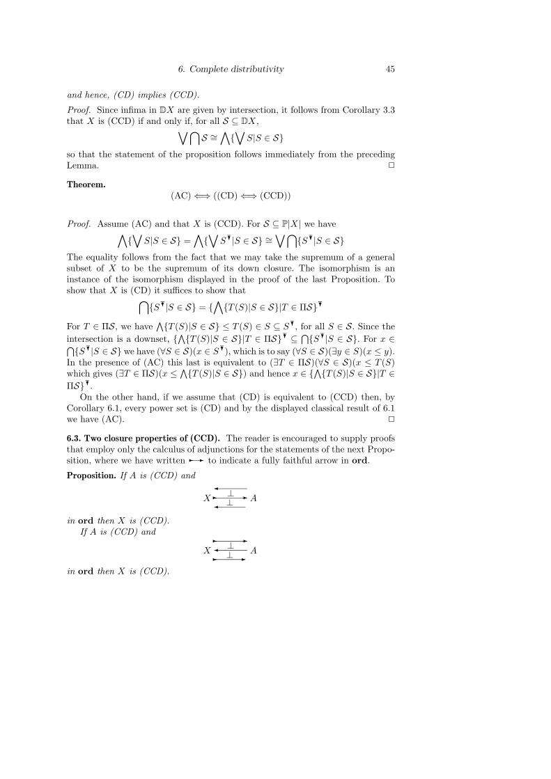
6. Complete distributivity 45

and hence, (CD) implies (CCD).

Proof. Since infima in DX are given by intersection, it follows from Corollary 3.3that X is (CCD) if and only if, for all S ⊆ DX,∨⋂

S ∼=∧∨S|S ∈ S

so that the statement of the proposition follows immediately from the precedingLemma. 2

Theorem.(AC)⇐⇒ ((CD)⇐⇒ (CCD))

Proof. Assume (AC) and that X is (CCD). For S ⊆ P|X| we have∧∨S|S ∈ S =

∧∨S ?|S ∈ S ∼=

∨⋂S ?|S ∈ S

The equality follows from the fact that we may take the supremum of a generalsubset of X to be the supremum of its down closure. The isomorphism is aninstance of the isomorphism displayed in the proof of the last Proposition. Toshow that X is (CD) it suffices to show that⋂

S ?|S ∈ S = ∧T (S)|S ∈ S|T ∈ ΠS?

For T ∈ ΠS, we have∧T (S)|S ∈ S ≤ T (S) ∈ S ⊆ S ?, for all S ∈ S. Since the

intersection is a downset, ∧T (S)|S ∈ S|T ∈ ΠS?⊆

⋂S ?|S ∈ S. For x ∈⋂

S ?|S ∈ S we have (∀S ∈ S)(x ∈ S ?), which is to say (∀S ∈ S)(∃y ∈ S)(x ≤ y).In the presence of (AC) this last is equivalent to (∃T ∈ ΠS)(∀S ∈ S)(x ≤ T (S)which gives (∃T ∈ ΠS)(x ≤

∧T (S)|S ∈ S) and hence x ∈

∧T (S)|S ∈ S|T ∈

ΠS ?.On the other hand, if we assume that (CD) is equivalent to (CCD) then, by

Corollary 6.1, every power set is (CD) and by the displayed classical result of 6.1we have (AC). 2

6.3. Two closure properties of (CCD). The reader is encouraged to supply proofsthat employ only the calculus of adjunctions for the statements of the next Propo-sition, where we have written -- to indicate a fully faithful arrow in ord.

Proposition. If A is (CCD) and

X A-- ⊥ ⊥

in ord then X is (CCD).If A is (CCD) and

--

X A ⊥-- ⊥

in ord then X is (CCD).

46 I. Ordered Sets

In the first diagram of the Proposition observe that the arrow from X to Apreserves all infima and all suprema. Such an arrow, between (antisymmetric) com-plete lattices, fully faithful or not, is sometimes called a complete homomorphism.When A in the first diagram is of the form PS, for S a set, and X is literally a sub-set of A, earlier terminology referred to X as a complete ring of sets. In the seconddiagram of the Proposition the arrow from A to X is surjective (for antisymmetricX and A) and in this case X is sometimes called a complete homomorphic imageof A.

Exercises.

1. Show that a complete ring of sets X --PS necessarily has X = D(S,≤) for a unique

order on S.2. For an adjoint sequence f a u a g in ord, show that f is fully faithful if and only if

g is fully faithful.3. For an adjoint sequence f a u a g in ord, with f , equivalently g, fully faithful, show

that f ≤ g.

6.4. The Raney-Buchi theorem. The following theorem, stated for (CD) lattices,was discovered independently by Raney and Buchi. Their classical result followsimmediately from the following constructive version using Theorem 6.2.

Theorem. An (antisymmetric) complete lattice is (CCD) if and only if it is acomplete homomorphic image of a complete ring of sets.

Proof. If X is (CCD) then by definition we have--⊥X DX⊥--↓

⊥

P|X|--⊥

which provides a presentation of the kind required. (The left adjoint to X DX :∨is necessarily fully faithful by Exercise 2 of 6.3.)Conversely, if we have

--⊥X R⊥ --

⊥

PS--⊥

for a set S then PS is (CCD) by Corollary 6.1, whereupon R is (CCD) by thefirst clause of Proposition 6.3 and finally X is (CCD) by the second clause ofProposition 6.3 2

6.5. The dual of (CCD). We say that X is (opCCD) if Xop is (CCD). We use(opCD) similarly and recall the classical result:

(AC) =⇒ ((opCD)⇐⇒ (CD))

We write (BLN) to indicate that set is further assumed to satisfy the Booleanaxiom.

Proposition. If (BLN) holds and X is (CCD) then X is (opCCD).

References 47

Proof. Apply (−)op (which provides a 2-functor (−)op : ordco -ord, see exer-cises 1 and 2 of 5.2) to the diagram

--⊥X DX⊥--↓

and obtain by Proposition 2.4 and the first Lemma in 5.5

--↓op

Xop (DX)op⊥-- ⊥

Now (DX)op = UXop and as pointed out immediately prior to the exercises in 5.2we always have pseudo-complementation (−)c : UX -

DX. In the case at hand,(BLN) gives an isomorphism (−)c : (DX)op '-DXop. Now DXop is in any event(CCD) and thus (BLN) implies that (DX)op is (CCD), whereupon the seconddisplay above and the second clause of Proposition 6.3 show that Xop is (CCD).

2

Since (−)op : ordco -ord is in any event an involutive isomorphism it is clearthat if (CCD) =⇒ (opCCD) then (CCD) ⇐⇒ (opCCD). Using the very specialproperty of Ω given in Theorem 4.1 we can expand on the last Proposition asfollows:

Theorem.(BLN)⇐⇒ ((CCD)⇐⇒ (opCCD))

Proof. It only remains to be shown that (BLN) follows from (CCD) =⇒ (opCCD).Since Ω ∼= P1 is in any event (CCD) the assumption ensures that Ωop is (CCD)and by Proposition 6.1 is thus Heyting. But we have seen in Theorem 4.1 thatwhen Ωop is Heyting Ω is Boolean. 2

Just as (AC) ensures the equivalence of (CD) and (CCD) so it also providesthe equivalence of (opCD) and (opCCD). Combining these equivalences with theclassical result that (AC) implies the equivalence of (CD) and (opCD), the Theoremabove provides a very indirect proof of Diaconescu’s Theorem:

Corollary.(AC) =⇒ (BLN)

References

[1] A. Carboni, S. Kasangian, and R. Street, Bicategories of spans and relations, J.Pure Appl. Algebra 33 (1984) 259–267.

[2] B. Fawcett and R. J. Wood, Constructive complete distributivity I, Math. Proc.Cam. Phil. Soc. 107 (1990) 81–89.

48 I. Ordered Sets

[3] P. T. Johnstone, Stone Spaces, Cambridge University Press, 1982.[4] P. T. Johnstone, Topos Theory, Academic Press, 1977.[5] F.W. Lawvere and R. Rosebrugh, Sets for Mathematics, Cambridge University

Press, 2001.[6] F. Marmolejo, R. Rosebrugh and R. J. Wood, A Basic Distributive Law, J. Pure

Appl. Algebra, to appear.[7] R. Rosebrugh and R. J. Wood, Constructive complete distributivity II, Math. Proc.

Cam. Phil. Soc. 110 (1991) 245–249.[8] R. Rosebrugh and R. J. Wood, Constructive complete distributivity IV, Applied

Categorical Structures 2 (1994) 119–144.[9] R. Rosebrugh and R. J. Wood, Boundedness and complete distributivity, Applied

Categorical Structures, to appear.[10] R. Street and R. F. C. Walters, Yoneda structures on 2-categories, Journal of

Algebra 50 (1978) 350–379.

Department of Mathematics and Statistics,Dalhousie University,Halifax NS B3H 3J5, CanadaE-mail : rjwood@mathstat.dal.ca