INSTITUTE OF PHYSICS PUBLISHING MEASUREMENT SCIENCE AND TECHNOLOGY

Meas. Sci. Technol. 12 (2001) 288–298 www.iop.org/Journals/mt PII: S0957-0233(01)17393-5

Measurement of surface tension andcontact angle using entropic edgedetectionC Atae-Allah1, M Cabrerizo-Vılchez1, J F Gomez-Lopera1,J A Holgado-Terriza1, R Roman-Roldan1 andP L Luque-Escamilla2,3

1 Departamento Fısica Aplicada, Universidad de Granada, Campus Fuente Nueva,18071 Granada, Spain2 Departamento Ingenierıas Mecanica y Minera, EUP Linares, Universidad de Jaen,C/Alfonso X el Sabio, 28, 23700 Linares (Jaen), Spain

E-mail: chakir0@yahoo.com (C Atae-Allah), mcabre@ugr.es (M Cabrerizo-Vılchez),jfgomez@ugr.es (J F Gomez-Lopera), jholgado@wanadoo.es (J A Holgado-Terriza),rroman@ugr.es (R Roman-Roldan) and peter@ujaen.es (P L Luque-Escamilla)

Received 25 September 2000, in final form 21 December 2000, accepted forpublication 3 January 2001

AbstractThis paper presents a new method to measure the surface tension and thecontact angle of a liquid. The measurement procedure comprises threesteps: acquisition of the liquid drop image, image segmentation to obtain thecontour of the drop and surface-tension and contact-angle calculation by theADSA method. In the second step a new segmentation method is used basedon the Jensen–Shannon divergence, an entropic measurement of coherenceamong distribution probabilities. The advantages of using this entropicedge-detection method are shown; it is especially suitable when the sourceimage of the drop is affected by any kind of noise, blur or low-contrast effect.Results reveal a better performance than other methods used in this field.

Keywords: surface tension, contact angle, Jensen–Shannon divergence, edgedetection, edge linking

1. Introduction

Surface tension is one of the most accessible experimentalparameters that describes the thermodynamic state andstructure of an interface. It is also of special interest in manydifferent fields in physics and engineering, such as lubricationin machinery, diffusion and migration of liquids throughporous media—very important in the search for oilfields,coatings, dispersions, adhesion, membranes etc. It is also veryimportant in the drop-formation process, which is fundamentalin industrial applications such as mixing, chemical processing,fibre spinning, silicon-chip technology and spraying (in ink-jetprinters, diesel motors and irrigation).

The Wilhelmy plate and the Nouy ring methods havetraditionally been used for surface-tension measurement [1, 2].These procedures are accurate but difficult to use, and muchcare must been taken in the measurement process. A new

3 All correspondence to be submitted to Pedro Luis Luque-Escamilla.

technique, called the drop-shape method, has been developedin recent years [3] taking advantage of new advances in imageprocessing. The drop-shape method operates by adjustinga theoretical contour to the drop border obtained by imagesegmentation. Commonly used drops are the sessile drop(formed on a surface) and the pendant drop (hanging froma capillary tube). This technique has some advantagesin comparison to traditional methods. First, only smallquantities of liquid are needed. Second, it can be appliedto liquid–vapour and liquid–liquid interfaces. Third, it canbe used in extreme conditions of temperature and pressure.Moreover, the interface is not contaminated or interfered withby the system. In addition, the technique makes it possibleto measure many parameters that cannot be obtained withtraditional methods, such as the dynamic interfacial tension,dynamic contact angle [3], film balance [4] etc.

The first numerical method to measure surface tensionwas established by Bashforth and Adams [5]. Since then,

0957-0233/01/030288+11$30.00 © 2001 IOP Publishing Ltd Printed in the UK 288

Image-based surface tension measurement

great improvements in the speed and accuracy of the methodhave been obtained with the introduction of computer imageanalysis. There is a vast bibliography that covers all thedifferent aspects of this topic: data acquisition, differentedge-detection methods to detect the drop profile, differentalgorithms of integration and optimization schemes [6–13].However, none of these methods is robust against noise inthe source-drop image. Moreover, the drop image must bewell focused and images obtained in practice are unfortunatelyfrequently noisy and out of focus, fundamentally due tothe acquisition procedure (CCD or photographic devices, forexample) [14]. The advantage of using the proposed entropicedge-detector method is its robustness when managing imagesaffected by these defects.

The paper is structured as follows. Section 1 introducesthe method. Section 2 reveals the technique of obtaining thesurface-tension value using the novel edge-detection methodproposed and an optimization algorithm to fit the detected dropshape to the theoretical one. Results are presented in section 3and the conclusions in section 4.

2. Surface-tension calculation method

The procedure for measuring the surface tension and contactangle of a liquid is a three-step one, described as follows.

Step 1. Image acquisition. In this step an image of theliquid drop is acquired from a CCD or photographic deviceand stored in digital form in a computer.

Step 2. Edge detection. In this stage an edge-detectionmethod is applied to find the drop contour in the image.It is usually recommendable to apply an edge-linkingalgorithm to ensure the closeness of the detected borders.

Step 3. Interfacial parameter determination. Oncethe experimental drop profile is performed, a numericalmethod is used to obtain the theoretical one that bestfits it. The interfacial parameters of the liquid drop canbe obtained from the knowledge of the fitted theoreticalprofile.

2.1. Image acquisition

The experimental apparatus for surface-tension measurementis shown in figure 1. As can be seen, it is comprised of twomain devices: the image-acquisition and drop-control systems(which controls the drop and environmental conditions).

A Leika Apozoom microscope coupled with a SonyCCD B&W video camera—SSC-M370CE with 752 × 582resolution—was used for the image acquisition. The camerais connected to a video frame-grabber card (DT 2855) thathas a resolution of 768 × 512 pixels with 256 grey levels.The frame-grabber card has a similar resolution to the videocamera, which prevents loss of accuracy in the light-intensitydetection of each photocell of the video camera. This feature isimportant for detecting the drop profile with the best possibleprecision. The frame-grabber board is mounted on a Pentiumcomputer and to a separate RGB monitor to display the drops.The light source is placed behind a diffuser that produces auniform light on the drop, which is controlled by a variacpower supply. To avoid vibration, all the instrument devices

are placed on an antivibratory table from Kinetic System Inc.Vibraplane. The drop is put into a glass cuvette, inserted intoa thermostatted cell, which maintains a constant temperaturevalue by water circulation through a jacket. The cell is on athree-axis micropositioner that allows the drops to be handledin any direction.

In pendant experiments, the drop is inserted into the cellwith a syringe (Hamilton Microlab 500 microinjector) thatpulls the liquid into a Teflon capillary 0.5 mm in diameterthat prevents wetting of the liquid. This allows the formationof stable drops automatically at low injection rate to preventdrop vibration. In sessile experiments, the drop is placed on thesurface with a microsyringe that controls the amount of liquidinserted. For sessile experiments a solid surface with a lowsurface tension was chosen (Teflon (FEP)). The microsyringeis attached to a stand adapter to minimize vibration. Allglassware and Teflon ware were cleaned in chromic sulphuricacid.

First of all, instrument calibration is necessary to obtainaccurate and precise surface-tension values. A plumb bob isused to align the vertical axis with the vertical axis of the videocamera because the drop must be axisymmetric in order to usethe optimization method in section 2.3. The plumb consists of aweight hanging from a fine copper wire submerged in a beakerof water to dampen oscillations. An image of the plumb wireis captured with the CCD camera and a program determinesthe vertical axis. This process continues until the user correctsthe vertical axis of the video camera. A grid with an arrayof squares of 0.25 mm per side (Graticules Ltd Tonbridge) isused to determine the picture magnification, horizontal/verticalaspect ratio and geometric distortion due to the optical system.The program uses the grid to calculate the co-ordinates ofthe drop profile extracted with the edge-detection method inmillimetres.

2.2. Edge detection

In the specialized literature, detection of drop profiles isusually performed using both global and adaptive thresholdingmethods [6–8]. These techniques require highly contrastedimages to select the right threshold value, so they are onlyadequate for pendant drops in a liquid–vapour interface.Sessile and pendant drops in liquid–liquid interfaces have suchpoor contrast in general that it is not easy to obtain the dropprofile with these traditional methods. This is why [9, 13] usemore powerful edge detectors, based on gradient magnitudes,such as Sobel or five-level Robinson detectors [14].

In addition, many causes can degrade the image duringthe acquisition process:

(a) uncertainties in the sensor, fluctuations in the lightintensity, and other similar error sources;

(b) photoelectronic, Gaussian noise appearing in theconversion of photons to electrons;

(c) thermal noise in the signal amplification process—usuallythis kind of noise is modelled as Gaussian type, with zeromean;

(d) impulsive type noise (salt and pepper) appearing in signaltransmission processes and

(e) other causes of error (blur due to drop vaporization, outof focus etc).

289

C Atae-Allah et al

Figure 1. Schematic illustration of drop-shape method.

Unfortunately, none of the edge-detection techniquescommonly used in the specialized literature is robust againstnoise or blurring. The method presented in this paper,in contrast, is applicable in any practical situation, evenwhen the above-mentioned defects appear. It is basedon the Jensen–Shannon divergence between the normalizedhistograms of two samples taken from the image.

2.2.1. The Jensen–Shannon divergence. Jensen–Shannondivergence (hereafter JS), proposed by Lin [15], has proved tobe a powerful tool in the segmentation of digital images [16].It is a measurement of the inverse cohesion of a set ofprobability distributions having the same number of possiblerealizations:

JSπ (P1, P2, . . . , Pr) ≡ H

( r∑i=1

πiPi

)−

i∑i=1

πiH(Pi) (1)

where

P1, P2, . . . , Pr are discrete probability distributions

Pi == {Pi,j /j = 1, . . . , n} i = 1, . . . , r

π1, π2, . . . , πr are the distribution weights for Pi;

π ≡{π1, π2, . . . , πr/πi > 0,

r∑i=1

πi = 1

}

H(Pi) = −n∑

j=1

Pi,j logPi,j is the Shannon entropy.

Divergence grows as the differences between its argu-ments (the probability distributions involved) increase, andvanishes when all the probability distributions are iden-tical. As only two probability distributions are usedhere, the final expression of the Jensen–Shannon divergenceis

JS(P1, P2) ≡ H

(P1 + P2

2

)− 1

2[H(P1) + H(P2)]. (2)

The application of JS to edge detection is based on a three-stepstructured procedure, as follows [17].

(a) Calculation of divergence and direction matrices. Inthis step the divergence and direction matrices associatedwith the image are calculated. The divergence matrix iscomposed of real numbers and is similar to that obtainedwith the gradient operator for edge detection. Thedirection matrix contains the estimated edge direction forall image pixels.

Figure 2. A window sliding across a perfect edge.

(b) Edge-pixel selection. Edge pixels are chosen by means ofa local maximum selection criterion from the divergencematrix, resulting in a binary image with the image edges.

(c) Edge linking. The final stage is an edge-prolongationprocedure that attempts to connect sets of unconnectededge pixels in the previously obtained binary image.

2.2.2. Calculation of divergence and direction matrices. Letus consider a window made up of two identical subwindowsand sliding down over a straight edge between two differenttextures (see figure 2). It has been shown [16] that insuch conditions the JS between the normalized histogramsof the subwindows reaches its maximum value when eachsubwindow lies completely within one texture.

In accordance with the above procedure, it is possible toassign a JS value to each pixel in the image. Hence, pixelswith a high JS have a high probability of being edge pixels,and vice versa. If, unlike the example shown in figure 2,the window-to-edge angle is not 90◦, the JS maximum willbe low or even undetectable, while the JS inside a giventexture will be close to zero or to the base value. This thenmeans trying several window orientations for each pixel. Onlyfour orientations are, however, technically possible: vertical,horizontal, and two diagonals. Thus, the values JS1, JS2, JS3

and JS4 are calculated for the fixed window orientations 0,π/4,π/2 and 3π/4. In this work we have used a square slidingwindow, with user-defined size.

Now the question is how to obtain an estimate of thedirection from these four values that maximizes the JS and thenthe value of this maximum, JSmax . For a given pixel, the JSvalue is a π -periodic function of window orientation over theimage. It reaches its maximum value for a given orientation,β, and a minimum in β + π . A theoretical model describingthis periodic function can thus be expressed as follows:

JS(x) = a + b cos(β + 2πx) x ∈ [0, 1] (3)

290

Image-based surface tension measurement

where a and b are constants determining the amplitude of JSoscillation and β ∈ [0, π) is the edge direction in this pixel.The JS direction, x, is normalized in the interval [0, 1] tosimplify calculations. According to the trigonometric relation,a theoretical model equivalent to (3) is

JS(x) = c + msen(2πx) + n cos(2πx) x ∈ [0, 1] (4)

where c, m and n are constants. Nevertheless, due to thecomputational effort required for trigonometric functions, theycan be replaced by other functions with similar properties, suchas quadratic splines:

sen(2πx) ≈ f (x) ≡{−16x2 + 8x x ∈ [0, 1

2 ]

16x2 − 24x + 8 x ∈ [ 12 , 1]

cos(2πx) ≈ g(x)

≡

−16x2 + 1 x ∈ [0, 1

4 ]

16x2 − 16x + 3 x ∈ [ 14 ,

34 ]

−16x2 + 32x − 15 x ∈ [ 34 , 1].

(5)

Then, f (x) is obtained as a quadratic spline of class 1, withnodes at points {0, 1

4 ,12 ,

34 , 1}, interpolating to sen(2πx) at

points {f (0), f ( 14 ), f (

12 ), f (

34 ), f (1), f

′( 14 ), f

′( 34 )}. In the

same way, g(x) is obtained as a quadratic spline of class 1with the same nodes as f (x), interpolating to cos(2πx) atthe points {g(0), g( 1

4 ), g(12 ), g(

34 ), g(1), g

′(0), g′( 12 ), g

′(1)}.With a least-squares fit of the divergence model (4) and themodification (5) for points JS1, JS2, JS3 and JS4, the solutionis

JS(x) = JS1 + JS2 + JS3 + JS4

4+

JS2 − JS4

2f (x)

+JS1 − JS3

2g(x). (6)

The direction, x, having the maximum JS values can beobtained from the equations

if JS1 − JS3 � 0, JS2 − JS4 � 0⇒x = JS2 − JS4

4[(JS1 − JS3)− (JS2 − JS4)]∈ [0, 1

4 ]

if JS1 − JS3 � 0, JS2 − JS4 � 0⇒x = 4(JS1 − JS3)− 3(JS2 − JS4)

4[(JS1 − JS3)− (JS2 − JS4)]∈ [ 3

4 , 1]

if JS1 − JS3 � 0, JS2 − JS4 � 0⇒x = 2(JS1 − JS3)− (JS2 − JS4)

4[(JS1 − JS3)− (JS2 − JS4)]∈ [ 1

4 ,12 ]

if JS1 − JS3 � 0, JS2 − JS4 � 0⇒x = 2(JS1 − JS3) + 3(JS2 − JS4)

4[(JS1 − JS3)− (JS2 − JS4)]∈ [ 1

2 ,34 ]. (7)

Finally, defining δ = πx ∈ [0, π) as the estimated edgedirection, the method described above calculates x from (7)(i.e., the estimated direction that maximizes the JS) and theestimated JSmax from (6).

In this way, each image pixel is labelled with a pair ofvalues: the estimated edge direction and the estimated JSmax

placing the sliding window in accordance with the estimatededge direction. Thus, two matrices are built: the divergencematrix (which indicates the probability of a pixel belonging tothe image edge) and the direction matrix (which estimates theedge direction for the edge pixels).

Estimated edgedirection

Sliding monodimensional window

Pixel under study

Figure 3. Monodimensional window, perpendicular to estimateddirection in each image pixel.

However, direct application of the above method doesnot provide good results for some kinds of image—corruptedby Gaussian noise, or with regions having small fluctuationsin grey levels—because the JS could be too sensitive to anychange in grey levels between regions. It is therefore betterto construct the divergence matrix including extra informationin addition to the histogram information using the followingexpression:

JS∗i,j = JSi,j (1− α + αWi,j ) (8)

where Wi,j = |Nw1 − Nw2|/Nw, Nw1 and Nw2 being theaverage grey levels of subwindows W1 and W2, and Nw themaximum grey level inside the window (normalization factor).α ∈ [0, 1] is the attenuation factor, which determines theweights of JS and the grey levels inside the window. Thismodification makes the JS suitable for different kinds of image,thus transforming our algorithm into a hybrid among texture-based algorithms [18], Jensen–Shannon divergence [16] andgrey-level based algorithms (gradient, Laplacian, Laplacianand gradient of the Gaussian etc) [19–21].

2.2.3. Edge-pixel selection. In this step the procedureselects which pixels from the divergence matrix are edgepixels. Thresholding the divergence matrix [22] is not alwaysuseful, since maximum JS values depend on the compositionof adjacent textures, and will thus vary according to texture.Consequently, it would seem more appropriate to use a localcriterion. Accordingly, each edge-pixel candidate is thecentre of an odd-length monodimensional window, placedperpendicular to the estimated edge direction in that pixel(figure 3).

Thus, every edge pixel has to satisfy

JScentre − JSj � Td (9)

for any other pixel j in that particular monodimensionalwindow, where Td is a threshold. Pixels marked as edge pixelsare then outstanding local maxima of the divergence matrix.Obviously, detection results depend directly on the parameterTd , which can be modified by the user if necessary.

This local edge-pixel detection method requires simpledivergence matrix pre-processing. Small fluctuations, oftendue to noise in the original image or to texture regularity,can introduce a great number of false maxima, although theyare usually fairly low. The divergence matrix is thereforesmoothed out by repeatedly applying a 3× 3 mean filter.

Selection of a local maximum is, in a sense, a thinningprocedure since just one pixel will usually be detected as an

291

C Atae-Allah et al

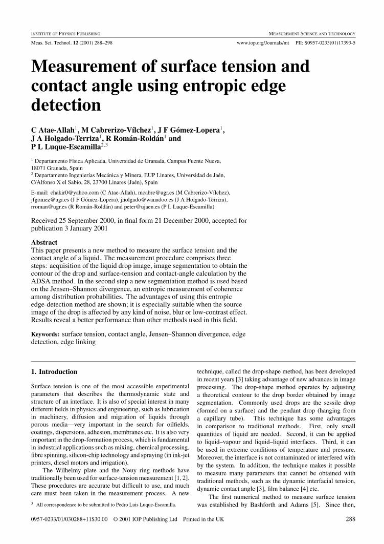
C C C C C C

E C E C E

C

Figure 4. End points and neighbour candidates for edgeprolongation. E, end point; C, neighbour candidates. The remaininggrey pixels are edge pixels.

edge pixel within the neighbourhood, as determined by the sizeof the monodimensional window. In fact, rarely would morethan one pixel share the same maximum JS.

2.2.4. Edge linking. The two steps described above makeit possible to extract the image edge pixels. However, it isnot always feasible to establish a good compromise betweenthe quality of the binary image obtained and the desiredconnectivity of the edge pixels, possibly due to the presenceof noise in the original image, and the texture composition ofthe image regions.

In order to deal with these problems, a third step canbe added: edge-pixel linking [23]. This step attempts tojoin the various sets of edge pixels using information fromthe divergence matrix associated with the image, togetherwith knowledge of the direction in which maximum JS isproduced. In broad terms, the linking procedure consists inextracting edge pixels unmarked since they did not satisfythe condition (9), but nearly did. Not all the pixels in theimage are candidates for filling the gaps, only those classifiedas neighbour candidates of end pixels.

The definition of end pixel in [24] includes several variantsthat may influence the result of the linking process. Thepresent paper uses the definition of end pixel as a pixelhaving one or two marked pixels joined together. Thus, onlycertain neighbour end pixels are candidates for prolongingimage edges. In figure 4 we present the candidate pixels forcontinuing a given edge.

For a given neighbour candidate to be marked as an edgepixel, it must satisfy two conditions:

(a) Its associated JS must be reasonably high. The firstprolongation condition is then

JSend − JSneighbour candidate � τd (10)

where τd is a threshold, which has at first no relation withparameter Td in step (2) of the procedure.

(b) The estimated edge direction of the end pixel (Dirend), theedge-direction neighbour candidate (Dirneighbour candidate)and the direction of the physical line joining them (Dir(end, neighbour candidate)) must not differ by more thana specified amount. The second prolongation condition isthen

(Dir (end, neighbour candidate))-Dirend)2

+(Dir (end, neighbour candidate)

−Dirneighbour candidate)2 � τθ (11)

where τθ is another threshold.

Table 1. Typical parameter values.

Parameter value Typical value

Step 1 1. Sliding window size 3× 32. Attenuation coefficient 0.75

Step 2 1. Monodimensional window size 112. Mean filter iterations 83. Local maximum selection threshold 0.7

Step 3 1. Divergence threshold 0.12. Direction threshold 0.5

The two foregoing conditions are used in an attempt toextract as edge pixels those pixels lying next to end pixels andwhose JS and direction are sufficiently close to those of the endpixel to be extended. It should be borne in mind that when anew pixel is marked as an edge, other adjacent pixels can thenbecome end pixels. So, the algorithm must foresee this eventin order to continue the search for links.

2.2.5. Final considerations about edge-detection procedure.This section briefly summarizes all the parameters used by theedge-detection procedure. Initially, the proposed segmentationprocedure may seem difficult to use due to the elevated numberof parameters that user can vary. But in practice the procedureis easy to use because all the images are similar. In table 1 wepresent the typical parameter values used in this work.

2.3. Interfacial-parameter determination

Once the profile of the drop is obtained, a numerical method isused for obtaining the theoretical profile of the drop that bestfits it by adjusting the interfacial parameters, which are thendetermined.

The theoretical profile determination of a liquid drop isa complex problem. From equilibrium considerations, Youngand Laplace concluded that

�P = γ

(1

R1+

1

R2

)(12)

where �P is the pressure difference across the interfacebetween the two phases (liquid–gas or liquid–liquid), γ is thesurface tension and R1 and R2 are the two principal radii ofthe curvature of the drop surface. If the drop is axisymmetricwith respect to the vertical axis, the pressure difference in theapex of the drop �Pa can be calculated from equation (12) bytaking R1 = R2 = R0:

�Pa = 2γ

R0. (13)

Thus, �P in equation (12) may be put in terms of �Pa byusing the hydrostatic fundamental equation

�P = �Pa ±�ρgz = 2γ

R±�ρgz (14)

where ± means that the sum is carried out when the drop islying on a horizontal surface (sessile drop) and the difference istaken when the drop is falling from a dropper (pendant drop);�ρ is the density difference between liquid and surrounding

292

Image-based surface tension measurement

0

Φ

s

soyo

xo

y

x

0x

y

φ

φ φ

s

R1

s

yo

xo

R2

Figure 5. Definition of co-ordinate systems in pendant and sessile drops.

gas, to take into account Archimedes’ buoyancy; g is thegravity acceleration where the measurements were performedand z is the height above (or below) the apex.

In order to obtain the differential equations describingthe drop profile, hydrostatic equilibrium considerations, or avariational approach—such as a minimization of the sum ofthe gravitational and surface potential energies [25]—can betaken. These equations are [10]

dx

ds= cosφ

dy

ds= sin φ

dφ

ds= 2

R− sin φ

r± �ρgy

γ(15)

where the angles and lengths are shown in figure 5.This set of equations can be integrated simultaneously, in

function of parameter s, using a numerical procedure suchas a fourth-order Runge–Kutta scheme [12] or the second-order implicit Euler method [10]. The theoretical profileof the drop for a given R0, g, �p and γ is then obtained.The initial values required to start the integration process arex(s = 0) = y(s = 0) = φ(s = 0) = 0.

Several optimization methods have been developed to fitthe theoretical drop profile to the experimental one [8, 12]. Inthis work, the ADSA (axisymmetric drop shape analysis) [10]method has been chosen, because it offers better solutions overa wide range of situations, in addition to being used by somelaboratories [26–28]. This algorithm is described below.

A number of points in the drop-image border are taken andthen the theoretical drop shape is fitted to them by minimizingthe Euclidean distance, d(·, ·), between the empirical pointsun and the theoretical profile points, v, obtained fromequation (15). The objective function to optimize is

E = 1

2

N∑n=1

[d(un, v)]2 (16)

where N is the number of empirical points taken fromthe border image of the drop. The change in d(·, ·) isachieved by modifying the interface parameters and thenthe theoretical profile. Minimization is performed using theNewton–Rhapson method, which converges to the optimalvalue. However, initial values are required to use the method.

3. Experimental results

2-propanol (grade 99.5+%) from Sigma Aldrich andformamide (grade 99+%) from Carlo Erba Reagents were usedto carry out the surface-tension calculation with the proposedmethod. Robinson and Sobel edge-detector results, which arecommonly employed in this kind of problem [9, 13], are alsoincluded for comparison.

Some reference values of the calculated parameters aregiven to show the accuracy of the results. The referencevalue for surface tension of 2-propanol is 23.32 mJ m−2 at25 ◦C [29]. The formamide surface-tension reference value is57.49 mJ m−2, and the contact angle is 95.38◦ [30], both at20 ◦C.

3.1. Experimental data and analysis

In this section the results of surface-tension and contact-angle determination for real drop images are presented. Theinterfacial parameters were calculated by the ADSA methodin all cases.

The first experiments correspond to the interfacialparameter determination of drop images unaffected by bluror noise. From a set of eight 2-propanol pendant drops,we obtained surface-tension values of 24.06 ± 0.33 mJ m−2

(Sobel), 24.17 ± 0.26 mJ m−2 (Robinson) and 24.07 ±0.27 mJ m−2 (JS), whereas from six sessile drops of formamidethe results are 57.1± 4.5 mJ m−2 (Sobel), 58.0± 4.2 mJ m−2

(Robinson) and 57.3 ± 4.9 mJ m−2 (JS). The contact anglevalues in this later case are 96.8 ± 1.8 (Sobel), 96.8 ± 4.6(Robinson) and 97.4±2.2 (JS). Error estimation in all the abovedata is the 95% confidence interval (1.96σ/

√N ) assuming

the errors follow a Gaussian model. From the experimentalresults we can observe that the ADSA method using JS canprovide results as accurate as those using traditional Sobel andRobinson edge detectors when applied to clean—unaffectedby noise or blur—drop images.

With respect to formamide, note that the experimentalmean values are slightly different to the reference values(shown in table 3), although the error intervals include thelatter. A high discrepancy in the error interval of the interfacialparameters was obtained for the sessile drops compared withthe pendant experiment due to several reasons [3]. First,the sessile drops are very sensitive to the roughness andheterogeneity of the Teflon, thus causing a lack of vertical

293

C Atae-Allah et al

a)

b)

c)

d)

e)

f)

g)

Figure 6. Results of edge-detection in blurred images: (a) image of 2-propanol, blurred eight times; (b) the same as (a) for formamide; (c)and (d) results of segmenting images (a) and (b) with the Sobel edge-detector; (e) and (f ) the same as (c) and (d), applying the Robinsonedge-detector; (g) and (h) the same as (c) and (d), applying the JS edge-detector.

symmetry, which has a negative impact on the ADSA method.Second, a minimal variation in the drop size causes a changein the curvature of the drop that produces a variation in theinterfacial measurements. Third, the accurate determinationof the contact point can be difficult when the image has a low

contrast, such as in this case. A good contrast between the dropand the surface is extremely important for precise measurementof the interfacial parameters.

However, the real advantage of the proposed edge-detectormethod occurs in the application to noisy or blurred drop

294

Image-based surface tension measurement

a)

b)

c)

d)

e)

f)

g)

h)

Figure 7. Results of edge-detection with Gaussian noisy images (zero mean, standard deviation 15): (a) image of 2-propanol with Gaussiannoise; (b) the same as (a) for formamide; (c) and (d) results of segmenting images (a) and (b) with the Sobel edge-detector; (e) and (f ) thesame as (c) and (d), applying the Robinson edge-detector; (g) and (h) the same as (c) and (d), applying the JS edge-detector.

images. Thus, a set of real drop images, into which variousdegrees and types of noise have been introduced, are consid-ered in a second group of experiments. These experimentsare important for two reasons: they can simulate experimentalconditions that commonly appear in practice and they allow us

to evaluate the robustness of these edge-detection methods.Table 2 shows the numerical results of surface tension

using the Sobel, Robinson and JS methods. The original2-propanol pendant drop is contaminated with three syntheticdistortions (blur, and Gaussian and impulsive noise) to simulate

295

C Atae-Allah et al

(a) (b)

(c) (d)

(e) (f )

(g) (h)

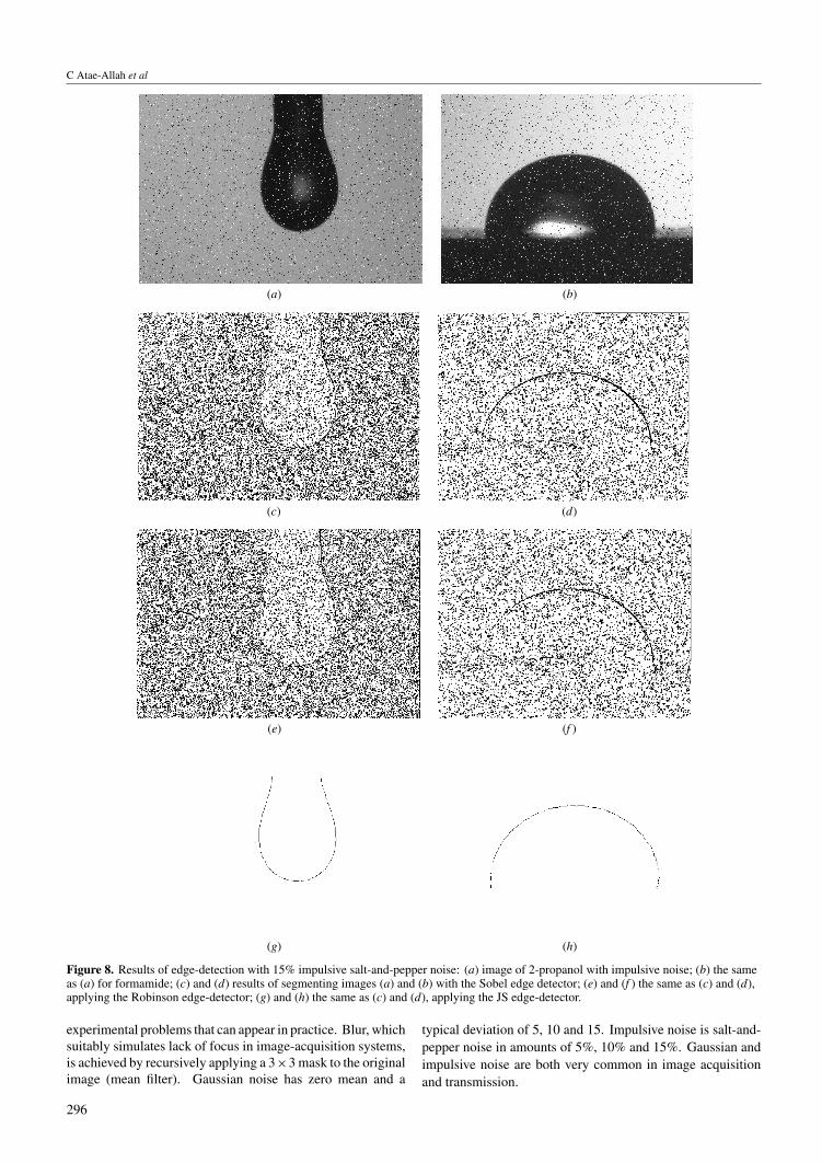
Figure 8. Results of edge-detection with 15% impulsive salt-and-pepper noise: (a) image of 2-propanol with impulsive noise; (b) the sameas (a) for formamide; (c) and (d) results of segmenting images (a) and (b) with the Sobel edge detector; (e) and (f ) the same as (c) and (d),applying the Robinson edge-detector; (g) and (h) the same as (c) and (d), applying the JS edge-detector.

experimental problems that can appear in practice. Blur, whichsuitably simulates lack of focus in image-acquisition systems,is achieved by recursively applying a 3×3 mask to the originalimage (mean filter). Gaussian noise has zero mean and a

typical deviation of 5, 10 and 15. Impulsive noise is salt-and-pepper noise in amounts of 5%, 10% and 15%. Gaussian andimpulsive noise are both very common in image acquisitionand transmission.

296

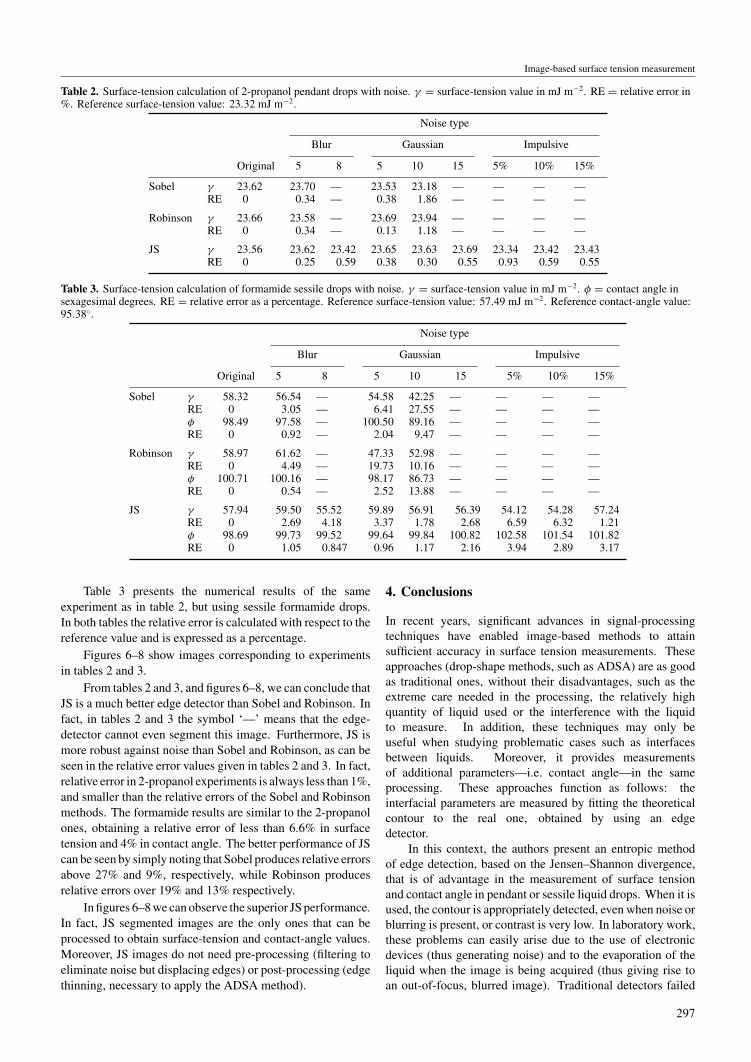
Image-based surface tension measurement

Table 2. Surface-tension calculation of 2-propanol pendant drops with noise. γ = surface-tension value in mJ m−2. RE = relative error in%. Reference surface-tension value: 23.32 mJ m−2.

Noise type

Blur Gaussian Impulsive

Original 5 8 5 10 15 5% 10% 15%

Sobel γ 23.62 23.70 — 23.53 23.18 — — — —RE 0 0.34 — 0.38 1.86 — — — —

Robinson γ 23.66 23.58 — 23.69 23.94 — — — —RE 0 0.34 — 0.13 1.18 — — — —

JS γ 23.56 23.62 23.42 23.65 23.63 23.69 23.34 23.42 23.43RE 0 0.25 0.59 0.38 0.30 0.55 0.93 0.59 0.55

Table 3. Surface-tension calculation of formamide sessile drops with noise. γ = surface-tension value in mJ m−2. φ = contact angle insexagesimal degrees. RE = relative error as a percentage. Reference surface-tension value: 57.49 mJ m−2. Reference contact-angle value:95.38◦.

Noise type

Blur Gaussian Impulsive

Original 5 8 5 10 15 5% 10% 15%

Sobel γ 58.32 56.54 — 54.58 42.25 — — — —RE 0 3.05 — 6.41 27.55 — — — —φ 98.49 97.58 — 100.50 89.16 — — — —RE 0 0.92 — 2.04 9.47 — — — —

Robinson γ 58.97 61.62 — 47.33 52.98 — — — —RE 0 4.49 — 19.73 10.16 — — — —φ 100.71 100.16 — 98.17 86.73 — — — —RE 0 0.54 — 2.52 13.88 — — — —

JS γ 57.94 59.50 55.52 59.89 56.91 56.39 54.12 54.28 57.24RE 0 2.69 4.18 3.37 1.78 2.68 6.59 6.32 1.21φ 98.69 99.73 99.52 99.64 99.84 100.82 102.58 101.54 101.82RE 0 1.05 0.847 0.96 1.17 2.16 3.94 2.89 3.17

Table 3 presents the numerical results of the sameexperiment as in table 2, but using sessile formamide drops.In both tables the relative error is calculated with respect to thereference value and is expressed as a percentage.

Figures 6–8 show images corresponding to experimentsin tables 2 and 3.

From tables 2 and 3, and figures 6–8, we can conclude thatJS is a much better edge detector than Sobel and Robinson. Infact, in tables 2 and 3 the symbol ‘—’ means that the edge-detector cannot even segment this image. Furthermore, JS ismore robust against noise than Sobel and Robinson, as can beseen in the relative error values given in tables 2 and 3. In fact,relative error in 2-propanol experiments is always less than 1%,and smaller than the relative errors of the Sobel and Robinsonmethods. The formamide results are similar to the 2-propanolones, obtaining a relative error of less than 6.6% in surfacetension and 4% in contact angle. The better performance of JScan be seen by simply noting that Sobel produces relative errorsabove 27% and 9%, respectively, while Robinson producesrelative errors over 19% and 13% respectively.

In figures 6–8 we can observe the superior JS performance.In fact, JS segmented images are the only ones that can beprocessed to obtain surface-tension and contact-angle values.Moreover, JS images do not need pre-processing (filtering toeliminate noise but displacing edges) or post-processing (edgethinning, necessary to apply the ADSA method).

4. Conclusions

In recent years, significant advances in signal-processingtechniques have enabled image-based methods to attainsufficient accuracy in surface tension measurements. Theseapproaches (drop-shape methods, such as ADSA) are as goodas traditional ones, without their disadvantages, such as theextreme care needed in the processing, the relatively highquantity of liquid used or the interference with the liquidto measure. In addition, these techniques may only beuseful when studying problematic cases such as interfacesbetween liquids. Moreover, it provides measurementsof additional parameters—i.e. contact angle—in the sameprocessing. These approaches function as follows: theinterfacial parameters are measured by fitting the theoreticalcontour to the real one, obtained by using an edgedetector.

In this context, the authors present an entropic methodof edge detection, based on the Jensen–Shannon divergence,that is of advantage in the measurement of surface tensionand contact angle in pendant or sessile liquid drops. When it isused, the contour is appropriately detected, even when noise orblurring is present, or contrast is very low. In laboratory work,these problems can easily arise due to the use of electronicdevices (thus generating noise) and to the evaporation of theliquid when the image is being acquired (thus giving rise toan out-of-focus, blurred image). Traditional detectors failed

297

C Atae-Allah et al

when trying to provide any measurement of the interfacialparameters in such situations.

The advantages of the Jensen–Shannon divergencedetector are due to its intrinsic properties of noise robustness[17]. When contrast is low, it is possible to include a refinementin the algorithm, named attenuation, thus making it capable ofdistinguishing the edges even in such a situation [31].

The Jensen–Shannon method provides the best resultswhen it is used with small windows since the observation levelis the more accurate [17]. It must be said that the edge linkingis essential in the results obtained, because only a few edgepixels are detected directly, due to the extreme conditions inwhich the algorithm has to work. This makes it necessaryto adjust the parameters in the detector to obtain a few edgepixels, but with a very high confidence level.

To sum up, the proposed Jensen–Shannon divergence edgedetector is very suitable for use in drop-shape methods for de-termining surface tension or contact angle in liquids, especiallywhen the quality of the drop images is relatively poor.

Acknowledgments

This work has been partially supported by grants MAR-97-0464 and MAT-98-0937-C02-C01 of the Spanish Government.Our thanks to Christine Laurin for revising the English.

References

[1] Weser C 1980 Measurement of interfacial tension and surfacetension—general review for practical man GIT Fachz.Laboratorium 24 642–8

Weser C 1980 Measurement of interfacial tension and surfacetension—general review for practical man GIT Fachz.Laboratorium 24 734–42

[2] Adamson A W 1982 Physical Chemistry of Surfaces (NewYork: Wiley)

[3] Neumann A W and Spelt J K 1996 Applied SurfaceThermodynamics (New York: Dekker)

[4] Kwok D Y, Vollhardt D, Miller R, Li D and Neumann A W1994 Axisymmetric drop shape analysis as a film balanceColloids Sufaces 88 51–8

[5] Bashforth F and Adams J C 1893 An Attempt to Test theTheories of Capillary Action (Cambridge: CambridgeUniversity Press)

[6] Girault H, Schiffrin D J and Smith B J 1984 The measurementof interfacial tension of pendant drops using a video imageprofile digitizer J. Colloid Interface Sci. 101 257–66

[7] Hansen F K and Rodsrud G 1991 Surface tension by pendantdrop J. Colloid Interface Sci. 141 1–9

[8] Anastasiadis S H, Chen J K, Koberstein J T, Siegel A F,Sohn J E and Emerson J A 1989 The determination ofinterfacial tension by video image processing of pendantfluid drops J. Colloid Interface Sci. 119 55–66

[9] Cheng P, Li D, Boruvka L, Rotenberg Y and Neumann A W1990 Automation of Axisymmetric drop shape analysis formeasurement of interfacial tensions and contact anglesColloids Surf. 43 151–67

[10] Rotenberg Y, Boruvka L and Neumann A W 1983Determination of surface tension and contact angle from theshapes of axisymmetric fluid interfaces J. Colloid InterfaceSci. 93 169–83

[11] Hansen F K 1993 Surface tension by image analysis: fast andautomatic measurements of pendant and sessile drops andbubbles J. Colloid Interface Sci. 160 209–17

[12] Huh C and Reed R L 1983 A method for estimating interfacialtensions and contact angles from sessile and pendant dropshapes J. Colloid Interface Sci. 91 472–84

[13] Pallas N R and Harrison Y R 1990 An automated drop shapeapparatus and the surface tension of pure water ColloidsSurf. 43 169–94

[14] Pitas G and Venetsanopoulos A N 1990 Nonlinear DigitalFilters (Dordrecht: Kluwer)

[15] Lin J 1991 Divergence measures based on the Shannonentropy IEEE Trans. Information Theory 37 145–50

[16] Barranco-Lopez V, Luque-Escamilla P L and Roman-RoldanR R 1995 Entropic texture-edge detection for imagesegmentation Electron. Lett. 31 867–69

[17] Gomez-Lopera J F, Robles-Perez A M, Martınez-Aroza J andRoman-Roldan R 2000 An analysis of edge detection byusing the Jensen–Shannon divergence J. Math. ImagingVision 13 35–56

[18] Park D J, Nam K M and Park R H 1994 Edge-detection innoisy images based on the co-occurrence matrix PatternRecognition Lett. 27 765–75

[19] Pratt W 1991 Digital Image Processing (New York:Wiley–Interscience)

[20] Marr D and Hildreth E 1980 Theory of edge detection Proc. R.Soc. B 207 187–217

[21] Canny J 1986 A computational approach to edge detectionIEEE Trans. Pattern Anal. Machine Intell. 8 679–98

[22] Barranco Lopez V, Luque Escamilla P L, Martınez Aroza Jand Roman Roldan R R 1995 Texture segmentation basedon information-theoretic edge detection method Proc. 6thSpanish Symp. on Pattern Recognition (Cordoba) pp 58–64

[23] Farag A A 1995 Edge linking by sequential search PatternRecognition 28 611–33

[24] Lam L 1992 Thinning methodologies—a comprehensivesurvey IEEE Trans. Pattern Anal. Machine Intell. 14 869–85

[25] Behroozi F, Macomber H K, Dostal J A and Behroozi C H1996 The profile of a dew drop Am. J. Phys. 64 1120–5

[26] Noordmans J and Busscher H J 1991 The influence of dropletvolume and contact angle on liquid surface tensionmeasurements by axisymmetric drop shape analysis-profile(ADSA-P) Colloid Surf. 58 239–49

[27] Lin S Y, Chen L J, Xyu J W and Weng W J 1995 Anexamination on the accuracy of interfacial tensionmeasurement from pendant drop profile Langmuir 114159–66

[28] Li D, Cheng P and Neumann A W 1992 Contact anglemeasurement by axisymmetric drop shape analysis Adv.Colloid Interface Sci. 39 342–82

[29] Li D and Neumann A W 1992 Contact angles of binary liquidsand their interpretation J. Adhesion Sci. Technol. 6 601–10

[30] Li D and Neumann A W 1992 Contact angles of hydrophobicsolid surfaces and their interpretation J. Colloid InterfaceSci. 148 190–200

[31] Holgado Terriza J A, Gomez Lopera J F, Luque Escamilla P L,Atae-Allah C and Cabrerizo-Vılchez M 1999 Measurementof ultralow interfacial tension with ADSA using an entropicedge-detector Colloids Surf. A 156 579–86

298