I) Resistivity

Literatur:

• Telford, Geldart und Sheriff (1990): Applied Geophysics, Second Edition, Cambridge University Press, NY.

• Bender, F. (Hg.) (1985): Angewandte Geowissenschaften, Bd. II, Enke Verlag, Stuttgart.

Specific resistivity of rocks:

• most minerals form isolators (z.B. NaCl - ). • given some amount of water the apparent resistivity changes dramatically. Sediments

resistivity values: ; granite and metamorphic rocks:

The resistivity of rocks with no clay content can be expressed by Archie’s law:;

specific resistivity; A amount of pore fluid; F formation factor (depends on the total volume of porosity) resistivity of pore fluid

large bandwidth of resistivity values for different rocks (partially overlapping) without further geological knowledge no unique interpretation possible

106Ωm

5 1000Ωm– 100 105Ωm–

ρ AFρw=

ρ

ρw

⇒⇒

1) Basic physical relations

In 1860 James Clerc Maxwell founded the complete theory of electromagnetic properties:

; ; ;

;

H magnetic field strength; B magnetic induction; E electric field strength; D electric displacement; j electric current density; q space charge density,

Nablaoperator.

∇ H× rotH j t∂∂D+= = ∇ E× rotE t∂

∂B–= = ∇B divB 0= =

∇D divD q= =

∇x∂∂

y∂∂

z∂∂+ +=

There are four additional important equations:; ;

electric permittivity; magnetic permeability current density equation:

tensor of conduction.

in a charge free space, we can write:

Laplace-equation

electric potential (Voltage)

D εE=B µH=

ε µ

j j p( ) σE+=σ

∇j 0 ∇2U= =

U

common classification in geophysics:

electro magnetic Waves: ;

(VLF,Radiowaves) High frequency methods

Quasi-stationary: ;

(Slingram, MT, induced polarization) Low frequency methods

stationary fields: (resistivity methods,Telluric) DC methods

H∇× j t∂∂D+= E∇× t∂

∂B–=

H∇× j= E∇×t∂

∂B=

H∇× j=

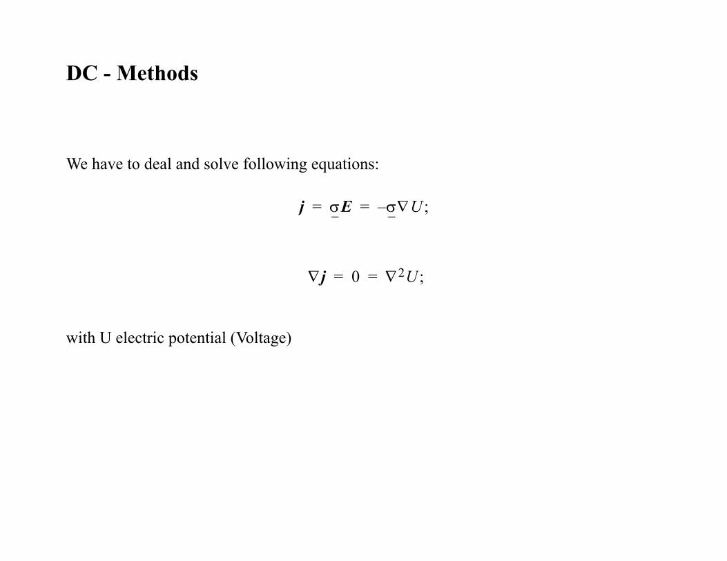
DC - Methods

We have to deal and solve following equations:

;

;

with U electric potential (Voltage)

j σE σ∇U–= =

∇j 0 ∇2U= =

Ohm’s Law:

U Voltage, I current, R resistivity

Rewriting the equation leads to:

specific resistivity

ratio length to cross section of conductor

Rewriting current density law:

;

i.e. the tensor of specific resistivity is reciprocal to the tensor of conductivity

U RI=

U ρ lq---I=

ρlq---

j 1ρ---E=

Assumption (often made): isotropic subsurface structure

; scalar

Question: Which quantities we are able to measure?

current and voltage differences!

j 1ρ---E 1

ρ---∇U= = ρ

Buried source in homogeneous full space:

Exercise: How doe the current lines look like if we assume a homogenous half space?Hint: free surface conditions can be modelled by a mirror charge placed in the same dis-tance in open space

Q

equipotential lines

lines of current (j)

(U=const)

Solving Laplace equation:

;

(problem is radial symmetric);

multiplying with and integrating the equation:

.

repeated integration gives the solution:

.

What about A & B? when

We can only measure current (not the density) directly. Therefore we must integrate over the surface of the complete equipotential shell in a distance of r:

.

∇2U d2Udr2---------- 2

r---⎝ ⎠⎛ ⎞ dV

dr-------+ 0= =

r2

dVdr------- A

r2----=

V Ar---– B+=

V 0→ r ∞→ B⇒ 0=

I 4πr2j=

The equation for the current is then:

Now we can estimate the constant A as:

Substitution gives desired equation for specific resistivity:

.

In case of half space and electrode at the surface we have to divide the latter equation by a factor of 2:

;

I 4πr2j σ4πr2– dUdr------- 4πσA–= = =

A Iρ–4π--------=

ρ 4πrUI

--------------=

ρ 2πrUI

--------------=

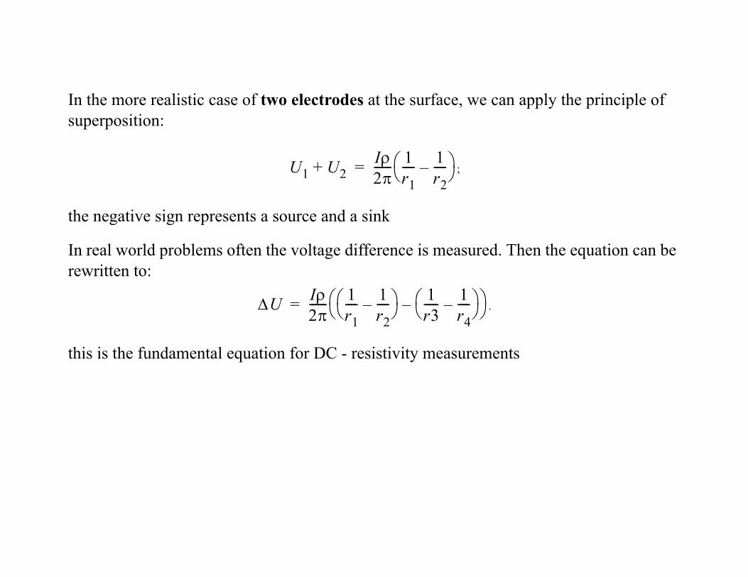
In the more realistic case of two electrodes at the surface, we can apply the principle of superposition:

;

the negative sign represents a source and a sink

In real world problems often the voltage difference is measured. Then the equation can be rewritten to:

.

this is the fundamental equation for DC - resistivity measurements

U1 U2+ Iρ2π------ 1

r1---- 1

r2----–⎝ ⎠

⎛ ⎞=

∆U Iρ2π------ 1

r1---- 1

r2----–⎝ ⎠

⎛ ⎞ 1r3----- 1

r4----–⎝ ⎠

⎛ ⎞–⎝ ⎠⎛ ⎞=

Using specific electrode configuration the latter equation can be much more simplified (Schlumberger, Wenner, Dipol-Dipol etc.):

with geometry factor (depending on the configuration used)

I

C1 C2UP2P1

r1 r2

r3 r4

ρs k∆UI--------=

k

2) Known Problems:

a) Anisotropy:

Microanisotropiefactor is defined as:

;

transversal resistivity;

longitudinal resistivity

Mean value of resistivity is defined as: .

Effect of micro anisotropy wrong layer thickness!

θρtρl----

σlσt----- 1>= =

ρtρl

ρ ρtρl=⇒

.

Anisotropy is one of the main sources of errors in DC-resistivity measurements! With-out a prior knowledge no distinction possible!

ρt

ρl

H ρs ρ=θH

b) Non-uniqueness Problem

Same data can be modelled equally well with different model parameters

.

c) Thin layers

thin layers in greater depth are often missed. In order to judge whether this happens we can define a “relative thickness” measure:

layer thickness; depth of layer.

To recognize a layer the following relation must be fulfilled:

d) Topography/surface conditions/3D effects

• resistivity measurements are strongly influenced by surface conditions (weathering; water content etc.)

• topography has a similar effect; valleys - current is focussed; ridges - current is dis-persed. Important for slopes

• strong variations of apparent resistivity for short electrode spacings indicate surface/topography problems

Hh---- m=

H h

m 1>

10°>

• 3D bodies can show up with wrong parameters when modelled by 2D or even 1D mod-els:

3) Common electrode configurations and sensitivity

Choosing the best configuration for your problem:

• sensitivity in vertical and horizontal direction

• desired penetration depth

• horizontal data coverage

• signal strength

i) Wenner • sensitive for changes in vertical - insensitive for changes in horizontal direction• high signal strength• depth resolution is in between other configurations;

ii) Schlumberger (-Wenner)• increased horizontal resolution (ref. Wenner)• increased vertical resolution (10% ref. Wenner)• decreased signal strength• increased data coverage

iii) Dipol-Dipol• widely used configuration (minor EM coupling)• high horizontal sensitivity; low vertical sensitivity• low depth resolution;• low signal strength;• best method to map lateral structures

.

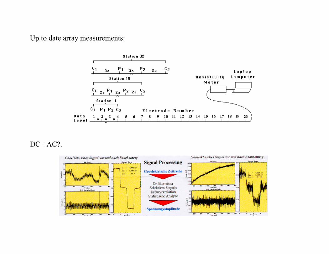
Up to date array measurements:

DC - AC?.

4) Measurement and Interpretation

• 1D experiment ~ 10 - 20 measurements/profile• 2D experiment ~ 100-1000 measurements/profile

costs!

a) 1D Sounding

• computing the apparent specific resistivity vs. the half profile length on a double loga-rithmic scale;

• in order to estimate the number of layers and layer parameters you can choose between different possibilities:

i) computing sounding curves with predefined simple models using sim-ple software (2-4 layers)

ii) computing the optimal model graph by comparing with master graphsiii) estimating the optimum model graph with starting models from i) &

ii)

⇒

Aufgabe 2: Bestimmen Sie die scheinbaren spezifischen Widerstände aus folgender Wid-erstandssondierung; Tragen Sie dies auf doppellogarithmischen Papier auf ( gegen ). Was kann über die Anzahl der Schichten und deren relatives Widerstandsverhältnis ausge-sagt werden? Bestimmen Sie die Schichtmächtigkeit und den scheinbaren spezifischen Widerstand der ersten Schicht.

ρsl2---

b) 2D Sounding

• Variations possible in vertical and horizontal direction closer to reality; all varia-tion perpendicular to the profile are neglected

• good compromise between model error and experiment costs.

• DC-array measurements (>25 electrodes); results plotted as pseudo-section.

⇒

NOTE: Pseudo-sections are not the result of the measurement but rather a first step in interpretation and data quality check. In order to get the “true” resistivity of the subsur-face, we have to invert (!?) the data using computer software.

ALSO NOTE: non-uniqueness of DC-measurements.

Aufgabe: Erstellen Sie eine Pseudosektion aus folgenden Messdaten. Was lässt sich über den Untergrund aussagen?

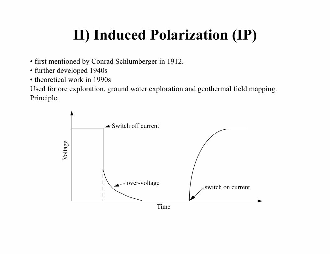
II) Induced Polarization (IP)• first mentioned by Conrad Schlumberger in 1912.• further developed 1940s• theoretical work in 1990sUsed for ore exploration, ground water exploration and geothermal field mapping.Principle.

Switch off current

over-voltage

Volta

ge

Time

switch on current

1) Basics• physical reasons only partially known. • two mechanisms are known better:

a) Electrode Polarization (Grain Polarization)

• Nernst Potential caused by local concentration differences of solution:

;

R universal gas constant; T temperature in Kelvin; n valence; F Faraday’s constant; solution concentrations.

UNRTnF-------

C1C2-------⎝ ⎠⎛ ⎞ln=

C1 2,

• Zeta-potential; adsorption of anions at veins and fissures of quartz or pegmatite - impor-tant for clay bodies

b) Electrolytic Polarization

.

2) Measurement of IP-Effect

• most commonly Dipol-Dipol configuration used

• measurement electrodes must be un-polarized electrodes

a) Time domain measurements

Definition of Chargeability:

Definition of apparent Chargeability:

UpU------ M=

Ma1U0------ Up t( ) td

t1

t2

∫AU0------= =

b) Frequency domainPercentage frequency effect:

mit ;

.

Metal Factor: ; with ;

PFEρs f1( ) ρs f2( )–( )

ρ f1( )----------------------------------------100= ρs f1( ) ρs f2( )>

MF PFEρs

-----------10i= i 2…5=

3) Interpretation • commonly the data or parameters (PFE,MF etc.) are plotted in pseudo sections.

This is NOT the result of true subsurface structure! Inversion⇒