iac-09.d1.6.1 comparative reliability of geo, …...1 iac-09.d1.6.1 comparative reliability of geo,...
TRANSCRIPT

1
IAC-09.D1.6.1
COMPARATIVE RELIABILITY OF GEO, LEO, AND MEO SATELLITES
Thomas Hiriart Graduate Research Assistant, Georgia Institute of Technology, Atlanta, USA
Jean-Francois Castet Graduate Research Assistant, Georgia Institute of Technology, Atlanta, USA
Jarret M. Lafleur Graduate Research Assistant, Georgia Institute of Technology, Atlanta, USA
Joseph H. Saleh Assistant Professor, Georgia Institute Technology, Atlanta, USA
ABSTRACT
Reliability has long been a major consideration in the design of space systems, and in recent years it has become an essential metric in spacecraft design trade-space exploration and optimization. The purpose of this paper is to statistically derive and compare reliability results of Earth-orbiting satellites as a function of orbit type, namely geosynchronous orbits (GEO), low Earth orbits (LEO) and medium Earth orbits (MEO). Using an extensive database of satellite launches and failures/anomalies, life data analyses are conducted over three samples of satellites within each orbit type and successfully launched between 1990 and 2008. Because the dataset is censored, the Kaplan-Meier estimator is used to estimate the reliability functions. Plots of satellite reliability as a function of orbit altitude are provided for each orbit type, as well as confidence bounds on these estimates. Using analytical techniques such as maximum likelihood estimation (MLE), parametric fits are conducted on the previous nonparametric reliability results using single Weibull and mixture distributions. Based on these parametric fits, a comparative reliability analysis is provided identifying similarities and differences in the reliability behaviors of satellites in these three types of orbits. Finally, beyond the statistical analysis, this work concludes with several hypotheses for structural/causal explanations of these trends and difference in on-orbit failure behavior.
1. INTRODUCTION
Reliability has long been recognized as a critical attribute for space systems, and potential causes of on-orbit failures are carefully sought for identification and elimination through careful design and part selection, and extensive testing prior to launch. Unfortunately, despite the recognition of its importance, limited on-orbit failure data and statistical analyses of satellite reliability exist in the technical literature. To help fill this gap, Castet and Saleh (2009) recently collected failure data for 1,584 Earth-orbiting satellites successfully launched between January 1990 and October 2008 [1]. The authors conducted a nonparametric analysis of satellite reliability and provided empirical curves of satellite reliability with 95% confidence
intervals, as presented in Fig. 1. One limitation the authors recognized and discussed in [1] is the lumping together of all Earth-orbiting satellites into one category, and statistically analyzing their “collective” failure behavior. It can be argued that no two (or more) satellites are truly alike, and that every satellite operates in a distinct environment. As a result, the situation of the space industry is very different from that for example of the semi-conductor industry where data on, say, millions of identical transistors operating under identical environmental conditions are available for statistical analysis. The consequence is that in the absence of “satellite mass production,” statistical analysis of satellite failure and reliability data faces the dilemma of choosing between calculating precise “average” satellite reliability on the one hand, or

2
deriving a possibly uncertain “specific” satellite reliability on the other hand.
0.87
0.88
0.89
0.90
0.91
0.92
0.93
0.94
0.95
0.96
0.97
0.98
0.99
1.00
0 1 2 3 4 5 6 7 8 9 10 11 12 13 14 15Time after successful orbit insertion (years)
Rel
iab
ility
Nonparametric estimation
95% confidence interval -upper bound95% confidence interval -lower bound
Figure 1: Satellite reliability with 95%
confidence intervals [1] This dilemma is explained in the following two possible approaches. The first approach is to lump together different satellites and analyze their “collective” on-orbit failure behavior (assuming that the failure times of the satellites are independent and identically distributed (iid)). The advantage of doing so is that one can work with a relatively large sample and thus obtain some precision and a narrow confidence interval for the “collective” reliability analyzed. The disadvantage is that the iid assumption may not be realistic, and the “collective” reliability calculated (with precision) may not reflect the specific reliability of a particular type of spacecraft. The second approach is to specialize the data, for example for specific spacecraft platform or mission type, or for satellites in particular orbits. The advantage of doing so is that the reliability analyzed is specific to the type of spacecraft considered (it is no longer a “collective” on-orbit reliability). The disadvantage is that the sample size is reduced, and as a consequence, the confidence interval expands (i.e., the results become increasingly uncertain). Given the available number of satellites (a few thousands), data specialization, which could reduce the sample size to say fewer than a hundred data points, would result in significantly large confidence intervals, and thus highly dispersed and uncertain “specific” satellite reliability calculations.
In this paper, we adopt the second approach. We discuss this approach in [2] and [3] and analyze on-orbit reliability of satellites by mission type,
and mass categories (data for specific satellite platforms and by manufacturer is also available). Reliability of satellite subsystems can be found in [4]. From a statistical perspective, several parameters (covariates) or characteristics of the design can affect the probability of failure of satellites. For example, the spacecraft complexity, its orbit, the number of instruments on-board or its payload size, to name a few, have some implications on satellite reliability. One factor impacting satellite reliability might be the orbit type since the choice of orbit can impact design choices on board the spacecraft as well as the system’s operating environment. Several questions follow this observation: for example, are different spacecraft orbits correlated with different failure behaviors on-orbit? Do low Earth orbit (LEO) satellites for example exhibit different failure behaviors than geosynchronous orbit (GEO) satellites? Do satellites in different orbits exhibit varying degrees of infant mortality? Etc. In this paper, we conduct statistical analysis of satellite reliability with orbit as a covariate. Our analysis is based on a data set of 1,488 Earth-orbiting satellites successfully launched between January 1990 and October 2008. We first categorize these satellites by orbit: geosynchronous orbit (GEO), low Earth orbit (LEO) and medium Earth orbit (MEO). We then conduct nonparametric analysis of satellite reliability for each orbit category using the Kaplan-Meier estimator. Using analytical techniques such as Maximum Likelihood Estimation (MLE) and least squares regression, we then conduct parametric analysis assuming 1- and 2-Weibull mixture distributions. Based on these parametric fits, we provide a comparative reliability analysis identifying similarities and differences in the reliability behaviors of satellites in these three types of orbits. Finally, beyond the statistical analysis, we conclude this work with several hypotheses for structural/causal explanations of these trends and difference in on-orbit failure behavior.
2. DATABASE AND DATA DESCRIPTION
For the purpose of this study, we used the SpaceTrak® database [5]. This database provides a history of on-orbit satellite failures and anomalies, as well as launch histories since 1957 and is considered one of the most
3
authoritative in the space industry with data for over 6,400 spacecraft. The sample we analyzed consists of 1,488 satellites. We restricted the present study to Earth-orbiting satellites successfully launched between January 1990 and October 2008. In order to compute the reliability, we used what is referred to in the database as a Class I failure, that is, a retirement of a satellite due to failure. For each spacecraft in our sample, we collect: 1) its orbit type; 2) its launch date; 3) its failure date, if failure occurred; and 4) the “censored time,” if no failure occurred. This last point is further explained in the following
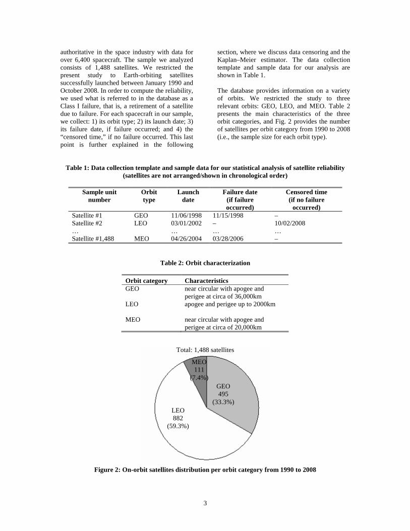
section, where we discuss data censoring and the Kaplan–Meier estimator. The data collection template and sample data for our analysis are shown in Table 1. The database provides information on a variety of orbits. We restricted the study to three relevant orbits: GEO, LEO, and MEO. Table 2 presents the main characteristics of the three orbit categories, and Fig. 2 provides the number of satellites per orbit category from 1990 to 2008 (i.e., the sample size for each orbit type).
Table 1: Data collection template and sample data for our statistical analysis of satellite reliability (satellites are not arranged/shown in chronological order)
Sample unit
number Orbit type
Launch date
Failure date (if failure occurred)
Censored time (if no failure
occurred) Satellite #1 GEO 11/06/1998 11/15/1998 – Satellite #2 LEO 03/01/2002 – 10/02/2008 … … … … Satellite #1,488 MEO 04/26/2004 03/28/2006 –
Table 2: Orbit characterization
Orbit category Characteristics GEO near circular with apogee and
perigee at circa of 36,000km LEO apogee and perigee up to 2000km
MEO near circular with apogee and
perigee at circa of 20,000km
Figure 2: On-orbit satellites distribution per orbit category from 1990 to 2008
Total: 1,488 satellites
MEO 111
(7.4%) GEO 495
(33.3%) LEO 882
(59.3%)
4
3. NON-PARAMETRIC SATELLITE RELIABILITY ANALYSIS
In this section, we briefly review censoring in statistical data analysis and the Kaplan-Meier estimator of reliability when the underlying data is right-censored, as is the case in our sample. Nonparametric means that the statistical analysis does not assume any specific parametric distribution (also referred to sometimes as distribution-free analysis). We then provide the reliability results for satellites in GEO, LEO, and MEO. Censored Data Sample and Kaplan-Meier estimator
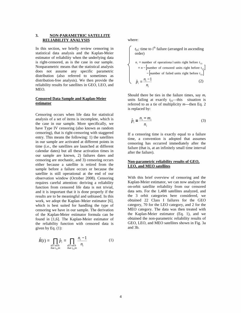
Censoring occurs when life data for statistical analysis of a set of items is incomplete, which is the case in our sample. More specifically, we have Type IV censoring (also known as random censoring), that is right-censoring with staggered entry. This means the following: 1) the satellites in our sample are activated at different points in time (i.e., the satellites are launched at different calendar dates) but all these activation times in our sample are known, 2) failures dates and censoring are stochastic, and 3) censoring occurs either because a satellite is retired from the sample before a failure occurs or because the satellite is still operational at the end of our observation window (October 2008). Censoring requires careful attention: deriving a reliability function from censored life data is not trivial, and it is important that it is done properly if the results are to be meaningful and unbiased. In this work, we adopt the Kaplan–Meier estimator [6], which is best suited for handling the type of censoring we have in our sample. The derivation of the Kaplan-Meier estimator formula can be found in [1,6]. The Kaplan-Meier estimator of the reliability function with censored data is given by Eq. (1):
∏∏≤≤
−==tthat t
such alltthat t
such all(i)(i)
1ˆ)(ˆ
i i
i
ii n
nptR (1)
where:
t(i): time to ith failure (arranged in ascending order)
[ ][ ](i)
(i)
(i)
tbeforeright units failed ofnumber
tbeforeright units censored ofnumber
tbeforeright units loperationa ofnumber
−
−=
=
n
ni
i
ii n
np
1ˆ
−= (2)
Should there be ties in the failure times, say mi units failing at exactly t(i)—this situation is referred to as a tie of multiplicity m—then Eq. 2 is replaced by:
ˆ p i ==== ni −−−− mi
ni
(3)
If a censoring time is exactly equal to a failure time, a convention is adopted that assumes censoring has occurred immediately after the failure (that is, at an infinitely small time interval after the failure). Non-parametric reliability results of GEO, LEO, and MEO satellites
With this brief overview of censoring and the Kaplan-Meier estimator, we can now analyze the on-orbit satellite reliability from our censored data sets. For the 1,488 satellites analyzed, and the 3 orbit categories here considered, we obtained 22 Class I failures for the GEO category, 70 for the LEO category, and 2 for the MEO category. The data was then treated with the Kaplan-Meier estimator (Eq. 1), and we obtained the non-parametric reliability results of GEO, LEO, and MEO satellites shown in Fig. 3a and 3b.

5
Figure 3a: Nonparametric results of GEO and LEO satellites reliability
Figure 3b: Nonparametric result of MEO satellites reliability
6
Figure 3a and 3b are known as the Kaplan plots of reliability. Vertical cuts across Fig. 3 read as follows, for example:
• The most likely estimate of GEO satellites reliability at t = 1 year on-orbit
is R = 98.7%.
• The most likely estimate of GEO satellites reliability at t = 7 year on-orbit
is R = 96.8%. The Kaplan plots for the GEO, LEO, and MEO satellites allow us to visually identify some important trends in satellite reliability and on-orbit failure behavior. For example:
1. GEO satellites exhibit a small infant mortality, with a reliability dropping to approximately 98.7% after one year. In addition, GEO satellites exhibit a clear wear-out failure behavior between 6 and 12 years, with a reliability dropping from 97.5% to 92.5% (Fig. 3a).
2. LEO satellites exhibit a significant infant mortality, with a reliability dropping to 97% after one year. In addition, between the third and the sixth year, a “light” wear-out failure behavior can be observed with a reliability dropping from approximately 96.5% to 95% (Fig. 3a).
3. For the MEO satellites (Fig. 3b), only two
failures can be observed over 111 MEO satellites. As a result, no significant conclusions can be drawn about the nonparametric reliability results of these satellites.
These trends will be explored more closely and analytically in Sections 4 and 5.
4. PARAMETRIC RELIABILITY ANALYSIS
Nonparametric analysis provides important results since the reliability calculation is not constrained to fit any particular pre-defined lifetime distribution. However, this flexibility makes nonparametric results neither easy nor convenient to use for various purposes often encountered in engineering design (e.g., reliability-based design optimization). In addition, some failure trends and patterns are
more clearly identified and recognizable with parametric analysis. Several possible methods are available to fit a parametric distribution to the nonparametric reliability function (as provided by the Kaplan-Meier estimator). In the following, we present two parametric methods based on the Weibull distribution to fit the nonparametric reliability of satellites in each orbit category discussed previously. Weibull distribution
The Weibull distribution is one of the most commonly used distribution in reliability analysis. Its reliability (or survivor) function can be written as follows:
−=β
θt
tR exp)( for t ≥ 0 (4)
where β is the shape parameter (dimensionless) and θ the scale parameter (units of time), both nonnegative. The reason for the wide adoption of the Weibull distribution is that it is quite flexible, and with an appropriate choice of the shape parameter β, it can capture different kinds of failure behaviors. For example, when 0 < β < 1, the Weibull distribution models infant mortality (which corresponds to a decreasing failure rate); when β = 1, the Weibull distribution becomes equivalent to the Exponential distribution (constant failure rate); and when β > 1, the Weibull distribution models wear-out failures (which corresponds to an increasing failure rate). In previous publications, we demonstrated the appropriateness of the Weibull distribution as a parametric model for satellite reliability [1,4,7]. In this work, we first derive Weibull fits for the three nonparametric reliability results using the Maximum Likelihood (MLE) procedure. However, the parametric results will be shown to be within 0.6 to 3.2 percentage points of the “benchmark” nonparametric results, and for our purposes, these results are not sufficiently accurate. We therefore proceed with deriving mixture Weibull distributions for the nonparametric results and demonstrate a significant improvement in the accuracy of the parametric fits. The details are discussed next.

7
Maximum Likelihood Estimation (MLE) of single Weibull fit
Details of the Maximum Likelihood Estimation procedure can be found in [8], and its analytic derivation is provided in [4]. When applied to the nonparametric reliability results shown in Fig. 3a and 3b, the MLE procedure yields the Weibull parameter estimates for each satellite orbit category. The results are provided in Table 3.
Table 3: Maximum Likelihood Estimates of the Weibull parameters for satellite reliability
across the three orbit categories
Orbit category β θ years GEO 0.7190 582.5 LEO 0.3473 34048.9 MEO 1.6347 79.4
The information in Table 3 reads as follows. Consider for example the GEO satellites. Its nonparametric reliability is best approximated by the following MLE-derived Weibull distribution:
−=719.0
5.582exp)(
ttRGEO
(5)
The values of the shape parameter (β = 0.7190) and the scale parameter (θ = 582.5) are the Maximum Likelihood Estimates. Figure 4 shows the nonparametric reliability curve and the MLE-
derived Weibull fit for the three orbit categories. For satellites in LEO, Fig. 4 provides a visual verification that the MLE-derived Weibull distribution is a satisfying fit for the nonparametric reliability. It is difficult to derive the same conclusion for the two other orbit categories. The goodness-of-fit of the Weibull distribution is reflected in this work by the maximum and average errors over 15 years between the nonparametric reliability results (the “benchmark” results) and the Weibull fit. Table 4 provides the maximum and average error between the nonparametric reliability and the Weibull fit for the three orbit categories. Despite this reasonable accuracy of the parametric fit, Fig. 4 shows that the single Weibull distribution does not fully capture the failure trends in the data, especially for the GEO and MEO satellites. To improve the quality of the parametric fit, we derive in the next subsection mixture Weibull distributions for the non-parametric reliability results derived in Section 3.
Table 4: Error between the nonparametric reliability and MLE Weibull fit for each
satellite category
Orbit category
Maximum error
(percentage point)
Average error
(percentage point)
GEO 1.6 0.7 LEO 0.6 0.2 MEO 3.2 1.0
GEO category LEO category MEO category
Figure 4: Nonparametric reliability and single Weibull fit

8
Mixture distributions
Several distributions such as the Exponential, Weibull, or Lognormal, can be used as a basis for linear combination to generate a mixture distribution. In this subsection, we maintain the Weibull as the basis for our parametric calculations and derive mixture of two Weibull distributions for the nonparametric satellite reliability of each orbit category. The parametric reliability model with a mixture of two Weibull distributions can be expressed as follows:
−−+
−=
21
21
exp)1(exp)(ββ
θα
θα tt
tR (6)
The parameter α is used to modify the relative weight given to each Weibull distribution in the mixture. A generalized expression for n mixture distributions is provided in [9]. We restrict our calculations in this work to n = 2 since as will be shown shortly, the results are significantly accurate and the 2-Weibull distributions follows with notable precision the different failure trends in the nonparametric results. Limited incremental accuracy is provided by 3-Weibull mixture distributions. Increasing n provides insignificant accuracy improvement.
The nonlinear least squares method provides us with the best fits for the parameters of the 2-Weibull mixture distribution for each orbit category. The results are provided in Table 5. For the three orbit categories, the new parametric fit of the reliability using a 2-Weibull mixture distribution accurately follows the nonparametric reliability, as shown in Fig. 5. It is worth pointing out that the first Weibull element with a shape parameter β1 < 1 captures satellite infant mortality while the second Weibull element with a shape parameter β2 > 1 captures satellite wear-out failures. As expected, the fits provided by the mixture distributions approach for the three orbits categories are better than those provided by the MLE approach. Table 6 provides the 2R coefficients and the sum of the squares of errors (SSE) of the three mixture distributions formulated for each orbit category. The 2R coefficients of the fits are higher than 97% for the three categories. To gauge the precision improvement between the single Weibull and the 2-Weibull mixture distributions, we calculate both the maximum and the average error between the nonparametric reliability (the benchmark results) and the parametric models. The results are shown in Table 7.
Table 5: 2-Weibull mixture distribution parameters
Orbit category α β1 β2 θ1 θ2 years
GEO 0.0496 4.1070 0.3300 9.8 661600.0 LEO 0.9927 0.2997 68.6300 136100.0 14.4 MEO 0.9526 1.4790 8.3600 101900.0 6.0
GEO category LEO category MEO category
Figure 5: Nonparametric reliability and 2-Weibull mixture fit for the three satellite categories

9
Table 6: Goodness-of-fit of the 2-Weibull mixture distribution for each satellite category
Ceofficient Orbit category GEO LEO MEO 2R 0.9908 0.9845 0.9749
SSE 0.03978 0.01698 0.08776
Table 7: Error between the nonparametric reliability and the parametric models over 15 years
Orbit category Error Parametric fit
percentage point Single Weibull 2-Weibull mixture
maximum error 1.6 0.7 GEO
average error 0.7 0.2
maximum error 0.6 0.4 LEO
average error 0.2 0.1
maximum error 3.2 1.8 MEO
average error 1.0 0.2
As seen in Table 7, the 2–Weibull mixture distribution is significantly more accurate than the single Weibull distribution in capturing the (benchmark) nonparametric satellite reliability. Section 3 briefly presented the general trends in the nonparametric reliability curves of each orbit category. In order to lead further investigations on the behavioral differences between the three satellite categories, the next section provides a detailed comparative analysis of the satellite reliability across orbit categories based on the mixture distributions previously developed.
5. COMPARATIVE ANALYSIS OF SATELLITE RELIABILITY ACROSS ORBIT CATEGORIES
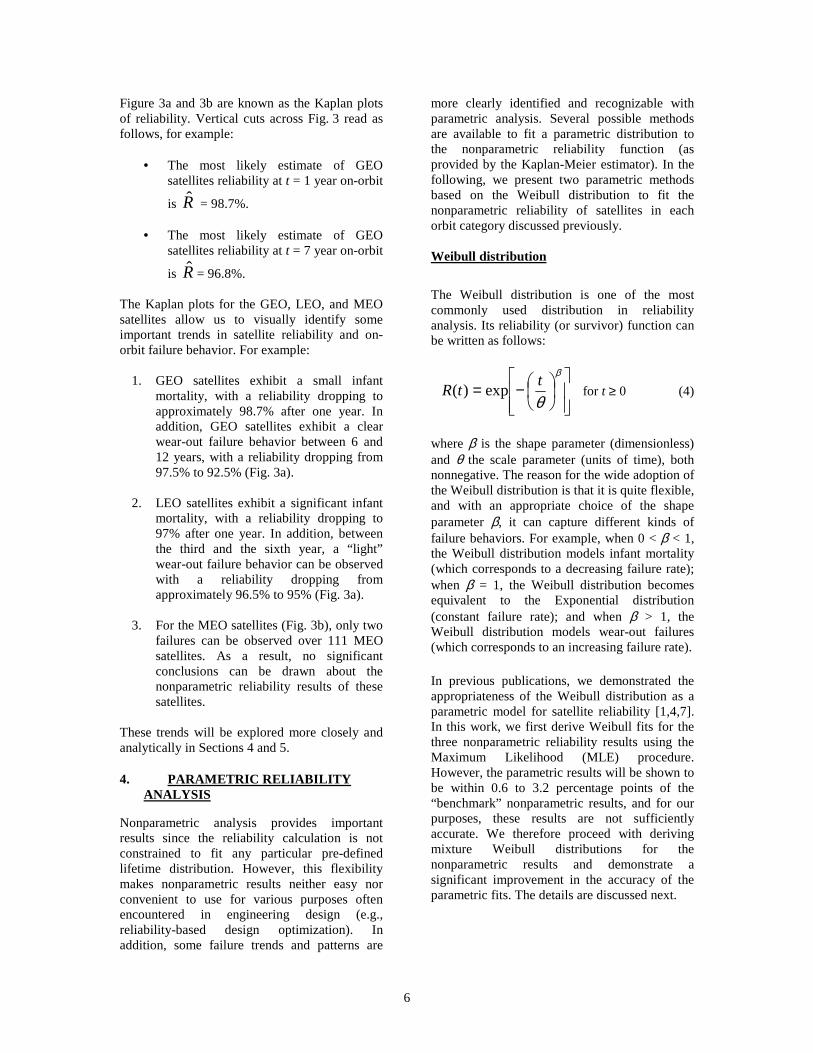
This section identifies periods of time during which the reliability of the orbit categories show similarities or differences in their behavior. Figure 6 presents the absolute difference in satellite reliability for each pair of orbit categories: LEO/MEO, LEO/GEO, and MEO/GEO. More than characterizing the amplitude of the difference itself, we ultimately
seek to identify a period of time during which the difference remains approximately constant, meaning that the two reliability curves have the same behavior. For example, a significant increase of the absolute difference early in time after successful orbit insertion during ],0[ 1t ,
followed by a relatively constant evolution of the difference during ],[ 21 tt , would mean that the
two reliability curves do not exhibit similar infant mortality behavior during ],0[ 1t but also
that they do show similar behavior later in time during ],[ 21 tt . First we can notice that all the
three differences jump up to 1 percentage point during the first year following orbit insertion. This result indicates that satellites across the three orbit categories have different failure behavior early on orbit, that is they have different infant mortality behavior. A quick glance at Fig. 6 also reveals that significant periods of time during which any of the three reliability differences remains roughly constant are difficult to find. The only period of interest would eventually be between 3 and 6 years for
10
the LEO/GEO difference but yet, the periods responsible for similarities and differences between reliability profiles are not explicitly identified on a plot like Fig. 6.
0 1 2 3 4 5 6 7 8 9 10 11 12 13 14 150
1
2
3
4
5
Time after successful orbit insertion (years)
Ab
solu
te d
iffer
ence
bet
wee
n r
elia
bili
ty c
urv
es(p
erce
nta
ge
po
ints
)
LEO - MEOLEO - GEOMEO - GEO
Figure 6: Pairwise differences in satellite reliability over time
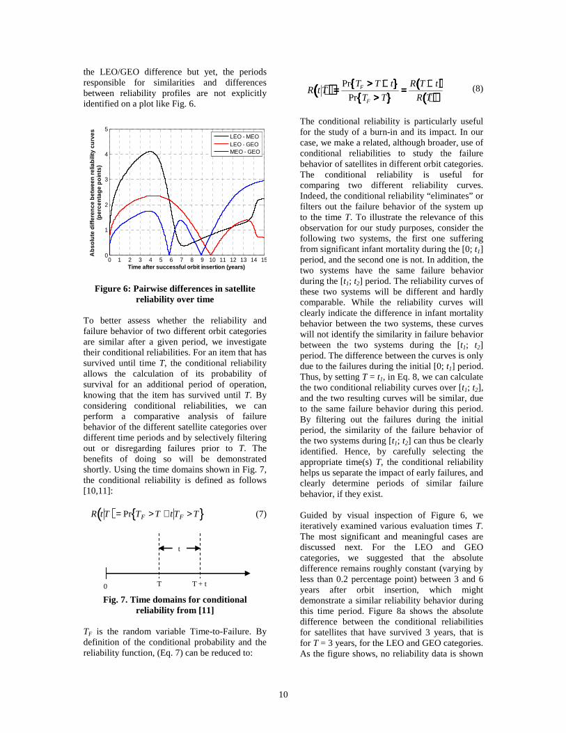
To better assess whether the reliability and failure behavior of two different orbit categories are similar after a given period, we investigate their conditional reliabilities. For an item that has survived until time T, the conditional reliability allows the calculation of its probability of survival for an additional period of operation, knowing that the item has survived until T. By considering conditional reliabilities, we can perform a comparative analysis of failure behavior of the different satellite categories over different time periods and by selectively filtering out or disregarding failures prior to T. The benefits of doing so will be demonstrated shortly. Using the time domains shown in Fig. 7, the conditional reliability is defined as follows [10,11]:
R t T( )= Pr TF > T + t TF > T{ } (7)
0 T T + t
t
Fig. 7. Time domains for conditional
reliability from [11]
TF is the random variable Time-to-Failure. By definition of the conditional probability and the reliability function, (Eq. 7) can be reduced to:
R t T(((( ))))====Pr TF >>>> T ++++ t{{{{ }}}}
Pr TF >>>> T{{{{ }}}}====
R T ++++ t(((( ))))R T(((( ))))
(8)
The conditional reliability is particularly useful for the study of a burn-in and its impact. In our case, we make a related, although broader, use of conditional reliabilities to study the failure behavior of satellites in different orbit categories. The conditional reliability is useful for comparing two different reliability curves. Indeed, the conditional reliability “eliminates” or filters out the failure behavior of the system up to the time T. To illustrate the relevance of this observation for our study purposes, consider the following two systems, the first one suffering from significant infant mortality during the [0; t1] period, and the second one is not. In addition, the two systems have the same failure behavior during the [t1; t2] period. The reliability curves of these two systems will be different and hardly comparable. While the reliability curves will clearly indicate the difference in infant mortality behavior between the two systems, these curves will not identify the similarity in failure behavior between the two systems during the [t1; t2] period. The difference between the curves is only due to the failures during the initial [0; t1] period. Thus, by setting T = t1, in Eq. 8, we can calculate the two conditional reliability curves over [t1; t2], and the two resulting curves will be similar, due to the same failure behavior during this period. By filtering out the failures during the initial period, the similarity of the failure behavior of the two systems during [t1; t2] can thus be clearly identified. Hence, by carefully selecting the appropriate time(s) T, the conditional reliability helps us separate the impact of early failures, and clearly determine periods of similar failure behavior, if they exist. Guided by visual inspection of Figure 6, we iteratively examined various evaluation times T. The most significant and meaningful cases are discussed next. For the LEO and GEO categories, we suggested that the absolute difference remains roughly constant (varying by less than 0.2 percentage point) between 3 and 6 years after orbit insertion, which might demonstrate a similar reliability behavior during this time period. Figure 8a shows the absolute difference between the conditional reliabilities for satellites that have survived 3 years, that is for T = 3 years, for the LEO and GEO categories. As the figure shows, no reliability data is shown

11
until t = T. Until t = 6 years, the absolute difference between the conditional reliabilities varies very little and remains below 0.2 percentage points. After t = 6 years, the absolute difference between the conditional reliabilities increases significantly, suggesting a divergence of the two failure behaviors of satellites in LEO and GEO. This phenomenon can be verified in Fig. 8b, which shows the conditional reliabilities evaluated for T = 3 years for the GEO and LEO satellites. The two reliability curves are almost overlapping between 3 and 6 years, then a significant divergence occurs between the two curves after t = 6 years.
0 1 2 3 4 5 6 7 8 9 10 11 12 13 14 150.0
0.5
1.0
1.5
2.0
2.5
3.0
3.5
4.0
4.5
5.0
Time after successful orbit insertion (years)
Ab
solu
te d
iffe
ren
ce b
etw
een
co
nd
itio
nal
relia
bili
ties
at
T =
3 y
ears
(p
erce
nta
ge
po
ints
)
0 1 2 3 4 5 6 7 8 9 10 11 12 13 14 150.92
0.93
0.94
0.95
0.96
0.97
0.98
0.99
1.00
Time after successful orbit insertion (years)
Co
nd
itio
nal
rel
iab
iliti
es a
t T
= 3
yea
rs
LEOGEO
Regarding the other comparative reliability analyses, namely between LEO/MEO and GEO/MEO, no significant period of time was found showing similar failure behavior. In
addition, the small sample size of the MEO satellites (111 satellites) and only 2 failures renders it difficult to make strong inferences about the actual reliability and on-orbit failure behaviors of these satellites (more details on this point can be found in the appendix). In the next section, we discuss several hypotheses for possible structural/causal explanations of the difference in reliability and failure behavior of satellites across orbit categories.
6. HYPOTHESES FOR CAUSALITY ANALYSIS
The previous sections demonstrated that there are significant differences in the reliability and failure behavior of the LEO and GEO satellites. This section explores possible causes of these differences. The most obvious factor that varies from one orbit category to another is the space environment. The space operating environment strongly influences the performance and lifetime of on-orbit satellites and can lead to costly malfunctions or loss of subsystems and spacecraft [12]. The space environment, as a function of orbit choice, also impacts design decisions and has implications on satellite size, weight, complexity, and cost [13], all of which can impact satellite reliability. Programmatic considerations can also be important influencing factors of satellite reliability. These hypotheses are discussed next.
Environmental Factors
Upper Atmosphere
One obvious difference between LEO and the higher MEO and GEO orbits is the rarefied atmosphere present in LEO. This results in aerodynamic drag that must be counteracted for a satellite to remain in orbit for long periods of time. Orbit lifetime for typical satellites is on the order of a few months at 300 km altitude and a few years at 400 km altitude [14]. However, orbit lifetime estimates are subject to significant uncertainty because they are limited by the accuracy of drag and space weather models [15]. Two well-known examples of unintended re-entries due to inadequate drag predictions are the American Skylab and Soviet Salyut 7 space stations. Skylab was originally expected to remain in orbit ten years after the last crew
Figure 8a: Absolute difference in conditional reliability evaluated for T = 3 years between GEO and LEO satellites
Figure 8b: Conditional reliabilities evaluated for T = 3 years between GEO
and LEO satellites

12
departed in 1974, allowing for potential servicing by the Space Shuttle. However, Skylab became the victim of unexpectedly high solar activity and re-entered in 1979 [16]. Similarly, it was intended for Salyut 7 to remain in orbit 8-20 years after its 1986 decommissioning for potential retrieval by the Soviet Buran space shuttle. However, it re-entered in February 1991 due to unexpected solar activity which raised upper atmospheric density by factors of 4-5. Furthermore, a local peak in solar activity in late January 1991 prevented the impact location from being known more accurately than within a half-orbit until just three hours prior to impact [15, 17]. Since atmospheric drag effects and their associated uncertainties typically manifest themselves gradually, they are rarely the direct causes of satellite failures. However, they do affect decommissioning dates for LEO satellites and may exacerbate the effects of otherwise more minor failures. For example, upper atmosphere drag on LEO satellites may result in shorter windows during which an operations team can effectively recover the satellite from propulsion, attitude control, or communications failures before drag losses or drag-induced torquing effects become too large. In addition, the upper atmosphere is associated with chemically corrosive effects of highly reactive species such atomic oxygen. This form of oxygen, predominant from about 200 km to 600 km in altitude, can react with organic films, composite materials, and metallized surfaces, causing degradation on sensor performance [18]. Solar arrays and space mirrors are an example of subsystems that encounter a degradation problem caused by the impact of atomic oxygen in the LEO environment [12, 19]. Extensive erosion due to atomic oxygen is one failure mechanism in LEO that does not exist in the GEO and MEO orbits.
Plasma and Magnetic Field
Ionization of the space environment is highly dependent on altitude. At about 300 km, 1% of the atmosphere is ionized while this number increases to 100% ionization in the geosynchronous environment. These charged particles, forming the plasma environment, charge the surface of any spacecraft within it to high negative voltages. If the local electric field exceeds the breakdown field along the surface of the material, it can trigger an electrostatic arc and
electromagnetic interference (EMI) large enough to disrupt electronic components [20]. This has been attributed as a major failure mode for GEO satellites, particularly as they emerge from an eclipse period into a solar storm [21]. At low altitude, this charged phenomenon only appears in the high latitudes regions, where auroral electrons collide with the spacecraft. It is yet much more common for higher orbits, such as GEO.
Radiation
There are several types of radiation that may threaten Earth-orbiting spacecraft. Since these types of radiation impact satellites in distinct altitude ranges, they are also candidate explanations for differences in reliability behavior among LEO, MEO, and GEO satellites. • The Van Allen radiation belts consist of
electrons and ions with energies greater than 30 keV. They are distributed nonuniformly within the magnetosphere up to a distance of 7 Earth radii. It is usually acknowledged that space missions beyond low Earth orbit leave the protection of the geomagnetic field, and transit the Van Allen belts. Thus they face more threats caused by the Van Allen radiations. The region between two to three Earth radii lies between the two radiation belts and is sometimes referred to as the “safe zone” [22].
• Solar particle events (SPEs) occur in association with solar flares. They are rapid increases in the flux of energetic particles, from 1 MeV to above 1 GeV, and can last from several hours to several days. Ultimately, they can lead to degradation of solar arrays or electro-optical sensors [13]. Depending on their energy level, the SPEs penetrate the Earth magnetosphere at different altitudes. It is more likely that they will impact high altitude orbits, such as geosynchronous orbits, than low-Earth orbits.
Thermal and Power Cycling
In addition to space environment effects, another substantial difference among the three orbit categories is the degree of thermal and power cycling. In a one-day period, a 400 km LEO satellite orbits the Earth about sixteen times, while a GEO satellite orbits the Earth once. As a
13
result, the LEO satellite cycles between eclipse and sunlight periods at least sixteen times as often as the GEO satellite, subjecting the LEO satellite to substantially more thermal and power cycling. It is reasonable to consider that thermal expansion and contraction effects could cause component fatigue, particularly for delicate components. It is also plausible that power subsystem cycling, especially for the battery’s charge and discharge in and out of eclipse, could cause different failure modes for satellites in LEO and GEO. Cycling effects may be one contributor to the substantial infant mortality exhibited in the LEO satellite reliability data. Programmatic Effects
A final hypothesis for differences in the observed LEO and GEO satellite reliability behavior deals with the effect of programmatic decisions. Typically, GEO satellites are designed for use over a period of time on the order of a decade or more. In contrast, LEO satellite design lifetimes are generally shorter, often less than five years. The development of potentially more expensive and longer-lived GEO satellites is likely to include more investment in quality control testing, and more focus on reliability, part selection, and redundancy. The much lower infant mortality for GEO satellites may be attributable to this system development consideration.
7. SUMMARY
We derived in this work nonparametric and parametric reliability results for Earth-orbiting satellites as a function of orbit type, namely geosynchronous orbits (GEO), low Earth orbits (LEO) and medium Earth orbits (MEO). We used an extensive database of satellite launches and on-orbit failures and anomalies to derive, using the Kaplan-Meier estimator, nonparametric reliability results for each satellite category. Next, using the Maximum Likelihood Estimation (MLE) technique and least squares regression, we derived parametric fits of the results with single and 2-Weibull mixture distributions. The parametric fits using the mixture distributions proved to be significantly accurate in capturing the failure trends in the nonparametric results. Based on these parametric fits, we provided a comparative reliability analysis identifying similarities and differences in the reliability behaviors of satellites in these three types of
orbits. Finally, beyond the statistical analysis, we concluded this work with several hypotheses for structural/causal explanations of these trends and difference in on-orbit failure behavior.
APPENDIX
Confidence interval analysis
The Kaplan-Meier estimator (Eq. 1) provides a maximum likelihood estimate of reliability but does not inform us about the dispersion around ˆ R (ti) . This dispersion is captured by the
variance or standard deviation of the estimator, which is then used to derive the upper and lower bounds for a 95% confidence interval (that is, a 95% likelihood that the actual reliability will fall between the two calculated bounds, with the Kaplan-Meier analysis providing us with the most likely estimate). The variance of the estimator is provided by Greenwood’s formula (Eq. 9), and the 95% confidence interval is determined by Eq. 10.
vˆ a r R(ti)[[[[ ]]]] ≡≡≡≡ σ 2(ti) ==== ˆ R (ti)[[[[ ]]]]2⋅⋅⋅⋅
m j
n j (n j −−−− m j )j≤≤≤≤ i
∑∑∑∑ (9)
R95%(ti) ==== ˆ R (ti) ±±±± 1.96⋅⋅⋅⋅ σ(ti) (10) More details about these equations can be found in [23, 24, 25]. When Eqs. (9) and (10) are applied to the data within each category along with the Kaplan-Meier estimated satellite reliability R (ti) shown in Fig. 3, we obtain the 95% confidence interval curves. These results for each orbit category of satellites are shown in Fig. 9. It shows for example that the GEO Satellites reliability at t = 1 year will be between 97.7% and 99.7% with a 95% likelihood—these values constitute the lower and upper bounds of the 95% confidence interval at t = 1 year. Notice that the dispersion of R(ti) around ˆ R (ti) increases with time. This increase in dispersion can be seen in Fig. 9 by the growing gap between the Kaplan–Meier estimated reliability and the confidence interval curves. This phenomenon illustrates the increasing uncertainty or loss of accuracy of the statistical analysis of satellite reliability with time resulting from the decreasing sample size.

14
GEO category LEO category MEO category Figure 9: Satellite reliability with 95% confidence intervals for each orbit category
REFERENCES [1] Castet, J.-F., Saleh, J. H., Satellite
Reliability: Statistical Data Analysis and Modeling, Journal of Spacecraft and Rockets, Vol. 46, No. 5, Sept/Oct 2009.
[2] Castet, J-F., Saleh, J. H., Geosynchronous
Communication Satellite Reliability: Statistical Data Analysis and Modeling, 27th AIAA International Communications Satellite Systems Conference (ICSSC 2009), Edinburgh, Scotland, 1-4 June 2009.
[3] Dubos, G. F., Castet, J-F., Saleh, J. H.,
Statistical Analysis of Satellite Reliability Specialized by Mass Categories: Does (Spacecraft) Size Matter?, 60th International Astronautical Congress, Daejeon, Republic of Korea, 12-16 October 2009.
[4] Castet, J-F., Saleh, J. H., Satellite and
Satellite Subsystems Reliability: Statistical Data Analysis and Modeling, Reliability Engineering and System Safety, Vol. 94, No. 11, pp. 1718-1728, Nov. 2009.
[5] Ascend SpaceTrak® database [online
database],URL:http://www.ascendworldwide.com/spacetrak.aspx.
[6] Kaplan, E. L., Meier, P., Nonparametric
Estimation from Incomplete Observations, Journal of the American Statistical Association 1958; 53(282): 457-481.
[7] Castet, J-F., Saleh, J. H., Modeling for
Nonparametric Satellite Reliability: Graphical Versus Maximum Likelihood Estimations, submitted to Journal of Spacecraft and Rockets, April 2009.
[8] Lawless, J. F., Statistical models and
methods for lifetime data, 2nd ed., New York: John Wiley & Sons, 2003.
[9] Castet, J-F., Saleh, J. H., Single versus
mixture Weibull distributions for nonparametric satellite reliability, submitted to Reliability Engineering and System Safety, May 2009.
[10] Ebeling, C. E., An Introduction to
Reliability and Maintainability Engineering, New York: McGraw-Hill, 1996.
[11] Kececioglu, D., Reliability Engineering
Handbook, Englewood Cliffs, N.J. : Prentice-Hall, 1991.
[12] Hastings, D., Garrett, H., Spacecraft-
Environment Interactions, New York: Cambridge University Press, 1996.
[13] Tribble, A. C., The Space Environment and
Survivability, in: Wertz, J. R., Larson, W. J., Space Mission Analysis and Design, Space Technology Library, 1999.
[14] Larson, W.J., and Wertz, J.R. (ed.), Space
Mission Analysis and Design, 3rd ed., Microcosm Press and Kluwer Academic Publishers, El Segundo, 1999.
[15] Doornbos, E. and Klinkrad, H., Modelling
of space weather effects on satellite drag, Advances in Space Research, Vol. 37, No. 6, 2006. pp. 1229-1239.
[16] Klinkrad, H. and Fritsche, B., Assessment
and Management of On-Ground Risk during Re-Entries, Joint ESA-NASA Space-Flight

15
Safety Conference, ESA SP-486, 2002. pp. 325-332.
[17] Lobachev, V., Pochukaev, V., Ivanov, N., et.
al., Navigation Support for the Salyut-7/Kosmos-1686 Orbiting Complex near Re-entry, ESA Journal, Vol. 16, No. 2, 1992. pp. 209-216.
[18] Visentine, J.T., Atomic Oxygen Effects
Measurements for Shuttle Missions STS-8 and 41-G, vols. I-III. NASA TM-100549, 1988.
[19]Mileti, S., Coluzzi, P., Marchetti, M.,
Degradation of silicon carbide reflective surfaces in the LEO environment, AIP Conference Proceedings, v 1087, p 67-74, 2009.
[20] Robinson, P.A., Spacecraft Environmental
Anomalies Handbook, GL-TR-89-0222, Hanscom Air Force Base, MA: Air Force Geophysics Laboratory, 1989.
[21] Rodiek, J.A., Brandhorst, H.W., and
O’Neill, M.J., Stretched Lens Solar Array: The Best Choice for Harsh Orbits, AIAA 2008-5755, 6th International Energy Conversion Engineering Conference, Cleveland, 28-30 July 2008.
[22] Weintraub, R. A., Arth's Safe Zone Became
Hot Zone During Legendary Solar Storms, Goddard Space Flight Center, NASA.
[23] Ansell, J. I., Phillips, M. J., Practical
methods for reliability data analysis, Oxford: Clarendon Press, 1994.
[24] Meeker, W. O., Escobar, L. A., Statistical
methods for reliability data, New York: John Wiley & Sons, 1998.
[25] Rausand, M., Høyland, A., System
reliability theory: models, statistical methods, and applications, 2nd ed. New Jersey: Wiley-Interscience, 2004.