RC24905 (W0911-141) November 30, 2009Computer Science

IBM Research Report

On Suitability of Euclidean Embedding for Host-BasedNetwork Coordinate Systems

Sanghwan LeeSchool of Computer Science

Kookmin UniversitySeoul, Korea

Zhi-Li ZhangDepartment of Computer Science and Engineering

University of MinnesotaMinneapolis, MN 55455

USA

Sambit Sahu, Debanjan SahaIBM Research Division

Thomas J. Watson Research CenterP.O. Box 218

Yorktown Heights, NY 10598 USA

Research DivisionAlmaden - Austin - Beijing - Cambridge - Haifa - India - T. J. Watson - Tokyo - Zurich

LIMITED DISTRIBUTION NOTICE: This report has been submitted for publication outside of IBM and will probably be copyrighted if accepted for publication. It has been issued as a ResearchReport for early dissemination of its contents. In view of the transfer of copyright to the outside publisher, its distribution outside of IBM prior to publication should be limited to peer communications and specificrequests. After outside publication, requests should be filled only by reprints or legally obtained copies of the article (e.g. , payment of royalties). Copies may be requested from IBM T. J. Watson Research Center , P.O. Box 218, Yorktown Heights, NY 10598 USA (email: reports@us.ibm.com). Some reports are available on the internet at http://domino.watson.ibm.com/library/CyberDig.nsf/home .

1

On Suitability of Euclidean Embedding forHost-based Network Coordinate Systems

Sanghwan Lee, Zhi-Li Zhang,Member, IEEE,Sambit Sahu,Member, IEEE,Debanjan Saha,Member, IEEE,

Abstract—In this paper, we investigate the suitability of embed-ding Internet hosts into a Euclidean space given their pairwisedistances (as measured by round-trip time). Using the classicalscaling and matrix perturbation theories, we first establish the(sum of the) magnitude of negative eigenvalues of the (doubly-centered, squared) distance matrix as a measure of suitability ofEuclidean embedding. We then show that the distance matrixamong Internet hosts contains negative eigenvalues oflargemagnitude, implying that embedding the Internet hosts in aEuclidean space would incur relatively large errors. Motivated byearlier studies, we demonstrate that the inaccuracy of Euclideanembedding is caused by a large degree oftriangle inequalityviolation (TIV) in the Internet distances, which leads to negativeeigenvalues of large magnitude. Moreover, we show that the TIVsare likely to occur locally, hence the distances among these close-by hosts cannot be estimated accurately using aglobal Euclideanembedding. In addition, increasing the dimension of embeddingdoes not reduce the embedding errors. Based on these insights,we propose a new hybrid model for embedding the networknodes using only a 2-dimensional Euclidean coordinate systemand small error adjustment terms. We show that the accuracy ofthe proposed embedding technique is as good as, if not better,than that of a 7-dimensional Euclidean embedding.

Index Terms—Euclidean Embedding, Triangle Inequality, Suit-ability

I. I NTRODUCTION

Estimating distance (e.g., as measured by round-trip time orlatency) between two hosts (referred as nodes hereafter) ontheInternet in an accurate and scalable manner is crucial to manynetworked applications, especially to many emerging overlayand peer-to-peer applications. One promising approach is thecoordinate (or Euclidean embedding) based network distanceestimationbecause of its simplicity and scalability. The basicidea is to embed the Internet nodes in a Euclidean spacewith an appropriately chosen dimension based on the pairwisedistance matrix. The idea was first proposed by Nget al [2].Their scheme, called GNP (Global Network Positioning),employs the least square multi-dimensional scaling (MDS)technique to construct a low dimensional Euclidean coordinate

An earlier version was published in ACM Sigmetrics/Performance ’06([1]). This work is supported in part by the research program2007 ofKookmin University in Korea, the National Science Foundation grants ITR-0085824, CNS-0435444, CNS-0626812, and CNS-0626808, and an IBMFaculty Partnership award.

Sanghwan Lee is with School of Computer Science, Kookmin University,Seoul Korea, e-mail: sanghwan@kookmin.ac.kr.

Zhi-Li Zhang is with Department of Computer Science and Engineering,University of Minnesota, twin cities, Minneapolis, MN USA 55455, e-mail:zhzhang@cs.umn.edu.

Sambit Sahu and Debanjan Saha are with IBM T.J. Watson Research Center,Hawthorne, NY 10532, e-mail:{sambits,dsaha}@us.ibm.com.

Manuscript received Feb 25, 2008.

system, and approximate the network distance between anytwo nodes by the Euclidean distance between their respectivecoordinates. To improve the scalability of GNP, [3] and [4]propose more efficient coordinate computation schemes usingPrincipal Component Analysis (PCA). Both schemes are ina sense centralized. Methods for distributed constructionofEuclidean coordinate systems have been developed in [5], [6].In addition, [5] proposes to use height vector to account forthe effect of access links, which are common to all the pathsfrom a host to the others.

While most studies have focused on improving the accuracyand usability of the coordinate based distance estimationsystems, other have demonstrated the potential limitations ofsuch schemes. For example, [7] shows that the amount ofthe triangle inequality violations (TIVs) among the Internethosts are non-negligible and illustrates how the routing policyproduces TIVs in the real Internet. Theyconjecturethat TIVsmake Euclidean embedding of network distances less accurate.[8] proposes new metrics such as relative rank loss to evaluatethe performance and show that such schemes tend to performpoorly under these new metrics. A brief survey of variousembedding techniques is found in [8]. In addition, [9] claimsthat the coordinate based systems are in general inaccurateand incomplete, and therefore proposes a light weightactivemeasurement scheme for finding the closest node and otherrelated applications.

In spite of the aforementioned research on the coordi-nate based network distance estimation schemes regardlessofwhether they advocate or question the idea, no attempt hasbeen made to systematically understand thestructuralproper-ties of Euclidean embedding of Internet nodes based on theirpairwise distances: what contributes to the estimation errors?Can such errors be reduced by increasing the dimensionalityof embedding? More fundamentally, how do we quantify thesuitability of Euclidean embedding? We believe that such asystematic understanding is crucial for charting the futureresearch directions in developing more accurate, efficientandscalable network distance estimation techniques. Our paper is afirst attempt in reaching such an understanding, and proposesa simple newhybrid model that combines global Euclideanembedding with local non-Euclidean error adjustment for moreaccurate and scalable network distance estimation.

The contributions of our paper are summarized as follows.First, by applying the classical scaling and matrix perturbationtheory, we establish the (sum of the) magnitude ofnegativeeigenvalues of an appropriately transformed, squared distancematrix as a measure of suitability of Euclidean embedding.In particular, existence of negative eigenvalues with large

2

magnitude indicates that the set of nodes cannot be embeddedwell in a Euclidean space with small absolute errors.

Second, using data from real Internet measurement, weshow that the distance matrix of Internet nodes indeed containsnegative eigenvalues of large magnitude. Furthermore, we es-tablish a connection between the degree of triangle inequalityviolations (TIVs) in the Internet distances to the magnitude ofnegative eigenvalues, and demonstrate that the inaccuracyofEuclidean embedding is caused by a large degree of TIVs inthe network distances, which leads to negative eigenvaluesoflarge magnitude. We also show that TIVs cause the embeddingschemes to be sub-optimal in that the sum of estimation errorsfrom a host are either positive or negative (far from 0), whichmeans that the estimations are biased.

Third, we show that a majority of TIVs occur due to thenodes that are close-by. By clustering nodes based on their dis-tances, we find that while the distances between the nodes inthe different clusters (theinter-clusternode distances) can befairly well-approximated by the Euclidean distance function,the intra-cluster node distances are significantly morenon-Euclidean, as manifested by a much higher degree of TIVs andthe existence of negative eigenvalues with considerably largermagnitude. Based on these results, we conclude that estimatingnetwork distances using coordinates of hosts embedded in aglobalEuclidean space is rather inadequate for close-by nodes.

As the last (but not the least) contribution of our paper,we develop a new hybrid model for embedding the networknodes: in addition to a low dimensional Euclidean embedding(which provides a good approximation to the inter-cluster nodedistances), we introduce a locally determined (non-metric)adjustment term to account for the non-Euclidean effect withinthe clusters. The proposed hybrid model is mathematicallyproved to always reduce the estimation errors in terms ofstress(a standard metric for fitness of embedding). In addition,this model can be used in conjunction with any Euclideanembedding scheme.

The remainder of the paper is organized as follows. In Sec-tion II, we provide a mathematical formulation for embeddingnodes in a Euclidean space based on their distances, and applythe classical scaling and matrix perturbation theories to estab-lish the magnitude of negative eigenvalues as a measure forsuitability of Euclidean embedding. In Section III, we analyzethe suitability of Euclidean embedding of network distancesand investigate the relationship between triangle inequalityviolations and the accuracy. Section IV shows the accuracyof various Euclidean embedding schemes over various realmeasurement data sets. We show the clustering effects on theaccuracy in section V. We describe the new hybrid model forthe network distance mapping in Section VI and conclude thepaper in Section VII.

II. EUCLIDEAN EMBEDDING AND CLASSICAL SCALING

In this section we present a general formulation of the prob-lem of embedding a set of points (nodes) into ar-dimensionalEuclidean space given the pairwise distance between any twonodes. In particular, using results from classical scalingandmatrix perturbation theories we establish the (sum of the)

magnitude of negative values of an appropriately transformed,squared distance matrix of the nodes as a measure for thesuitability of Euclidean embedding.

A. Classical Scaling

Given only then×n, symmetricdistance matrixD = [dij ]of a set ofn points from some arbitrary space, wheredij isthe distance1 between two pointsxi and xj , 1 ≤ i, j ≤ n,we are interested in the following problem: can we embedthe n points {x1,x2, . . . ,xn} in an r-dimensional space forsome integerr ≥ 1 with reasonably good accuracy? Toaddress this question, we need to first determine what is theappropriate dimensionr to be used for embedding; givenrthus determined, we then need to map each pointxi intoa point xi = (xi1, . . . , xir) in the r-dimensional Euclideanspace to minimize the overall error of embedding with respectto certain criterion of accuracy.

Before we address this problem, we first ask a more basicquestion: Suppose that then points are actually from anr-dimensional Euclidean space, givenonly their distance matrixD = [dij ], is it possible to find out the original dimensionr and recover their original coordinates in ther-dimensionalspace? Fortunately, this question is already answered by thetheory of classical scaling [10]. LetD(2) = [d2

ij ] be the matrixof squared distances of the points. DefineBD := − 1

2JD(2)J ,whereJ = I − n−1

11T , I is the unit matrix and1 is a n-

dimensional column vector whose entries are all 1.J is calleda centering matrix, as multiplyingJ to a matrix produces amatrix that has 0 mean columns and rows. HenceBD is adoubly-centered version ofD(2). A result from the classicalscaling theory gives us the following theorem.

Theorem 1:If a set ofn points{x1,x2, . . . ,xn} are froman r-dimensional Euclidean space. ThenBD is semi-definitewith exactlyr positiveeigenvalues (and all other eigenvaluesare zero). Furthermore, let theeigen decompositionof BD isgiven byBD = QΛQT = QΛ1/2(QΛ1/2)T , whereΛ = [λi] isa diagonal matrix whose diagonal consists of the eigenvaluesof BD in decreasing order. Denote the diagonal matrix of thefirst r positiveeigenvalues byΛ+, andQ+ the firstr columnsof Q. Then the coordinates of then points are given by then × r coordinate matrixY = Q+Λ

1/2+ . In particular,Y is a

translation and rotation of the original coordinate matrixX ofthe n points.

Hence the above theorem shows that ifn points are from aEuclidean space, then we can determine precisely the originaldimension and recover their coordinates (up to a translationand rotation). Thecontrapositiveof the above theorem statesthat if BD is not semi-definite, i.e., it hasnegativeeigenvalues,then then points arenot originally from an Euclidean space.A natural question then arises:does the negative eigenvaluesof BD tell us how well a set ofn points can be embedded ina Euclidean space?In other words, can they provide an ap-propriate measure forsuitability of Euclidean embedding? Weformalize this question as follows. Suppose then points are

1We assume that the distance functiond(·, ·) satisfy d(x, x) = 0 andd(x, y) = d(y, x) (symmetry), but may violate thetriangle inequalityd(x, z) ≤ d(x, y) + d(y, z); henced may not bemetric.

3

0

0.2

0.4

0.6

0.8

1

0 10 20 30 40 50

eigenvalue number

d=5d=10d=15d=20d=25

(a) Random points from Euclidean Space

-0.2

0

0.2

0.4

0.6

0.8

1

0 10 20 30 40 50

eigenvalue number

d=5, p=0.05d=15, p=0.05d=25, p=0.05

d=5, p=0.1d=15, p=0.1d=25, p=0.1

(b) Random points with noise

Fig. 1. Scree plots of the eigenvalues on data sets. Random points are generated ind-dimensional Euclidean space. The noise is computed asdnoisexy =dxy + dxy × f , wheref , the noise factor, is uniformly randomly selected from a range of [0, p). p = 0.05 andp = 0.1 are used.

from anr-dimensional Euclidean space, but the actual distancedij between two pointsxi andxj is “distorted” slightly fromtheir Euclidean distancedij , e.g., due to measurement errors.Hence, intuitively if the total error is small, we should be ableto embed then points into anr-dimensional Euclidean spacewith small errors. Using the matrix perturbation theory, inthefollowing we show thatin such a case the (doubly centered)squared distance matrix must have small negative eigenvalues.

Formally, we assume thatd2ij = d2

ij + eij , where |eij | ≤

ǫ/n for some ǫ > 0. Hence D2 := [d2ij ] = D(2) + E,

where E := [eij ]. A frequently used matrix norm is the

Frobenius norm, ||E||F :=√

∑

i

∑

j |eij |2 ≤ ǫ. Then BD :=

− 12JD(2)J = BD + BE , where BE := − 1

2JEJ . It canbe shown that||BE ||F ≤ ǫ. For i = 1, 2, . . . , n, let λi andλi be theith eigenvalue ofBD and BD respectively, whereλ1 ≥ · · · ≥ λn and λ1 ≥ · · · ≥ λn. Then the Wiedlandt-Hoffman Theorem [11] states that

∑ni=1(λi−λi)

2 ≤ ||BE ||2F .

Sinceλi ≥ 0, we have

∑

{i:λi<0}

|λi|2≤

∑

{i:λi<0}

(−λi+λi)2 ≤

n∑

i=1

(λi−λi)2 ≤ ||BE ||

2F ≤ ǫ2.

Hence the sum of the squared absolute values of thenegativeeigenvalues is bounded by the squared Frobenius norm of the(doubly-centered) error matrix||BE ||

2F , which is the sum of

the (doubly-centered) squared errors. In particular, the absolutevalue of any negative eigenvalue|λi| is bounded by||BE ||F .Hence if the total error (as reflected by||BE ||

2F ) is small

and bounded byǫ, then the negative eigenvalues ofBD arealso small and their magnitude is bounded byǫ. Hence themagnitudeof negative eigenvalues (and their sum) provides ameasure of thesuitabilityof Euclidean embedding: if a set ofnpoints can be well-approximated by a Euclidean space with anappropriate dimension, then their associated doubly-centeredsquared distance matrix only has negative eigenvalues of smallmagnitude, if any. On the other hand, the contrapositive of theabove proposition leads to the following observation:

Theorem 1:If the doubly-centered squared distance matrixof a set ofn points has negative eigenvalues oflarge mag-nitude, then the set ofn points cannot be embedded intoa Euclidean space with a small total error (as measured by

||BE ||F ). In other words, they are less amenable to Euclideanembedding.

In this derivation, we usetotal error, ǫ. However, thetotal error can be from only a few distance estimations sothat eigenvalue analysis can wrongfully conclude that theEuclidean embedding is not good for this distance matrix.Actually, the meaning ofgood fittingdepends on the objectivesof the embedding. Typical objective functions usually try tominimize the total sum ofsquaredabsolute errors or relativeerrors. In such case, even if only a few distances happen tohave really high error terms, the errors are distributed to alarge number of points because these objective functions tendto prefer many small errors rather than a few large errors.As a consequence, when the total error is high (regardlessof whether it is from a few sources or many sources), theembedding is difficult to find the original positions of thepoints in the Euclidean space. So the eigenvalue analysis isuseful to measure the suitability of the Euclidean embeddingcomputed by the embedding schemes of which objectivefunctions are to minimize the total (sum of squared) error.

B. Illustration

We now generate some synthetic data to demonstrate howclassical scaling can precisely determine the original dimen-sionality of data points that are from a Euclidean space.First, we generate 360 random points in a unit hyper cubewith different dimensions and compute the correspondingdistance matrix for each data set. Fig. 1(a) shows thescreeplot of the eigenvalues obtained using classical scaling. Theeigenvalues are normalized by the largest value (This will bethe same for the rest of the paper). We see from Fig. 1(a)that the eigenvalues vanish right after the dimensionalityof the underlying Euclidean space where the data pointsare from, providing an unambiguous cut-off to uncover theoriginal dimensionality. We now illustrate what happens whendistances among data points are not precisely Euclidean (e.g.,due to measurement errors). We add noise to the syntheticallygenerated Euclidean data sets as follows: the noise componentin the data isd × (1 + f), whered is the original Euclideandistance andf is a randomly selected number from(−p, p).We usep = 0.05 and p = 0.1 for the illustration below. We

4

Data Set Nodes DateKing462 ([12]) 462 8/9/2004

King2305 ([13]) 2305 2004PlanetLab ([14]) 148 9/30/2005

Ng02 ([15]) 19 May 2001

TABLE ITHE DATA SETS USED IN OUR STUDY. THE NUMBER OF NODES IS CHOSEN

TO MAKE THE MATRIX COMPLETE AND SQUARE.

observe in Fig. 1(b) that the firstr eigenvalues are positive,and are nearly the same as in the case without noise, whererrepresents the actual dimension of the data set. Beyond theseeigenvalues, we observe only small negative eigenvalues. Asthe noise increases, the magnitudes of negative eigenvaluesincrease slightly. It is clear that as the data set deviates fromEuclidean more, the magnitudes of the negative eigenvaluesbecome larger.

III. SUITABILITY OF EUCLIDEAN EMBEDDING

To understand the suitability of Euclidean embedding ofnetwork distances, in this section we perform eigenvalueanalysis of the distance matrices and investigate how thetriangle inequality violations (TIVs) affect the accuracyof theembedding, and thus the suitability of Euclidean embeddingfor a wide range of data sets.

To be specific, we apply eigenvalue analysis to show that the(doubly-centered, squared) distance matrices of the data setscontain negative eigenvalues of relatively large magnitude. Wethen attribute existence of the negative eigenvalues of relativelarge magnitude to the large amount of triangle inequalityviolations existing in the data sets by showing: i) embeddinga subset of nodes without triangle inequality violations inaEuclidean space produces higher accuracy, and the associateddistance matrix also contains only negative eigenvalues ofmuch smaller magnitude; and ii) by increasing the degree ofTIVs in a subset of nodes of thesamesize, the performanceof Euclidean embedding degrades and the magnitude of thenegative eigenvalues also increases.

We use four different data sets, which we refer to asKing462, King2305,and PlanetLab, and Ng02, as listed inTable I.TheKing462data set is derived from the data set usedby Dabek et al. [12] after removing the partial measurementstoderive a462×462 complete and square distance matrix among462 hosts from the original2000 DNS server measurements.Using the same refinement over the data set used in [13],we derive theKing2305 data set, which is a2305 × 2305complete and square distance matrix.PlanetLab is derivedfrom the distances measured among the Planetlab nodes onSep 30th 2005 [14]. We chose the minimum of the96measurement (one measurement per 15 minutes) data pointsfor each measurement between node pairs. After removingthe hosts that have missing distance information, we obtaina148×148 distance matrix among148 nodes. TheNg02data setis obtained from [15] that contains a19× 19 distance matrix.Even though the number of hosts is small in this data set, wehave chosen this data set in order to compare with the resultsin other papers.

Data Set Ng02 King2305 King462 Planetlabfraction 0.116 0.233 0.118 0.131

TABLE IITHE FRACTION OFTIV S OVER ALL TRIPLES OF NODES

A. Eigenvalue Analysis

First, we perform eigenvalue analysis of the doubly-centered, squared distance matrixBD = −JD(2)J . Fig. 2shows the scree plot of the resulting eigenvalues, normalizedby the eigenvalue of the largest magnitude|λ1|, in decreasingorder in the magnitude of the eigenvalues. We see that each ofthe data sets has one or more negative eigenvalues of relativelylarge magnitude that are at least about 20% (up to 100%)of |λ1|, and the negative eigenvalue of largest magnitude isamong the second and fourth largest in terms of magnitude).This suggests that the network distances are somewhat lesssuitable for Euclidean embedding. Hence it is expected thatembedding the nodes in a Euclidean space would produceconsiderable amount of errors.

B. TIV Analysis

Motivated by earlier studies (e.g., [7]), which show thatthere is a significant amount of TIVs in the Internet distancemeasurement, and attribute such TIVs to Internet routingpolicies2, here, we investigate how the amount of TIVs inthe data sets affect the suitability and accuracy of Euclideanembedding of network distances. In particular, we establisha strong correlation between the amount of TIVs and themagnitude of negative eigenvalues of the associated distancematrix. First we analyze the amount of TIVs in the four datasets. For each data set, we take a triple of nodes and checkwhether they violate triangle inequality. We then compute thefraction of such TIVs over all possible triples. Table II showsthe results for the four data sets. We see that the fraction ofTIVs in theKing2305data set is about 0.23, while for the otherthree data sets, it is around 0.12. Hence the triangle inequalityviolations are fairly prevalent in the data sets.

To investigate how the amount of TIVs affect the suitabilityand accuracy of Euclidean embedding – in particular, itsimpact on the magnitude of negative eigenvalues, we startwith a subset of nodes without any triangle inequality violation(we refer to such a subset of nodes as aTIV-freeset). Ideallywe would like this subset to be as large as possible, namely,obtain themaximal TIV-free (sub)set. Unfortunately, findingthe maximal TIV-free subset is NP-hard, as is stated in thefollowing theorem (the proof of which is delegated to theappendix).

Theorem 2:Finding the maximal TIV-free set problem isNP-complete.

Hence we have to resort heuristics to find a large TIV-freeset. Here we describe three heuristic algorithms. The basicalgorithm (referred to asAlgo 0) is to randomly chooseknodes from a given set ofn nodes and check whether any

2In particular, [7] shows that the Hot Potato Routing policy and the interplaybetween inter-domain and intro-domain routing can cause TIVs. It also showsthat private peering between small ASes is another source ofTIVs.

5

-1

-0.5

0

0.5

1

0 5 10 15 20 25 30 35

mag

nitu

de

eigenvalue number

PlanetlabKing462

King2305Ng02

Fig. 2. The eigenvalue scree plot of network distance matrices.

0

10

20

30

40

50

60

70

80

90

King2305King462Planetlab

size

of T

IV-f

ree

set

data sets

Algo 0Algo 1Algo 2

Fig. 3. Performance of the 3 heuristic algorithms.

three nodes of these randomly selectedk nodes violates thetriangle inequality. If the triangle inequality is violated, theprocess is repeated again by randomly selecting another setofk nodes. If we find a TIV-free set of sizek, we increasekby one and try again to attempt to find a larger set. Otherwisethe algorithm terminates after a pre-specified number of failedtries, and returns the TIV-free set of sizek − 1.

The second heuristic algorithm (Algo 1) is as follows.We start with a TIV-free set (initialized with two randomlyselected nodes). From the remaining node setC (initiallywith n − 2 nodes), we then randomly pick a new node andcheck to see whether it violates the triangle inequality withany two nodes in the existing TIV-free set. If yes, this nodeis removed from the remaining node setC. Otherwise it isadded to the TIV-free set (and removed from the remainingnode set). The process is repeated until the remaining nodeset becomes empty.

The third heuristic algorithm (Algo 2) is slightly moresophisticated, and works in a similar fashion asAlgo 1, exceptthat we do not choose nodes randomly for consideration. Westart with an initial TIV-free setA of two nodes, where thetwo nodes are chosen such that the pair of nodes has the leastnumber of TIVs with nodes in the remaining node setC. Giventhis pair of nodes, we remove all nodes in the remaining nodesetC that violate the triangle inequality with this pair of nodes.For each nodec in C, we compute the number of nodes inC

that violates triangle inequality withc and any two nodes inA. We pick the nodec that has the smallest such number, addit to A and remove it fromC. We then purge all the nodes inC that violate the triangle inequality withc and any two nodesin A. We repeat the above process untilC becomes empty.

For the data setsPlanetlab, King462 and King2305 (theNg02 data set is not used since it is too small), the size oflargest TIV-free sets found using the three heuristic algorithmsis shown in Fig. 3. For each data set, Algo 0 only finds a TIV-free set of about 10 nodes. Algo 2 finds the largest TIV-freesets for theKing462 and King 2305data sets, while Algo 1finds the largest TIV-free set for thePlanetlabdata set. For thefollowing analysis, we use the largest TIV-free set found foreach data set. Fig. 4(a) shows the scree plot of the eigenvaluesfor the associated (doubly-centered, squared) distance matrixof the TIV-free node sets. We see that they all have only asmall number of negative eigenvalues and the magnitude ofall the negative eigenvalues is also fairly small. Comparingwith Fig. 2, either the number or the magnitude of negativeeigenvalues is significantly reduced.

The embedding accuracy of the TIV-free data sets is shownin Fig. 4(b). The relative errors, which are defined preciselyin Section IV-A, are relatively small. For example, for thePlanetlab data set, in almost 98% of the cases, the relativeerrors are less than 0.2. We see that the Euclidean embeddingof the TIV-free sets has a fairly good overall accuracy. How-ever, Fig. 4(b) still shows non negligible errors for the TIV-free data sets. Since multidimensional scaling methods such asGNP can actually embed Euclidean data set without any error,this means that the errors of the TIV-free data set embeddedby GNP are truly from the non-Euclidean characteristics ofInternet routing. Actually, it is well known that the non-Euclideanmetric space such as the shortest path routing ishard to embed into a low-dimensional Euclidean space withoutdistortions or errors ([16]).

C. Correlation between Negative Eigenvalues and Amount ofTIVs

Next, we show how the amount of TIVs in a data setcontributes to the magnitude of negative eigenvalues, therebythe suitability and accuracy of Euclidean embedding. We usetheKing2305data set as an example. The largest TIV-free setwe found has 81 nodes. We fix the size of the node sets, andrandomly selectsix other node sets with exactly 81 nodes,but with varying amount of TIVs. The scree plots of theeigenvalues for the six node sets are shown in Fig. 5(a), andthe cumulative relative error distributions of the correspondingEuclidean embedding are shown in Fig. 5(b). We see thatwith the increasing amount of TIVs, both the magnitude andnumber of negative eigenvalues increase. Not surprisingly, theoverall accuracy of the Euclidean embedding degrades. In fact,we can mathematically establish a relation between the amountof TIVs and the sum of squared estimation errors as follows.

Lemma 1: If the distancesta, tb, tc among 3 nodes violatethe triangle inequality, i.e.,tc > ta + tb, the minimum squaredestimation error of any metric (thus Euclidean) embedding ofthe 3 nodes is(tc−ta−tb)

2

3 .

6

-0.4

-0.2

0

0.2

0.4

0.6

0.8

1

0 5 10 15 20 25 30

mag

nitu

de

eigenvalue number

PlanetlabKing462

King2305

(a) Eigenvalues

0

0.2

0.4

0.6

0.8

1

0 0.2 0.4 0.6 0.8 1

cum

ulat

ive

dist

ribut

ion

relative error

PlanetlabKing462

King2305

(b) Relative Errors

Fig. 4. Performance of embedding the TIV-free node sets using GNP.

Theorem 3:The sum of squared estimation errorsof any Euclidean embedding ofn nodes is at least

13(n−2)

∑

t∈V (tc − ta − tb)2, where V is the set of triples

that violate triangle inequality,ta, tb, and tc are the 3distances of a triplet ∈ V , andtc > ta + tb.

The proofs are delegated to the appendix. Theorem 3 showsthat as the amount of TIVs increases, the sum of the squaredestimation errors also increases. A similar result can alsobeestablished for the sum of squaredrelativeerrors, the details ofwhich are omitted here. As an aside, we note that this theoremholds not only for Euclidean distance function, but also forany metric distance function where the triangle inequalityproperty is required. However, it should be noted that thelower bound computed in Theorem 3 is loose in some cases.For example, the lower bound for the TIV-free data set is0, but the embedding has non-negligible errors. Nonetheless,Theorem 3 sheds new lights on the relationship between theaccuracy and the amount of TIVs.

IV. EUCLIDEAN EMBEDDING OF NETWORK DISTANCES

In this section, we examine the accuracy of Euclideanembedding of network distances for a wide range of data sets.We consider five different metrics that we believe are usefulfor a variety of delay sensitive applications.

A. Metrics for Goodness-of-Embedding

We consider four performance metrics, namely,stress, (cu-mulative) relative errors, relative rank loss (RRL), andclosestneighbor loss (CNL)that have been introduced across variousstudies in the literature (e.g., [2], [3], [4], [8]), as wellasa new fifth metricskewnesswe introduce in this paper togauge whether an embedding is more likely to over- or under-estimate the distances between the nodes. These five metricsare formally defined as follows:

• Stress: This is a standard metric to measure the overallfitness of embedding, originally known asStress-1[10]:

Stress-1= σ1 =

√

∑

x,y(dxy − dxy)2

∑

x,yd2

xy

, (1)

wheredxy is the actual distance betweenx and y, anddxy is the estimated one.

• Relative error [2]: This metric is introduced in [2] thatis defined as follows: for each pair of nodesx and y,the relative error in their distance embedding is given by

rexy :=|dxy−dxy|

min(dxy,dxy). Note that the denominator is the

minimum of the actual distance and the estimated one3.Thecumulative distributionof relative errors,rexy ’s, pro-vides a measure of the overall fitness of the embedding.

• Relative rank loss (RRL) [8]: RRL denotes the fractionof pair of destinations for which their relative distanceordering, i.e., rank in the embedded space with respectto a source has changed compared to the actual distancemeasurement. For example, for a given source node, wetake a pair of destinations and check which one is closerto the source in the real distances and the estimateddistances. If the closest one is different, then the relativerank is defined to be lost. We compute the fractionof such relative rank losses for each source, and plotthe cumulative distribution of such rank losses amongall sources as a measure of the overall fitness of theembedding.

• Closest neighbor loss (CNL) [8]: For each source, wefind the closest node in the original data set and theembedded space If the two nodes are different, the closestneighbor is lost. TheCNL metric is then defined as thefraction of sources that have the closest neighbor lost.As an extension to the original CNL metric in [8], weintroduce a margin parameterδ: if the closest neighbornodes in the original data set and the embedded space aredifferent, but the distance between the two nodes in theembedded space is withinδ ms, we consider it as a non-loss; only if the distance between the two is more thatδms, we consider it as a closest neighbor loss. Hence withδ = 0, we have the original CNL. We expect that asδincreases, the CNL metric decreases.

• Skewness: We introduce a new metricskewnessto gaugewhether an embedding is more likely to over- or under-

3In some literature, instead ofmin(dxy , dxy), dxy is used. This usuallyproduces smaller relative errors.

7

-1-0.8-0.6-0.4-0.2

0 0.2 0.4 0.6 0.8

1

0 5 10 15 20

mag

nitu

de

eigenvalue number

14.0%18.5%22.4%26.9%30.3%34.4%

(a) Eigenvalues

0 0.1 0.2 0.3 0.4 0.5 0.6 0.7 0.8 0.9

1

0 0.2 0.4 0.6 0.8 1

cum

ulat

ive

dist

ribut

ion

relative error

TIV-free14.0%18.5%22.4%26.9%30.3%34.4%

(b) Relative error

Fig. 5. Eigenvalue scree plots and cumulative distributions of relative errors of node sets with increasing fraction ofTIVs.

estimate the distances between the nodes. For each nodex, we define theskewnessof embedding with respect tonodex as follows: sx =

∑

y 6=x(dx,y − dx,y)/(n − 1),where n is the total number of nodes. In other words,sx is the average of the embedding errors between thereal distances and the estimated distances between nodex to all the other nodes. Clearly, whensx is a largepositive, the embedding method tends to under-estimatethe distances between nodex to other nodes, and if itis a large negative, it tends to over-estimate the distancesbetween nodex to other nodes. Note thatsx = 0 does notmean that there is no error, but that the under-estimatesand over-estimates are “balanced”, i.e., canceled out. Thedistribution of skewnesses of all nodes then provides uswith a measure whether a given embedding method tendsto under- or over-estimate the real distances among thenodes.

B. Performance of Euclidean Embedding

We apply three most commonly used embedding methodsproposed in the literature – namely, GNP [2], Virtual Land-mark [3], [4] and Vivaldi [5] – to the four data sets, andcompute their corresponding embedding errors as measuredusing the aforementioned five metrics. Following the resultsin [2], [3], [4], we choose 7 as the dimension of Euclideanembedding for the three embedding methods: GNP, VirtualLandmark (VL) and Vivaldi. More specifically, for the GNPand VL embedding methods, we use 20 landmarks randomlyselected from the data set for computing the 7-dimensionalEuclidean embedding. For the Vivaldi embedding methods, foreach node, 20 neighbors are randomly selected and used forcomputing the 7-dimensional Euclidean embeddingplus theheight vector4. For the purpose of comparison and to eliminatethe effect of landmark selection in the Virtual Landmarkembedding method, we also useall the nodesas landmarksto compute the 7-dimension Euclidean embedding5 – this isreferred to asVL-ALL in the figures that follow.

4We used the Vivaldi implementation from [17]5Using all the nodes as landmarks (or “neighbors” in the case of Vivaldi) is

only computationally feasible for the Virtual Landmark embedding method,not for GNP and Vivaldi!

Fig. 6(a) shows the resulting overall stress of embeddingusing the four embedding methods, GNP, VL, VL-ALL andVivaldi. Except for theKing2305 data set, we see that theoverall stress ranges from 0.2 to 0.5, which indicates that onthe average the estimations deviate from the original distancesfrom 20 % to 50%. For theKing2305 data set, the overallstress is much larger (above 0.9) for all three methods. Thisispossibly due to the fact that in theKing2305data set, there arequite a few links with more than 90 seconds RTT which mayproduce many outliers that can significantly affect the overallstress – this is a major shortcoming of the stress metric 1. Notethat as theNg02data set has only 19 nodes, the result for VLand Vivaldi are not available since there are fewer nodes thanthe required number of landmarks and neighbors (20 nodes).Fig. 6(b) and Fig. 6(c) show the cumulative distributions ofrelative errors using GNP, VL, VL-ALL and Vivaldi for thedata setsKing462 and PlanetLab, respectively. We see thatall the embedding methods produce a relative error less than0.5 for more than 75% (up to 90% in the case of GNP andVivaldi) of the estimates.

Fig. 7(a) and Fig. 7(b) show the cumulative distributionsof relative rank losses using GNP, VL, VL-ALL and Vivaldifor the data setsKing462andPlanetlab, respectively. We seethat for all the four methods, more than 70% of the sourceshave a fraction of relative rank losses (RRL) less than 0.3 – inother words, with respect to these sources, fewer than 30% ofdestination pairs have a different rank order in the embeddedspace from that in the original data set.

In term of the CNL metric, from Fig. 8(a) and Fig. 8(b)we see that as the margin parameterδ increases, the fractionof closest neighbor losses (CNL) improves for all embeddingmethods: embedding the Planetlab nodes in a Euclidean spaceusing GNP, 60% to 70% of the sources have a different closestneighbor node in the embedded space (i.e., whenδ = 0), butfor only about 20% of the sources, the closest neighbor nodein the original data set is more than 15ms (i.e.,δ = 15 ms)away from the closest neighbor node in the embedded space.The CNLs of VL, VL-ALL, and Vivaldi lie above that of GNP.

Finally, to compare the skewness of the embedding methods,we use theKing462data set as a representative example. Fig. 9shows the results for three embedding methods: GNP, VL-ALL

8

0

0.2

0.4

0.6

0.8

1

1.2

1.4

King2305 King462 Planetlab Ng02

stre

ss-1

GNPVL-All

VLVivaldi

(a) Stress

0 0.1 0.2 0.3 0.4 0.5 0.6 0.7 0.8 0.9

1

0 0.2 0.4 0.6 0.8 1

cum

ulat

ive

dist

ribut

ion

relative error

GNPVivaldi

VL-ALLVL

(b) Relative Error with King462

0 0.1 0.2 0.3 0.4 0.5 0.6 0.7 0.8 0.9

1

0 0.2 0.4 0.6 0.8 1

cum

ulat

ive

dist

ribut

ion

relative error

GNPVivaldi

VL-ALLVL

(c) Relative Error with Planetlab

Fig. 6. Performance Embedding. The number of dimensions is 7.

and Vivaldi (to avoid cluttering, we did not include the resultfor VL in the figure, as it has slightly worse performance thanthat of VL-ALL). To plot the distribution of the skewnesssx’s,we use bins of size of 10ms that are centered at multiple of10ms, such as [-15, -5), [-5, 5), and [5, 15). As can be seen inthe figure, the GNP and Vivaldi embedding method have thebest performance, as the highest fraction of skewness values ofthe nodes fall within [-5, 5), and the majority of the values arewithin the interval [-5, 15). In contrast, however, the skewnessvalues of VL-ALL are more widely spread, indicating that fora fraction of nodes, it tends to either under- or over-estimatetheir distances to other nodes.

0 0.1 0.2 0.3 0.4 0.5 0.6 0.7 0.8 0.9

1

0 0.2 0.4 0.6 0.8 1

cum

ulat

ive

dist

ribut

ion

relative rank loss

GNPVivaldi

VL-ALLVL

(a) Relative Rank Loss with King462

0 0.1 0.2 0.3 0.4 0.5 0.6 0.7 0.8 0.9

1

0 0.2 0.4 0.6 0.8 1

cum

ulat

ive

dist

ribut

ion

relative rank loss

GNPVivaldi

VL-ALLVL

(b) Relative Rank Loss with Planetlab

Fig. 7. The cumulative distribution of Relative Rank Loss.

V. L OCAL NON-EUCLIDEAN EFFECT

In this section, we dissect the data set further to find outwhether the inherent clustering structure of Internet hostscontribute to the errors in the Euclidean embedding – inparticular, what kind of nodes are likely to contribute to thehigher degree of TIVs, and whether increasing the dimensionof the embedding helps improve the embedding performance.

The hosts in the Internet are clustered due to many factorssuch as geographical location, network topology and routingpolicies. This clustering causes many hosts to have shortdistances among themselves, while far longer distances toother hosts. To investigate the effect of host clustering onembedding accuracy, we first identify clusters within thenetwork distances. For this, we apply the spectral clusteringalgorithm [18] to theKing462 data set with the outliers6

removed. In this experiment, 28 nodes out of 462 are removed.The algorithm7 obtainsfour clusters for theKing462data set.We use agray scaleplot to show the existence of the clustersin the King462data set with the outliers removed.

6Outliers are defined as those nodes, the distance of which to the 8th nearestnodes are larger than a threshold. The reason to choose 8th node is becausewe want the node to have at least a certain number of neighbors(in this paper,the number is 8) within the threshold.

7The algorithm takes as input a parameterK, the number of clusters, andproducesup to K as a result. We have experimented withK = 3 to 7, andthe algorithm in general produces 3-4 “relatively big” clusters for the threedata setsKing462, King2305and PlanetLab.

9

0 0.1 0.2 0.3 0.4 0.5 0.6 0.7 0.8 0.9

1

0 2 4 6 8 10 12 14 16 18

cnl

δ (ms)

GNPVivaldi

VL-ALLVL

(a) Closest Neighbor Loss with King462

0

0.1

0.2

0.3

0.4

0.5

0.6

0.7

0.8

0.9

0 2 4 6 8 10 12 14 16 18

cnl

δ (ms)

GNPVivaldi

VL-ALLVL

(b) Closest Neighbor Loss with Planetlab

Fig. 8. Closest Neighbor Loss.

0

0.1

0.2

0.3

0.4

0.5

0.6

0.7

0.8

-30 -20 -10 0 10 20 30

frac

tion

skewness (ms)

GNPVL-AllVivaldi

Fig. 9. Distributions of the skewnesssx under GNP, VL-ALL and Vivaldifor the King462 data set.

The square image in Fig. 10 is a graphical representationof the King462 distance matrix. In the square image, thevertical axis represents the source nodes and the horizontalaxis represents the target nodes. The nodes are sorted by theirclusters in such a way that the nodes in cluster 1 appear first,followed by the nodes in cluster 2, and so on. The nodes in thevertical and horizontal axes are in the same order. Each point,(x, y), represents the distance between the corresponding twonodes,x andy.

The distance is represented in a gray scale: white color

> 95th

0

c1 c2 c3 c4c1 62.099 154.287 254.469 212.538c2 154.287 60.681 376.146 321.508c3 254.469 376.146 61.194 238.938c4 212.538 321.508 238.938 61.950

Fig. 10. Distances between each pair of nodes in King462 dataset afterremoving outliers. White represents distance 0 and black represents 95thpercentile or higher distances. Median distances (in ms) among the nodesof the intra and inter clusters are shown in the table.

represents distance 0 and black color represents the distancelarger than the 95th percentile distance. The interval between0 and the 95th percentile distance is divided into 10 grayscales (with a total of 11 gray scales), with increasing darknessfrom white to black (beyond the 95th percentile distance). Wecan clearly see thefour white blocks on the diagonal, eachof which represents the distance matrix of each cluster. Thetable in Fig. 10 shows the median distances between the nodeswithin and across thefour clusters in a numeric form. Asis expected, the intra-cluster median distances shown in thediagonal entries of the table are much smaller than the inter-cluster median distances.

To illustrate the characteristics of the individual clusters, inFig. 11, we show the eigenvalue scree plots of the distancematrices obtained from the 4 clusters in the King462 dataset. Compared to Fig. 2, we see that the magnitudes of thenegative eigenvalues of the clusters are larger than those ofthe whole data set. The “non-Euclidean-ness” amplifies withineach cluster. It suggests that the intra-cluster distancesaremuch harder to embed into the Euclidean space. This canbe easily observed by looking at the relative errors of theembedding. Fig. 12 shows the relative errors in a gray scalematrix for theKing462 data set, where VL-ALL is used forthe embedding. The pure black color represents the relativeerror of 1.0 or larger, and 10 gray scales are used for relativeerrors between 0 and 1. We see that the relative errors of theintra-cluster estimations are larger than those of inter-clusterestimations.

We next examine which nodes are more likely to contributetowards the TIVs. As we shall illustrate next, the high errors inthe intra-cluster distance estimation and the large magnitudesof the negative eigenvalues can be explained by the variednumber of TIVs over the different distances. Intuitively, aTIVis likely to occur if the distance between two nodes is very

10

-1

-0.5

0

0.5

1

0 5 10 15 20 25 30 35

mag

nitu

de

eigenvalue number

Cluster 1Cluster 2Cluster 3Cluster 4

Fig. 11. Scree plot of the eigenvalues of CS on the 4 clusters of the King462data set after removing 28 outliers : Cluster 1 (261 nodes), Cluster 2 (92nodes), Cluster 3 (22 nodes), and Cluster 4 (59 nodes).

> 1

0

Fig. 12. Relative errors between each pair of nodes in King462 data setwithout outliers. White represents relative error 0 and black represents relativeerror 1 or larger. Virtual Landmark method with 7 dimension is used.

short or very large compared to the other two distances for agiven triple of three nodes. Using this intuition we proceedwith our data analysis as follows: we divide the distancesinto 6 intervals:[0ms, 25ms), [25ms, 50ms), [50ms, 100ms),[100ms, 200ms), [200ms, 400ms), and [400ms,∞). Wegroup all the pairs of nodes by their distance intervals. Then,for each pair of nodes, we compute the fraction of TIVs inconjunction with the rest of the nodes, i.e. we count how manynodes violate triangle inequality with the given pair. Finally,we compute the average of the fractions of all the pairs in eachinterval. Fig. 13 shows the average fraction of TIVs in eachdistance interval. We observe that higher fractions of TIVsoccur in the intervals[0, 25ms) and [400,∞) compared toother intervals. Since the fractions of pairs in[400,∞) arequite small in all the data sets, reducing the errors in shortdistance estimations is thus much more crucial for the overallperformance of embedding.

The above analysis illustrated that the distances among theinter-cluster nodes are more likely to be better approximatedby their Euclidean coordinates, whereas Euclidean embeddingof nodes within a cluster would likely provide a poor esti-mate of their distances. This seems to suggest that there ismuch strongerlocal “non-Euclidean effect” on the networkdistances. By local non-Euclidean effect, we mean that the

0

0.1

0.2

0.3

0.4

0.5

0.6

0.7

>400<400<200<100<50<25

frac

tin o

f TIV

s

distance interval of links (ms)

PlanetlabKing2305

King462

Fig. 13. Average fraction of TIVs at each distance interval.

-150

-100

-50

0

50

100

150

<25 <50 <100 <200 <400 >400

skew

ness

(m

s)

distance interval of links (ms)

GNPVL-AllVivaldi

Fig. 14. The 30th, 50th, and 70th percentiles of the skewnessmeasures ateach distance interval. The data set isKing462.

embedding of local (short) distances into a Euclidean spaceismuch harder than global (long) distances.

The “local non-Euclidean” effect can be also illustratedusing the skewness metric. For each node, we compute itsskewness to the nodes within the intervals mentioned inthe previous sections. Then we plot the 30th percentile, themedian, and the 70th percentile of the skewness measures ofall nodes using GNP, VL-ALL and Vivaldi. As can be seen inFig. 14, more skewnesses exist in the intervals[0, 25ms) and[400,∞) compared to other intervals. Furthermore, for shortdistances, the skewness measures are likely to be negative andfor large distances, the skewness measures are likely to bepositive. Since each of the embedding methods tries to embedthe nodes of TIVs in a Euclidean space by minimizing anerror function, it is natural to lengthen the short distances andto shorten the long distances. This observation is also evidentin the proof of Lemma 1 using the stress error function.

Furthermore, we have examined the impact of increasingdimension and using non-Euclidean distance functions suchas the Minkowskip-norm on the accuracy of the estimation.Similar to the result in other papers such as [2], increasingdimension does not increase the accuracy and the Minkowskip-norm does not help, either. We omit the result due to thepage limitation.

11

VI. A H YBRID MODEL FORLOCAL ADJUSTMENT

The results from previous sections show that the existenceof TIVs highly affects the accuracy of the Euclidean embed-ding (for that matter, anymetric embedding). In particular,Euclidean embedding is fairly good at estimating network dis-tances between nodes that are relatively far away (in differentclusters), whereas it is rather poor at estimating local networkdistances (distance between nodes within a cluster). Theseobservations inspire us to develop a hybrid embedding modelwhich incorporates a (non-Euclidean) localized adjustmentterm (LAT) into the distance estimation. We show that usingonly a 2-dimensional Euclidean embedding plus the localizedadjustment terms, we can obtain better performance than apure Euclidean embedding with 7 dimensions.

A. The Hybrid Model

The basic ideas behind our hybrid model are as follows:we first embed the network distances in a Euclidean spaceof d dimensions, and then for each node we compute anadjustment term to account for the (local) non-Euclideaneffect. Hence in our hybrid model, each nodex has ad-dimEuclidean coordinate,(x1, x2, . . . , xd), and a (non-Euclidean)adjustmentex: we use(x1, x2, . . . , xd; ex) to denote the total“coordinate” of nodex. The distancedxy between two nodesx and y is then estimated bydxy := dE

x,y + ex + ey, where

dEx,y =

√

∑dk=1(xk − yk)2 is the Euclidean distance between

x andy in the embeddedd-dim Euclidean space. At the firstglance,ex may look similar to the height vector in Vivaldisystem [5], but actually it is quite different as will be discussedlater in this section. The key question in this model is howto define and determineex for each nodex. Ideally, wewould like ex to account for the “non-Euclidean” effect onthe distance estimation errors to nodes within its own cluster.However, this requires us to know which cluster nodex is in aswell as the other nodes in its cluster. For simplicity, we deriveex using all nodes as follows. We first computeǫx, whichminimizes the error functionE(x) =

∑

y(dxy − (dExy + ǫx))2,

wheredxy is the actual distance betweenx and y. It can beshown that the optimalǫx is given by the average error inestimation:

ǫx =

∑

y(dxy − dExy)

n. (2)

We then setex to the half of ǫx, namely,ex = ǫx/2. Inother words,dxy can be re-written asdE

x,y + (ǫx+ǫx)2 . In short,

we adjust the Euclidean estimation by the average of thetwo error terms ofx and y. We have the following theoremthat establishes the advantage of the hybrid model. The proofsketch is provided in the appendix.

Theorem 4:The hybrid model using ad-dim Euclideanspace and the adjustment term defined above reduces thesquared stress of a pured-dim Euclidean embedding by

4n∑

x e2x + 2n2Var(ex)

∑

x,y d2xy

≥ 0,

where Var(ex) =∑

x e2x/n−

(∑

xex

n

)2

.

Hence the larger the individual adjustment term|ex| (thusthe average estimation error for each nodex using the pureEuclidean embedding), the more performance gain the hybridmodel attains. It should be noted thatex can be positive ornegative8.

In (2), ex is determined by the measurement to all the othernodes in the system. In practice, however, this is not feasiblenor scalable. Instead, we computeex based onsampledmeasurements to a small number of randomly selected nodes.Let S denote the set of randomly sampled nodes. Then

ex =

∑

y∈S(dxy − dExy)

2|S|. (3)

Hence in practice the hybrid model works as follows: a) Anumber of landmarks are pre-selected and perform distancemeasurements among themselves to obtain a distance matrix.Using either Virtual Landmark or GNP, ad-dim Euclideanembedding of the landmarks is obtained and their coordinatesare determined. b) Each nodex measures their distance tothe landmarks and computes its d-dim Euclidean coordinate(x1, x2, . . . , xd); it then measures its distance to a smallnumber of randomly selected nodes, and computesex usingeq. (3).

Note that in a sense the adjustment term is similar to the“height vector” introduced in Vivaldi [5]. However, there areseveral key differences. First of all, the computation of thelocal adjustment term is very simple, and does not dependon the adjustment term of other nodes. Hence it does notrequire any iterative process to stabilize the adjustment term.In contrast, in Vivaldi – partly due to its distributed nature –a small change in the height vector of a node would affectthe height vectors of the other nodes, and requires an iterativeprocess to stabilize the height vectors of all nodes. Second, thelocal adjustment termsprovably improve the performance ofnetwork distance embedding, as shown in the above theorem.Another good feature of the local adjustment term is that itcan be used with any other schemes, not just the coordinatebased schemes. As long asdE

xy is the estimated distance basedon the original scheme, the adjustment term can be computedas described above. In this sense, LAT is anoption that can beused in conjunction with other schemes rather than a totallynew scheme. Note that LAT can be used even with Vivaldi.

B. Evaluation

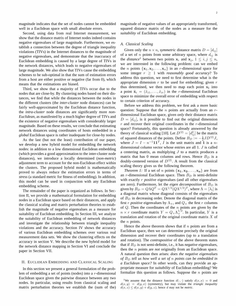
We evaluate the performance gain obtained by using thelocalized adjustment term (LAT) option in network distanceembedding. For this purpose, we compare the stress of theVL-ALL method without LAT and the VL-ALL method withLAT, where the local adjustment term is computed using allthe nodes. We vary the number of dimensions from 2 to 7. Ascan be seen in Fig. 15, the use of adjustment term (keys withLAT) reduces the stress significantly compared to the VL-All without LAT. In particular, when the original Euclideanembedding has high stress (large error), the reduction of

8It is possible that the estimated distance is negative due tonegative LAT.In this case, we use the estimation of the Euclidean part as the estimateddistance.

12

0 0.1 0.2 0.3 0.4 0.5 0.6 0.7 0.8 0.9

1

0 0.2 0.4 0.6 0.8 1

cum

ulat

ive

dist

ribut

ion

relative error

VL-All,7DVL-All,7D,SLATVL-All,2D,SLAT

(a) Relative Error

0 0.1 0.2 0.3 0.4 0.5 0.6 0.7 0.8 0.9

1

0 2 4 6 8 10 12 14 16 18

cnl

δ (ms)

7D7D,SLAT2D,SLAT

(b) CNL

0 0.1 0.2 0.3 0.4 0.5 0.6 0.7 0.8 0.9

1

0 0.2 0.4 0.6 0.8 1

cum

ulat

ive

dist

ribut

ion

rrl

VL-All,7DVL-All,7D,SLATVL-All,2D,SLAT

(c) RRL

Fig. 16. The performance of VL-All method with SLAT onKing462 data set.

0

0.1

0.2

0.3

0.4

0.5

2 3 4 5 6 7

stre

ss

number of dimensions

King462,VL-AllKing462,VL-All,LAT

King462,VL-All,SLATPlanetlab,VL-All

Planetlab,VL-All,LATPlanetlab,VL-All,SLAT

Fig. 15. Stress of Virtual landmarks method over the number of dimensions.Both LAT and SLAT options are shown together.

stress is significant, which is expected from Theorem 4. Next,we evaluate the performance of LAT using only a smallnumber of randomly selected nodes as in eq.(3); we callthis option “SLAT (Sampled LAT)”. Fig. 15 shows the stressof embedding using SLAT (keys with SLAT) over differentnumber of dimensions, where the adjustment term is computedusing the measurement to 10 randomly selected nodes. We seethat the performance between LAT and SLAT are very close.This is quite expected because the average of a randomlysampled set is an unbiased estimation of the average ofthe entire set. This result indicates that the adjustment termcan actually be computed quickly with a small number ofadditional measurements. The results also show that increasingthe dimension of the Euclidean embedding does not help verymuch; in fact, a lower dimension Euclidean embedding plusthe local adjustment terms is sufficient to improve the accuracyof the embedding significantly.

In addition to the improved overall stress, the local ad-justment terms also improve the relative errors. As an ex-ample, Fig. 16(a) compares the cumulative distribution ofthe relative errors of the VL-ALL with 7 dimensions (de-noted “VL-ALL,7D”) with that using the same method with7 dimensions plus SLAT (denoted as “VL-ALL,7D,SLAT”)and with only 2 dimensionsplus SLAT (denoted as “VL-ALL,2D,SLAT”) for the King462 data set9. The VL-ALL

9The Euclidean coordinates of the SLAT (2D+1) are the first 2 coordinatesof the Virtual Landmark 7 dimension embedding.

with 2 dimensions plus SLAT attains better performance thanthat of the pure VL-ALL with 7 dimensions. For example,90 percentile relative error of “VL-ALL,2D,SLAT” is lessthan 0.6, but that of “VL-ALL,7D” is larger than 1.0. Theperformance of “VL-ALL,2D,SLAT’ is even better than thatof “VL-ALL,7D,SLAT”, where 7 dimensions is used. Weconclude that adding a (non-Euclidean) local adjustment termis far more effective in improving the accuracy of embeddingthan adding additional dimensions. More in-depth analysisdemonstrates that the performance gain comes largely fromimproved distance estimation for nodes within the same clus-ter. However, for the metric, CNL, as can be seen in Fig. 16(b),the performance degrades with SLAT. It means that SLAToption is not good for choosing the closest node. For themetric, RRL, the performance with SLAT is a little better thanthe one without SLAT as can be seen in Fig. 16(c).

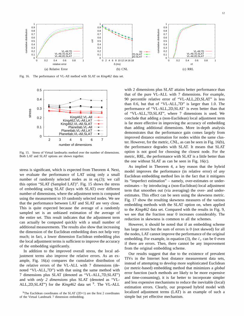
As implied in Theorem 4, a key reason that the hybridmodel improves the performance (in relative error) ofanyEuclidean embedding method lies in the fact that it mitigatesits “imperfect estimation” – namely, over-estimates or under-estimates – by introducing a (non-Euclidean) local adjustmentterm that smoothes out (via averaging) the over- and under-estimates. This effect can be seen using the skewness metric.Fig. 17 show the resulting skewness measures of the variousembedding methods with the SLAT option on, when appliedto theKing462data set. Compared with the results in Fig. 9,we see that the fraction near 0 increases considerably. Thereduction in skewness is common to all the schemes.

However, it should be noted that if an embedding schemehas large errors but the sum of errors is 0 (not skewed) for allthe nodes, LAT cannot improve the performance of the originalembedding. For example, in equation (3), theex can be 0 evenif there are errors. Then, there cannot be any improvementfrom the original embedding scheme.

Our results suggest that due to the existence of prevalentTIVs in the Internet host distance measurement data sets,instead of attempting to develop more sophisticated Euclidean(or metric-based) embedding method that minimizes aglobalerror function (such methods are likely to be more expensiveand time-consuming), it is far better to incorporate simplerand less expensive mechanisms to reduce the inevitable (local)estimation errors. Clearly, our proposed hybrid model withlocalized adjustment terms (LAT) is an example of such asimple but yet effective mechanism.

13

0

0.1

0.2

0.3

0.4

0.5

0.6

0.7

0.8

-30 -20 -10 0 10 20 30

frac

tion

skewness (ms)

GNP,SLATVL-All,SLATVivaldi,SLAT

Fig. 17. Cumulative distributions ofsx under various schemes with theSLAT option. The data set isKing462. The number of dimension is 7.

VII. C ONCLUSION

This paper investigated the suitability of embedding Internethosts into a Euclidean space given their pairwise distances(as measured by round-trip time). Using the classical scalingand matrix perturbation theories, we established that the (sumof the) magnitude ofnegativeeigenvalues of the (doubly-centered, squared) distance matrix as a measure of suitabilityof Euclidean embedding. Using data sets from real Internethost distance measurements, we illustrated that the distancematrix among Internet hosts contains negative eigenvaluesof large magnitude, implying that embedding the Internethosts in a Euclidean space would incur considerable errors.We attributed the existence of these large-magnitude negativeeigenvalues to the prevalence oftriangle inequality violations(TIVs) in the data sets. Furthermore, we demonstrated that theTIVs are likely to occurlocally, hence the distances amongthese close-by hosts cannot be estimated very accurately usinga global Euclidean embedding. In addition, increasing thedimension of embedding does not reduce the embeddingerrors.

Based on these insights, we proposed and developed a sim-ple hybrid model that incorporates a localized (non-Euclidean)adjustment term for each node on top of a low-dimensionalEuclidean coordinate system. Our hybrid model preservesthe advantages of the Euclidean coordinate systems, whileimproving their efficacy and reducing their overheads (byusing a small number of dimensions). Through both mathemat-ical analysis and experimental evaluation, our hybrid modelimproves the performance of existing embedding methodswhile using only a low dimension embedding. Lastly, ourmodel can be incorporated into any embedding system (notnecessarily Euclidean embedding).

REFERENCES

[1] S. Lee, Z.-L. Zhang, S. Sahu, and D. Saha, “On suitabilityof euclideanembedding of internet hosts,” inProc. ACM SIGMETRICS, Saint Malo,France, June 2006.

[2] T. E. Ng and H. Zhang, “Predicting Internet network distance withcoordinates-based approaches,” inProc. IEEE INFOCOM, New York,NY, June 2002.

[3] L. Tang and M. Crovella, “Virtual landmarks for the Internet,” inProceedings of the Internet Measurement Conference(IMC), Miami,Florida, Oct. 2003.

[4] H. Lim, J. C. Hou, and C.-H. Choi, “Constructing Internetcoordinatesystem based on delay measurement,” inProceedings of the InternetMeasurement Conference(IMC), Miami, Florida, Oct. 2003.

[5] F. Dabek, R. Cox, F. Kaashoek, and R. Morris, “Vivaldi: A decentralizednetwork coordinate system,” inProceedings of ACM SIGCOMM 2004,Portland, OR, Aug. 2004.

[6] M. Costa, M. Castro, A. Rowstron, and P. Key, “Pic: Practical Internetcoordinates for distance estimation,” inProceedings of InternationalConference on Distributed Computing Systems (ICDCS), Tokyo, Japan,Mar. 2004.

[7] H. Zheng, E. K. Lua, M. Pias, and T. G. Griffin, “Internet routingpolicies and round-trip-times,” inThe 6th anuual Passive and ActiveMeasurement Workshop, Boston, MA, Mar. 2005.

[8] E. K. Lua, T. Griffin, M. Pias, H. Zheng, and J. Crowcroft, “On theaccuracy of embeddings for internet coordinate systems,” in Proceedingsof the Internet Measurement Conference(IMC), Boston, MA, Apr. 2005.

[9] B. Wong, A. Slivkins, and E. G. Sirer, “Meridian: A lightweight networklocation service without virtual coordinates,” inProceedings of ACMSIGCOMM 2005, Philadelphia, PA, Aug. 2005.

[10] I. Borg and P. Groenen,Modern Multidimensional Scaling : Theory andApplications. Springer, 1997.

[11] G. H. Gulub and C. F. van Loan,Matrix Computation, 3rd ed. theJohn Hopkins University Press, 1996.

[12] T. M. Gil, F. Kaashoek, J. Li, R. Morris, and J. Stribling, “King462 dataset,” http://pdos.lcs.mit.edu/p2psim/kingdata, current year.

[13] “King2305 data set,” http://www.cs.cornell.edu/People/egs/meridian/data.php.[14] J. Stribling, “Rtt among planetlab nodes,”

http://www.pdos.lcs.mit.edu/ strib/plapp/, current year.[15] “Global nework positioning (gnp),” http://www-2.cs.cmu.edu/ euge-

neng/research/gnp/.[16] A. Gupta, “Embedding tree metrics into low-dimensional euclidean

spaces,”Discrete and Computational Geometry, vol. 24, no. 1, pp. 105–116, May 2000.

[17] “Network coordinate research at harvard,”http://www.eecs.harvard.edu/syrah/nc/.

[18] A. Y. Ng, M. I. Jordan, and Y. Weiss, “On spectral clustering : Analysisand an algorithm,”Advances in Neural Information Processing Systems(NIPS), vol. 14, 2002.

[19] D. B. West, Introduction to Graph Theory, 2nd ed. Prentice Hall.,2001.

APPENDIX

Proof of Theorem 2. First, verifying whether there exists amaximal TIV-free set of sizek among a set of nodes with a distancematrix can be done in polynomial time by enumerating all set of sizek and checking the TIVs in a non-deterministic machine. Hencethisproblem isNP .

Now we prove that the problem is NP-hard by reducing the MAX-CLIQUE problem (namely, finding the maximal clique in a graphG,a well-known NP-complete problem [19]) to the maximal TIV-freeset problem. LetG be a connected undirected graph withn > 2nodes. We assume that the size of maximal clique ofG is k > 2.(The casek = 2 is trivial, as any pair of vertices with an edge is amaximal clique.) We construct a distance matrixD = (dij) amongthe set of vertices ofG as follows, wheredij will be the defineddistance between verticesi andj. For each vertexi, we setdii = 0.For each edgeeij between verticesi and j, we setdij = 1 anddji = 1. Note that for any triangle inG, the corresponding distancesin D do not violate triangle inequality. For the pair of verticesiand j that do not have an edge between them inG, we first setdij := undefined. Now, we define all the undefineddij as follows.For an undefineddij , we computec = maxk(dik+dkj) for all k suchthat dik anddkj are already defined. If no suchc can be computedbecausedik and dkj are undefined for allk, we setc = 0. Then,we setdij := dji := c + 1. This transformation takes polynomialtime,O(n3), since there aren2 entries inD and for each entryO(n)computation is required.

It can be easily shown that that a triple of nodes(i, j, k) in G formsa triangle if and only ifi, j, andk do not violate triangle inequalitywith dij , dik, anddjk in D (we omit the detailed proof for the sake ofspace). This means that the maximal TIV-free set with the distances

14

defined asD is the maximal clique inG. We conclude that finding amaximal TIV-free set problem is NP-hard. Since maximal TIV-freeset problem is NP and NP-hard, it is NP-complete.

Proof of Lemma 1. Note thattc > ta + tb. Let (ta, tb, tc) bea metric embedding of the 3 nodes. Then, they should satisfy thetriangle inequality constraint as follows.

ta + tb ≥ tc, ta + tc ≥ tb, tb + tc ≥ ta (4)

The squared estimation error,e, in this embedding is

e = (ta − ta)2 + (tb − tb)2 + (tc − tc)

2 (5)

Let k := |ta − ta| + |tb − tb| + |tc − tc|. We now show thatk ≥ (tc − ta − tb). Supposek < (tc − ta − tb). There are 8 casesbased on the signs of(ta− ta), (tb− tb), and(tc− tc). First, considerthe case where(ta > ta), (tb > tb), and(tc > tc). Then,

k − (tc − ta − tb)

= (ta − ta) + (tb − tb) + (tc − tc) − (tc − ta − tb)

= 2(ta + tb) − ta − tb − tc

> 2(ta + tb) − ta − tb − tc

> ta + tb − tc ≥ 0

So k > (tc − ta − tb), a contradiction. It can be easily shown thatall the other 7 cases contradict, too. So we conclude thatk ≥ (tc −ta − tb).

Now, for any suchk ≥ (tc−ta−tb), consider another embedding(ta, tb, tc) such thatta = ta+ k

3, tb = tb+ k

3, andtc = tc−

k

3. Since

it can be easily shown that (ta, tb, tc) satisfies the triangle inequalityconstraint, it is a metric embedding.

Furthermore, for any suchk ≥ (tc − ta − tb), (5) is minimizedwith this embedding because

|ta − ta| = |tb − tb| = |tc − tc| =k

3(6)

Therefore,e ≥ ( k

3)2 + ( k

3)2 + ( k

3)2 = k2

3≥ (tc−ta−tb)2

3.

Proof of Theorem 3 Let E be the sum of squared error ofn

nodes.E =∑

i(di − di)

2, wheredi is a distance between a pairof nodes (calledi) and di is the embedded distance of the pairi.There aren(n − 1)/2 pairs. Since there aren(n − 1)(n − 2)/6

triples amongn nodes,E can be rewritten by the triples of nodesas follows.E = 1

n−2

∑

t∈T

(

(ta − ta)2 + (tb − tb)2 + (tc − tc)

2)

,whereT is the set of triples andta, tb, andtc are the three distances ofa triplet, andta, tb, andtc are the corresponding embedded distances.Clearly, E ≥ 1

n−2

∑

t∈V

(

(ta − ta)2 + (tb − tb)2 + (tc − tc)

2)

,whereV ⊂ T is the set of TIV triples. From Lemma 1, we haveE ≥ 1

3(n−2)

∑

t∈V(tc − ta − tb)

2.

Proof of Theorem 4 We just describe a sketchy of the proof.Let s1 be the stress of using the pure Euclidean based scheme. Lets2 be the stress of using the pure Euclidean based scheme with theadjustment term.

s21 =

∑

x,y(dxy − dE

xy)2∑

xyd2

xy

(7)

s22 =

∑

x,y(dxy − dE

xy − ex − ey)2∑

x,yd2

xy

(8)

Since the denominators are the same, we compute(∑

x,yd2

xy)(s21 − s2

2) to computes21 − s2

2.

(∑

x,y

d2xy)(s2

1 − s22)

=∑

x,y

(dxy − dExy)2 −

∑

x,y

(dxy − dExy − ex − ey)2

Using (2) and reformatting the formula, the final result can beeasily obtained.

Sanghwan Leereceived the BS and MS degree incomputer science from Seoul National University,Seoul, Korea, in 1993 and 1995 respectively, and thePh.D. degree in computer science and engineeringfrom the University of Minnesota, Minneapolis, in2005.

Dr. Lee is currently an Assistant Professor atKookmin University, Seoul, Korea. From June 2005to February 2006, he worked at IBM T.J. WatsonResearch Center, Hawthorne, NY. His main researchinterest is theory and services in the Internet. He is

currently applying the embedding schemes to a live peer to peer multimediastreaming system to see the real impact of the accuracy on theapplicationperspective performance.

Zhi-Li Zhang received the Ph.D. degree in com-puter science from the University of Massachusetts,Boston, in 1997.

In 1997, he joined the Computer Science andEngineering Faculty, University of Minnesota, Min-neapolis, where he is currently a Full Professor.

Dr. Zhang was a recipient of the National ScienceFoundation CAREER Award in 1997. He has alsobeen awarded the prestigious McKnight Land-GrantProfessorship and George Taylor Distinguished Re-search Award at the University of Minnesota, and the

Miller Visiting Professorship at Miller Institute for Basic Sciences, Universityof California, Berkeley. He is a co-recipient of an ACM SIGMETRICS BestPaper Award and an IEEE International Conference on NetworkProtocols(ICNP) Best Paper Award.

Sambit Sahu is a research staff member in theNetworking Software and Services Group. He re-ceived a Ph.D. degree in computer science from theUniversity of Massachusetts at Amherst in 2001.He joined IBM in 2001. His research has focusedon overlay-based communication, network configu-ration management, content distribution architecture,and design and analysis of high-performance net-work protocols. Dr. Sahu has published a number ofpapers in the areas of differentiated services, mul-timedia, overlay-based communication, and network

management and has over 20 patents filed in these areas.

Debanjan Saha is with the Security, Privacy, andNetworking Department at IBM Research. He leadsa group of researchers working on different aspectsof network software and services. He received aB.Tech. degree in computer science and engineeringfrom the Indian Institute of Technology in 1990, andM.S. and Ph.D. degrees in computer science fromthe University of Maryland at College Park in 1992and 1995, respectively. Dr. Saha has authored morethan 50 papers and standards contributions and is afrequent speaker at academic and industry events.

He serves regularly on the executive and technical committees of majornetworking conferences.