Journal of Glaciology, Vol. 61 , No. 229, 2015 doi: 10.3189/2015JoG15J141 1015

Ice thickness distribution and hydrothermal structure of Elfenbeinbreen and Sveigbreen, eastern Spitsbergen, Svalbard

INTRODUCTION In recent decades, Svalbard glaciers have been widely radio-echo sounded. The earliest extensive surveys of ice thickness were the airborne echo soundings carried out in the 1970s and 1980s (Macheret and Zhuravlev, 1982; Dowdeswell and others, 1984). These studies used low-accuracy radar and positioning systems and mostly consisted of a single profile along the centre line of each glacier. Subsequent radar campaigns, mostly ground-based but sometimes also air­borne, used increasingly improved radar and positioning systems providing a wider coverage of the glacier surfaces by radar profiles. A complete summary of glaciers on Svalbard with readily available radio-echo sounded ice-thickness data can be found in Martín-Español and others (2015).

Despite the rather high number of radio-echo sounding studies, the eastern coast of central Spitsbergen is still devoid of ice-thickness measurements. With the aim of partly filling this gap, we carried out a radio-echo sounding campaign on Elfenbeinbreen and Sveigbreen (Fig. 1), with the main results reported in this correspondence. With this study, we also aim at contributing to the community effort of making available the data on volume and ice-thickness distribution of glaciers around the globe (Gärtner-Roer and others, 2014).

STUDY SITE, RADAR CAMPAIGN AND GPR DATA

PROCESSING

Elfenbeinbreen and Sveigbreen (Fig. 1; Table 1) are two land-terminating valley glaciers in Sabine Land, eastern Spitsbergen, Svalbard. Elfenbeinbreen is one of the major outlets of Nordmannsfonna. It drains the ice field south­wards into Agardhdalen val ley. Sveigbreen shows a comparable setting. It is one of the major outlets of Hellefonna and drains eastwards, also into Agardhdalen. Both glaciers are of comparable size (~30-40 km2 ; Table 2) wi th Elfenbeinbreen being the larger. They both extend from 600-700 m a.s.l. almost down to sea level and show a small average slope (Table 1).

Table 1 . Key data for Elfenbeinbreen and Sveigbreen. The IDs of the glaciers are given with respect to the Randolph Glacier Inventory version 4.0 (RGI40; Pfeffer and others, 2014), the Global Land Ice Measurements from Space (GLIMS) database (https://nsidc.org/ glims/), and the Inventory of Svalbard radio-echo sounded (ISRES) glaciers (http://svalglac.eu). Horizontal characteristic glacier shape is defined as average width divided by length along central flowline

Glacier Elfenbeinbreen Sveigbreen

RGI40 ID GLIMS ID ISRES ID Central latitude (°) Central longitude (°) Elevation range (ma.s.l.) Mean slope (°) Horizontal glacier shape

07.00428 07.00409 018206E, 78185N 017698E, 78107N

156 157 78.1851 78.1071 18.2064 17.6978 50-700 50-600

0.06 0.05

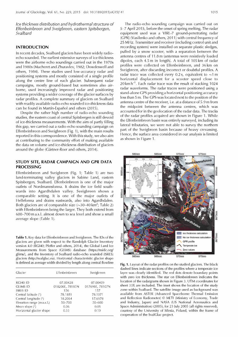
The radio-echo sounding campaign was carried out on 5-7 April 2015, before the onset of spring melting. The radar equipment used was a VIRL-7 ground-penetrating radar (GPR) (Vasilenko and others, 2011) with central frequency of 25 MHz. Transmitter and receiver (including control unit and recording system) were installed on separate plastic sledges, pulled by a snow scooter, wi th a separation between the antenna centres of 11.8 m (antennas were resistively loaded dipoles, each 4.5 m in length). A total of 105 km of radar profiles were collected on Elfenbeinbreen, and 3 6 k m on Sveigbreen, after discarding incorrect or doubtful profiles. A radar trace was collected every 0.2 s, equivalent to ~ 1 m horizontal displacement for a scooter speed close to 20 km h–1. Each radar trace was the result of stacking 1024 radar waveforms. The radar traces were positioned using a stand-alone GPS providing a horizontal positioning accuracy less than 5 m. The GPS was located next to the position of the antenna centre of the receiver, i.e. ata distance of 5.9 m from the midpoint between the antenna centres, which was accounted for in the geolocation of the radar data. The tracks of the radar profiles acquired are shown in Figure 1. Whi le the Elfenbeinbreen basin was entirely surveyed, including its lateral tributaries, we were not able to survey the northern part of the Sveigbreen basin because of heavy crevassing. Hence, the surface area considered in our analysis is l imited as shown in Figure 1.

0.33 0.19

Fig. 1 . Layout of the radar profiles on the studied glaciers. The black dashed lines indicate sections of the profiles where a temperate ice layer was clearly identified. The red dots denote boundary points with zero ice thickness. The star on Elfenbeinbreen indicates the location of the radargrams shown in Figure 3. UTM coordinates for sheet 33X are included. The inset shows the location of the study zone within Svalbard. The satellite image used as background was available from ASTER (Advanced Spaceborne Thermal Emission and Reflection Radiometer) © METI (Ministry of Economy, Trade and Industry, Japan) and NASA (US National Aeronautics and Space Administration) (2005), for 23 July 2005 (all rights reserved), courtesy of the University of Silesia, Poland, within the frame of cooperation of the SvalGlac project.

1016 Navarro and others: Correspondence

Fig. 2. Ice-thickness maps of Sveigbreen (a) and Elfenbeinbreen (b). Contour interval is 20 m. UTM coordinates for sheet 33X are shown.

The radar data were processed using the commercial software package RadExPro, by GDS Production (Kulnitsky and others, 2000). The main processing steps consisted of bandpass fi ltering, normal moveout correction, amplitude correction and Stolt two-dimensional F-K migration. De-convolution was not used since our pulse duration is small (~25 ns), so there is no need to shorten it. The picking of the transmitted pulse and the bed return was done manually. To improve the detection of zero times, a Hilbert transform was applied upon filtering. The absolute value of the Hilbert transform of the radar signal is proportional to the radio-wave energy, including both magnetic and electric fields. This procedure results in small picking errors of the order of the sampling period (2.5 ns), equivalent to ~ 0 . 4 m . For the time-to-thickness conversion we used a constant radio-wave velocity of 0.168mns–1 , taking into account previous common-midpoint measurements on Svalbard, the thick­ness of the glaciers under study and the fact that the measurements were made in early spring before the onset of melting (Martín-Español and others, 2013; Navarro and others, 2014). Navarro and others (2014) show that the use

of a constant radio-wave velocity, if selected on the basis of regional column-averaged measurements and taking into account the glacier size and morphology, has little influence on the average ice-thickness estimates.

ICE-THICKNESS D I S T R I B U T I O N A N D

H Y D R O T H E R M A L STRUCTURE

Based on 76164 (Elfenbeinbreen) and 21 306 (Sveigbreen) ice-thickness data points picked from the radargrams, plus 404 (Elfenbeinbreen) and 556 (Sveigbreen) zero-thickness data points on glacier boundaries wi th contact between glacier ice and rock/ground (at glacier side-walls or snout), we constructed the ice-thickness maps shown in Figure 2. The interpolation, over a regular grid of 100 m x 100 m, was done using anisotropic ordinary kriging with a spherical variogram.

Mean ice thickness is slightly higher for Elfenbeinbreen than for Sveigbreen, with just a ~ 1 5 % difference between the two glaciers (Table 2). The maximum ice thickness of Elfenbeinbreen is close to 300 m whi le that of Sveigbreen is

Table 2. Area, volume, and mean and maximum ice thickness of the studied glaciers. The area shown for Sveigbreen is smaller than that in the Randolph Glacier Inventory, because a portion of this glacier had to be excluded from the echo sounding (cf. Fig. 1). The errors in area correspond to 8%, based on the accuracy study for Svalbard glaciers by Nuth and others (2013). The errors in volume involve both errors in ice thickness and errors in area, and are estimated as described in Navarro and others (2014). In this particular case, both error components contributed similar shares to the total error in volume. The relative errors in volume are 5 .1% for Elfenbeinbreen and 5.3% for Sveigbreen

Glacier Area

km2

Volume

km3

H

m

Hmax

m

Elfenbeinbreen

Sveigbreen

39.96 ± 3 . 2 0

28.59 ±2 .29

3.368 ±0.173

2.004 ±0 .107

85.28 ±8 .84

73.58 ± 7.42

285.12 ± 6.62

212.43 ± 5.42

Navarro and others: Correspondence 1017

Fig. 3. Sample radargrams corresponding to two intersecting profiles in the ablation zone of the main trunk of Elfenbeinbreen (location indicated by a star in Fig. 1): (a) profile along the central flowline; (b) transverse profile. Both panels are at the same scale. The arrows indicate the location of the intersection between the two profiles. The radargrams are not migrated, to mark the difference between cold and temperate ice. The zone showing abundant diffractions corresponds to temperate ice (~50m thick in the deepest part of the transverse profile, also seen in the central part of the longitudinal profile), while the zones with ‘cleaner’ image (free from diffractions) correspond to cold ice. The stacks of narrow hyperbolae indicate the presence of surface crevasses.

considerably smaller at just over 2 0 0 m (Table 2). Table 2 also shows the glacier areas and the computed volumes. When computing volumes, those of the unsurveyed small tributary basins in the upper reaches of Sveigbreen were approximated using the tributary thickness function for Svalbard glaciers described in Navarro and others (2014). The volume data show that Elfenbeinbreen contains a ~ 6 5 % larger ice volume than Sveigbreen, though we should keep in mind that a portion (~25%) of the Sveigbreen basin was excluded from the computations.

The radargrams depict a clear polythermal glacier structure (Fig. 3), though the volume of cold ice is larger than that usually found by the authors for glaciers of similar size in central and western Nordenskiöld Land (Martín-Español and others, 2013) and in Wedel Jarlsberg Land (Navarro and others, 2014). The volume of cold ice is especially large for Elfenbeinbreen and its tributary glaciers; the latter mostly consist of cold ice. The thickness of the upper cold-ice layer of Elfenbeinbreen varies between roughly 80 and 2 5 0 m , though it is generally ~ 1 2 0 - 1 5 0 m . Where the glacier thickness is lower than ~ 1 0 0 m, the entire ice column most often consists only of cold ice. By contrast, the cold layer of Sveigbreen is much thinner, typically 6 0 -80 m, often of similar thickness to (or sometimes thinner than) the temperate layer beneath. The lower ablation zone of Sveigbreen mostly consists of cold ice, though it could be warm-based, and the glacier snout is likely frozen to the bed. In Figure 1 we show the sections of the radar profiles where a temperate ice layer has been clearly identified. Comparing Figures 1 and 2, it can be seen that, in general, the temperate ice appears in the zones wi th thickest ice. An exception to this is the zone of thickest ice of Elfenbein­breen, which appears to consist mostly of cold ice, though it could be temperate-based.

The firn layer is particularly thick in the uppermost part of Elfenbeinbreen, reaching ~ 4 0 m (assuming a radio-wave velocity in firn of 0.190mns–1) in the transition zone from Elfenbeinbreen to Nordmannsfonna. Due to the proximity of the two glaciers, the general ly thicker f i rn layer of Elfenbeinbreen, compared wi th Sveigbreen, is unlikely to

be due to climate. Instead, snowdrift processes are known to have significant impact on local- to regional-scale snow-cover patterns on Svalbard (e.g. Sauter and others, 2013) and could be seen as a potential explanation for the thick firn cover in the upper reaches of Elfenbeinbreen. Consider­ing katabatic airflow, the glacier is situated downwind of the vast accumulation areas of Nordmannsfonna. As these areas form an abundant source region for drifting snow, additional accumulation amounts along Elfenbeinbreen are conceiv­able. Part of this observed difference in firn thickness between the two glaciers could be simply apparent, as the portion of Sveigbreen excluded from our study mostly corresponds to its accumulation zone, in the transition zone from Sveigbreen to Hellefonna. We note, anyway, that Hellefonna is much smaller in area than Nordmannsfonna.

In any case, the observed differences in thickness of the firn layer in the two glaciers do not explain the differences in thickness of the cold and temperate ice layers, as the latter differences are also present in the main trunks of both glaciers. Nor do the differences in ice thickness provide a satisfactory explanation. Sveigbreen, being thinner, might be expected to have a larger proportion of cold ice; this is not the case. Moreover, its slightly gentler slopes than those of Elfenbeinbreen imply a larger driving stress, which would likely result in lower velocities and hence lower strain heating, thus contributing to a smaller proportion of temperate ice. Such intriguing characteristics call for further research, with focus on the accumulation pattern and the dynamics of these glaciers.

ACKNOWLEDGEMENTS

Fieldwork was done with permission of Svalbard Governor (Permit Reference: 2013/01196-5) and documented in the Research in Svalbard database (RiS ID: 6726). This research was supported by grant No. MO2653/1-1 of the German Research Foundation (DFG) and by Project CTM2011-28980 from the Spanish National Plan for R&D. We thank the reviewers Yuri Macheret and Rickard Pettersson for suggestions to improve this correspondence.

1018 Navarro and others: Correspondence

Department of Mathematics, Francisco NAVARRO Applied Information Technologies and Communications, Universidad Politécnica de Madrid, Madrid, Spain E-mail: francisco.navarro@upm.es

Department of Geography, Rebecca MÖLLER RWTH Aachen University, Aachen, Germany

Institute of Industrial Research Evgeny VASILENKO Akadempribor, Academy of Sciences of Uzbekistan, Tashkent, Uzbekistan

School of Geographical Sciences, Alba MARTÍN-ESPAÑOL University of Bristol, Bristol, UK

Department of Mathematics, Roman FINKELNBURG Applied Information Technologies and Communications, Universidad Politécnica de Madrid, Madrid, Spain

Department of Geography, Marco MÖLLER RWTH Aachen University, Aachen, Germany

19 September 2015

REFERENCES

Dowdeswell JA, Drewry DJ, Liestøl O and Orheim O (1984) Radio echo-sounding of Spitsbergen glaciers: problems in the inter­pretation of layer and bottom returns. J. Glaciol., 30(104), 16–21

Gärtner-Roer I, Naegeli K, Huss M, Knecht T, Machguth H and Zemp M (2014) A database of worldwide glacier thickness observations. Global Planet. Change, 122, 330–344 (doi: 10.1016/j.gloplacha.2014.09.003)

Kulnitsky LM, Gofman PA and Tokarev MY (2000) Matematiches-kaya obrabotka dannykh georadiolokatsii i systema RADEXPRO [Mathematical processing of georadar data and RADEXPRO system]. Razv. Okhrana Nedr, 3 , 6–11

Macheret YuYa and Zhuravlev AB (1982) Radio echo-sounding of Svalbard glaciers. J. Glaciol., 28(99), 295–314

Martín-Español and 7 others (2013) Radio-echo sounding and ice volume estimates of western Nordenskiold Land glaciers, Svalbard. Ann. Glaciol., 54(64), 211–217 (doi: 10.3189/ 2013AoG64A109)

Martín-Español A, Navarro FJ, Otero J, Lapazaran JJ and Błaszczyk M (2015) Estimate of the total volume of Svalbard glaciers, and their potential contribution to sea-level rise, using new regionally based scaling relationships. J. Glaciol., 61(225), 29–41 (doi: 10.3189/2015JoG14J159)

Navarro FJ and 6 others (2014) Ice volume estimates from ground-penetrating radar surveys, Wedel Jarlsberg land glaciers, Svalbard. Arct. Antarct. Alp. Res., 46(2), 394–406 (doi: 10.1657/ 1938-4246-46.2.394)

Nuth C and 7 others (2013) Decadal changes from a multi-temporal glacier inventory of Svalbard. Cryosphere, 7(5), 1603–1621 (doi: 10.5194/tc-7-1603-2013)

Pfeffer WT and 19 others (2014) The Randolph Glacier Inventory: a globally complete inventory of glaciers. J. Glaciol., 60(221), 537–552 (doi: 10.3189/2014JoG13J176)

Sauter T, Möller M, Finkelnburg R, Grabiec M, Scherer D and Schneider C (2013) Snowdrift modelling for the Vestfonna ice cap, north-eastern Svalbard. Cryosphere, 7(4), 1287–1301 (doi: 10.5194/tc-7-1287-2013)

Vasilenko EV, Machío F, Lapazaran JJ, Navarro FJ and Frolovskiy K (2011) A compact lightweight multipurpose ground-penetrating radar for glaciological applications. J. Glaciol., 57(206), 1113–1118 (doi: 10.3189/002214311798843430)