ices wki 3 report 2017 - welcome to ices reports/expert group...ices wkirish3 report 2017 ices b...
TRANSCRIPT

ICES WKIRISH3 REPORT 2017 ICES BENCHMARK STEERING GROUP COMMITTEE
ICES CM 2017/BSG:01
REF. ACOM, SCICOM, BSG, WKIRISH4
Report of the Benchmark Workshop on the Irish Sea Ecosystem (WKIrish3)
30 January–3 February 2017
Galway, Ireland

International Council for the Exploration of the Sea Conseil International pour l’Exploration de la Mer
H. C. Andersens Boulevard 44–46 DK-1553 Copenhagen V Denmark Telephone (+45) 33 38 67 00 Telefax (+45) 33 93 42 15 www.ices.dk [email protected]
Recommended format for purposes of citation:
ICES. 2017. Report of the Benchmark Workshop on the Irish Sea Ecosystem (WKIrish3), 30 January–3 February 2017, Galway, Ireland. ICES CM 2017/BSG:01. 165 pp.
For permission to reproduce material from this publication, please apply to the Gen-eral Secretary.
The document is a report of an Expert Group under the auspices of the International Council for the Exploration of the Sea and does not necessarily represent the views of the Council.
© 2017 International Council for the Exploration of the Sea

ICES WKIrish3 REPORT 2017 | i
Contents
Executive summary ................................................................................................................ 4
1 Opening of the meeting ................................................................................................ 5
2 Derivation of natural mortality (M) ........................................................................... 7
3 Irish Sea herring........................................................................................................... 11
4 Irish Sea cod .................................................................................................................. 12
4.1 Issue list ................................................................................................................ 12 4.2 Data ....................................................................................................................... 12
4.2.1 Stock identity and migration ................................................................ 12 4.2.2 Life-history data ..................................................................................... 12 4.2.3 Fishery-dependent data ........................................................................ 12 4.2.4 Fishery-independent data ..................................................................... 12 4.2.5 Environmental drivers and ecosystem impacts ................................. 12
4.3 Assessment and forecast .................................................................................... 12 4.3.1 Assessment models and runs ............................................................... 12 4.3.2 Final assessment model run ................................................................. 21 4.3.3 Short-term forecast ................................................................................ 33
4.4 Reference points .................................................................................................. 34
4.5 Future research and data requirements ........................................................... 34
4.6 Multispecies information: WKIrish4 ................................................................ 34
5 Irish Sea haddock ........................................................................................................ 35
5.1 Issue list ................................................................................................................ 35 5.2 Data ....................................................................................................................... 35
5.2.1 Stock identity and migration ................................................................ 35 5.2.2 Life-history data ..................................................................................... 35 5.2.3 Other biological information ................................................................ 35 5.2.4 Fishery-dependent data ........................................................................ 36 5.2.5 Fishery-independent data ..................................................................... 36 5.2.6 Environmental drivers and ecosystem impacts ................................. 36
5.3 Assessment and forecast .................................................................................... 36 5.3.1 Assessment models and runs ............................................................... 36 5.3.2 Final assessment model run ................................................................. 46 5.3.3 Short-term forecast ................................................................................ 48
5.4 Reference points .................................................................................................. 48
5.5 Future research and data requirements ........................................................... 50 5.6 Multispecies information: WKIrish4 ................................................................ 50
6 Irish Sea whiting .......................................................................................................... 51

ii | ICES WKIrish3 REPORT 2017
6.1 Issue list ................................................................................................................ 51 6.2 Data ....................................................................................................................... 51
6.2.1 Stock identity and migration ................................................................ 51 6.2.2 Life-history data ..................................................................................... 51 6.2.3 Other biological information ................................................................ 51 6.2.4 Fishery-dependent data ........................................................................ 51 6.2.5 Fishery-independent data ..................................................................... 51 6.2.6 Environmental drivers and ecosystem impacts ................................. 52
6.3 Assessment and forecast .................................................................................... 52 6.3.1 Assessment models and runs ............................................................... 52 6.3.2 Final assessment model run ................................................................. 56 6.3.3 Short-term forecast ................................................................................ 57
6.4 Reference points .................................................................................................. 58
6.5 Future research and data requirements ........................................................... 58
6.6 Multispecies information: WKIrish4 ................................................................ 59
7 Irish Sea plaice ............................................................................................................. 60
7.1 Issue list ................................................................................................................ 60
7.2 Data ....................................................................................................................... 60 7.2.1 Stock identity and migration ................................................................ 60 7.2.2 Life-history data ..................................................................................... 60 7.2.3 Other biological information ................................................................ 60 7.2.4 Fishery-dependent data ........................................................................ 60 7.2.5 Fishery-independent data ..................................................................... 61 7.2.6 Environmental drivers and ecosystem impacts ................................. 61
7.3 Assessment and forecast .................................................................................... 61 7.3.1 Assessment models and runs ............................................................... 61 7.3.2 Final assessment model run ................................................................. 63 7.3.3 Short-term forecast ................................................................................ 64
7.4 Reference points .................................................................................................. 64 7.5 Future research and data requirements ........................................................... 65
7.6 Multispecies information: WKIrish4 ................................................................ 65
Annex 1: Participants list ...................................................................................... 74
Annex 2: Agenda .................................................................................................... 77
Annex 3: Radiocarbon (14C) activities in gadoid Otoliths............................... 78
Annex 4: Reconstructing Irish Sea plaice discard numbers ........................... 80
Annex 5: Plaice in 7.a reference points .............................................................. 95
Annex 6: Diagnostics and stock summary plots ............................................ 101
Annex 7: Whiting reference points ................................................................... 125
Annex 8: Cod reference points .......................................................................... 142

ICES WKIrish3 REPORT 2017 | iii
Annex 9: Haddock reference points ................................................................. 154
Annex 10: Stock Annexes ..................................................................................... 165
Annex 11: Summary report from external panel .............................................. 166

4 | ICES WKIrish3 REPORT 2017
Executive summary
The Stock Assessment Workshop for Irish Sea stocks (WKIrish3), chaired by External Chair Daniel Howell, Norway and ICES Chair Hans Gerritsen, Ireland, and attended by invited external experts Jim Ianelli, US, and Rebecca Lauerburg, Germany met in Galway, Ireland, 30 January–3 February 2017. As part of the WKIrish regional benchmark process, WKIrish3 built on the conclusions and recommendations of the Scoping Workshop (WKIrish1) and the Data Evaluation Workshop (WKIrish2).
The objectives of the workshop were to develop methods to determine stock status and short-term outlook and to propose biological reference points for the Irish Sea stocks of cod, haddock, herring, plaice and whiting.
The meeting was mainly conducted through plenary sessions with some time sched-uled to address feedback given by the group. The report sections are structured along the ToRs of the workshop as well as the headings in the stock annex.
The main outcomes of the workshop are as follows:
• Cod: ASAP model accepted, new reference points proposed. This will form the basis of the advice for 2018.
• Haddock: ASAP model accepted, new reference points proposed. Shortly after the workshop ended, the advice for 2017 was re-issued, based on the new method and reference points.
• Whiting: ASAP model accepted, new reference points proposed. This will form the basis of the advice for 2018.
• Plaice: SAM model accepted by correspondence, shortly after the meeting, new reference points proposed. This will form the basis of the advice for 2018.
• Herring: SAM model rejected. No new reference points proposed. WKIrish3 recommends that the remaining issues are addressed before the assessment working group (HAWG) through an inter-benchmark.

ICES WKIrish3 REPORT 2017 | 5
1 Opening of the meeting
The Stock Assessment Workshop for Irish Sea stocks (WKIrish3), chaired by External Chair Daniel Howell, Norway and ICES Chair Hans Gerritsen, Ireland, and attended by invited external experts Jim Ianelli, US, and Rebecca Lauerburg, Germany met in Galway, Ireland, 30 January–3 February 2017.
As part of the WKIrish regional benchmark process, WKIrish3 will work building on the conclusions and recommendations of the Scoping Workshop (WKIrish1) and the Data Evaluation Workshop (WKIrish2), to:
a ) Evaluate the appropriateness of data and methods to determine stock sta-tus and investigate methods for short-term outlook for the stocks listed in the table below. The evaluation shall include consideration of (while pay-ing particular attention to the conclusions and recommendations of WKIrish 1 and 2): i ) Stock identity and migration issues; ii ) Life-history data; iii ) Fishery-dependent and fishery-independent data, also including rec-
reational fisheries; iv ) Further inclusion of environmental drivers, multispecies information,
and ecosystem impacts for stock dynamics in the assessments and out-look.
b ) Agree and document the preferred method for evaluating stock status and (where applicable) short-term forecast and update the stock annex as ap-propriate. Knowledge of environmental drivers, including multispecies in-teractions, and ecosystem impacts should be integrated in the methodology.
If no analytical assessment method can be agreed, then an alternative method (the former method, or following the ICES approach for stocks without ana-lytical assessments) should be put forward;
c ) Evaluate the possible implications for biological reference points, when new standard analyses methods are proposed. Re-examine and update, if necessary, MSY and PA reference points according to ICES guidelines (see reports of WKMSYREF3, WKMSYREF4 and ACOMs Technical document on reference points);
d ) Develop recommendations for future improving of the assessment meth-odology and data collection;
e ) Identify aspects that require special attention by the ongoing Irish Sea re-gional benchmark process, in particular pertaining to the development of integrated multispecies and ecosystem advice (to culminate in the synthe-sis workshop WKIrish4).
f ) Ensure that relevant work is prepared in advance of the meeting, as the meeting should mainly focus on evaluating and reviewing the work. The main aspects of the work should be presented as working documents and be ready at least seven days prior to the start of the meeting.

6 | ICES WKIrish3 REPORT 2017
STOCKS STOCK LEADER
cod-27.7 Pia Schuchert
had.27.7a Mathieu Lundy
her.27.nirs Pieter-Jan Schön
ple.27.7a Timothy Earl
whg.27.7a Sara-Jane Moore / Colm Lordan
The meeting was mainly conducted through plenary sessions with some time sched-uled to address feedback given by the group. The external chair coordinated the in-put of the external experts and took responsibility of the technical chairing during the meeting. The ICES chair focused on the preparation before the meeting as well as the finalisation of the report.
The report sections are structured along the ToRs of the workshop as well as the headings in the stock annex.

ICES WKIrish3 REPORT 2017 | 7
2 Derivation of natural mortality (M)
Drivers for focus on M estimates
Natural mortality is, along with the shape of the stock–recruit relationship, a key var-iable and source of uncertainty in estimation of MSY reference points and associated FMSY catch forecasts. Estimates of recruitment and biomass from catch-based assess-ments inflate substantially as input M values are increased, and fishing mortality es-timates are consequently reduced for a given catch. Incorrect M values are a problem if the assessment model estimates of abundance are being treated as absolute, for ex-ample to compute total food consumption by the stock. As the next phase (WKIrish4) in the Irish Sea benchmark process will run ecosystem models which require infor-mation on fishery selectivity and biomass from single-species assessments, WKIrish participants felt it was desirable to carry out these assessments using values or ranges of values of M, and age dependence of M, that are likely to encompass the true values and for which there is evidence to help bound the plausible ranges. Previous ICES assessments of Irish Sea cod, haddock, whiting and plaice have used age and year invariant values of M (0.2 for gadoids; 0.12 for plaice).
M in herring
There are no direct estimates of M for Irish Sea herring. Age-dependent estimates of M for North Sea herring from the stochastic multispecies assessment model (SMS) runs for the North Sea have been used in the Irish Sea herring stock assessment for many years (Table 2.1). There are no data to indicate if M is likely to be similar in the two areas, although differences in life history (growth, maturity, maximum observed age, etc.) could be examined.
Table 2.1. Mean M-at-age for cod, haddock and whiting since 2000 given by North Sea SMS key runs (ICES, WGSAM) and reported by the ICES North Sea assessment working group (WGNSSK) in 2016. Herring figures are for the North Sea stock from the same model, but as re-ported by the ICES Herring Assessment WG as being used for Irish Sea herring.
AGE COD HADDOCK WHITING HERRING
0 1.172
1 1.180 1.272 1.313 0.787
2 0.888 0.495 0.729 0.380
3 0.234 0.321 0.610 0.353
4 0.200 0.294 0.604 0.335
5 0.200 0.276 0.568 0.315
6 0.200 0.236 0.568 0.311
7 0.200 0.216 0.568 0.304
M in plaice
The M value used for many years by ICES for Irish Sea plaice was apparently based on statistical modelling of data from tagging studies that were carried out in the Irish Sea between the 1960s and 1980s (Siddeek, 1989). The annual M values derived by Siddeek were 0.17 (SE 0.06) for males and 0.11 (SE 0.08) for females. Estimates using data only for mature male plaice were lower, indicating an age or size dependence. The 1989 Siddeek paper states that the less precise estimate of M for females, and

8 | ICES WKIrish3 REPORT 2017
higher M values obtained by applying traditional methods to the same dataset, indi-cated that a value of 0.2 is more appropriate to both sexes, which is almost double the currently used value. WKIrish could not evaluate the potential for bias in these esti-mates for plaice.
M in cod, haddock and whiting
For Irish Sea cod, haddock, whiting and herring, there are no direct estimates of M from tagging, multispecies assessments or other methods. All three of the gadoid species show very steep age profiles in fishery and survey catches, and apparent short lifespans. Evidence on age dependence and magnitude of M for other stocks of these species can be obtained from the SMS model key runs for the North Sea. The stocks of cod, haddock and whiting in the North Sea show M ~1.2 at age 1, with steep decline up to age 3 (Table 2.1). From age 3, the M for cod and haddock is 0.2–0.3, close to or just above the “traditional” value of 0.2 previously used as a year- and age-invariant value for assessments of the three gadoid species in the Irish Sea. The SMS estimate of M for whiting remains relatively high at 0.6 from age 3 onwards. There are differences in predator populations in the North and Irish Seas, and sea temperatures in the Irish Sea (and more southerly Celtic Sea) are seasonally at or near the upper range for North Atlantic cod. Fast initial growth and early maturity are features of Irish Sea cod, haddock and whiting. M-at-age for these stocks could poten-tially be higher than in the North Sea. North Sea plaice are not included in the SMS model.
Life-history based inferences on M
In the absence of multispecies model estimates of M for Irish Sea gadoid and plaice stocks, and poor understanding of biases in the plaice tagging estimates of M, WKIrish2 explored possible M values given by a wide range of life-history based methods, including those such as from Lorenzen (1996) giving age-dependent values. These methods use one or more stock-specific datasets on size-at-age, growth param-eters, maturity and maximum observed ages. The methods and results are described in detail in the WKIrish2 data evaluation workshop report, and values considered by WKIrish3 are described in the separate stock sections of the present report.
Brodziak et al. (2009) reviewed the use of maximum observed age and life-history parameters for deriving plausible size/age-dependent or age-invariant natural mor-tality rate for fish and invertebrate fishery resources. Empirical evidence and ecologi-cal theory indicated that M scales with body mass or size, and that for a given species, early life-history stages experience higher M than juvenile stages which, in turn, experience higher M than mature adults. Brodziak et al. note that the traditional assumption of a constant M may be appropriate when only mature fish are of explicit interest in the assessment, but when juvenile fish need to be modelled explicitly (e.g. because these juveniles are targeted in a fishery or caught as bycatch), then size de-pendence in M should be incorporated into the assessment application, for example, by means of a Lorenzen (1996) curve.
Also, the size-dependent mortality model for juveniles may be extended into the adult age groups, or combined with either a constant adult M or a more complex model for adults that allows for increasing M at age due to reproduction or senes-cence. Brodziak et al. suggest that, where multiple estimates of M are available, aver-aging the set of candidate estimates is considered good practice, unless a single best value can be identified based on relative credibility or goodness-of-fit to observed

ICES WKIrish3 REPORT 2017 | 9
data; however it is important to characterize the variability of estimates of M for stock assessment applications.
A more recent evaluation of the predictive performance of empirical estimators of natural mortality rate, using information on over 200 fish species, is presented by Then et al. (2015). They evaluated estimators based on various combinations of max-imum age (tmax), growth parameters, and water temperature by seeing how well these estimators matched 200 independent, direct estimates of M. They concluded that a tmax based estimator performs the best among all estimators evaluated. The tmax-based estimators in turn performed better than the Alverson–Carney (1975) method based on tmax and the von Bertalanffy K coefficient, Pauly’s (1980) method based on growth parameters and water temperature and methods based just on K. Based on cross-validation prediction error, model residual patterns, model parsimony, and biological considerations, they recommend the use of a tmax based estimator (M = 4.899tmax −0.916, prediction error = 0.32) when possible and a growth-based method (M = 4.118K0.73 Linf−0.33,prediction error = 0.6) otherwise.
Evidence to help bound plausible ranges of M
A wide range of values are given by life-history methods for each stock, and there is very little information to bound the range of plausible values. North Sea SMS esti-mates of M may not reflect the values in the Irish Sea due to differences in the ecosys-tems. Overestimation of M carries high risk because M values are positively correlated with both the assessment model estimates of biomass and the derived val-ues of FMSY. Since changes in the input M values translate into changes in biomass across the age ranges affected, this offers a possibility to use fishery-independent survey estimates of biomass to identify M vectors that lead to assessment model es-timates of SSB in the same biomass range. This is not feasible from trawl surveys without knowledge of the true catchability at-age, but could potentially be done us-ing the acoustic surveys for herring and the annual egg production method (AEPM) estimates of SSB for cod, haddock and plaice (Armstrong et al., 2012).
The AEPM estimates of SSB for Irish Sea cod and plaice are for 1995, 2000, 2006, 2008 and 2010. Haddock SSB was estimated in the final three of these years. The AEPM estimates are based on well-understood aspects of reproductive biology, and were designed to give SSB estimates as close to absolute as possible in order to address opinions from the fishing industry that stocks such as cod were far more abundant than indicated by ICES assessments. The AEPM surveys were therefore designed to reduce biases as far as possible. There are some differences in estimates when apply-ing stratified mean vs. GAM estimates of egg abundance in each survey, but the es-timates are relatively close. Underestimation of SSB is possible, as annual egg production was for stage-1 eggs without consideration of early stage egg mortality which is difficult to estimate with sufficient accuracy. The use of the AEPM estimates to constrain assumptions about M assumes that catch estimates are unbiased, and that fleet selectivity patterns have been accurately described and parameterised given that estimates of M and selectivity can be confounded.
For Irish Sea herring, an assumption that the industry-led acoustic surveys can give an absolute estimate of SSB could potentially be used for evaluating assessment mod-el SSB estimates at different M, but this would require an evaluation of the range of uncertainty around the survey catchability and how accurately the reported landings data represent the true fishery removals each year.

10 | ICES WKIrish3 REPORT 2017
References
Alverson, D. L. and M. J. Carney. 1975. A graphic review of the growth and decay of popula-tion cohorts. J. Cons. Int. Explor. Mer 36: 133–143.
Armstrong, M., Aldridge, J., Beggs, S., Goodsir, F., Greenwood, L., Maxwell, D., Milligan, S., Praël, A., Roslyn, S., Taylor, N., Walton, A., Warren, E. and Witthames, P. 2012. Egg pro-duction survey estimates of spawning–stock biomass of cod, haddock and plaice in the Irish Sea: 1995, 2000, 2006, 2008 and 2010. Working Document to ICES WKROUND, Feb-ruary 2012. (Copy on WKIrish3 SharePoint).
Brodziak, J. Ianelli, J., Lorenzen, K., and Methot Jr., R.D. 2009. Estimating Natural Mortality in Stock Assessment Applications. Alaska Fisheries Science Center, Seattle, WA. NOAA Technical Memorandum NMFS-F/SPO-119, June 2011.
Lorenzen, K. 1996. The relationship between body weight and natural mortality in juvenile and adult fish: A comparison of natural ecosystems and aquaculture. Journal of Fish Biology, 49: 627–647.
Pauly, D. 1980. On the interrelationships between natural mortality, growth parameters, and mean environmental temperature in 175 fish stocks. J. Cons. Int. Explor. Mer: 175–192.
Siddeek, M.S.M. 1989. The estimation of natural mortality in Irish Sea plaice, Pleuronectes plates-sa L., using tagging methods. J. Fish. Biol. 35 (Suppl. A): 145–154.
Then, A. Y., J. M. Hoenig, N. G. Hall, D. A. Hewitt. 2015. Evaluating the predictive perfor-mance of empirical estimators of natural mortality rate using information on over 200 fish species. ICES J. Mar. Sci. 72: 82–92.

ICES WKIrish3 REPORT 2017 | 11
3 Irish Sea herring
This section is not available.

12 | ICES WKIrish3 REPORT 2017
4 Irish Sea cod
4.1 Issue list
• Natural mortality – Lorenzen M is proposed to replace 0.2 for all ages • Tuning series – Available surveys were reviewed by WKIrish2 • Discard data reconstruction – Documented by WKIrish2 • Changes in growth and maturity – Documented by WKIrish2 • Assessment method – ASAP is proposed as the new assessment method • Biological reference points – estimated according to ICES procedures
Not addressed:
• Prey relations – Investigate the role of whiting in Irish Sea multispecies foodweb dynamics.
• Ecosystem drivers – some discussing by WKIrish2, no firm conclusions.
4.2 Data
Data exploration was done by WKIrish2, below is a description of the sensitivity of the proposed model to the input data.
4.2.1 Stock identity and migration
See WKIrish2.
4.2.2 Life-history data
See Section 2 for a discussion on natural mortality, the choice of the Lorenzen method for estimating M is documented in the WKIrish2 report. Assessment runs were per-formed with M=0.2 and Lorenzen M.
Sensitivity to maturity was not investigated. Other biological information is in WKIrish2 report.
4.2.3 Fishery-dependent data
No sensitivity analysis was performed to the fisheries-dependent data. Data quality and quantity has been described in WKIrish2 report.
4.2.4 Fishery-independent data
The available fishery-independent data are described in the WKIrish2 report.
4.2.5 Environmental drivers and ecosystem impacts
The WKIrish2 report includes a discussion on environmental drives and ecosystem impacts.
4.3 Assessment and forecast
4.3.1 Assessment models and runs
Initial assessment runs were performed using SAM and ASAP. Initial considerations included the updating of the previous SAM model with data agreed at the WKIrish2

ICES WKIrish3 REPORT 2017 | 13
workshop, such as inclusion of some discards, maturity ogive and a range of M val-ues, such as Lorenzen and Gislason M.
Exploration in SAM did however not look at the inclusion of age 0 cod or the differ-ent combination of indices.
14 | ICES WKIrish3 REPORT 2017

ICES WKIrish3 REPORT 2017 | 15

16 | ICES WKIrish3 REPORT 2017
ICES WKIrish3 REPORT 2017 | 17
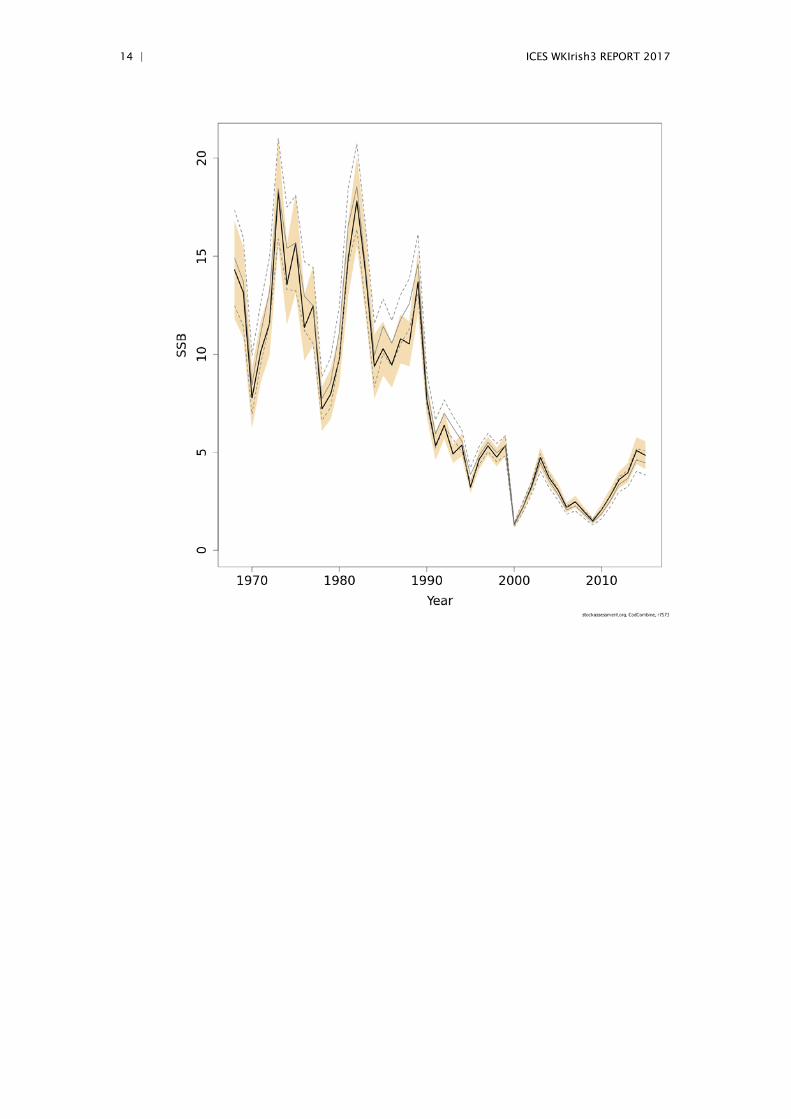
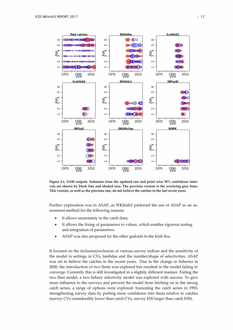
Figure 4.1. SAM outputs. Estimates from the updated run and point wise 95% confidence inter-vals are shown by black line and shaded area. The previous version is the overlying grey lines. This version, as well as the previous one, do not believe the catches in the last seven years.
Further exploration was in ASAP, as WKIrish3 preferred the use of ASAP as an as-sessment method for the following reasons:
• It allows uncertainty in the catch data; • It allows the fixing of parameters to values, which enables rigorous testing
and integration of parameters; • ASAP was also proposed for the other gadoids in the Irish Sea.
It focused on the inclusion/exclusion of various survey indices and the sensitivity of the model to settings in CVs, lambdas and the number/shape of selectivities. ASAP was set to believe the catches in the recent years. Due to the change in fisheries in 2000, the introduction of two fleets was explored but resulted in the model failing to converge. Currently this is still investigated in a slightly different manner. Failing the two fleet model, a two fishery selectivity model was explored with success. To give more influence to the surveys and prevent the model from latching on to the strong catch series, a range of options were explored: truncating the catch series in 1993, strengthening survey data by putting more confidence into them relative to catches (survey CVs considerably lower than catch CVs, survey ESS larger than catch ESS).

18 | ICES WKIrish3 REPORT 2017
The following runs were performed. The model diagnostics are available on the SharePoint under the section working documents (cod_asap_diagnostics - runXX.pdf).
Run 1–Exploratory run
The first run was presented at the workshop after a range of settings and tests prior to the workshop. This was a run including two catch selectivities, catch CVs of 0.2 (1968–2002, 2007–present) /0.8 (2003–2006) and survey CVs as in Run 4. A number of settings were changed during the workshop to provide a more realistic starting point (see run 2).
Run 2-Base run
The settings of the base run were similar for the cod, haddock and whiting ASAP models. They are described below.
Input Justification
Fleets A single fleet (see final run for justification).
Selectivity Three selectivity blocks were used to allow a smooth transition to reflect changes in fishery from 2000 onwards. Additionally the second block was to ensure that older fish would be represented in-between the first selectivity block and the start of the UKFSPW survey. 1st Block (1968–1999): Single logistic 2nd Block (2000–2006): Fixed to 1 for ages 2,3 and 4 3rd Block: Double logistic
Index specification
The two Northern Irish groundfish surveys (Q1 and Q4) were included (Q1: ages 1–4, Q4: ages 0–2), the UKFSPW (ages 2–5) survey as well as the NI MIK net survey (see final run for justification).
Index selectivity
The MIK net only catches one age class (age 0). Q1 Groundfish: set to 1 ages 2–4 and estimated at-age 1 Q4 Groundfish: Estimated for ages 0–2 UKFSPW: Single logistic function
Index CV and ESS
The CVs of the two NI groundfish indices were set to CVs calculated from survey data. The CV for the MIK net was set to 0.7; The CV for the UKFSP was set to 0.4. The effective sample size for the proportions-at-age was set at 50 for all surveys including catch-at-age information which was slightly lower than the number of stations in the survey.
Fleet CV and ESS
The CV for the catches (catch volume) was initially set at 0.05 for all years except 2003–2005. Years 2003–3005 had experienced problems in fisheries data collection which is reflected in CVs of 0.075. The actual precision is lower but the starting point was to assume accurate and precise catch data. The effective samples size for the proportions-at-age was set at 100 prior 1990, 50 from 1990 onwards. Years 2003–2005 were assigned values of 1 to reflect the poor data quality.
Recruitment Deviations
The CV for recruitment deviations was set at 0.5 to allow considerable variability between years, the lambda was set to 0.1 to allow unconstrained variation in recruitment.

ICES WKIrish3 REPORT 2017 | 19
Run 3–M =0.2
M was set to 0.2 for all ages/years as in recent cod assessment. All other parameters were equal to base run.
This change had more impact on the stock trend than any of the other changes. Changes had effect on the stock–recruitment which was considerably lower than in the base run. SSB was lowest of all runs and F highest. Lorenzen M is considered to be a better reflection of mortality and has been applied to other gadoid stocks in Eu-rope.
Run 4–survey CVs
The survey CVs of Q1 were reduced to 0.2 and those of Q4 to 0.4 as in the exploratory runs. This was to investigate the impact of rather high CV settings in the base run which uses real CV values. All other settings like base run. This change had little im-pact on the output, it was hence decided to use real survey CVs.
Run 5–Two selectivities (option 1)
Catch selectivity blocks were reduced to two, removing the third selectivity block. All other settings were as in the base run. Fit-at-age in catch declined slightly, otherwise there was little impact on the model output.
Run 6–Truncate time-series in 1993
Because the model has been observed to latch onto the strong catch curve at an early point in time, it was considered to truncate the catch series prior to 1993.
Though likelihood results are not comparable to those of the other runs, the cut of the catch curve had no impact on the dynamics in the later years.
Run 7–Two selectivities (option 2)
Catch selectivities were reduced to two blocks. In contrast to Run 5 the third block was removed and the second block was allowed to be estimated by a double logistic function. All other settings were like base run. The outcome was a strong dome-shaped selection curve for the second selectivity block.
This run produced the best likelihoods and best fit of catch-at-age and survey at-age data.
This option is the best at the current time, but will have to be revisited should the fishery one day return to a fleet targeting large cod.
Run 8–Less precise catch data
The catch CV was increased to 0.1 (0.15 for year 2003–2005) which was believed to be more realistic. All other settings like base run.
These changes had very little impact on the stock trend but poor fit to catches and surveys.

20 | ICES WKIrish3 REPORT 2017
Comparison of stock trends
Figure 4.2 provides an overview of the runs described above.
Table 4.1. Likelihoods/objective functions for the various runs and parameters. Highlighted are generally the two best fitting runs for each parameter. Run 6 was not comparable due to the na-ture of the run (time-series 1993–2015).
RUN TOTAL CATCH TOTAL
INDEX CATCH
AGE COMP
CATCH-AT-AGE
INDEX
N YEAR 1 RECRUITMENT
DEVIATION
1 2589.65 405.748 631.974 514.234 428.858 52.79 537.212
2 1758.36 303.199 440.806 563.433 392.825 54.72 5.417
3 1705.55 302.866 443.041 517.698 380.019 51.01 4.423
4 1794.68 305.412 468.221 562.56 399.37 55.01 5.463
5 1808.66 303.445 445.694 603.438 398.13 55.16 5.463
6 This run is not comparable in Likelihoods due to a considerably shorter time-series
7 1721.06 303.251 440.851 529.301 381.354 54.69 5.415
8 1785.99 336.971 439.989 561.308 390.927 53.09 5.422
Figure 4.2. Comparing the 8 runs as listed above.

ICES WKIrish3 REPORT 2017 | 21
4.3.2 Final assessment model run
Describe the model configuration and justify the choice of settings
TYPE NAME YEAR RANGE AGE RANGE VARIABLE FROM
YEAR TO YEAR?
Caton Catch in tonnes 1968–current Yes (except years 2003–2005)
Canum Catch-at-age in numbers
1968–current 0–6+ Yes (except years 2003–2005)
Weca Weight-at-age in the commercial catch
1968–current 0–6+ Yes (except years 2003–2005)
West Weight-at-age of the spawning stock at spawning time.
1968–current 0–6+ Yes (except years 2003–2005)
Mprop Proportion of natural mortality before spawning
1968–current 0–6+ No
Fprop Proportion of fishing mortality before spawning
Not relevant
Matprop Proportion mature at-age
1968–current 0–6+ Yes
Natmor Natural mortality 1968–current 0–6+ No
The final run was Run 7, based on the best likelihood fit and most appropriate set-tings. The two-selectivity approach with the dome-shaped 2nd selectivity block is prioritized over the three selectivity base run as a simpler model. The effect on the stock trend was very small. This can probably be explained by the lack of older fish in the population. If the age structure recovers, it might be important to consider the three selectivity option again.

22 | ICES WKIrish3 REPORT 2017
The final settings are justified below.
Input Justification
Fleets A single fleet was used because models with separate landings and discard fleets were unlikely to converge.
Selectivity Two selectivity blocks were used in the final run, with the first selectivity block (1968–1999) an asymptotic shape and the second one a sharply dome-shaped. For cod and haddock, fisheries selectivity is believed to have changed with the decline of the midwater gadoid fleet and introduction of restrictions in 2000. The choice of selectivity blocks was based on patterns in the logratios of the catch numbers-at-age (cnaa) as well as estimated F patterns in runs with a single selectivity block. The final choice for two selectivity blocks rather than three was for a simpler model. It was also based on a better likelihood fit. Allowing the second selectivity block to dome-shape rather than to force it to higher selectivity values for ages 2–4 resulted in a better fit and is likely to represent the current fishery better. If the age structure recovers, it might be important to consider this option again.
Catch All available age classes (age 0–6) were included. Note that ASAP treats the first age class (in this case age 0) as age 1. Therefore the outputs need to be offset by one age class.
Index specification
The two Northern Irish groundfish surveys (Q1, ages 1–4, and Q4, ages 0–2) were included (all available ages) as well as the NI MIK net survey and UK FSPW (ages 2–5) survey.
Index selectivity
The MIK net only catches one age class (age 0). Q1 Groundfish: set to 1 ages 2–4 and estimated at-age 1 Q4 Groundfish: Estimated for ages 0–2 UKFSPW: Single logistic function
Index CV and ESS
The CVs for all years of the two NI groundfish indices were set to real Q1 and Q4 survey CVs. CVs of all years for MIKNET were set to 0.7 and to 0.4 for UKFSPW. The effective sample size for the proportions-at-age was set at 50 which was slightly lower than the number of stations in the survey.
Fleet CV and ESS
The CV for the catches (catch volume) was initially set at 0.05 for all years, except 2003–2005 it was 0.075 to represent difficulties in sampling and high uncertainties in those years. The effective samples size for the proportions-at-age was set at 100 for years 1968–1990 and to 50 for 1991–present to reflect the small number of fish sampled for age from large portions of the catch. Years 2003–2005 were assigned an effective sample size of 1 to account for the absence of sampling effort.
Recruitment deviations
Lambda for recruitment deviations was set at 0.1 to allow unconstrained variation in recruitment. If future runs fail to converge Lambda can be set to 1 with a high CV to reduce the number of parameters. This appears to have very little impact on the stock trend or fit to catches.

ICES WKIrish3 REPORT 2017 | 23
Diagnostic plots
Figure 4.3. Catch Fit.

24 | ICES WKIrish3 REPORT 2017

ICES WKIrish3 REPORT 2017 | 25
Figure 4.4. Catch proportion-at-age residuals, bottom figure Standardized residuals.

26 | ICES WKIrish3 REPORT 2017
Figure 4.5. Index fit.
Figure 4.6. Catch-at-age proportion index fit.

ICES WKIrish3 REPORT 2017 | 27

28 | ICES WKIrish3 REPORT 2017
Figure 4.7. Index proportion-at-age residuals.

ICES WKIrish3 REPORT 2017 | 29
Figure 4.8. Catch selectivities, block 1: 1968–1999, Block 2: 2000–current.
Figure 4.9. Index selectivities: Index1-Q1, index2-Q4, Index3-UKFSPW, Index4-MIKNET.
30 | ICES WKIrish3 REPORT 2017
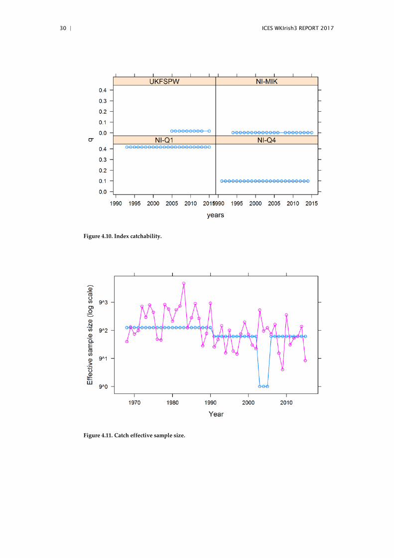
Figure 4.10. Index catchability.
Figure 4.11. Catch effective sample size.

ICES WKIrish3 REPORT 2017 | 31
Figure 4.12. Index effective sample size.
Figure 4.13. Log stock numbers-at-age.

32 | ICES WKIrish3 REPORT 2017
Figure 4.14. Objective function.
Figure 4.15. RMSE fit.
ICES WKIrish3 REPORT 2017 | 33
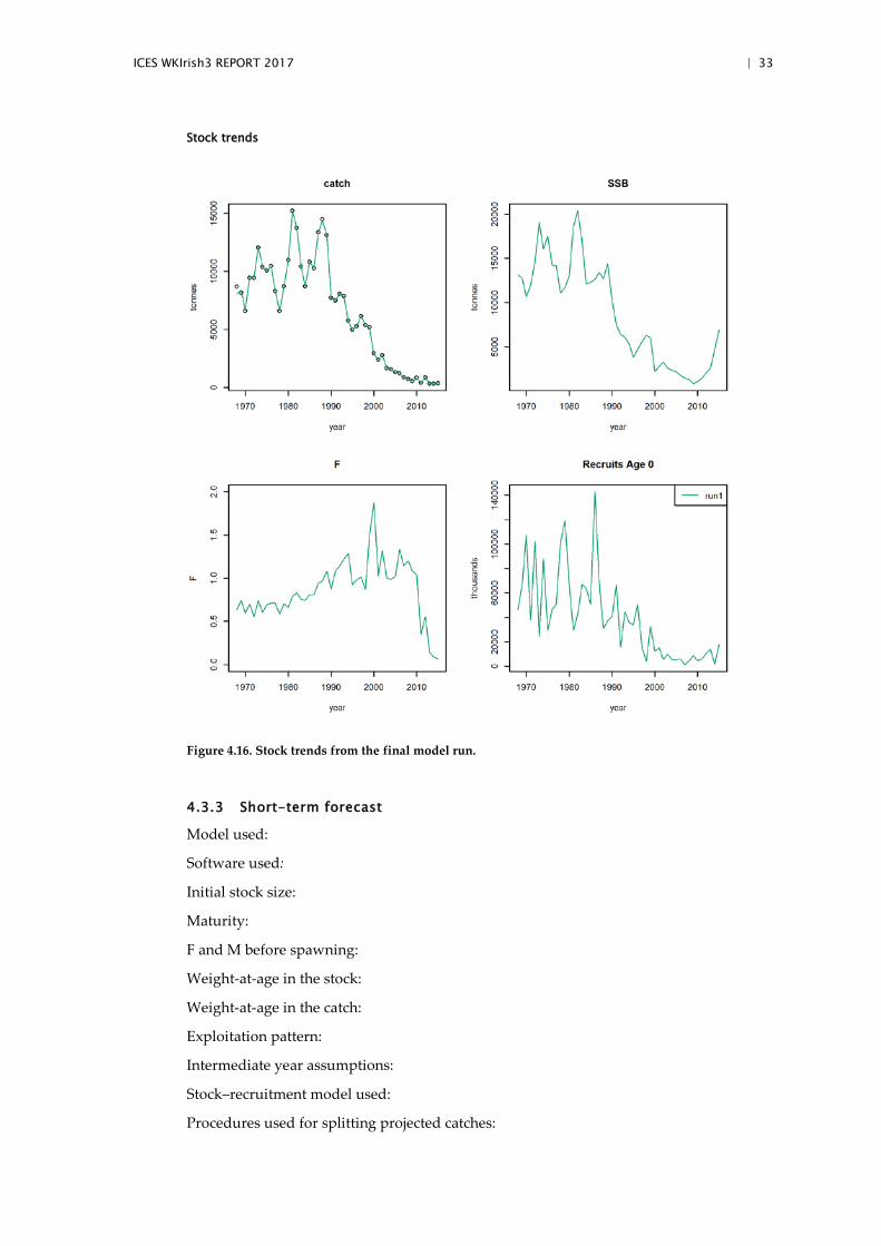
Stock trends
Figure 4.16. Stock trends from the final model run.
4.3.3 Short-term forecast
Model used:
Software used:
Initial stock size:
Maturity:
F and M before spawning:
Weight-at-age in the stock:
Weight-at-age in the catch:
Exploitation pattern:
Intermediate year assumptions:
Stock–recruitment model used:
Procedures used for splitting projected catches:

34 | ICES WKIrish3 REPORT 2017
4.4 Reference points
The derivation of the MSY reference points is described in Annex 8.
TYPE VALUE TECHNICAL BASIS
MSY MSY Btrigger 17 521 t Bpa
Approach FMSY 0.61 Median point estimates of ‘EqSim’ simulations
Blim 6000 t Suggested breakpoint in SSB where recruitment changes
Precautionary Bpa 17 521 t Blim combined with the assessment error; Blim x exp(1.645 x σ); σ = 0.15
Approach Flim 1.27 F with 50% probability of SSB < Blim
Fpa 0.914 Flim combined with the assessment error; Flim x exp(-1.645 x σ); σ = 0.2
4.5 Future research and data requirements
Introduction of multiple fleets
The stock has been harvested by a range of different fleets and vessels/gears. A step forward will be to explore the introduction of multiple fleets to the model which would represent these trends.
4.6 Multispecies information: WKIrish4
None identified.

ICES WKIrish3 REPORT 2017 | 35
5 Irish Sea haddock
Stock assessment models for Irish Sea haddock were explored during WKIrish3. Ex-ploratory assessment models were formulated for the stock on the basis of the issue list below and data decisions made at WKIrish 2. Initial model solutions were com-pared with existing trends based assessment model (SurbaR) and model solutions previously used for the stock (XSA). Potential assessment solutions explored includ-ed SAM, A4A and ASAP and update of SPiCT model. Initial exploratory model con-figurations are presented in working documents provided to WKIrish3.
5.1 Issue list
• Maturity – update to time-series of proportion mature at-age from NIGFS-Q1 by WKIrish2;
• Tuning series – available surveys were reviews updated by WKIrish2; • Discard data incorporated into catch estimates as previously created by
WKRound 2013; • Assessment method – ASAP is proposed as the new assessment method; • Biological reference points – estimated according to ICES procedures.
Not addressed:
• Prey relations – Investigate the role of whiting in Irish Sea multispecies foodweb dynamics;
• Ecosystem drivers – some discussing by WKIrish2, no firm conclusions.
5.2 Data
Data exploration was done by WKIrish2, below is a description of the sensitivity of the proposed model to the input data.
5.2.1 Stock identity and migration
5.2.2 Life-history data
Estimates of natural mortality were calculated at WKIrish2 (ICES, 2016) for a discus-sion on natural mortality, the choice of the Lorenzen method for estimating M is doc-umented in the WKIrish2 report. Assessment runs were performed with M=0.2, Lorenzen M, Lorenzen M rescaled to M=2 at-age 5 and Gislason M. The proportion of fish ‘mature at-age’ was estimated from the NIFGS-Q1 survey for female haddock, with LOWESS smoother fitted for temporal smoothing.
5.2.3 Other biological information
Stock weights-at-age are estimated as the Q1 weights-at-age from survey and com-mercial catches. Stock weights are calculated by fitting a von Bertalanffy growth curve to all available survey estimates of mean length-at-age in March and first-quarter landings, with an additional vector of parameters estimated to allow for year-class effects in asymptotic length.

36 | ICES WKIrish3 REPORT 2017
5.2.4 Fishery-dependent data
An underling requirement of the current assessment exploration is to address chang-es in the quality of the commercial catch series data and assumptions of selectivity change in the fishery due to technical measures and management prescriptions which may have resulted in data quality and fishery selectivity changes over time.
Sensitivity analysis in ASAP model assumptions to the confidence in the catch series was applied by introducing a time-series of variable coefficient of variation (CV) es-timates for the catch estimates. These were formulated to reflect the discussion of the catch estimates presented in WKIrish2 (ICES, 2016).
Sensitivity analysis to fishery selectivity patterns, due to management prescriptions, was explored by means of defining selectivity blocks within the commercial fleet. Blocks were selected to reflect change points in management. The initial model for-mulation consisted of a two block model based on specific time points of manage-ment measures. Sensitivity to introduction of a transitional block to reflect gradual changes in fishery behaviour was explored.
5.2.5 Fishery-independent data
A number of tuning series are available. The suitability of these as input data were explored at WKIrish2 (ICES, 2016). Initial exploration of tuning series identified NIGFS-Q1, NIGFS-Q4, NI-MIK and UKFSPW as robust dataset for inclusion in the assessment models of haddock. Sensitivity testing was applied for scenarios of sur-vey series CV. At WKIRISH2 CV’s for NIGFS-Q1 and NIGFS-Q4 and NIMIK surveys were derived from as observed CVs.
5.2.6 Environmental drivers and ecosystem impacts
Explicit environmental drivers are not included in the current assessment investiga-tion.
5.3 Assessment and forecast
Initial assessment runs were performed using, SurbaR, VPA, XSA, SAM, A4A and ASAP. At present, ASAP is presented as the preferred assessment method for the fol-lowing reasons:
• It allows uncertainty in catch data to be accounted for; • Allows appropriate incorporation of selectivity change; • ASAP was also proposed for the other gadoids in the Irish Sea.
5.3.1 Assessment models and runs
Run 1: Exploratory model
A preferred model ASAP model configuration was presented at the workshop. Re-view of initial model explorations and normalisation with other Irish Sea gadoid spe-cies being explored at WKIrish3 suggested provided a base model configuration as detailed in Table 5.1.
The initial model included three tuning indices, NIGFS-Q1, NIGFS-Q4 & NI-MIK. A highly divergent retrospective pattern when the UKFSPW index was included was reported. The model included two selectivity blocks in fishery-dependent data, re-flecting bycatch and targeted fishery until the year 2000 (asymptotic). This was re-

ICES WKIrish3 REPORT 2017 | 37
placed by a fleet selectivity pattern without targeted fishing of older fish (dome-shaped) after 2000, reflecting management measures.
Table 5.1. Initial model configuration and justification (Base Model).
INPUT JUSTIFICATION
Fleets A single fleet was (see final run for justification).
Selectivity Two selectivity blocks were used. Block 1; 1993 to 2000 asymptotic selection reflecting bycatch and targeted nature of catches. Block 2; 2001 to present domed-shaped selection reflecting limited targeted fishery activity.
Index specification
NIGFS-Q1 [ages 1 : 4]; NIGFS-Q4 [age 0:3]; NIMIK [age 0].
Index selectivity
Selectivity-at-age for NIGFS-Q1 and NIGFS-Q4 surveys were asymptotic.
Index CV and ESS
The CVs for NIGFS-Q1 and NIGFS-Q4 indices were as observed for numbers of fish measured between stations; the effective sample size for the proportions-at-age was set at 50 which is slightly lower than the number of stations in the survey (63).
Fleet CV and ESS
The CV for the catches (catch volume) was initially set at 0.3 <2003, 0.7 for 2003–2006 and 0.3 2007 to present. The effective samples size for the proportions-at-age was set at 50 for all years apart from 2003–2006 when it is set to 1.
Recruitment Deviations
The CV for recruitment deviations was set at 1 to allow considerable variability between years.
Run 2: Normalisation to Irish Sea gadoids
Review of initial model explorations and in discussion with other gadoid stocks be-ing examined at WKIrish3 initial settings were normalised between stocks to reflect the shared fishery history, survey sources and sampling of commercial fisheries. This refined the catch CV to a 0.35 before 2003, 0.4 during 2003–2006 and 0.30 after 2006. Examination of this initial in Run 1 model suggested that it was disproportionally tuned to the survey series compared to the catch series (Figure 5.1). In the Run 2 the CV for survey series was set to 0.3 for NIGFS-Q1 & NIGFS-Q4 and 0.6 for NI-MIK.

38 | ICES WKIrish3 REPORT 2017
Figure 5.1. Fitted and observed index and catch series from model Run 2.
Run 3: Sensitivity to catch coefficient of variation
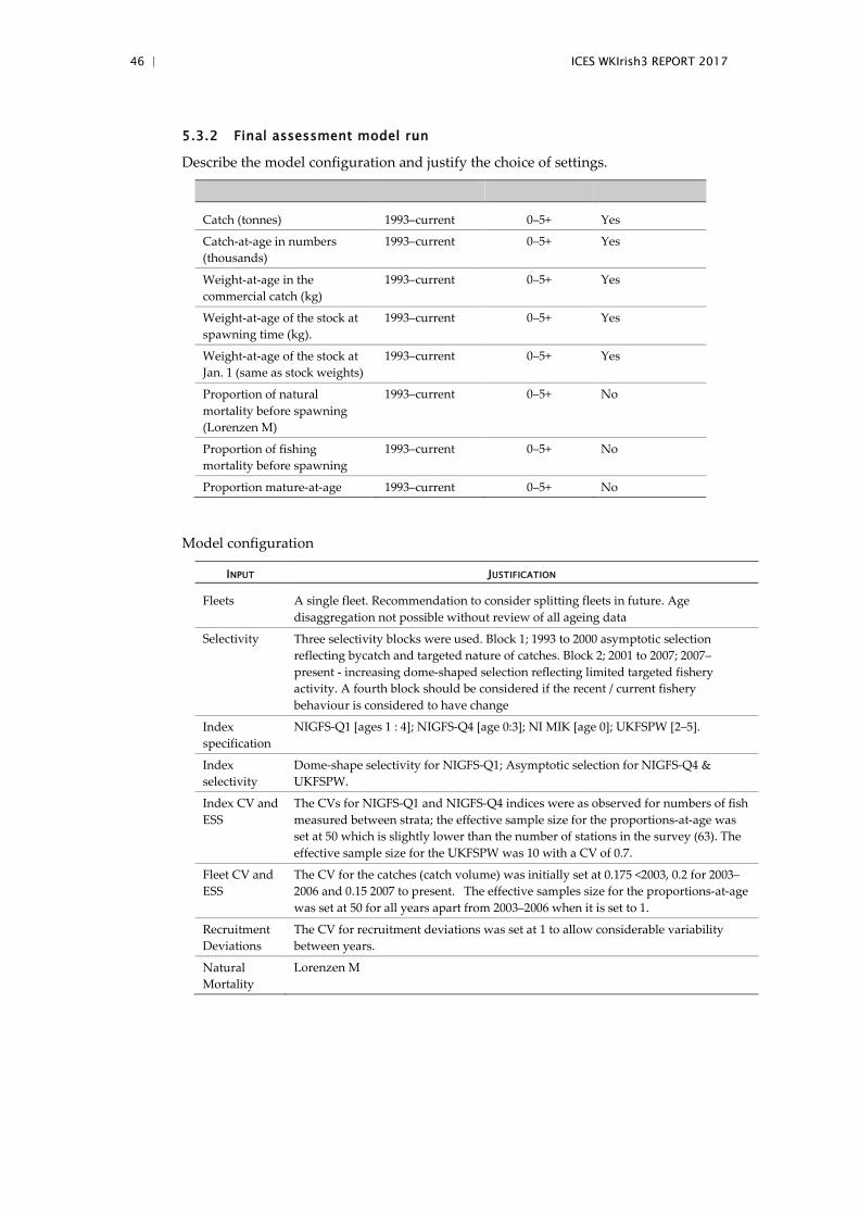
It was proposed that a sensitivity analysis to catch CV scenarios was required with fixed CVs of survey series. The catch information from 2007 to present is regarded as the most confident, during 2003–2006 it is regarded that catch and sampling infor-mation is of relatively lower quality due to lack of sampling opportunity. Before 2003 the catch series is regarded as of intermediate confidence. The highest confidence pe-riod was initially set at 0.05, 0.1 and 0.075, for the high, low and intermediate confi-dence periods. These CVs were increased by increments of 0.025 for 5 iterations and settings as in Run 1. The model fit and log-likelihood compared (Figures 5.2 and 5.3 and Table 5.2).
Examination of the model fit log-likelihoods shows that selecting highest confidence in catch resulted in the smallest overall log-likelihood, but demonstrated that this was a trade-off between fit to the indices vs. fit the catch. There was clear incremental improved of fit to catch by increasing the confidence scenario (Figure 5.2). However, the highest catch confidence resulted in a fit to the survey indices which were sub-stantially different from that achieved by other scenarios. The survey indices are re-garded to reflect the stock status and track clear classes well (WKIrish2), furthermore data issues have been noted with catch data, including back population of a discard series and low confidence associated with applying mist report estimates before 2007.
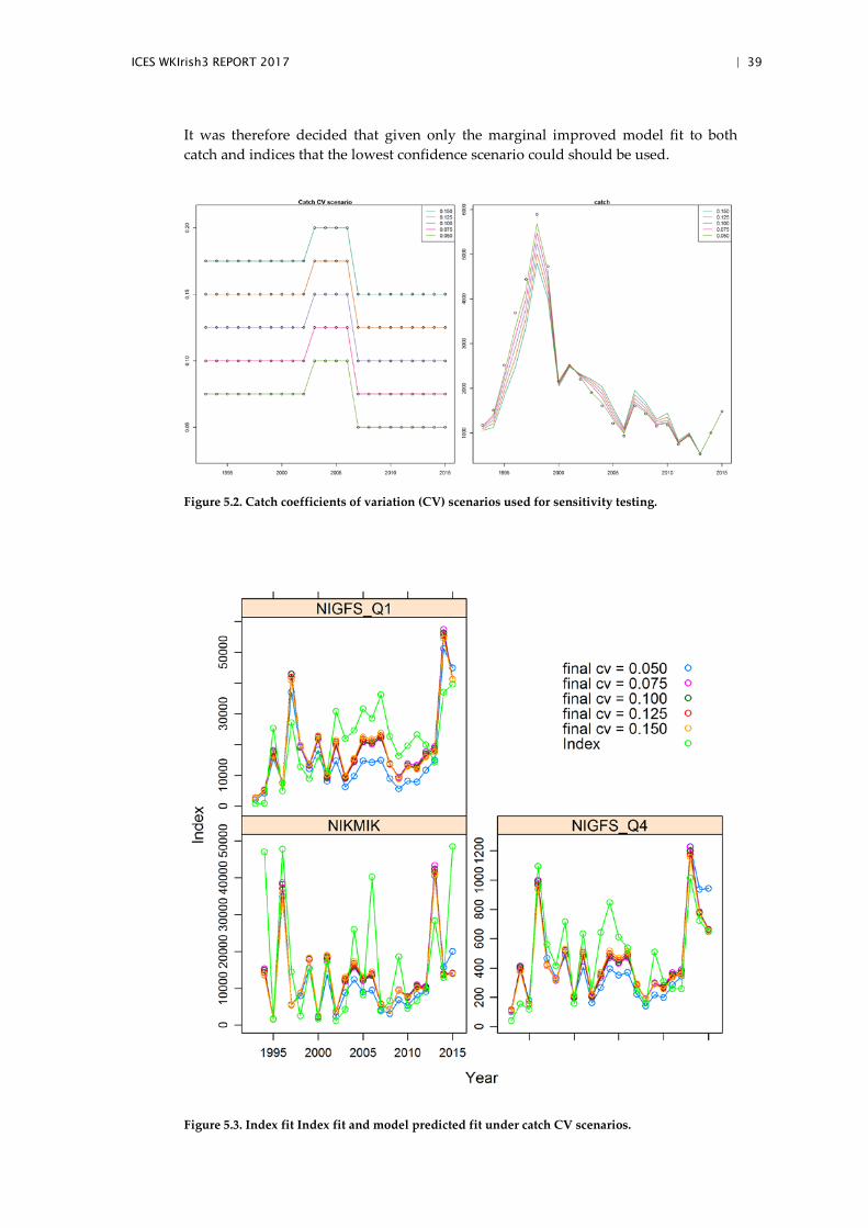
ICES WKIrish3 REPORT 2017 | 39
It was therefore decided that given only the marginal improved model fit to both catch and indices that the lowest confidence scenario could should be used.
Figure 5.2. Catch coefficients of variation (CV) scenarios used for sensitivity testing.
Figure 5.3. Index fit Index fit and model predicted fit under catch CV scenarios.

40 | ICES WKIrish3 REPORT 2017
Table 5.2. Model fit log likelihood values for catch coefficient of variation (CV) sensitivity test-ing.
CATCH CV TOTAL CATCH INDEX CATCH AGE INDEX AGE SELECTIVITY PARAMETERS INDEX SELECTIVITY
0.15* 1370.96 164.53 639.21 204.44 347.42 14.87 0.49
0.125 1371.15 158.46 642.35 205.43 350.39 14.10 0.43
0.1 1370.33 151.20 644.93 206.47 354.23 13.15 0.35
0.075 1367.89 142.74 646.33 207.54 358.93 12.08 0.27
0.05 1336.14 133.07 663.16 192.03 337.70 9.48 0.71
*Selected model for further sensitivity testing and model configuration runs.
Run 4: Sensitivity to natural mortality assumptions
At WKIrish2, Lorenzen estimates of M and Gislason estimates of M were calculated for Irish Sea haddock. Sensitivity to these estimates was carried out using the model selected from Run 3. In addition to Lorenzen and Gislason estimates, a rescaled Lo-renzen M was used, with M = 0.2 at oldest age (5) and M=0.2, for all ages (Figure 5.4).
Examination of the model fit log-likelihoods supported selection of the Lorenzen es-timates of natural mortality, with the lowest total log-likelihood of all sensitivity, and lowest log-likelihood to catch age survey age (Table 5.3). The Lorenzen M estimates were selected for further sensitivity testing and model configuration runs.
Figure 5.4. Estimates of natural mortality used for sensitivity testing.

ICES WKIrish3 REPORT 2017 | 41
Table 5.3. Model fit log-likelihood values for natural mortality sensitivity testing.
NATURAL MORTALITY TOTAL CATCH INDEX CATCH AGE INDEX AGE SELECTIVITY PARAMETERS INDEX SELECTIVITY
Lorenzen* 1370.96 164.53 639.21 204.44 347.42 14.87 0.49
M=0.2 1560.86 158.05 634.45 299.42 462.36 1.83 4.74
Re-scaled Lorenzen 1398.63 163.05 636.78 215.83 369.65 7.80 5.53
Gislason 2382.95 151.31 637.43 734.76 452.45 404.57 2.43
*Selected model for further sensitivity testing and model configuration runs.
Run 5: Sensitivity to survey CV assumptions
At WKIrish2 coefficients of variation were calculated for survey indices, as CV of the number of fish measured between survey strata. These observed CVs were used and comparison made with a fixed CV, as used in Run1 and a rescaled observed CV, re-scaled to have a mean of the fixed CV. A lower limit of 0.1 was applied to all ob-served CVs.
The CV series for indices and the resultant fit of the model to observer catch is shown in Figure 5.5. Examination of the log-likelihood values of the model fit (Table 5.4). Using observed CVs resulted in the best model fit in terms, of total fit, fit to catch se-ries, fit to survey series, fit to catch age and fit to index age. Using an observed CV series was selected for further model configuration runs and sensitivity testing.
Table 5.4. Model fit log likelihood values for natural mortality sensitivity testing.
SURVEY CV TOTAL CATCH INDEX CATCH AGE INDEX AGE SELECTIVITY PARAMETERS INDEX SELECTIVITY
Fixed 1370.96 164.53 639.21 204.44 347.42 14.87 0.49
Scaled 1374.12 167.62 643.73 202.49 343.74 16.03 0.52
Observed* 1359.44 160.57 640.27 200.85 340.79 16.40 0.56
*Selected model for further sensitivity testing and model configuration runs.

42 | ICES WKIrish3 REPORT 2017
Figure 5.5. Time-series of indices coefficient of variation (CV) used in sensitivity testing and model fit to catch series.
Run 6: Sensitivity to Survey selectivity
Initial model configuration and testing was applied with asymptotic selection by age for survey series. It was discussed during the benchmark meeting that it is likely that the survey gear used in the NIGFS-Q1 and Q4 surveys is likely to have a domed-shaped selectivity. Domed shape selectivity was parameterised using the double lo-gistic function for the NIGFS-Q1 survey. Given the age range used in the NIGSF-Q4 survey the selectivity pattern was retained as asymptotic.
Although considered a more appropriate selection pattern for the NIGFS-Q1 survey dome shaped selection did not provide an overall improved (Table 5.5). It was con-

ICES WKIrish3 REPORT 2017 | 43
sidered necessary to examine this assumption in the context of the imposed break-point in catch selectivity and the inclusion of a tuning series which targeted old fish, namely the UKFSPW series.
Table 5.5. Model fit log likelihood values for assumptions of selectivity of NIGFS-Q1 survey.
SURVEY SELECTIVITY TOTAL CATCH INDEX CATCH AGE INDEX AGE SELECTIVITY PARAMETERS INDEX SELECTIVITY
Domed* 1373.63 159.59 649.46 200.87 349.07 11.27 3.39
Asymptotic 1359.44 160.57 640.27 200.85 340.79 16.40 0.56
*Selected model for further sensitivity testing and model configuration runs.
Figure 5.6. NIGFS index selectivity scenarios tested and stock trend plots of model fit to catch, predicted SSB, recruitment and fishing pressure – F.
Run 7: Sensitivity to catch selectivity
In the previously model configurations a breakpoint in selectivity was applied in 2000, associated with management measures to reduce fishing mortality on cod. A third selectivity block was suggested to allow a transition between a fully selected stock to a regime without targeted fishing of older fish. A third selectivity was intro-duced form 2000–2007. The initial block prior to 2000 was maintained as a asymptot-ic, with the later blocks fitted as age-based selection using defined coefficients of selectivity for each age; allowing the model to select final parameterisation, but giv-ing initial values which reflected an increasingly dome shape selection in the later two blocks. The log-likelihood model fit parameters in Table 5.6 support the use of a three selectivity blocks. This configuration was selected for trial with the inclusion of the UKFSPW index.

44 | ICES WKIrish3 REPORT 2017
Figure 5.7. Selectivity patterns applied for a two block and three block selectivity pattern for the fishery.
Table 5.6. Model fit log-likelihood values comparison for a two block and three block fishery selectivity model.
FISHERY SELECTIVITY TOTAL CATCH INDEX CATCH AGE INDEX AGE SELECTIVITY PARAMETERS INDEX SELECTIVITY
Two Blocks 1373.634 159.5875 649.4597 200.8671 349.0659 11.26902 3.385016
Three Blocks* 1344.325 159.2254 641.9206 201.5052 338.3684 -0.68547 3.991138
*Selected model for further comparison with model including UKFSPW survey.
Run 8: Sensitivity to inclusion of UKFSPW survey
Having both a dome-shape selection in the fishery, NIGFS-Q1 survey prompted a requirement to include a source of information for older aged fish, with higher selec-tivity coefficients. The UKFSPW survey a continuing survey series, targeting older fish was included, although the series is short; 2007–present (excluding 2014). While the log-likelihood fit of the model including a fourth index was not reduced, the ad-ditional information provided by the index was deemed an important addition. The UKFSPW index includes the only fully selected source of information for the oldest age fish. It is assumed to asymptotic selection of fish, in contrast to the NIGFS-Q1 and NIGFS-Q4 surveys which target juvenile fish and commercial fishery data which, due to recent management measures has resulted in limited targeted fishing form had-dock.
The use of current specified selectivity blocks may require review at annual at regular intervals. With advice and management for haddock or other species it is possible that the character of the fishery may change. A model including the UKFSPW survey with four selectivity blocks was applied (Table 5.7). In recent years 2013–present it has been observed that targeted fishing of haddock has increased, due to the strength of the 2013 year class. As this year class has matured and the cohort progressed full

ICES WKIrish3 REPORT 2017 | 45
selection of the older fish may need to be taken into consideration in model configu-ration; at present this selectivity period is too short to be parameterised robustly.
Table 5.7. Model fit log-likelihood values comparison of models including the FSP index and a model with this index.
FOURTH INDEX TOTAL CATCH INDEX CATCH AGE INDEX AGE SELECTIVITY PARAMETERS INDEX SELECTIVITY
UKFSPW excluded 1344.325 159.2254 641.9206 201.5052 338.3684 -0.68547 3.991138
UKFSPW* included 1426.381 158.809 677.7911 200.102 382.1372 0.311632 7.229801
4 Block model 1458.015 163.691 681.8343 196.782 409.185 -1.098711 7.621659
*Final model configuration.
A retrospective analysis demonstrated a consistent historic downward revision of the perceived SSB trend and upward revision of the F trend. The initial two years of the retrospective plot show significant deviations. This was considered due to the model having a selectivity block, beginning in 2007, with reduced selection for older fish and the introduction of the UKFSPW, with an asymptotic selectivity pattern, starting in 2007. The short period to estimate the selectivity parameters for both the fishery and survey index are considered to contribute to the instability of the model during this time.
Figure 5.8. A retrospective plot the final assessment model.
46 | ICES WKIrish3 REPORT 2017
5.3.2 Final assessment model run
Describe the model configuration and justify the choice of settings.
Catch (tonnes) 1993–current 0–5+ Yes
Catch-at-age in numbers (thousands)
1993–current 0–5+ Yes
Weight-at-age in the commercial catch (kg)
1993–current 0–5+ Yes
Weight-at-age of the stock at spawning time (kg).
1993–current 0–5+ Yes
Weight-at-age of the stock at Jan. 1 (same as stock weights)
1993–current 0–5+ Yes
Proportion of natural mortality before spawning (Lorenzen M)
1993–current 0–5+ No
Proportion of fishing mortality before spawning
1993–current 0–5+ No
Proportion mature-at-age 1993–current 0–5+ No
Model configuration
INPUT JUSTIFICATION
Fleets A single fleet. Recommendation to consider splitting fleets in future. Age disaggregation not possible without review of all ageing data
Selectivity Three selectivity blocks were used. Block 1; 1993 to 2000 asymptotic selection reflecting bycatch and targeted nature of catches. Block 2; 2001 to 2007; 2007–present - increasing dome-shaped selection reflecting limited targeted fishery activity. A fourth block should be considered if the recent / current fishery behaviour is considered to have change
Index specification
NIGFS-Q1 [ages 1 : 4]; NIGFS-Q4 [age 0:3]; NI MIK [age 0]; UKFSPW [2–5].
Index selectivity
Dome-shape selectivity for NIGFS-Q1; Asymptotic selection for NIGFS-Q4 & UKFSPW.
Index CV and ESS
The CVs for NIGFS-Q1 and NIGFS-Q4 indices were as observed for numbers of fish measured between strata; the effective sample size for the proportions-at-age was set at 50 which is slightly lower than the number of stations in the survey (63). The effective sample size for the UKFSPW was 10 with a CV of 0.7.
Fleet CV and ESS
The CV for the catches (catch volume) was initially set at 0.175 <2003, 0.2 for 2003–2006 and 0.15 2007 to present. The effective samples size for the proportions-at-age was set at 50 for all years apart from 2003–2006 when it is set to 1.
Recruitment Deviations
The CV for recruitment deviations was set at 1 to allow considerable variability between years.
Natural Mortality
Lorenzen M

ICES WKIrish3 REPORT 2017 | 47
ASAP model settings
OPTION SETTING
Use likelihood constant Yes
Mean F (Fbar) age range 2–4
Fleet selectivity block 1 Assymtotpic
Fleet selectivity block 2 Age coefficineits (age 0–5) (0.2;0.5;0.8;1;0.7;0.5)
Fleet selectivity block 3 Age coefficients (age 0–5) (0.3;0.6;0.7;8;0.6;0.4)
Discards Included in catch (not specified separately from landings)
Index units 4 (numbers)
Index month NIGFS-Q1 (3); NIGFS-Q4 (10); NIMIK (7); UKFSPW(3)
Index selectivity linked to fleet -1 (not linked)
Index age range NIGFS-Q1 (1–4); NIGFS-Q4 (0–3); NIMIK (0); UKFSPW(2–5)
Index Selectivity (NIGFS-Q1) Double logistic
Index Selectivity (NIGFS-Q4) Asytotpic
Index Selectivity (NIMIK) NA (age 0 only)
Index Selectivity (UK-FSPW) Aysmytotic
Index CV & ESS (NIGFS-Q1) Observed strata CV (lower limit 0.1); ESS = 50
Index CV & ESS (NIGFS-Q4) Observed strata CV (lower limit 0.1); ESS = 50
Index CV & ESS (NIMIK) Observed station CV (lower limit 0.1); ESS = 50
Index CV & ESS (UK-FSPW) CV = 0.7; ESS = 10
Phase for F-Mult in 1st year 1
Phase for F-Mult deviations 2
Phase for recruitment deviations 3
Phase for N in 1st Year 1
Phase for catchability in 1st Year 3
Phase for catchability deviations -5 (Assume constant catchability in indices)
Phase for unexploited stock size 1
Phase for steepness -5 (Do not fit stock–recruitment curve)
Catch total CV 1993-2000 (0.175); 2003-2006 (0.2); 2007-2015 (0.15)
Catch effective sample size 1993-2000 (50); 2003-2006 (1); 2007-2015 (50)
Lambda for recruit deviations 0 (freely estimated)
Lambda for total catch 1
Lambda for total discards NA (discards included in catch)
Lambda for F-Mult in 1st year 0 (freely estimated)
Lambda for F-Mult deviations 0 (freely estimated)
Lambda for index 1 for both indices in the model
Lambda for index catchability 0 for all indices (freely estimated)
Lambda for catchability devs NA (phase is negative)
Lambda N in 1st year deviations 0 (freely estimated)
Lambda devs initial steepness 0 (freely estimated)
Lambda devs unexpl stock size 0 (freely estimated)

48 | ICES WKIrish3 REPORT 2017
5.3.3 Short-term forecast
Software used: FLAssess – Short-Term Forecast (stf)
Initial stock size Long-term GM (omitting last two years)
Stock numbers-at-age 1 and older from model
Natural mortality Lorenzen M, as in model
Maturity Most rectent estimate
F and M before spawning 0 for all ages in all years
Stock / catch weights-at-age Average last 3 years
Exploitation pattern Average last 3 years
Intermediate year assumptions F in the last year – check retrospective pattern for evidence of bias
Stock–recruit model None, long-term GM recruitment (omitting last two years)
Fbar range 2–4
Rescale to last year No
5.4 Reference points
The derivation of reference points is documented in Annex 9.
Blim was set to the SSB in 1993, from which the fishery developed, an SSB of 2300 t in 1993. The S–R plot for Irish Sea haddock shows no obvious S–R relationship (Figure 5.9), mainly because the recruitment is highly variable. The S–R pairs from 1993:2012 were not used initially as the 2013 recruitment event and 2015 SSB were considered to be highly influential. The fitted relationship, compared to the selecting Blim at 2300 t provides a Blim of 4035 t, a value which has only been exceeded on eight occasions. However, the fitted segmented regression in a much better fitted given an Akaike Information Criterion weight of 94%. Whereas the selected Blim of 2300 t is used pro-posed as a more realistic value for the stock, the modelled relationship is used for further MSY simulations.
The entire time-series is used for MSY simulations (1993–2105). Fcv is 0.22 (F error in last year) and SSBcv as 0.15 (SSB error in last year). Bpa was calculated as Blim com-bined with the assessment error; Blim x exp(1.645 x σ); σ = 0.15 as 3093 t. MSYBtrigger is set to Bpa as the stock has not been fished at or below FMSY for more than five years. FMSY median point estimates is 0.27 (0.273). The upper bound of the FMSY range giving at least 95% of the maximum yield was estimated to 0.35(0.351) and the lower bound at 0.19 (0.192) (Figure 5.4.2). Fp.05, without assessment error of Btrigger as estimated 0.40 (0.0445) and therefore the upper bound does not need to be restricted because of pre-cautionary limits. Flim is estimated to be 0.47 (0.445) as F with 50% probability of SSB <Blim with Fpa as 0.34 calculated as Flim combined with the assessment error; Flim x exp(-1.645 x σ); σ = 0.22.

ICES WKIrish3 REPORT 2017 | 49
Figure 5.9. Stock–recruitment relationship for Irish Sea haddock with fitted segmented regres-sion.

50 | ICES WKIrish3 REPORT 2017
No MYSBtrigger, No error – to estimate Flim.
TYPE VALUE TECHNICAL BASIS
MSY MSY Btrigger 3093 t Bpa
Approach FMSY 0.27 Median point estimates of ‘EqSim’ simulations
Blim 2300t SSB in 1993 – SSB at start of current period of stock development
Precautionary Bpa 3093t Blim combined with the assessment error; Blim x exp(1.645 x σ); σ = 0.15
Approach Flim 0.47 F with 50% probability of SSB <Blim
Fpa 0.34 Flim combined with the assessment error; Flim x exp(-1.645 x σ); σ = 0.22
5.5 Future research and data requirements
This section addresses Tor d)
Consider selection blocks = additional blocks as fishery develops / changes
Consider splitting model
5.6 Multispecies information: WKIrish4
This section addresses Tor e).
Identify aspects that require special attention by the ongoing Irish Sea regional benchmark process, in particular pertaining to the development of integrated multi-species and ecosystem advice (to culminate in the synthesis workshop WKIrish4).

ICES WKIrish3 REPORT 2017 | 51
6 Irish Sea whiting
6.1 Issue list
• Natural mortality – Lorenzen M is proposed to replace 0.2 for all ages • Tuning series – Available surveys were reviewed by WKIrish2 • Discard data reconstruction – Documented by WKIrish2 • Changes in growth and maturity – Documented by WKIrish2 • Assessment method – ASAP is proposed as the new assessment method • Biological reference points – estimated according to ICES procedures
Not addressed:
• Prey relations – Investigate the role of whiting in Irish Sea multispecies foodweb dynamics.
• Ecosystem drivers – some discussing by WKIrish2, no firm conclusions.
6.2 Data
Data exploration was done by WKIrish2, below is a description of the sensitivity of the proposed model to the input data.
6.2.1 Stock identity and migration
See WKIrish2.
6.2.2 Life-history data
See Section 2 for a discussion on natural mortality; the choice of the Lorenzen method for estimating M is documented in the WKIrish2 report. Assessment runs were per-formed with M=0.2 and time-varying M. However there is too much uncertainty about M to justify estimating it for each year as this can potentially just add noise.
Sensitivity to maturity was not investigated; this appears to be consistently knife-edged at-age 2.
6.2.3 Other biological information
6.2.4 Fishery-dependent data
No sensitivity analysis was performed to the fisheries-dependent data.
6.2.5 Fishery-independent data
The inclusion of different available surveys was tested in a series of preliminary model runs. (Described in working document: “WD Whg7a ASAP runs.docx” on the WKIrish3 SharePoint site.)

52 | ICES WKIrish3 REPORT 2017
6.2.6 Environmental drivers and ecosystem impacts
6.3 Assessment and forecast
6.3.1 Assessment models and runs
Exploratory assessment runs were performed using XSA and ASAP (see working documents). WKIrish3 preferred the use of ASAP as an assessment method for the following reasons:
• It allows uncertainty in the catch data; • ASAP is more transparent than XSA; • ASAP was also proposed for the other gadoids in the Irish Sea; • The XSA shows strong trends in catchability residuals and a substantial
retrospective bias.
XSA did inform the periods chosen for selection blocks for the ASAP.
The following runs were performed. The model diagnostics are available on the SharePoint under the section working documents (5_asap_diagnostics - runXX.pdf)
Run 1–Exploratory run
The first run was presented at the workshop. A number of settings were changed during the workshop to provide a more realistic starting point (see run 2).
Run 2–Base run
The settings of the base run were similar for the cod, haddock and whiting ASAP models. They are described below.
Input Justification
Fleets A single fleet was (see final run for justification).
Selectivity Two selectivity blocks were used (see final run for justification).
Index specification
The two Northern Irish groundfish surveys (Q1 and Q4) were included (all available ages) as well as the NI MIK net survey (see final run for justification).
Index selectivity
Selectivity-at-age for the two NI groundfish surveys was set at 1 for all ages (see final run for justification). The MIK net only catches one age class (age 0).
Index CV and ESS
The CVs for all years of the two NI groundfish indices were set to 0.2 (which is similar to the between-station variability of the survey). The CV for the MIK net was set to 0.5; the effective sample size for the proportions-at-age was set at 50 which was slightly lower than the number of stations in the survey.
Fleet CV and ESS
The CV for the catches (catch volume) was initially set at 0.05 for all years. The actual precision is lower but the starting point was to assume accurate and precise catch data. The effective samples size for the proportions-at-age was set at 50.
Recruitment Deviations
The CV for recruitment deviations was set at 1 to allow considerable variability between years. However, the lambda was set to 1, which constrains the recruitment somewhat and helps with convergence.

ICES WKIrish3 REPORT 2017 | 53
Run 3–Less precise catch data
The catch CV was increased to 0.2 which was believed to be more realistic, the effec-tive sample size was reduced to 10 to reflect the small number of age samples taken for significant portions of the catches throughout the time-series. All other settings like run 2.
These changes had very little impact on the stock trend or fit to catches.
Run 4–survey selectivity
The selectivity of the surveys was initially set to 1 for all ages. To investigate if this was a realistic assumption, a single logistic curve was estimated for both groundfish surveys (the MIK net survey only has a single age class). All other settings like run 3.
The logistic curves suggested partial selection for age 1 (and age 0 for the Q4 survey) and full selection for the other ages.
These changes resulted in a slight decrease in SSB in recent years and increase in F but very similar trends. The residual patterns improved somewhat and therefore this change was considered sensible.
Run 5–survey CV
The survey CV was increased to 0.5 to account for additional variability like year-effects. This increase was later considered too high but subsequent runs used this value. All other settings like run 4.
Run 6–time-varying M
Because there have been significant changes in the mean size-at-age, this is likely to affect the natural mortality. A time-varying M was calculated based in the Lorenzen method applied to the catch weights smoothed over five years. All other settings like run 5.
This change had more impact on the stock trend than any of the other changes. In principle this is a sensible approach. However, there is a lack of knowledge of M to justify this approach as it potentially introduces additional noise to the assessment.
Run 7–double logistic survey selectivity
Survey selectivity was estimated by a double logistic curve for both groundfish sur-veys. All other settings like run 5.
The outcome was a strong dome-shaped selection curve for both surveys. However the effect on the stock trend was very small. This can probably be explained by the lack of older fish in the population. If the age structure recovers, it might be im-portant to consider this option again. However because there is very little infor-mation to inform the shape of the curve, therefore the workshop decided to use the simpler single logistic model.
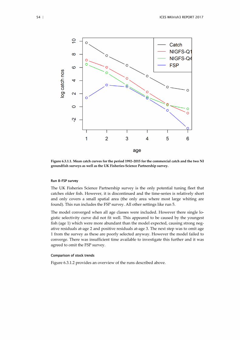
In order to further investigate the possible shape of the selectivity of the surveys, rela-tive to the catches, the mean catch curves over the period of the surveys were plotted (Figure 6.3.1.1). These catch curves were close to parallel, therefore there is no strong evidence of dome-shaped selectivity in the surveys (relative to the commercial catch-es).
54 | ICES WKIrish3 REPORT 2017
Figure 6.3.1.1. Mean catch curves for the period 1992–2015 for the commercial catch and the two NI groundfish surveys as well as the UK Fisheries-Science Partnership survey.
Run 8–FSP survey
The UK Fisheries Science Partnership survey is the only potential tuning fleet that catches older fish. However, it is discontinued and the time-series is relatively short and only covers a small spatial area (the only area where most large whiting are found). This run includes the FSP survey. All other settings like run 5.
The model converged when all age classes were included. However there single lo-gistic selectivity curve did not fit well. This appeared to be caused by the youngest fish (age 1) which were more abundant than the model expected, causing strong neg-ative residuals at-age 2 and positive residuals at-age 3. The next step was to omit age 1 from the survey as these are poorly selected anyway. However the model failed to converge. There was insufficient time available to investigate this further and it was agreed to omit the FSP survey.
Comparison of stock trends
Figure 6.3.1.2 provides an overview of the runs described above.

ICES WKIrish3 REPORT 2017 | 55
Figure 6.3.1.2. Comparison of the stock trends in the exploratory runs. The plots were ‘cropped’ to the last 20 years as the differences between the runs were nearly imperceptible if the full time-series was shown. 1) Exploratory run; 2) Base run; 3) Less precise catch data; 4) survey selectivity; 5) survey CV; 6) time-varying M; 7) double logistic survey selectivity. 8) FSP survey.
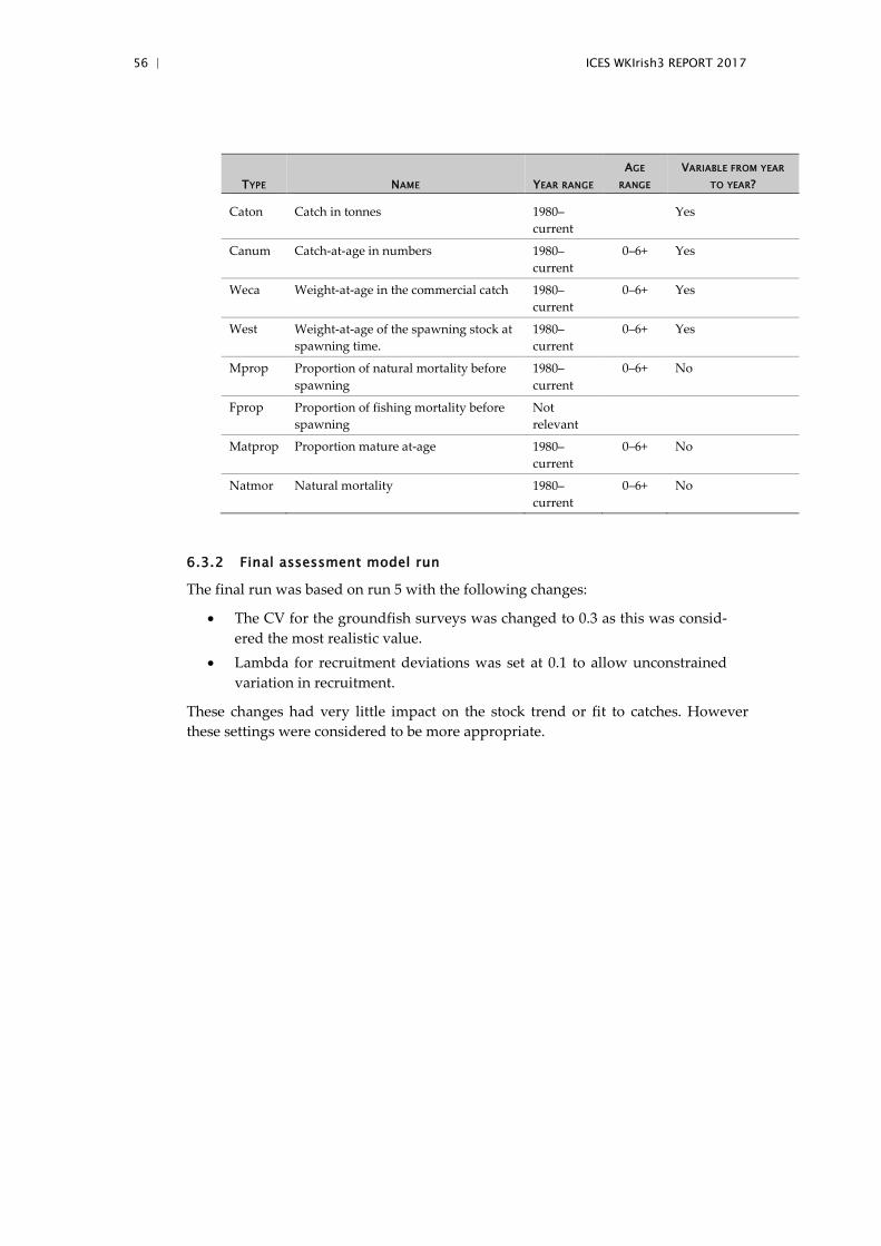
56 | ICES WKIrish3 REPORT 2017
6.3.2 Final assessment model run
The final run was based on run 5 with the following changes:
• The CV for the groundfish surveys was changed to 0.3 as this was consid-ered the most realistic value.
• Lambda for recruitment deviations was set at 0.1 to allow unconstrained variation in recruitment.
These changes had very little impact on the stock trend or fit to catches. However these settings were considered to be more appropriate.
TYPE NAME YEAR RANGE AGE
RANGE VARIABLE FROM YEAR
TO YEAR?
Caton Catch in tonnes 1980–current
Yes
Canum Catch-at-age in numbers 1980–current
0–6+ Yes
Weca Weight-at-age in the commercial catch 1980–current
0–6+ Yes
West Weight-at-age of the spawning stock at spawning time.
1980–current
0–6+ Yes
Mprop Proportion of natural mortality before spawning
1980–current
0–6+ No
Fprop Proportion of fishing mortality before spawning
Not relevant
Matprop Proportion mature at-age 1980–current
0–6+ No
Natmor Natural mortality 1980–current
0–6+ No
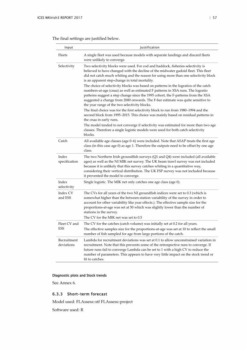
ICES WKIrish3 REPORT 2017 | 57
The final settings are justified below.
Input Justification
Fleets A single fleet was used because models with separate landings and discard fleets were unlikely to converge.
Selectivity Two selectivity blocks were used. For cod and haddock, fisheries selectivity is believed to have changed with the decline of the midwater gadoid fleet. This fleet did not catch much whiting and the reason for using more than one selectivity block is an apparent step-change in total mortality. The choice of selectivity blocks was based on patterns in the logratios of the catch numbers-at-age (cnaa) as well as estimated F patterns in XSA runs. The logratio patterns suggest a step change since the 1995 cohort, the F-patterns from the XSA suggested a change from 2000 onwards. The F-bar estimate was quite sensitive to the year range of the two selectivity blocks. The final choice was for the first selectivity block to run from 1980–1994 and the second block from 1995–2015. This choice was mainly based on residual patterns in the cnaa in early runs. The model tended to not converge if selectivity was estimated for more than two age classes. Therefore a single logistic models were used for both catch selectivity blocks.
Catch All available age classes (age 0–6) were included. Note that ASAP treats the first age class (in this case age 0) as age 1. Therefore the outputs need to be offset by one age class.
Index specification
The two Northern Irish groundfish surveys (Q1 and Q4) were included (all available ages) as well as the NI MIK net survey. The UK beam trawl survey was not included because it is unlikely that this survey catches whiting in a quantitative way, considering their vertical distribution. The UK FSP survey was not included because it prevented the model to converge.
Index selectivity
Single logistic. The MIK net only catches one age class (age 0).
Index CV and ESS
The CVs for all years of the two NI groundfish indices were set to 0.3 (which is somewhat higher than the between-station variability of the survey in order to account for other variability like year effects.). The effective sample size for the proportions-at-age was set at 50 which was slightly lower than the number of stations in the survey. The CV for the MIK net was set to 0.5
Fleet CV and ESS
The CV for the catches (catch volume) was initially set at 0.2 for all years. The effective samples size for the proportions-at-age was set at 10 to reflect the small number of fish sampled for age from large portions of the catch.
Recruitment deviations
Lambda for recruitment deviations was set at 0.1 to allow unconstrained variation in recruitment. Note that this prevents some of the retrospective runs to converge. If future runs fail to converge Lambda can be set to 1 with a high CV to reduce the number of parameters. This appears to have very little impact on the stock trend or fit to catches.
Diagnostic plots and Stock trends
See Annex 6.
6.3.3 Short-term forecast
Model used: FLAssess::stf FLAssess::project
Software used: R

58 | ICES WKIrish3 REPORT 2017
wts.nyears: 3 (Number of years over which to calculate mean for *.wt, *.spwn, mat and m slots)
fbar.nyrs: 3 (Number of years over which to calculate mean for harvest slot)
Intermediate year assumptions: recruitment = GM from 2000 onwards, excluding last year
Stock–recruitment model used: none
Procedures used for splitting projected catches: average proportions landings.n and discards.n last three years
6.4 Reference points
A full re-evaluation of reference points was carried out following the ICES Guidelines (ICES, 2016). This analysis is detailed in Annex 7 and the resulting reference points are provided below.
Whiting in Division 7.a. Reference points, values, and their technical basis.
REFERENCE
POINT VALUE TECHNICAL BASIS
MSY Btrigger 16 300 t Bpa
FMSY 0.22 Median point estimates of EqSim with a combined S–R
relationship
Blim 10 000 t Below 10 000 recruitment is impaired.
Bpa 16 300 t Blim combined with the assessment error; Blim x exp(1.645 x σ);
σ = 0.297
Flim 0.37 F with 50% probability of SSB < Blim
Fpa 0.22 Flim combined with the assessment error; Flim x exp(-1.645 x
σ); σ = 0.423
SSBMGT Not applicable
FMGT Not applicable
6.5 Future research and data requirements
Time-varying M
The stock shows very strong changes in weights-at-age over time (they can change by a factor of up to 2). This is likely to affect the natural mortality. Further information to support this would be very useful for future benchmarks.
Dome-shaped selectivity surveys
There are very few data to inform the question whether survey catchability is flat-topped or dome-shaped. At the moment the highly truncated age structure means that this makes little difference in the model outputs. However if the stock recovers and a greater number of older fish appear, then this will need to be revisited.
FSP survey
The FSP survey potentially has useful information on the older fish (although the survey is discontinued). Including the survey in the final assessment run resulted in

ICES WKIrish3 REPORT 2017 | 59
many of the retrospective runs to fail to converge. It appears therefore that it causes the model to be unstable and was omitted from the final run. For future benchmarks it may be useful to investigate why this survey makes the model unstable.
6.6 Multispecies information: WKIrish4
No specific issues identified.

60 | ICES WKIrish3 REPORT 2017
7 Irish Sea plaice
7.1 Issue list
The following issues were identified prior to WKIrish:
Discards
• Raised estimates of discards are only available for the period from 2004 onwards, but make up a substantial proportion of the catch (around 60–70% by weight from Figure 5 in Fischer, 2017).
Biological parameters
• Review the estimates of M and maturity currently used in the assessment to ensure that they remain the best available.
Assessment method
• The current assessment method (AP; Aarts and Poos) estimates discard ogive at-age based on a spline. The model is currently configured with ze-ro discards above age 5, but discard fractions above this age are substantial (Figure 1 in Fischer, 2017). The convergence of the AP model has been sen-sitive to the optimiser used, which affects the scaling of the stock trajecto-ry, and so the assessment has been accepted as a category 3 assessment (trends only).
Recalculation of reference points
• Currently there are proxy reference points. The adoption of a new assess-ment method requires the estimation of reference points consistent with the model of the stock.
7.2 Data
7.2.1 Stock identity and migration
No evidence was presented to WKIrish2 (2016) to revise the stock hypothesis, or pro-vide information about migration.
7.2.2 Life-history data
WKIrish2 (2016) identified uncertainty about the rate of natural mortality, and pro-vided guidance about possible sensitivity runs; investigating M in the range 0.12–0.2, and the effect of a Lorenzen age profile compared to constant across all ages.
7.2.3 Other biological information
There is considerable uncertainty about the survival rate of discarded fish. The con-clusion of WKIrish2 was that a survival rate of around 40% may be suitable, but that sensitivities over the whole range 0–100% should be investigated.
7.2.4 Fishery-dependent data
The availability of landings and discards estimates, and the quality of these estimates was evaluated by WKIrish2 (2016). Methods for reconstructing discards prior to 2003 are documented in Annex 4 of this report.

ICES WKIrish3 REPORT 2017 | 61
7.2.5 Fishery-independent data
WKIrish2 (2016) noted that the maturity ogive assumed by the NI surveys differed from that used in the assessment, and recommended to investigate the impact of up-dating the maturity ogives on the indices, and assessment.
7.2.6 Environmental drivers and ecosystem impacts
No relevant environmental drivers or ecosystem impacts were identified by WKIrish1 or WKIrish2 (2016).
7.3 Assessment and forecast
7.3.1 Assessment models and runs
The model runs were performed using the R package ‘stockassessment’ (Nielsen et al., 2016) using the software and package specified in Table 7.1. In all the outputs from the model, Fbar and catch refer to that portion of the catch assumed to suffer mortality, i.e. all of the landings, and the proportion of the discards that does not sur-vive.
A baseline run of the model was performed using discards since 1981 reconstructed according to the medium discard scenario (Annex 4). Discard survival was set at 40%, and natural mortality followed a Lorenzen curve, scaled to 0.12. The updated SSB indices were used for the NI Q1 and Q4 survey. The model followed the default pa-rameterisation provided in the package. The output from this model, and the diag-nostics are shown in Figures 1–5. The UKBTS catchability (Figure 1) shows the expected decreasing selectivity by age. The catch and survey residuals (Figure 2) show an acceptable fit to the data, but there is evidence that the method of discard reconstruction at-age 1 reduces the residual variability compared to the data since 2004. There is a trend in residuals in the catch plusgroup showing that in the second half of the assessment period, catches have been below the model expectations, sug-gesting that there may be some model misspecification in this area. Figure 4 shows the retrospective pattern, when the same assessment is fitted to successively fewer years. In general the retrospective pattern is acceptable, as the future assessments remain within the confidence intervals of previous assessments, and there is little evidence of bias. The 2005 assessment was the assessment that seems most inaccurate in hindsight, this is likely to be due to a combination of the stock trajectory changing, and the limited amount of (unreconstructed) catch data included at that time. Figure 5 shows the effect on the model output of including different combinations of survey data. The largest impact is the inclusion or exclusion of the UKBTS, which is con-sistent with being the only age-based fisheries-independent data. The inclusion of the SSBQ1 survey has a slightly larger effect than the SSBQ4, but these changes are rela-tively minor rescaling of the assessment.
Sensitivities of the model to key assumptions were tested by running alternative models. These sensitivity runs are summarised in the table below.

62 | ICES WKIrish3 REPORT 2017
MODEL NO NAME IN R SCRIPT PURPOSE DIFFERENCES FROM MODEL 1
1 fit_b9 Baseline run
2 fit_b9_app1 Sensitivity to discards reconstruction
Discards numbers-at-age from the high discards scenario (discards review working document)
3 fit_b9_app2 Discards numbers-at-age from the low discards scenario (discards review working document)
4 fit_list[[1]] Sensitivity to discards survival (model 1 assumes 40% survival)
Discard survival 0% at all ages
5 fit_list[[2]] Discard survival 20% at all ages
6 fit_list[[4]] Discard survival 60% at all ages
7 fit_list[[5]] Discard survival 80% at all ages
8 fit_list[[6]] Discard survival 100% at all ages
9 fit_m1 Sensitivity to natural mortality
M=0.12 for all ages
10 fit_m2 M=0.2 for all ages
11 fit_m3 Lorenzen M scaled to 0.2 across ages 3–6
12 fit_surv_old Sensitivity to change in NI survey maturity
NI SSB survey indices calculated as in WGCSE (2016)
13 fit_b9 Sensitivity to assumptions about F random walks in model
SAM configured so that random walks in F at-age were uncorrelated.
14 fit_b9_1964 Sensitivity of assessement to length of catch data
Catch-at-age data (reconstructed) was extended back to 1964
15 fit_b9_1997 Catch-at-age data (reconstructed) was truncated to 1997. Convergence failed
The largest effect on model outputs was related to methods of discard estimation, shown in Figure 5. The low and medium discards reconstruction methods show a broadly similar trend, albeit rescaled to reflect that a larger catch would have re-quired a larger stock to sustain it while following the same trajectory. The high dis-card scenario implies high recruitment in the 1980s, and a strong growth in SSB in the most recent years. There is no evidence available to the working group to support (or refute) the high early recruitment, and the recent recruitment is growing more rapid-ly that the survey indices, so this scenario may imply greater productivity of the stock than is supported by evidence.
The effect of different assumptions about discard survival is shown in Figure 7.6. This is implemented by modifying the catch data before they are supplied to the SAM model, by reducing the discards-at-age by the discard survival rate. As a conse-quence, the model outputs relate only to the portion of the catch that does not sur-vive, hence the scaling evident on the catch data, catch fit and Fbar estimates. WKIrish2 (2016) acknowledged significant uncertainty about the survival rate, and suggested a most likely value of 40%, but to test sensitivity to all values (0–100%). The model output in Figure 7.6 shows that the recruitment trends and SSB estimates have a very low sensitivity to survival rate, except in the case that survival is 100%. This seems to be caused by the reduction in cohort signals, and hence increase in pro-cess error, at ages 1–3 which are mostly discarded. The consequence is that recruit-ment year-class strengths are poorly estimated.

ICES WKIrish3 REPORT 2017 | 63
WKIrish2 (2016) noted that there is considerable uncertainty about the rate of natural mortality, and that the only data specific to this stock (Siddeek, 1981) may not reflect current rates within the stock. Four scenarios are shown in Figure 7, based on M val-ues of 0.12 and 0.2 either flat across all ages, or used to scale a Lorenzen relationship scaled to these values across the Fbar ages (3–6). The choice of a Lorenzen relationship over a flat relationship makes little difference to the model outputs, and the higher M leads to a higher recruitment and SSB, but following very similar trends.
The data compilation workshop noted that the maturity ogive used for assessment was not the same as the maturity ogive used to estimate SSB from the length-based data collected during the NI surveys. The ogive used in the surveys was modified to be consistent with the assessment assumption. The resulting effect on the model is shown in Figure 8, and is very minor.
Figure 9 shows the impact of alternative assumptions about the correlation in the random walk deviations used to model fishing mortality (F) at-age. The effect of re-moving the correlation is that estimates of the stock trajectory become smoother, and a slightly larger stock is estimated.
As well as the baseline run starting in 1981, assessments were tried starting in 1964, and 1997, all using the same method of discard reconstruction. The shorter time-series failed to converge, and the model predictions (Figure 7.10) were insensitive to the inclusion of a longer time-series.
7.3.2 Final assessment model run
Describe the model configuration and justify the choice of settings
The largest sensitivity of the model output was to assumptions about discards. The medium discards scenario, and a survival rate of 60% incorporate the best available data, notwithstanding that the stock size is estimated to be considerably below the AEPM method of estimating stock size (Figure 7.11). The model run was insensitive to inclusion of catch data prior to 1981, but the quality of these data is lower because of a lack of data on discarding practices, and so the stock trajectory in the early period is speculative, and should not be included.
Decisions about the maturity used by the SSB surveys and the natural mortality had a smaller impact on the assessment than the catch data. Consideration of the impact of these values on multispecies models led to using the Lorenzen M scaled to 0.12, and the most recent maturity ogive for the survey. The choice of M reflected that the val-ue had been estimated specifically for this stock, and that biological principles sup-ported the higher rates of mortality in young fish.
The benchmark discussed the configuration of the model to include correlation in the random walks between F at-age, and accepted that in the absence of any convincing difference in the diagnostics, correlation seemed more plausible than independence.
These considerations lead to model 1, the baseline run, being preferred by the benchmark, using the configuration outlined in Table 7.2.

64 | ICES WKIrish3 REPORT 2017
TYPE NAME YEAR RANGE AGE RANGE VARIABLE FROM
YEAR TO YEAR?
Caton Catch in tonnes 1981–present All Yes
Canum Catch-at-age in numbers
1981–present 1–8+ Yes
Weca Weight-at-age in the commercial catch
1981–present 1–8+ Yes
West Weight-at-age of the spawning stock at spawning time.
1981–present 1–8+ Yes
Mprop Proportion of natural mortality before spawning
All All No
Fprop Proportion of fishing mortality before spawning
1981–present 1–8+ No
Matprop Proportion mature at-age
1981–present 1–8+ No
Natmor Natural mortality 1981–present 1–8+ No
7.3.3 Short-term forecast
Model used: FLR projection
Software used: FLR projection
Initial stock size: Taken from last year of assessment
Maturity: The constant maturity ogive used in the assessment
F and M before spawning: 0
Weight-at-age in the stock: Average of the last three years’ catch weights-at-age
Weight-at-age in the catch: Average of the last three years’ catch weights-at-age
Exploitation pattern: Average of the last three years’ selectivity
Intermediate year assumptions: average F from last three years
Stock–recruitment model used: Geometric mean recruitment
Procedures used for splitting projected catches: Split according to average landings fractions at-age from last ten years. Discard numbers multiplied by 5/3 to account for discard survival. Total catch is sum of three components: landings, discards assumed to die, and discards assumed to survive.
7.4 Reference points
Precautionary and MSY reference points were updated according to the technical guidance provided by ACOM. Detailed application to this stock is shown in Annex 5.

ICES WKIrish3 REPORT 2017 | 65
TYPE VALUE TECHNICAL BASIS
MSY MSY Btrigger 10 400 t Lower 5%ile of current biomass
Approach FMSY 0.154 Stochastic simulations with segmented regression from entire time-series (1981–2015).
Blim 4200 t Median breakpoint of stochastic fitting of segmented regression stock–recruit function
Precautionary Bpa 7900 t SSB cv taken from model outputs (0.38)
Approach Flim 0.48 F that gives average SSB of Blim with no assessment error.
Fpa 0.25 F cv taken from model outputs (0.40)
7.5 Future research and data requirements
The issues that remain outstanding from the stock issue list are:
• Incorporating data on changes in maturity and natural mortality over time, linked to the decreasing in weights-at-age observed in survey data.
• Incorporate information about the differences in growth and maturity be-tween the east and west sides of the Irish Sea, and by sex.
• Creating age-based indices for the NI groundfish surveys.
7.6 Multispecies information: WKIrish4
None identified.
References
Armstrong, M., Aldridge, J., Beggs, S., Goodsir, F., Greenwood, L., Maxwell, D., Milligan, S., Praël, A., Roslyn, S., Taylor, N., Walton, A., Warren, E. and Witthames, P. 2012. Egg pro-duction survey estimates of spawning–stock biomass of cod, haddock and plaice in the Irish Sea: 1995, 2000, 2006, 2008 and 2010. Working Document to ICES WKROUND, Feb-ruary 2012. (Copy on WKIrish3 SharePoint).
Fischer, S. 2017. Stock assessment input data including discards for Irish Sea plaice (ple-iris, plaice 7a). Working document for ICES WKIrish (2017).
Anders Nielsen, Casper Berg, Kasper Kristensen, Mollie Brooks and Christoffer Moesgaard Albertsen. 2016. Stock assessment: State–Space Assessment Model. R package version 0.0.5. https://github.com/fishfollower/SAM .
ICES. 2015. Report of the Benchmark Workshop on sharing information on the Irish Sea ecosys-tem, stock assessments and fisheries issues, and scoping needs for assessment and man-agement advice (WKIrish1), 14–15 September 2015, Dublin, Ireland. ICES CM 2015/BSG:01. 37 pp.
ICES. 2016. Report of the Second workshop on the impact of ecosystem and environmental drivers on Irish Sea fisheries management (WKIrish2), AFBI in Belfast, UK, 26–29 Septem-ber 2016. ICES CM 2016/2/BSG02.
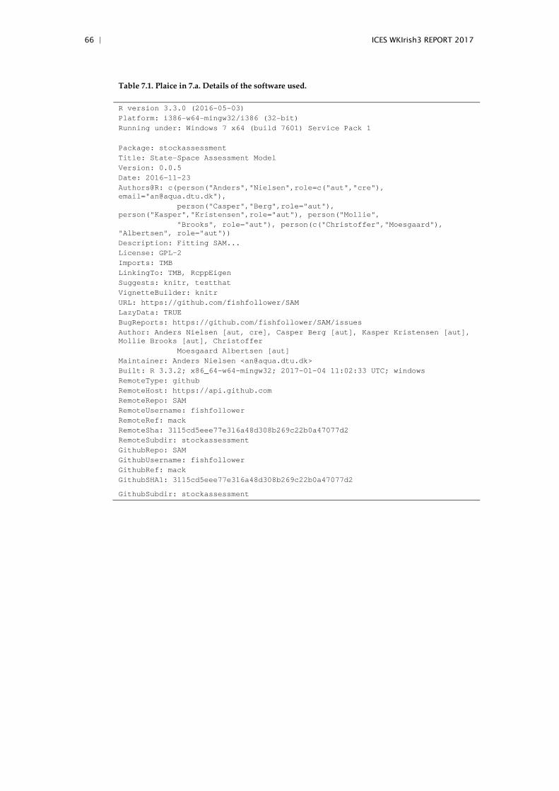
66 | ICES WKIrish3 REPORT 2017
Table 7.1. Plaice in 7.a. Details of the software used.
R version 3.3.0 (2016-05-03) Platform: i386-w64-mingw32/i386 (32-bit) Running under: Windows 7 x64 (build 7601) Service Pack 1 Package: stockassessment Title: State-Space Assessment Model Version: 0.0.5 Date: 2016-11-23 Authors@R: c(person("Anders","Nielsen",role=c("aut","cre"), email="[email protected]"), person("Casper","Berg",role="aut"), person("Kasper","Kristensen",role="aut"), person("Mollie", "Brooks", role="aut"), person(c("Christoffer","Moesgaard"), "Albertsen", role="aut")) Description: Fitting SAM... License: GPL-2 Imports: TMB LinkingTo: TMB, RcppEigen Suggests: knitr, testthat VignetteBuilder: knitr URL: https://github.com/fishfollower/SAM LazyData: TRUE BugReports: https://github.com/fishfollower/SAM/issues Author: Anders Nielsen [aut, cre], Casper Berg [aut], Kasper Kristensen [aut], Mollie Brooks [aut], Christoffer Moesgaard Albertsen [aut] Maintainer: Anders Nielsen <[email protected]> Built: R 3.3.2; x86_64-w64-mingw32; 2017-01-04 11:02:33 UTC; windows RemoteType: github RemoteHost: https://api.github.com RemoteRepo: SAM RemoteUsername: fishfollower RemoteRef: mack RemoteSha: 3115cd5eee77e316a48d308b269c22b0a47077d2 RemoteSubdir: stockassessment GithubRepo: SAM GithubUsername: fishfollower GithubRef: mack GithubSHA1: 3115cd5eee77e316a48d308b269c22b0a47077d2
GithubSubdir: stockassessment
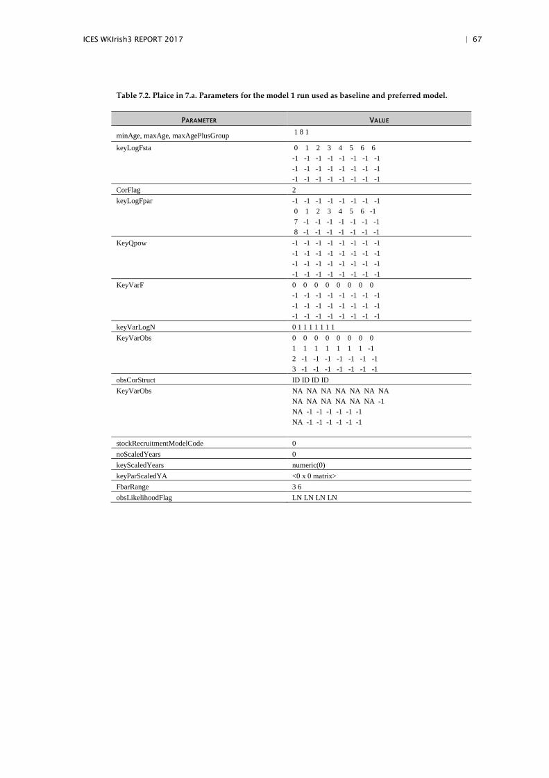
ICES WKIrish3 REPORT 2017 | 67
Table 7.2. Plaice in 7.a. Parameters for the model 1 run used as baseline and preferred model.
PARAMETER VALUE
minAge, maxAge, maxAgePlusGroup 1 8 1
keyLogFsta
0 1 2 3 4 5 6 6 -1 -1 -1 -1 -1 -1 -1 -1 -1 -1 -1 -1 -1 -1 -1 -1 -1 -1 -1 -1 -1 -1 -1 -1
CorFlag 2 keyLogFpar -1 -1 -1 -1 -1 -1 -1 -1
0 1 2 3 4 5 6 -1 7 -1 -1 -1 -1 -1 -1 -1 8 -1 -1 -1 -1 -1 -1 -1
KeyQpow -1 -1 -1 -1 -1 -1 -1 -1 -1 -1 -1 -1 -1 -1 -1 -1 -1 -1 -1 -1 -1 -1 -1 -1 -1 -1 -1 -1 -1 -1 -1 -1
KeyVarF 0 0 0 0 0 0 0 0 -1 -1 -1 -1 -1 -1 -1 -1 -1 -1 -1 -1 -1 -1 -1 -1 -1 -1 -1 -1 -1 -1 -1 -1
keyVarLogN 0 1 1 1 1 1 1 1 KeyVarObs 0 0 0 0 0 0 0 0
1 1 1 1 1 1 1 -1 2 -1 -1 -1 -1 -1 -1 -1 3 -1 -1 -1 -1 -1 -1 -1
obsCorStruct ID ID ID ID KeyVarObs NA NA NA NA NA NA NA
NA NA NA NA NA NA -1 NA -1 -1 -1 -1 -1 -1 NA -1 -1 -1 -1 -1 -1
stockRecruitmentModelCode 0 noScaledYears 0 keyScaledYears numeric(0) keyParScaledYA <0 x 0 matrix> FbarRange 3 6 obsLikelihoodFlag LN LN LN LN

68 | ICES WKIrish3 REPORT 2017
Figure 7.1. Plaice in 7.a. Baseline model estimates of survey selectivity for the UK Quarter 3 beam trawl survey and the NI Quarter 1 and Quarter 4 surveys.
Figure 7.2. Plaice in 7.a. Landings and discards partial fishing mortality estimated by the baseline model.

ICES WKIrish3 REPORT 2017 | 69
Figure 7.3. Plaice in 7.a. Residuals in fits to catch and survey data from the baseline model.
Figure 7.4. Plaice in 7.a. Retrospective assessments for years 2005–2015 from the baseline model.

70 | ICES WKIrish3 REPORT 2017
Figure 7.5. Plaice in 7.a. Effect of using different combinations of surveys.
Figure 7.6. Plaice in 7.a. Impact of alternative methods of discard reconstruction on key model outputs.

ICES WKIrish3 REPORT 2017 | 71
Figure 7.7. Plaice in 7.a. Impact of alternative discard survival rates on key model outputs. Note that Catch and Fbar refer to the portion of the catch which does not survive.
Figure 7.8. Plaice in 7.a. Impact of alternative natural mortality assumptions on key model out-puts.

72 | ICES WKIrish3 REPORT 2017
Figure 7.9. Plaice in 7.a. Impact of alternative survey maturity ogives assumptions on key model outputs.
Figure 7.10. Plaice in 7.a. Impact of alternative F random walk assumptions on key model outputs.

ICES WKIrish3 REPORT 2017 | 73
Figure 7.11. Plaice in 7.a. Impact of assessment length on key model outputs.
Figure 7.12. Plaice in 7.a. Comparison of the baseline model with the previous model used by WGCSE and the annual egg production method estimates (Armstrong et al., 2012).
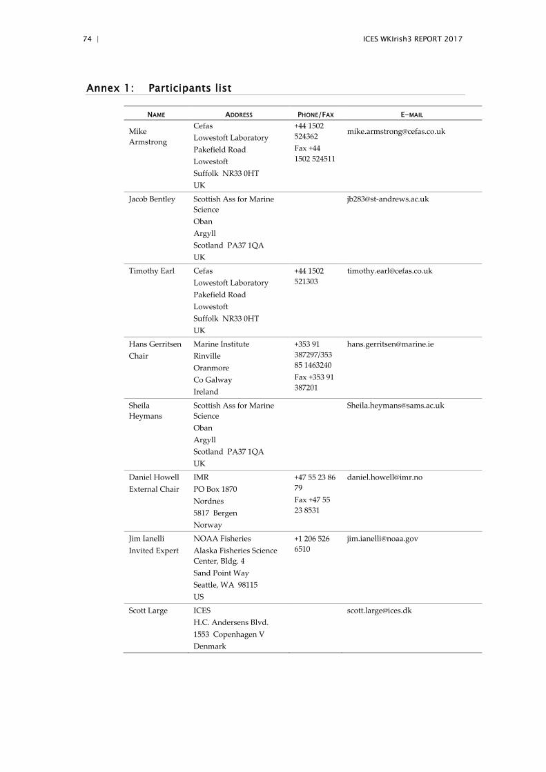
74 | ICES WKIrish3 REPORT 2017
Annex 1: Participants list
NAME ADDRESS PHONE/FAX E-MAIL
Mike Armstrong
Cefas Lowestoft Laboratory Pakefield Road Lowestoft Suffolk NR33 0HT UK
+44 1502 524362 Fax +44 1502 524511
Jacob Bentley Scottish Ass for Marine Science Oban Argyll Scotland PA37 1QA UK
Timothy Earl Cefas Lowestoft Laboratory Pakefield Road Lowestoft Suffolk NR33 0HT UK
+44 1502 521303
Hans Gerritsen Chair
Marine Institute Rinville Oranmore Co Galway Ireland
+353 91 387297/353 85 1463240 Fax +353 91 387201
Sheila Heymans
Scottish Ass for Marine Science Oban Argyll Scotland PA37 1QA UK
Daniel Howell External Chair
IMR PO Box 1870 Nordnes 5817 Bergen Norway
+47 55 23 86 79 Fax +47 55 23 8531
Jim Ianelli Invited Expert
NOAA Fisheries Alaska Fisheries Science Center, Bldg. 4 Sand Point Way Seattle, WA 98115 US
+1 206 526 6510
Scott Large ICES H.C. Andersens Blvd. 1553 Copenhagen V Denmark

ICES WKIrish3 REPORT 2017 | 75
NAME ADDRESS PHONE/FAX E-MAIL
Rebecca Lauerburg Invited Expert
University of Hamburg Institute of Hydrobiology and Fishery Olbersweg 24 Department of Biology 22767 Hamburg Germany
+49 40 42838-6609
Colm Lordan Marine Institute Rinville Oranmore Co Galway Ireland
+353 91 387 387 (or *200) Cell +35 876 995 708 Fax +353 91 387201
Matt Lundy Agri-Food and Biosciences Institute NI 18a Newforge Lane Belfast NI BT9 5PX UK
+44 2890255521
Alan McCulla Anglo North Irish Fish Producers’ Organisation The Harbour Kilkeel Co Down NI BT34 4AX UK
Claire Moore Marine Institute Rinville Oranmore Co Galway Ireland
Sara Jane Moore
Marine Institute Rinville Oranmore Co Galway Ireland
+353 91 387298 Fax +353 91 387201
Pieter-Jan Schön
Agri-Food and Biosciences Institute NI 18a Newforge Lane Belfast NI BT9 5PX UK
+44 28 90255015 Fax +44 28 90255004
Jonathan Shrives
European Commission Directorate-General for Maritime Affairs and Fisheries Unit C.2 - Atlantic and outermost regions J79 02/03 1049 Brussels Belgium
+32 229-62681

76 | ICES WKIrish3 REPORT 2017
NAME ADDRESS PHONE/FAX E-MAIL
Pia Schuchert Agri-Food and Biosciences Institute NI 18a Newforge Lane Belfast NI BT9 5PX UK
Robert Thorpe Cefas Pakefield Road Lowestoft Suffolk NR33 0HT UK
Jonathan White Marine Institute Rinville, Oranmore Co Galway Ireland

ICES WKIrish3 REPORT 2017 | 77
Annex 2: Agenda
Agenda WKIrish3 30 January – 3 February 2017, Marine Institute, Galway, Ireland
Monday Tuesday Wednesday Thursday Friday
0900-1100start 10:00Introductions etc.
WHG: present WD, agree on work required during WS
Update on all stocks
Present work done and final conclusions
Reference points
coffee
1115-1300HAD: present WD, agree on work required during WS
HER: present WD, agree on work required during WS
Subgroups all stocks
Present work done and final conclusions
Reference points
lunch
1400-1600COD: present WD, agree on work required during WS
Subgroups all stocks
Present work done and final conclusions
Reference pointsRecommendations, stock annex and report
coffee
1615-1800PLE: present WD, agree on work required during WS
Subgroups all stocks
Present work done and final conclusions
Reference pointsRecommendations, stock annex and report
plenarysubgroups

78 | ICES WKIrish3 REPORT 2017
Annex 3: Radiocarbon (14C) activities in gadoid Otoliths
Stella Heymans (SAMS) presented work on 14C activities in gadoid otoliths that could be used to help inform on migration and stock boundaries.
WKIrish3 would support a proposal for the use the Sellafield 14C signal to investigate the possibility of southward migration of gadoids, such as cod and whiting from the Irish Sea to the Celtic Sea. Initial studies performed by SAMS/SUERC have shown that the signal in 14C between the Irish Sea and the Celtic Sea are substantially differ-ent, and if it was possible to use this signal either for stock movement or individual movement (via age rings in the otoliths), it would improve our understanding of spe-cifically the whiting stocks in the Irish Sea and their possible movement to the Celtic Sea.
In the UK, the Sellafield nuclear fuel reprocessing facility is authorised to discharge waste 14C to the marine environment. Low-level radioactive effluent containing 14C is discharged via pipelines that extend 2.1 km offshore into the Irish Sea. 14C is released primarily as inorganic carbon and is incorporated into the dissolved inorganic carbon (DIC) component of seawater (Begg et al., 1991; 1992; Begg, 1992; Cook et al., 1995). >99% of Sellafield 14C dispersed through the North Channel (Gulliver et al., 2001).
Sellafield 14C discharges are made in addition to existing “background” inputs of 14C from natural production and fallout from atmospheric testing of nuclear weapons in the 1950s and early 1960s. The background activities range from 248 ± 1.0 Bq kg–1 C in 1995 (Cook et al., 1998) to 249 ± 0.8 Bq kg–1 C for 2014 (Tierney et al., 2016a). Any 14C activities which are higher than these background activities in UK waters can be de-fined as enriched and the only significant source of additional 14C to waters on the UK west coast is Sellafield.
14C enters the marine foodweb via the efficient uptake of soluble 14C in DIC during photosynthesis by primary producing organisms, mainly phytoplankton (Muir et al., 2017; Tierney et al., 2017). Enriched 14C activities have been found in a range of ma-rine species occupying the lowest (phytoplankton) to middle-upper (e.g. piscivorous fish) trophic levels in the Irish Sea (Muir et al., 2017) and West of Scotland (Tierney et al., 2017) marine environments. The uptake of Sellafield-derived 14C in carbonate producing organisms, specifically molluscs, has also been investigated (Cook et al., 2004; Muir et al., 2015; Tierney et al., 2016). Similarly to 14C uptake by molluscs, fish will produce otoliths with a 14C signature representative of the environment it inhab-its. In UK waters, the Irish Sea has the highest 14C activity. Net northerly dispersion has resulted in enriched activities being found in the West of Scotland and lower, closer to background, activities are expected in the Celtic Sea.
In the first instance, a small number of cod otoliths (twelve) were analysed for 14C activity to investigate differences in 14C activity in these different UK coastal areas and to consider the possible migration of immature Irish Sea cod to other areas. The results are shown in Table 1. Irish Sea otolith 14C activity was highest. The east basin was more variable with proximity to the pipelines affecting activity. The sample with the highest activity (802 ± 3 Bq kg–1 C) comes from an individual caught due west of Sellafield, the other two samples (413 ± 2 and 349 ± 2 Bq kg–1 C) come from fish caught further south. The large difference in 14C activity suggests that these immature fish had not moved any real distance by this stage of their lives. The west basin ap-pears to be more consistent (415–422 Bq kg–1 C), which is expected due to dilution and subsequent dispersion of discharged 14C. These activities are comparable to pub-

ICES WKIrish3 REPORT 2017 | 79
lished 14C activities for Irish Sea shells and organisms (Cook et al., 1998; 2004; Muir et al., 2015; 2017; Tierney et al., 2016).
Two of the West of Scotland otolith samples come from fish caught relatively far north and therefore have enriched activities which are only slightly above back-ground (252 ± 1 and 256 ± 1 Bq kg–1 C). The third West of Scotland otolith has a higher activity (265 ± 1 Bq kg–1 C) and is comparable to activities measured in West of Scot-land shells and organisms (Tierney et al., 2016; Tierney et al., 2017).
The Celtic Sea activities are higher than would be expected and warrant further in-vestigation. The activities measured indicate that either 14C is being transported southwards through the St Georges Channel, which is unlikely based on previous studies (Cook et al., 1998; Gulliver et al., 2001). The alternative is that these cod have spent a period of time in the Irish Sea. Thus we can use the 14C signal to investigate the possibility of southward migration of gadoids, such as cod and whiting from the Irish Sea. To undertake this study we would need to measure 14C from otoliths ob-tained in both the Irish and Celtic seas and ambient seawater for DIC 14C activity. Larger otoliths could also be used to address an individual’s movement through time; i.e. higher activities in the Irish Sea vs. lower activities in the Celtic Sea.
Table 1. 14C activities in cod otoliths.
YEAR AREA LATITUDE LONGITUDE OTOLITH
WEIGHT (MG)
OTOLITH 14C
ACTIVITY (BQ KG–1 C)
2005 Irish Sea E 54.330 -3.924 71.5 802 ± 3
2005 Irish Sea E 53.515 -4.235 44.7 413 ± 2
2005 Irish Sea E 52.558 -6.040 156.0 349 ± 2
2005 Irish Sea W 54.117 -5.532 41.3 415 ± 2
2005 Irish Sea W 53.958 -5.692 41.6 426 ± 2
2005 Irish Sea W 53.583 -5.899 31.9 422 ± 2
2010 W Scotland 55.767 -9.081 1210.0 265 ± 1
2010 W Scotland 58.795 -6.215 7340.0 252 ± 1
2010 W Scotland 58.134 -6.127 3338.0 256 ± 1
2010 N Celtic Sea 51.460 -8.505 117.0 273 ± 1
2010 N Celtic Sea 51.590 -7.464 166.0 292 ± 2
2010 N Celtic Sea 51.348 -8.108 148.0 273 ± 1

80 | ICES WKIrish3 REPORT 2017
Annex 4: Reconstructing Irish Sea plaice discard numbers
Tim Earl, Simon Fischer and Mike Armstrong
9 February 2017
Introduction
WKIrish2 (ICES, 2016a) and WKFLAT (ICES, 2011) identified the importance of mod-elling discards within this stock because of the large proportion of the catch that is currently discarded; in the period 2011–2015 66% of catch by weight was discarded (ICES, 2016b). Discards have been routinely sampled since 2004 by UK, Ireland and Belgium to provide raised estimates of discard numbers-at-age, but there is limited data on discard levels before 2004. WKIrish2 identified the following sources of data:
• Discard numbers-at-age since 2004 (shown as proportions in Figure A1); • Discard numbers-at-length since 2004 (Figures A2–A4); • UK beam trawl survey data showing changing length-at-age since 1993
(Figure A5); • Legislation setting a minimum landing size (MLS) of 250 mm in 1981
(Council Regulation (EEC) No 2527/80) and 270 mm in 1998 (Council Regulation (EEC) No 850/98);
• A report showing numbers discarded and retained by length and age for a set of UK (England) vessels sampled in 1993 during a selectivity investiga-tion in the eastern Irish Sea during the period when the MLS was 250 mm (Emberton et al., 1995);
• A report giving observer data from 1998/1999 (Commission 2002) showing overall discard rates of 69–83% by number in 1999 and 2000 for UK (Northern Ireland) single and multiple rig Nephrops trawlers, and 91–100% for UK(NI) midwater trawlers.
Observer data from 2004–2006 are based on relatively few trips with data on plaice (Figure A6).
From these data sources the following conclusions can be drawn:
• A large proportion of the discards occur below the minimum landing size, and this was still true when the minimum landing size was 250 mm based on a single study.
• The growth rate of plaice in the Irish Sea has been declining over time, so constant selectivity and discarding ogive by length will have led to an in-creasing trend in discard rates at-age.
• Discards have made up a substantial proportion of the catch during the time period back to the early 1990s for which reports exist, although the rates decline going back in time due to the changes in growth and MLS. No direct evidence of discard rates prior to the early 1990s was available to WKIrish.

ICES WKIrish3 REPORT 2017 | 81
Scenarios
Three possible scenarios are investigated as potential discard reconstructions to be used in stock assessment models:
• Low discards: The decline in discard fractions at-age between 2008 and 2004 is extrapolated backwards to a point where the fraction is zero. No discarding occurred before that.
• Medium discards: The method is described in more detail below. It creates a discard time-series that is consistent with the key conclusions drawn from the historical data.
• High discards: The discard fractions at-age between 2008 and 2004 are as-sumed to be typical of the entire period. WKIrish3 noted that it was sensi-tive to the reference period (i.e. changing 2008–2004 to 2009–2005 increased catches in some years by around 70%)
The high and low discards scenarios do not fit well with the key conclusions drawn from the review of discards, and are treated as upper and lower bounds that can be used in sensitivity testing the assessment model. The low discards option requires an extrapolation of a trend that is heavily driven by 2004–2006 data which are based on relatively few observer trips (Figure A6) and is likely to be extremely inaccurate, as well as invoking an implausible assumption of zero discarding in earlier years. The medium discards scenario will be taken forward as a potential input to the assess-ment used for management.
Medium discards reconstruction method
The intention of this method was to derive historical discards numbers using a meth-od that is data-driven as far as possible, although some important assumptions are required. The data sources available suggest a strong relationship across age groups between mean size-at-age and the fraction of the catch that is discarded. Data on length-at-age distributions of landings were not available for the entire time-series, and so landings weights-at-age are used as a proxy. These landings data have high variability between years, and so a lowess smoother (with smoothing span 0.15 cho-sen by eye) was fitted to remove the intra-annual variability, while retaining infor-mation about the longer term trends. The fit of the smoother is shown in Figure 1 and a comparison of the trends across all year is shown in Figure 2.
A plot of the relationship between the smoothed landings weights and discard frac-tions at-age based on the observer data from 2004 onwards is shown in Figure 3. Each point represents a combination of age and year, colour indicates ages 1:8+. Existing data show little or no retention of fish below the MLS (Commission 2002; Appendix Figures A2–A4), but some discarding above the MLS. The line plotted in Figure 3 therefore indicates a lower bound on discards (fitted by eye rather than a best fit) to capture the discarding due only to the MLS and not influenced by other factors (e.g. economic) that may have been responsible for higher rates of discarding in each age class in recent years. This means that the discard fractions estimated from this rela-tionship are likely to be an underestimate of the discard fractions.
Prior to 1998, the MLS was 250 mm, rather than 270 mm. Using the length–weight relationship used by the NI survey (a=8E-6, b=3.0572) the change in length would equate to a change in weight of 40 g, and so prior to 1998 the logistic fit was shifted to the left by this amount.

82 | ICES WKIrish3 REPORT 2017
The relationships between smoothed landings weights and discard fraction was used to estimate the discard fraction prior to 2004, and the estimated proportions are shown in Figure 4. For ages 3–8+, discard numbers prior to 2004 are estimated by raising the landings numbers by the discard fraction. The discard fractions at-ages 1 and 2 exceed 90% at some points prior to the start of discards data, implying a raising factor of at least ten times would be applied to landings to estimate discards. In years with zero landings at these ages, no figure for discards can be obtained. These factors would substantially amplify the errors in landings estimation, and create very noisy estimate of discard numbers (and hence catch numbers) at these youngest ages, and so an alternative approach is needed to estimate discard numbers at these ages.
Figure 1. Plaice 7.a. Landings weight-at-age (red) and a lowess smoother (blue) fitted to the data.

ICES WKIrish3 REPORT 2017 | 83
Figure 2. Plaice 7.a. Smoothed landings weight-at-age. Note that in some years there were no samples of age 1 fish in the landings, which is indicated by the breaks in this line.
Figure 3. Plaice 7.a. Relationship between smoothed landings weights and proportion discarded, showing a logistic function fitted as a lower bound (black line).
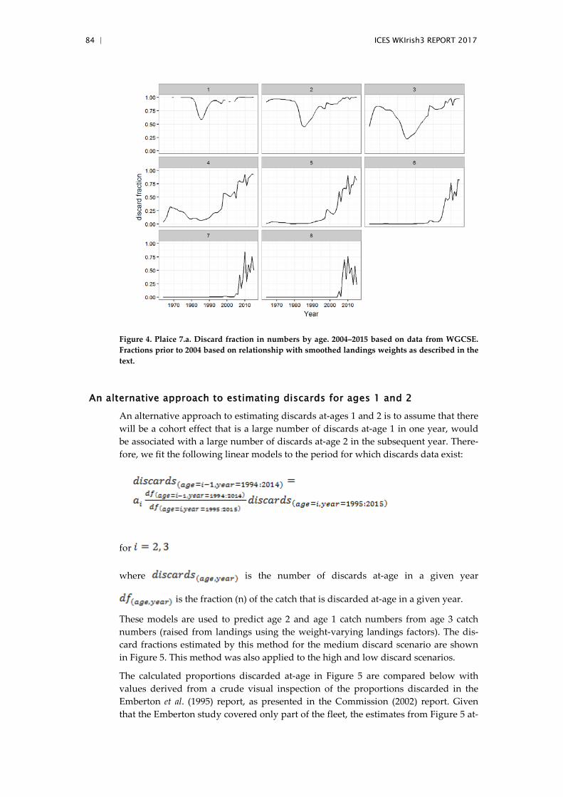
84 | ICES WKIrish3 REPORT 2017
Figure 4. Plaice 7.a. Discard fraction in numbers by age. 2004–2015 based on data from WGCSE. Fractions prior to 2004 based on relationship with smoothed landings weights as described in the text.
An alternative approach to estimating discards for ages 1 and 2
An alternative approach to estimating discards at-ages 1 and 2 is to assume that there will be a cohort effect that is a large number of discards at-age 1 in one year, would be associated with a large number of discards at-age 2 in the subsequent year. There-fore, we fit the following linear models to the period for which discards data exist:
for
where is the number of discards at-age in a given year
is the fraction (n) of the catch that is discarded at-age in a given year.
These models are used to predict age 2 and age 1 catch numbers from age 3 catch numbers (raised from landings using the weight-varying landings factors). The dis-card fractions estimated by this method for the medium discard scenario are shown in Figure 5. This method was also applied to the high and low discard scenarios.
The calculated proportions discarded at-age in Figure 5 are compared below with values derived from a crude visual inspection of the proportions discarded in the Emberton et al. (1995) report, as presented in the Commission (2002) report. Given that the Emberton study covered only part of the fleet, the estimates from Figure 5 at-

ICES WKIrish3 REPORT 2017 | 85
ages 1–3 are not completely out of line with Emberton, though are much lower at-ages 4 and 5.
Source
% discarded at age
Age 1 Age 2 Age 3 Age 4 Age 5
Present study (Figure 5) estimates for 1993
94% 78% 51% 21% 6%
Emberton et al., 1995/ Commission 2012
~100% 60–80% 50–65% 40–50% 20–40%
Figure 5. Plaice 7.a. Discard fraction in numbers by age. 2004–2015 based on data from WGCSE. Fractions prior to 2004 based on relationship with smoothed landings weights as described in the text, with alternative approach for ages 1 and 2.
Reconstructed time-series
Figures 6–8 show the total weight of discards implied by each of the three discard scenarios, low, medium and high respectively.
Given the lack of information about the MLS prior to 1981, or any survey data to in-dicate if changes in mean weight-at-age in landings are related to changes in discard-ing ogives rather than growth, it is recommended to use data from 1981–present for the baseline stock assessment run, and consider the inclusion of the earlier period as a sensitivity run.

86 | ICES WKIrish3 REPORT 2017
Figure 6. Plaice 7.a. Discards reconstruction from the low discards scenario (green), compared to discards data (red) and landings data (blue).
Figure 7. Plaice 7.a. Discards reconstruction from the medium discards scenario (green), compared to discards data (red) and landings data (blue).
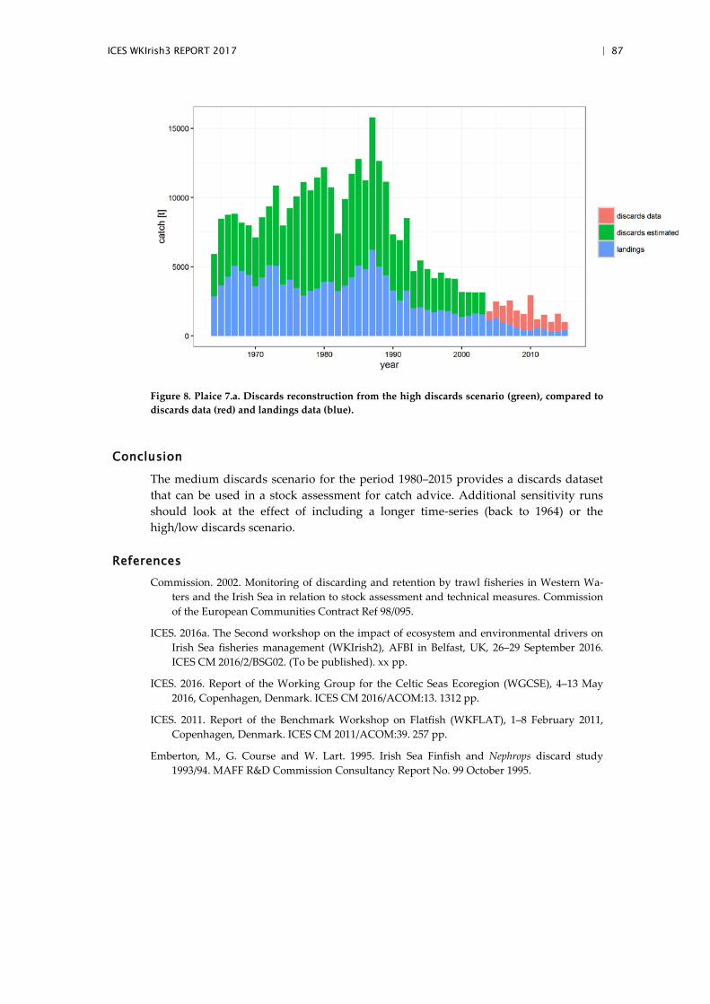
ICES WKIrish3 REPORT 2017 | 87
Figure 8. Plaice 7.a. Discards reconstruction from the high discards scenario (green), compared to discards data (red) and landings data (blue).
Conclusion
The medium discards scenario for the period 1980–2015 provides a discards dataset that can be used in a stock assessment for catch advice. Additional sensitivity runs should look at the effect of including a longer time-series (back to 1964) or the high/low discards scenario.
References Commission. 2002. Monitoring of discarding and retention by trawl fisheries in Western Wa-
ters and the Irish Sea in relation to stock assessment and technical measures. Commission of the European Communities Contract Ref 98/095.
ICES. 2016a. The Second workshop on the impact of ecosystem and environmental drivers on Irish Sea fisheries management (WKIrish2), AFBI in Belfast, UK, 26–29 September 2016. ICES CM 2016/2/BSG02. (To be published). xx pp.
ICES. 2016. Report of the Working Group for the Celtic Seas Ecoregion (WGCSE), 4–13 May 2016, Copenhagen, Denmark. ICES CM 2016/ACOM:13. 1312 pp.
ICES. 2011. Report of the Benchmark Workshop on Flatfish (WKFLAT), 1–8 February 2011, Copenhagen, Denmark. ICES CM 2011/ACOM:39. 257 pp.
Emberton, M., G. Course and W. Lart. 1995. Irish Sea Finfish and Nephrops discard study 1993/94. MAFF R&D Commission Consultancy Report No. 99 October 1995.
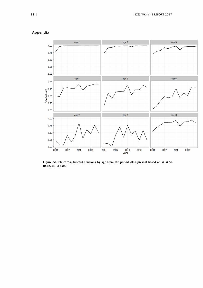
88 | ICES WKIrish3 REPORT 2017
Appendix
Figure A1. Plaice 7.a. Discard fractions by age from the period 2004–present based on WGCSE (ICES, 2016) data.

ICES WKIrish3 REPORT 2017 | 89
Figure A2. Plaice 7.a. Length distributions of discarded and retained catches from UK(E&W). Source: ICES (2016).

90 | ICES WKIrish3 REPORT 2017
Figure A3. Plaice 7.a. Length distributions of discarded and retained catches from Ireland. Source: ICES (2016).

ICES WKIrish3 REPORT 2017 | 91
Figure A4. Plaice 7.a. Length distributions of discarded and retained catches from Belgium. Source: ICES (2016).

92 | ICES WKIrish3 REPORT 2017
Figure A5. Plaice 7.a. Length-at-age over time from the UKBTS, broken down by sex and area within the Irish Sea. Source: ICES (2016).

ICES WKIrish3 REPORT 2017 | 93
Figure A6. Plaice 7.a. Numbers of observer trips in the Irish Sea, by country and gear since 2004, where plaice were recorded (Ireland is all trips; OTB: bottom otter trawl).

94 | ICES WKIrish3 REPORT 2017
Figure A6. Plaice in 7.a. Catch-at-age distributions for beam trawl, otter trawl, Nephrops trawl and anchor seine gear types for plaice in the Irish Sea between October 1993 and August 1994, sampled as part of the Emberton et al. (1995) study but as given in the Commission (2002) report (presumably through reworking of the data by SeaFish).

ICES WKIrish3 REPORT 2017 | 95
Annex 5: Plaice in 7.a reference points
Read in assessment outputs
library(msy)
library(icesAdvice)
library(FLCore)
withr::with_libpaths(new = paste0(.libPaths(), "/../library2"),
library("stockassessment"))
path <- "C:/Ple7a Benchmark/Models/SAM/"
load(paste0(path, "SAM/fit_b9.rdata")) ## Model fit
load(paste0(path, "da-ta/new_stocks/ple7a_dis_app5_1981.RData")) ## Input Ple7a
SAM_to_FLStock <- function(stock_object, ### FLStock object
SAM_object ### SAM object
){
### enter stock numbers estimations
stock.n(stock_object)[] <- exp(SAM_object$pl$logN)
### get ages available in F@age estimations
### (neccessary because of possible linked F patterns at age)
ages <- SAM_object$conf$keyLogFsta[1, ] + 1
### enter F estimations
harvest(stock_object)[] <- exp(SAM_object$pl$logF)[ages, ]
return(stock_object)
}
ple7a_proj <- SAM_to_FLStock(stock,fit_b9)
plot(rec(ple7a_proj),type='l')
Figure 13. Plaice in 7.a. Recruitment time-series.
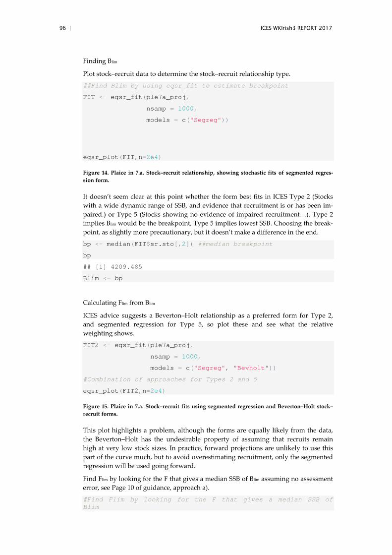
96 | ICES WKIrish3 REPORT 2017
Finding Blim
Plot stock–recruit data to determine the stock–recruit relationship type.
##Find Blim by using eqsr_fit to estimate breakpoint
FIT <- eqsr_fit(ple7a_proj,
nsamp = 1000,
models = c("Segreg"))
eqsr_plot(FIT,n=2e4)
Figure 14. Plaice in 7.a. Stock–recruit relationship, showing stochastic fits of segmented regres-sion form.
It doesn’t seem clear at this point whether the form best fits in ICES Type 2 (Stocks with a wide dynamic range of SSB, and evidence that recruitment is or has been im-paired.) or Type 5 (Stocks showing no evidence of impaired recruitment…). Type 2 implies Blim would be the breakpoint, Type 5 implies lowest SSB. Choosing the break-point, as slightly more precautionary, but it doesn’t make a difference in the end.
bp <- median(FIT$sr.sto[,2]) ##median breakpoint
bp
## [1] 4209.485
Blim <- bp
Calculating Flim from Blim
ICES advice suggests a Beverton–Holt relationship as a preferred form for Type 2, and segmented regression for Type 5, so plot these and see what the relative weighting shows.
FIT2 <- eqsr_fit(ple7a_proj,
nsamp = 1000,
models = c("Segreg", "Bevholt"))
#Combination of approaches for Types 2 and 5
eqsr_plot(FIT2,n=2e4)
Figure 15. Plaice in 7.a. Stock–recruit fits using segmented regression and Beverton–Holt stock–recruit forms.
This plot highlights a problem, although the forms are equally likely from the data, the Beverton–Holt has the undesirable property of assuming that recruits remain high at very low stock sizes. In practice, forward projections are unlikely to use this part of the curve much, but to avoid overestimating recruitment, only the segmented regression will be used going forward.
Find Flim by looking for the F that gives a median SSB of Blim assuming no assessment error, see Page 10 of guidance, approach a).
#Find Flim by looking for the F that gives a median SSB of Blim

ICES WKIrish3 REPORT 2017 | 97
#Page 10 of guidance, approach a)
SIM0 <- eqsim_run(FIT, #for finding Flim
bio.years = c(2006:2015),
sel.years = c(2006:2015),
Fcv=0, ##
Fphi=0, ##Default from WKMSYREF4
Blim=Blim,
Bpa=Bpa,
Fscan = seq(0,1.2,len=40),
verbose=FALSE,
extreme.trim=c(0.05,0.95),
Btrigger=0)
eqsim_plot_range(SIM0, type="ssb")
Figure 16. Plaice in 7.a. Relationship between Median SSB and F assuming no assessment error.
Reading across from our Blim gives:
Flim <- approx(SIM0$rbp[SIM0$rbp$variable=="Spawning–stock bio-mass","p50"],
SIM0$rbp[SIM0$rbp$variable=="Spawning-stock bio-mass","Ftarget"],
Blim)$y
Flim
## [1] 0.4821977
Fpa and Bpa
Using the CVs from the assessment outputs, we can calculate the PA reference points.
SSBcv <- mean(ssbtable(fit_b9)["2015",3]/ssbtable(fit_b9)["2015",1]-1)
SSBcv
## [1] 0.383187
Bpa <- Bpa(Blim, SSBcv)
Bpa
## [1] 7906.481
Fcv <- mean(fbartable(fit_b9)["2015",3]/fbartable(fit_b9)["2015",1]-1)
Fcv
## [1] 0.3950325

98 | ICES WKIrish3 REPORT 2017
Calculating FMSY, step 1
Step 1, from page 13 of guidance, FMSY without Btrigger
SIM1 <- eqsim_run(FIT,
bio.years = c(2006:2015),
sel.years = c(2006:2015),
Fcv=Fcv,
Fphi=0.423, ##Default from WKMSYREF4
Blim=Blim,
Bpa=Bpa,
Fscan = seq(0,1.2,len=40),
verbose=FALSE,
Btrigger=0,
extreme.trim=c(0.05,0.95))
Fmsy.notrig <- SIM1$Refs2["lanF","meanMSY"]
Fmsy.notrig
## [1] 0.1538462
Fmsy.notrig < Fpa #True, so MSY consistent with PA
## [1] TRUE
eqsim_plot(SIM1,catch=TRUE)
eqsim_plot_range(SIM1, type="median")
eqsim_plot_range(SIM1, type="ssb")
So FMSY with no trigger is 0.154, and this is consistent with the precautionary ap-proach.
Calculating FMSY, step 2
Step 2, from page 13 of guidance, select MSY Btrigger.
fbar(ple7a_proj) < Fmsy.notrig
## An object of class "FLQuant"
## , , unit = unique, season = all, area = unique
##
## year
## age 1981 1982 1983 1984 1985 1986 1987 1988 1989 1990 1991
## all FALSE FALSE FALSE FALSE FALSE FALSE FALSE FALSE FALSE FALSE FALSE
## year

ICES WKIrish3 REPORT 2017 | 99
## age 1992 1993 1994 1995 1996 1997 1998 1999 2000 2001 2002
## all FALSE FALSE FALSE FALSE FALSE FALSE FALSE FALSE FALSE FALSE FALSE
## year
## age 2003 2004 2005 2006 2007 2008 2009 2010 2011 2012 2013
## all FALSE TRUE FALSE FALSE FALSE FALSE TRUE FALSE TRUE TRUE TRUE
## year
## age 2014 2015
## all TRUE TRUE
##
## units: f
F below candidate FMSY for last five years, so go down in flowchart (page 16)
eqsim_plot_range(SIM1, type="ssb") ##Lower=11232 >> Bpa, down in flowchart
Lower 5%ile of Biomass much bigger than Bpa, so go down in flowchart. There’s no current Btrigger to compare to, so have a look at which options make more sense; seems sensible to go to bottom left box, in which case go right, to choose MSY Btrigger as the lower 5%ile of current biomass.
Btrigger <-ssbtable(fit_b9)["2015","Low"]
Btrigger <- 10392.13 #lower 5% of current SSB
Calculating FMSY, step 3
Step 3, from page 13 of guidance, evaluate whole advice rule including Btrigger.
SIM.trig <- eqsim_run(FIT,
bio.years = c(2006:2015),
sel.years = c(2006:2015),
Fcv=Fcv, ##
Fphi=0.423, ##Default from WKMSYREF4
Blim=Blim,
Bpa=Bpa,
Fscan = seq(0,1.2,len=40),
verbose=FALSE,
Btrigger=Btrigger,
extreme.trim=c(0.05,0.95))
eqsim_plot(SIM.trig,catch=TRUE)

100 | ICES WKIrish3 REPORT 2017
eqsim_plot_range(SIM.trig, type="median")
eqsim_plot_range(SIM.trig, type="ssb") ##lower percentile=11274 >> Blim

ICES WKIrish3 REPORT 2017 | 101
Annex 6: Diagnostics and stock summary plots

ASAP assessmentHans Gerritsen
February 02, 2017
R and FLR versions
library(FLCore)
## Warning: package 'FLCore' was built under R version 3.1.2
library(lattice)sessionInfo()
## R version 3.1.1 (2014-07-10)## Platform: i386-w64-mingw32/i386 (32-bit)#### locale:## [1] LC_COLLATE=English_Ireland.1252 LC_CTYPE=English_Ireland.1252## [3] LC_MONETARY=English_Ireland.1252 LC_NUMERIC=C## [5] LC_TIME=English_Ireland.1252#### attached base packages:## [1] stats graphics grDevices utils datasets methods base#### other attached packages:## [1] FLCore_2.5.20150309 MASS_7.3-33 lattice_0.20-29#### loaded via a namespace (and not attached):## [1] digest_0.6.8 evaluate_0.8.3 formatR_1.3 grid_3.1.1## [5] htmltools_0.2.6 knitr_1.12.3 rmarkdown_0.9.5 stats4_3.1.1## [9] stringr_0.6.2 tools_3.1.1 yaml_2.1.13
Read the stock object
First set the main directory and data and output directories
maindir <- '.'#datadir <- paste0(maindir,'/1_Data/LowestoftFiles')asapdir <- paste0(maindir,'/asap')outdir <- paste0(maindir,'/4_Outputs')
The ASAP assessment is not done in R, however it produces an rdat file with outputs
Note that in this asap assessment the first age is age 0, so be careful!
asap <- dget(file.path(asapdir,'run-final.rdat'))retrofiles <- paste0('run-final_',sprintf('%03d',0:8),'.rdat')retro <- lapply(retrofiles,FUN=function(x) dget(file.path(asapdir,x)))
1
102

pal <- c("#1B9E77", "#D95F02", "#7570B3", "#E7298A", "#66A61E", "#E6AB02","#A6761D", "#666666")for(i in 1:8) retro[[i]]$col <- pal[i]# years 2010 and 2014 converged but hessian was not positive# maybe leave out
#xsa resultsload('./4_Outputs/whg7a_xsa.Rdata')load('./4_Outputs/whg7a_stock.Rdata')
Some housekeeping
Some handy parameters to keep for later
years <- asap$parms$styr:asap$parms$endyrnyears <- length(years)ages <- 1:asap$parms$nages -1 # note the age offsetnages <- length(ages)nindices <- asap$parms$nindicesindices <- c('NI-Q1','NI-Q4','NI-MIK')fbarage <- asap$options$Freport.agemin:asap$options$Freport.agemax - 1 # note the age offset
A Function to save the plots
SavePlot0<-function(plotname,width=6,height=4){file <- file.path(outdir,paste0('whg7a_asap_',plotname,'.png'))dev.print(png,file,width=width,height=height,units='in',res=300,pointsize=8)
}
A bubble plot function
bubbles <- function(x,z,cex, key.space = 'right',...){maxz <- max(abs(z),na.rm=T)panel.fun <- function(x,z,subscripts,cex,...){
pt.cex <- sqrt(abs(z)/maxz)*cexpt.bg <- ifelse(z<0, '#FF000050','#00000050')lpoints(x,cex=pt.cex[subscripts],pch=21,fill=pt.bg[subscripts],col=1,...)
}text <- as.character(round(seq(maxz,-maxz,length=6),2))key = list(space = key.space, text = list(text),
points = list(pch = c(21), cex=sqrt(abs(seq(cex,-cex,length=6)))^2,fill = rep(c('#00000050','#FF000050'),each=3)),rep = FALSE)
xyplot(x,z=z,cex=cex,panel=panel.fun,key=key,...)}
Diagnostic plots
Observed and predicted catch
2
103
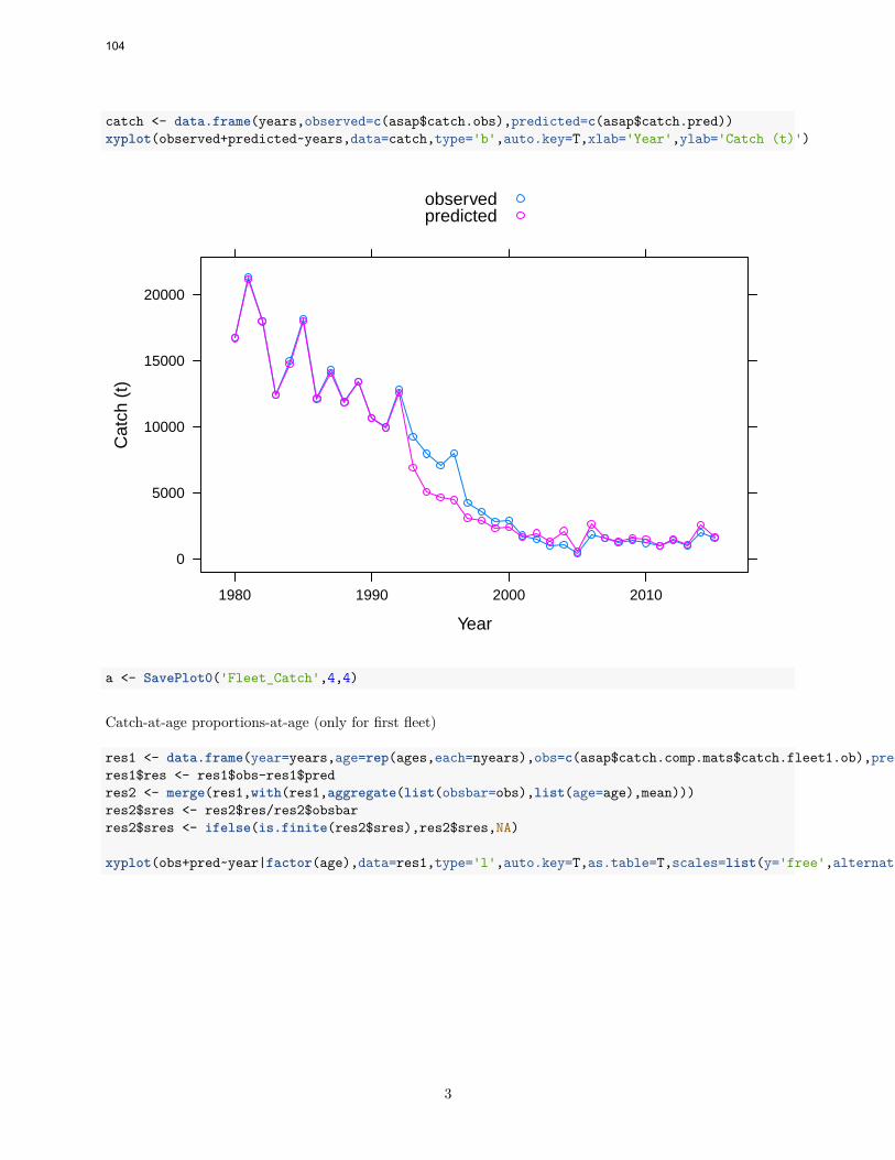
catch <- data.frame(years,observed=c(asap$catch.obs),predicted=c(asap$catch.pred))xyplot(observed+predicted~years,data=catch,type='b',auto.key=T,xlab='Year',ylab='Catch (t)')
Year
Cat
ch (
t)
0
5000
10000
15000
20000
1980 1990 2000 2010
observedpredicted
a <- SavePlot0('Fleet_Catch',4,4)
Catch-at-age proportions-at-age (only for first fleet)
res1 <- data.frame(year=years,age=rep(ages,each=nyears),obs=c(asap$catch.comp.mats$catch.fleet1.ob),pred=c(asap$catch.comp.mats$catch.fleet1.pr))res1$res <- res1$obs-res1$predres2 <- merge(res1,with(res1,aggregate(list(obsbar=obs),list(age=age),mean)))res2$sres <- res2$res/res2$obsbarres2$sres <- ifelse(is.finite(res2$sres),res2$sres,NA)
xyplot(obs+pred~year|factor(age),data=res1,type='l',auto.key=T,as.table=T,scales=list(y='free',alternating=F),ylab='Proportion-at-age')
3
104

year
Pro
port
ion−
at−
age
0.0
0.2
0.4
0.6
0
0.2
0.4
0.6
0.8
1
0.0
0.1
0.2
0.3
0.4
0.5
2
0.0
0.1
0.2
0.3
0.4
3
0.00
0.04
0.08
1980 2000
4
0.00
00.
010
0.02
0
1980 2000
5
0.00
00.
004
1980 2000
6
obspred
a <- SavePlot0('FleetCaaRes1')
panfun <- function(x, y) {panel.xyplot(x, y)panel.abline(h=0)
}xyplot(res~year|factor(age),data=res1,type='l',auto.key=T,as.table=T,ylab='Proportion-at-age residuals',panel=panfun)
4
105

year
Pro
port
ion−
at−
age
resi
dual
s
−0.2
0.0
0.2
0
1980199020002010
1 2
1980199020002010
3
1980199020002010
4 5
1980199020002010
−0.2
0.0
0.2
6
a <- SavePlot0('FleetCaaRes2')
bubbles(age~year,data=res1,z=res1$res,cex=5,xlab='Year',ylab='Age')
Year
Age
0
1
2
3
4
5
6
1980 1990 2000 2010
0.310.190.06−0.06−0.19−0.31
5
106

a <- SavePlot0('FleetResidualsAge',6,3.5)
bubbles(age~year,data=res2,z=res2$sres,cex=5,xlab='Year',ylab='Age')
Year
Age
0
1
2
3
4
5
6
1980 1990 2000 2010
3.92.340.78−0.78−2.34−3.9
a <- SavePlot0('FleetStResidualsAge',6,3.5)
Index fit
ind1 <- NULLfor(i in 1:nindices){
ind1 <- rbind(ind1, data.frame(years=years[asap$index.year.counter[[i]]],name=indices[i],observed=asap$index.obs[[i]],predicted=asap$index.pred[[i]]))}xyplot(observed+predicted~years|name,data=ind1,type='b',xlab='Year',ylab='Index',scales=list(alternating=1,y=list(relation='free')),auto.key=T)
6
107

Year
Inde
x
1000
2000
3000
4000
5000
1995 2000 2005 2010 2015
NI−Q1
2000
4000
6000
8000
1995 2000 2005 2010 2015
NI−Q4
020
040
060
080
0
1995 2000 2005 2010 2015
NI−MIK
observedpredicted
a <- SavePlot0('IndexFit')
Index proportions-at-age fit
#note: hard-coded for 2 indices with naares1 <- NULLfor(i in 1:2){
iob <- grep('ob',names(asap$index.comp.mats))[i]ipr <- grep('pr',names(asap$index.comp.mats))[i]res1 <- rbind(res1,data.frame(year=years,age=rep(ages,each=nyears),name=indices[i],obs=unlist(asap$index.comp.mats[iob]),pred=unlist(asap$index.comp.mats[ipr])))
}res1$obs <- ifelse(res1$obs==0 & res1$pred==0, NA,res1$obs)res1$pred <- ifelse(res1$obs==0 & res1$pred==0, NA,res1$pred)res1$res <- res1$obs-res1$predres2 <- merge(res1,with(res1,aggregate(list(obsbar=obs),list(age=age,name=name),mean,na.rm=T)))res2$sres <- res2$res/res2$obsbar#key <- simpleKey(text=c('obs','pred'),points=F,lines=T,space='right')key <- simpleKey(text=c('obs','pred'),points=F,lines=T,space='top')xyplot(obs+pred~year|paste(name,'Age',age),data=res1,type='l',key=key,scales=list(alternating=1),par.strip.text=list(cex=0.6),ylab='Proportion-at-age',layout=c(nages,2),as.table=T)
7
108

year
Pro
port
ion−
at−
age
0.0
0.2
0.4
0.6
0.8
NI−Q1 Age 0 NI−Q1 Age 1 NI−Q1 Age 2 NI−Q1 Age 3 NI−Q1 Age 4 NI−Q1 Age 5 NI−Q1 Age 6
0.0
0.2
0.4
0.6
0.8
1980 2000
NI−Q4 Age 0
1980 2000
NI−Q4 Age 1
1980 2000
NI−Q4 Age 2
1980 2000
NI−Q4 Age 3
1980 2000
NI−Q4 Age 4
1980 2000
NI−Q4 Age 5
1980 2000
NI−Q4 Age 6
obspred
a <- SavePlot0('IndexCaa',6,6)
panfun <- function(x, y) {panel.xyplot(x, y)panel.abline(h=0)
}xyplot(res~year|paste(name,'Age',age),data=res1,type='l',scales=list(alternating=1),par.strip.text=list(cex=0.6),ylab='Proportion-at-age',layout=c(nages,2),as.table=T,panel=panfun)
8
109

year
Pro
port
ion−
at−
age
−0.2
−0.1
0.0
0.1
0.2
NI−Q1 Age 0 NI−Q1 Age 1 NI−Q1 Age 2 NI−Q1 Age 3 NI−Q1 Age 4 NI−Q1 Age 5 NI−Q1 Age 6
−0.2
−0.1
0.0
0.1
0.2
1980 2000
NI−Q4 Age 0
1980 2000
NI−Q4 Age 1
1980 2000
NI−Q4 Age 2
1980 2000
NI−Q4 Age 3
1980 2000
NI−Q4 Age 4
1980 2000
NI−Q4 Age 5
1980 2000
NI−Q4 Age 6
a <- SavePlot0('IndexResAge',6,6)
res1 <- subset(res1,res!=0 & name!='NI-MIK')bubbles(age~year|name,data=res1,z=res1$res,cex=3,xlab='Year',ylab='Age',layout=c(1,2),scales=list(alternating=1),key.space='top')
9
110

Year
Age
0
1
2
3
4
5
6
1995 2000 2005 2010 2015
NI−Q10
1
2
3
4
5
6NI−Q4
0.260.160.05−0.05−0.16−0.26
a <- SavePlot0('IndexResidualsAge',3.1,6)
res2 <- subset(res2,sres!=0 & is.finite(sres))bubbles(age~year|name,data=res2,z=res2$sres,cex=3,xlab='Year',ylab='Age',layout=c(1,2),scales=list(alternating=1),key.space='top')
10
111
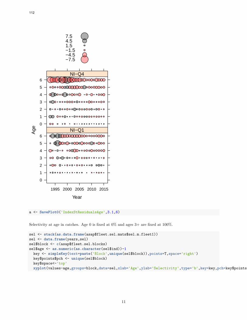
Year
Age
0
1
2
3
4
5
6
1995 2000 2005 2010 2015
NI−Q10
1
2
3
4
5
6NI−Q4
7.54.51.5−1.5−4.5−7.5
a <- SavePlot0('IndexStResidualsAge',3.1,6)
Selectivity at age in catches. Age 0 is fixed at 0% and ages 3+ are fixed at 100%.
sel <- stack(as.data.frame(asap$fleet.sel.mats$sel.m.fleet1))sel <- data.frame(years,sel)sel$block <- c(asap$fleet.sel.blocks)sel$age <- as.numeric(as.character(sel$ind))-1
key <- simpleKey(text=paste('Block',unique(sel$block)),points=T,space='right')key$points$pch <- unique(sel$block)key$space<-'top'xyplot(values~age,groups=block,data=sel,xlab='Age',ylab='Selectivity',type='b',key=key,pch=key$points$pch)
11
112
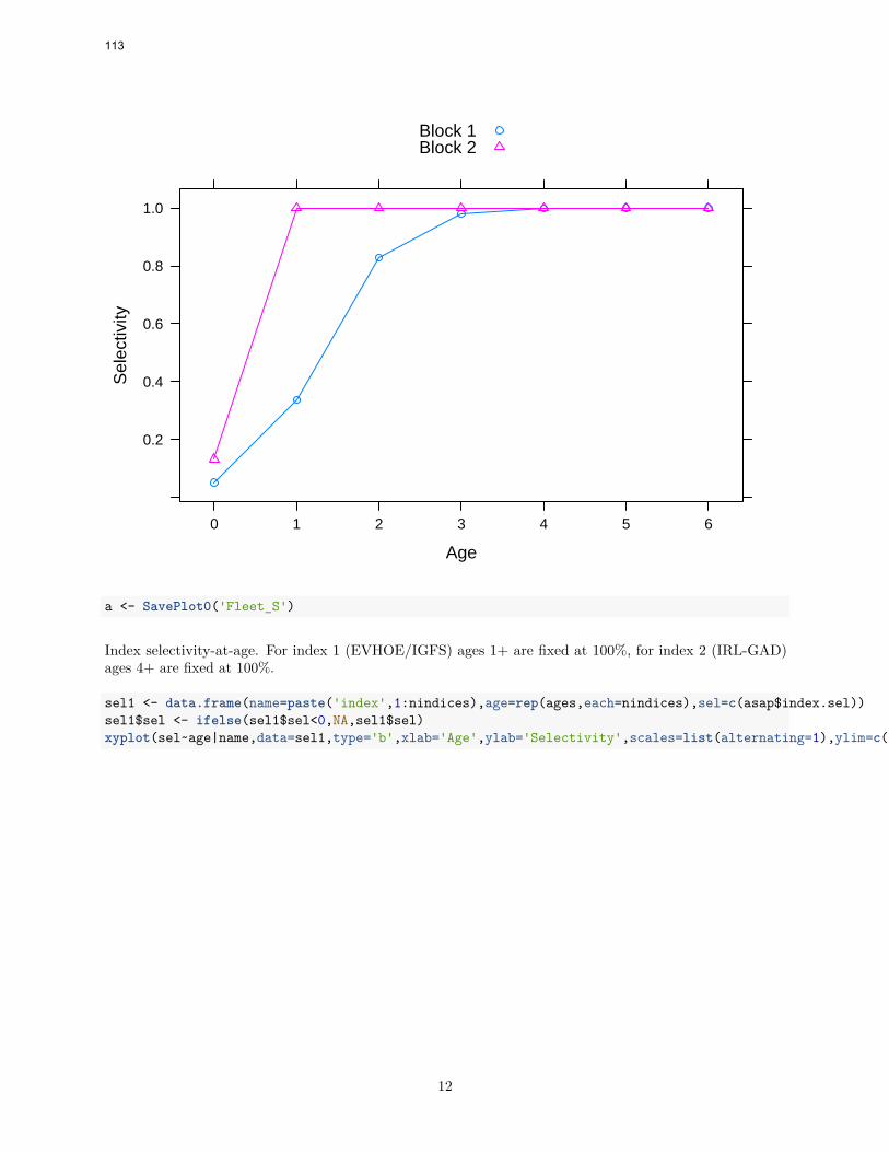
Age
Sel
ectiv
ity
0.2
0.4
0.6
0.8
1.0
0 1 2 3 4 5 6
Block 1Block 2
a <- SavePlot0('Fleet_S')
Index selectivity-at-age. For index 1 (EVHOE/IGFS) ages 1+ are fixed at 100%, for index 2 (IRL-GAD)ages 4+ are fixed at 100%.
sel1 <- data.frame(name=paste('index',1:nindices),age=rep(ages,each=nindices),sel=c(asap$index.sel))sel1$sel <- ifelse(sel1$sel<0,NA,sel1$sel)xyplot(sel~age|name,data=sel1,type='b',xlab='Age',ylab='Selectivity',scales=list(alternating=1),ylim=c(-.04,1.04))
12
113

Age
Sel
ectiv
ity
0.0
0.2
0.4
0.6
0.8
1.0
0 1 2 3 4 5 6
index 1
0 1 2 3 4 5 6
index 2
0 1 2 3 4 5 6
index 3
a <- SavePlot0('IndexSelectivity')
Save selectivity at age table for report
sel2 <- data.frame(ages,subset(sel,years==max(years))$values,t(asap$index.sel))names(sel2) <- c('Age','Catch',indices[1:nindices])for(i in 2:ncol(sel2)) sel2[,i] <- ifelse(sel2[,i]<0,NA,sel2[,i])write.csv(sel2,file.path(outdir,'whg7a_asap_sel.csv'),row.names=F)
Index q
ind3 <- NULLfor(i in 1:nindices){
ind3 <- rbind(ind3, data.frame(years=years[asap$index.year.counter[[i]]],name=indices[i],q=asap$q.indices[[i]]))}xyplot(q~years|name,data=ind3,type='b',scales=list(alternating=1))
13
114
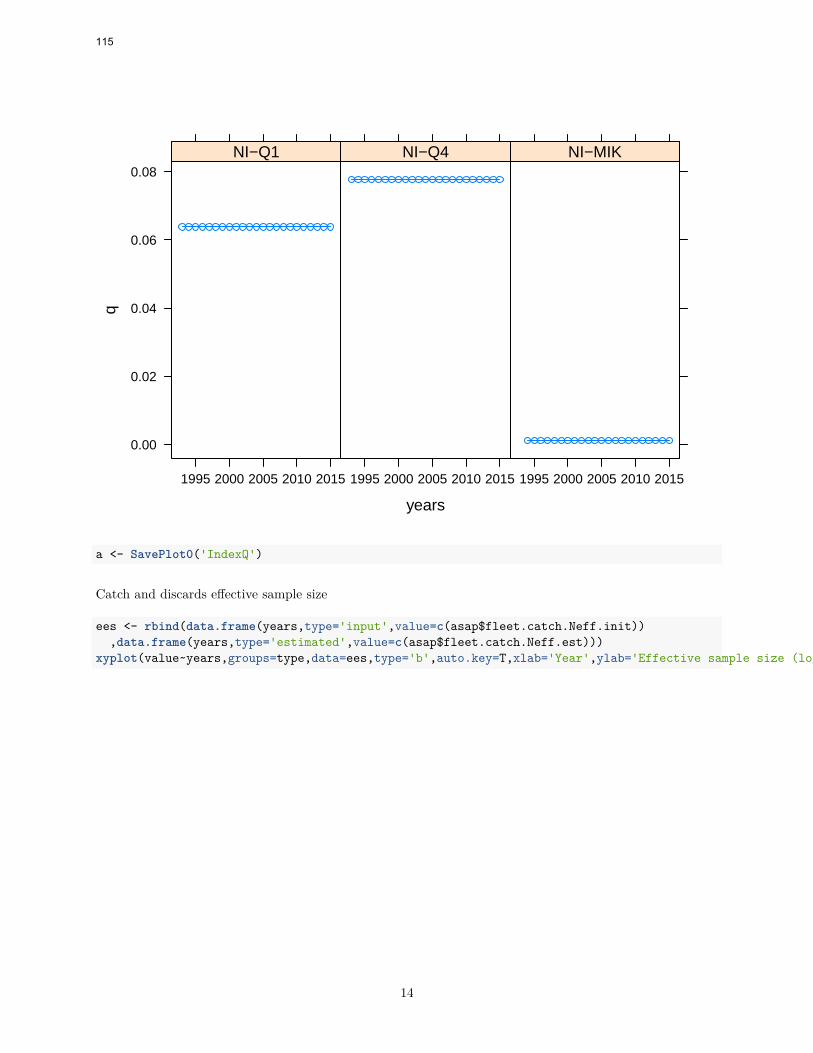
years
q
0.00
0.02
0.04
0.06
0.08
1995 2000 2005 2010 2015
NI−Q1
1995 2000 2005 2010 2015
NI−Q4
1995 2000 2005 2010 2015
NI−MIK
a <- SavePlot0('IndexQ')
Catch and discards effective sample size
ees <- rbind(data.frame(years,type='input',value=c(asap$fleet.catch.Neff.init)),data.frame(years,type='estimated',value=c(asap$fleet.catch.Neff.est)))
xyplot(value~years,groups=type,data=ees,type='b',auto.key=T,xlab='Year',ylab='Effective sample size (log scale)',scales=list(alternating=1,y=list(log=T)))
14
115
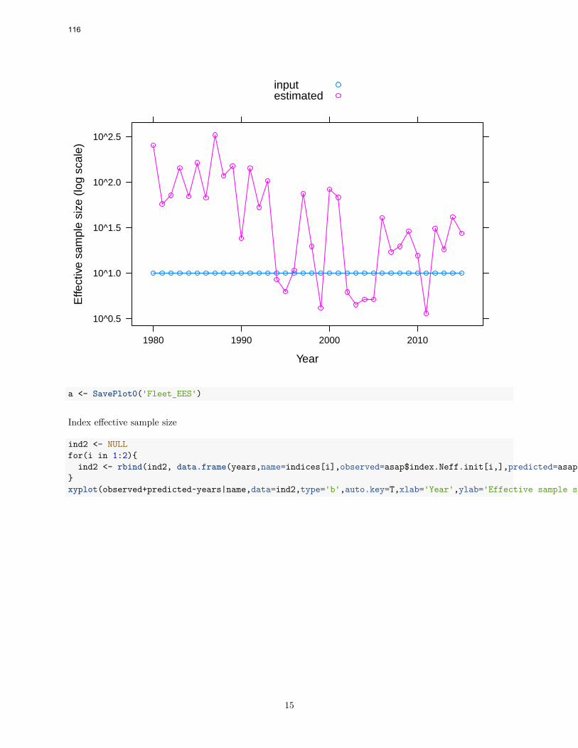
Year
Effe
ctiv
e sa
mpl
e si
ze (
log
scal
e)
10^0.5
10^1.0
10^1.5
10^2.0
10^2.5
1980 1990 2000 2010
inputestimated
a <- SavePlot0('Fleet_EES')
Index effective sample size
ind2 <- NULLfor(i in 1:2){
ind2 <- rbind(ind2, data.frame(years,name=indices[i],observed=asap$index.Neff.init[i,],predicted=asap$index.Neff.est[i,]))}xyplot(observed+predicted~years|name,data=ind2,type='b',auto.key=T,xlab='Year',ylab='Effective sample size',scales=list(alternating=1,y=list(log=T)))
15
116

Year
Effe
ctiv
e sa
mpl
e si
ze
10^1.0
10^1.5
10^2.0
10^2.5
10^3.0
1980 1990 2000 2010
NI−Q1
1980 1990 2000 2010
NI−Q4
observedpredicted
a <- SavePlot0('IndexEffSampSize')
Population numbers.
snaa <- asap$N.agesnaa.df <- stack(as.data.frame(snaa))snaa.df$year <- years# something wrong with cohorts i thinksnaa.df$cohort <- snaa.df$year - as.numeric(as.character(snaa.df$ind))-1key <- simpleKey(as.character(ages),space='right',title='age',cex.title=1)key$points$pch <- 1:nagesxyplot(log(values)~cohort,groups=factor(ind),data=snaa.df,type='b',key=key,pch=1:nages,scales=list(alternating=1),xlab='Cohort',ylab='Log stock numbers at age',cex=0.6)
16
117

Cohort
Log
stoc
k nu
mbe
rs a
t age
2
4
6
8
10
12
14
1980 1990 2000 2010
age0123456
a <- SavePlot0('StockNos')
The objective function. I think you want the value to be approximately evenly spread between the parameters
obj <- unlist(asap$like)[-1]par(las=1,mar=c(5,12,4,2))b <- barplot(obj,names=gsub('lk.','',names(obj)),horiz=T,xlab='Value')text(obj,b,ifelse(obj==0,0,''),pos=4)
17
118
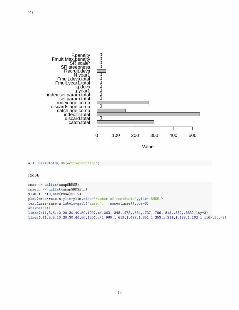
catch.totaldiscard.totalindex.fit.total
catch.age.compdiscards.age.comp
index.age.compsel.param.total
index.sel.param.totalq.year1q.devs
Fmult.year1.totalFmult.devs.total
N.year1Recruit.devs
SR.steepnessSR.scaler
Fmult.Max.penaltyF.penalty
Value
0 100 200 300 400 500
0
0
0000000
0000
a <- SavePlot0('ObjectiveFunction')
RMSE
rmse <- unlist(asap$RMSE)rmse.n <- unlist(asap$RMSE.n)ylim <- c(0,max(rmse)*1.2)plot(rmse~rmse.n,ylim=ylim,xlab='Number of residuals',ylab='RMSE')text(rmse~rmse.n,labels=gsub('rmse.','',names(rmse)),pos=3)abline(h=1)lines(c(1,3,5,10,20,30,40,50,100),c(.063,.348,.473,.634,.737,.786,.815,.832,.883),lty=3)lines(c(1,3,5,10,20,30,40,50,100),c(1.960,1.619,1.487,1.351,1.253,1.211,1.183,1.162,1.116),lty=3)
18
119

0 10 20 30 40 50 60 70
0.0
0.5
1.0
1.5
2.0
Number of residuals
RM
SE catch.tot
discard.tot
ind01
ind02
ind03ind.total
N.year1Fmult.year1Fmult.devs.total
recruit.devs
fleet.sel.paramsindex.sel.paramsq.year1q.devsSR.steepnessSR.scaler
a <- SavePlot0('RMSE')
Retrospective
par(mfrow=c(2,2))xlim <- range(years)ylim <- c(0,max(unlist(lapply(retro,function(x) x$catch.pred/1000))))plot(NA,xlim=xlim,ylim=ylim,xlab='Year',ylab='Kt',main='Catch')a <- lapply(retro,function(x) lines(as.numeric(colnames(x$catch.pred)),x$catch.pred/1000,col=x$col))ylim <- c(0,max(unlist(lapply(retro,function(x) x$SSB/1000))))plot(NA,xlim=xlim,ylim=ylim,xlab='Year',ylab='Kt',main='SSB')a <- lapply(retro,function(x) lines(as.numeric(colnames(x$catch.pred)),x$SSB/1000,col=x$col))ylim <- c(0,max(unlist(lapply(retro,function(x) x$F.report))))plot(NA,xlim=xlim,ylim=ylim,xlab='Year',ylab='F',main=paste0('Fbar ',paste(range(fbarage),collapse='-')))a <- lapply(retro,function(x) lines(as.numeric(colnames(x$catch.pred)),x$F.report,col=x$col))ylim <- c(0,max(unlist(lapply(retro,function(x) x$N.age[,1]/1000))))plot(NA,xlim=xlim,ylim=ylim,xlab='Year',ylab='Millions',main='Recruits age 0')a <- lapply(retro,function(x) lines(as.numeric(colnames(x$catch.pred)),x$N.age[,1]/1000,col=x$col))
19
120

1980 1990 2000 2010
0e+
002e
+10
4e+
10Catch
Year
Kt
1980 1990 2000 2010
0.0e
+00
8.0e
+12
SSB
Year
Kt
1980 1990 2000 2010
0.0
0.5
1.0
1.5
Fbar 1−3
Year
F
1980 1990 2000 2010
0e+
002e
+14
4e+
14Recruits age 0
Year
Mill
ions
a <- SavePlot0('Retrospective',6,6)
Retrospective, zoomed in
par(mfrow=c(2,2))xlim <- c(1995,2015)ylim <- c(0,3)plot(NA,xlim=xlim,ylim=ylim,xlab='Year',ylab='Kt',main='Catch')a <- lapply(retro,function(x) lines(as.numeric(colnames(x$catch.pred)),x$catch.pred/1000,col=x$col))ylim <- c(0,3)plot(NA,xlim=xlim,ylim=ylim,xlab='Year',ylab='Kt',main='SSB')a <- lapply(retro,function(x) lines(as.numeric(colnames(x$catch.pred)),x$SSB/1000,col=x$col))ylim <- c(0,max(unlist(lapply(retro,function(x) x$F.report))))plot(NA,xlim=xlim,ylim=ylim,xlab='Year',ylab='F',main=paste0('Fbar ',paste(range(fbarage),collapse='-')))a <- lapply(retro,function(x) lines(as.numeric(colnames(x$catch.pred)),x$F.report,col=x$col))ylim <- c(0,350)
20
121

plot(NA,xlim=xlim,ylim=ylim,xlab='Year',ylab='Millions',main='Recruits age 0')a <- lapply(retro,function(x) lines(as.numeric(colnames(x$catch.pred)),x$N.age[,1]/1000,col=x$col))
1995 2000 2005 2010 2015
0.0
1.0
2.0
3.0
Catch
Year
Kt
1995 2000 2005 2010 2015
0.0
1.0
2.0
3.0
SSB
Year
Kt
1995 2000 2005 2010 2015
0.0
0.5
1.0
1.5
Fbar 1−3
Year
F
1995 2000 2005 2010 2015
010
020
030
0
Recruits age 0
Year
Mill
ions
a <- SavePlot0('Retrospective1',6,6)
Organise the data for the tables
asap.std <- read.table(file.path(asapdir,'run-final.std'),header=T,fill=T)
#lan <- c(stock0@landings)#dis <- c(stock0@discards)catch <- c(asap$catch.obs)catch.pred <- c(asap$catch.pred) # asap predicted catch#catchInt <- c(landings(stf1)[,nyears+1]+discards(stf1)[,nyears+1]) # catch in intermediate year, assuming fsq#landInt <- c(landings(stf1)[,nyears+1])
21
122

ssb <- c(asap$SSB)#ssbInt <- c(ssb(stf1)[,nyears+1]) # ssb in intermediate year (1 jan)tsb <- c(apply(asap$N.age * asap$WAA.mats$WAA.ssb,1,sum))recr <- c(asap$N.age[,1])fbar <- c(asap$F.report)ssbSTD <- subset(asap.std,name=='SSB')$std # standard deviationrecrSTD <- subset(asap.std,name=='recruits')$std # standard deviationfbarSTD <- subset(asap.std,name=='Freport')$std # standard deviation
Summary plot
par(mfrow=c(2,2))
xlim <- range(years)+0:1ylim <- c(0,max(catch)/1000)plot(NA,xlim=xlim,ylim=ylim,xlab='Year',ylab='Kt',main='Catch')points(years,catch/1000)lines(years,catch.pred/1000)legend('topright',c('Observed','Predicted'),lty=c(NA,1),pch=c(1,NA),bty='n')#lines(years,lan/1000,lty=2)#points(max(years)+1,catchInt/1000)#points(max(years)+1,landInt/1000,pch=2)#legend('topright',c('Catch','Landings','Catch Fsq','Land Fsq'),lty=c(1,2,NA,NA),pch=c(NA,NA,1,2),bty='n',y.intersp=0.8)
ylim <- c(0,max(ssb+ssbSTD)/1000)plot(NA,xlim=xlim,ylim=ylim,xlab='Year',ylab='Kt',main='SSB')polygon(c(years,rev(years)),c((ssb-ssbSTD),rev((ssb+ssbSTD)))/1000,border=0,col='grey')lines(years,ssb/1000)lines(years,c(ssb(xsa+stock))/1000,col=2)legend('topright',c('asap','xsa'),lty=1,col=1:2,bty='n')#points(max(years)+1,ssbInt/1000)#legend('topleft',c('StDev',paste('1 jan',max(years)+1)),fill=c('grey',NA),border=NA,,pch=c(NA,1),bty='n')
ylim <- c(0,max(fbar+fbarSTD,fbar(xsa+stock)))plot(NA,xlim=xlim,ylim=ylim,xlab='Year',ylab='F',main=paste0('Fbar ',paste(range(fbarage),collapse='-')))polygon(c(years,rev(years)),c((fbar-fbarSTD),rev((fbar+fbarSTD))),border=0,col='grey')lines(years,fbar)lines(years,c(fbar(xsa+stock)),col=2)legend('topright',c('asap','xsa'),lty=1,col=1:2,bty='n')
#points(max(years)+1,fsq)#legend('bottomleft',c('StDev','Fsq'),pch=c(NA,1),fill=c('grey',NA),border=NA,bty='n')
ylim <- c(0,max(recr/1000))plot(NA,xlim=xlim,ylim=ylim,xlab='Year',ylab='Millions',main='Recruits age 0')polygon(c(years,rev(years)),c((recr-recrSTD),rev((recr+recrSTD)))/1000,border=0,col='grey')lines(years,recr/1000)lines(years,c([email protected][1,])/1000,col=2)legend('topright',c('asap','xsa'),lty=1,col=1:2,bty='n')
22
123

1980 1990 2000 2010
05
1015
20Catch
Year
Kt
ObservedPredicted
1980 1990 2000 2010
010
3050
SSB
Year
Kt
asapxsa
1980 1990 2000 2010
0.0
0.5
1.0
1.5
2.0
Fbar 1−3
Year
F
asapxsa
1980 1990 2000 2010
020
060
0Recruits age 0
Year
Mill
ions
asapxsa
#points(max(years)+1,GM/1000)#legend('topleft',c('StDev','GM'),pch=c(NA,1),fill=c('grey',NA),border=NA,bty='n')
a <- SavePlot0('Summary',6,6)
23
124

ICES WKIrish3 REPORT 2017 | 125
Annex 7: Whiting reference points
Whiting 7a MSY evaluationsColm Lordan
17 February 2017
The ICES approach to setting Reference Points
This Markdown document outlines the steps involved in estimating PA and MSY reference points for IrishSea whiting as part of the WKIRISH3 benchmark. The objective is to have a reproducible document thattransparently outlines the process, settings and decisions.
The ICES technical guidelines document establishes the procedures to be followed.
These have been developed based on the experiences and approach applied at WKMSYREF4 whichestimated PA reference points and Fmsy and MSY ranges for category 1 stocks in western waters andWKMSYREF3 which estimated Fmsy and MSY ranges for North Sea stocks.
For typical age-based assessments the preferred ICES approach used the EqSim methodology. This is availablefrom the developmental repository for the ‘msy package’ which is located on github, more specifically ongithub.com/ices-tools-prod/msy
To download the required packages for the very first time run the following code chunk by switching ‘eval =TRUE’.install.packages("devtools")install.packages("icesAdvice")install.packages("ggplot2")library(devtools)install.packages("FLCore", repo = "http://flr-project.org/R")install.packages("ggplotFL", repo = "http://flr-project.org/R")install_github("ices-tools-prod/msy")
knitr::opts_chunk$set(eval = TRUE, echo = TRUE, message = FALSE, warning = FALSE)
Load Packages
First we load the various packages needed to preform the analysis.library(ggplot2)library(ggplotFL)library(FLCore)library(msy)library(icesAdvice)library(knitr)
Load the data
Next we load the data. The current version of eqsim only takes FLStock objects as inputs. Note ‘eqsim’ willinternally use the landings and catch numbers at age provided in the FLStock object used as input to eqsimto calculate a discard ratio at age, which it then uses to split the long-term catch into landings and discards(at age).
1
126

Fix for zero weights
If there are a few zeros in the catch and stock weights and numbers that produces NaNs so this is a fix to fillthem in with a low value.load("L:/Data for ICESWG/2016/Benchmarks/WKIRISH/whgVIIa/Assessment/4_Outputs/whg7a_asap.Rdata")
[email protected] <- ifelse([email protected]==0,0.000001,[email protected])[email protected] <- ifelse([email protected]==0,0.000001,[email protected])[email protected] <- ifelse([email protected]==0,0.000001,[email protected])[email protected] <- ifelse([email protected]==0,0.000001,[email protected])[email protected] <- ifelse([email protected]==0,0.000001,[email protected])[email protected] <- ifelse([email protected]==0,0.000001,[email protected])[email protected] <- ifelse([email protected]==0,0.000001,[email protected])[email protected] <- ifelse([email protected]==0,0.000001,[email protected])
Stock Recruit summary
The first step in the process is to examine the stock and recruit pairs and decide on a Blim value. The defaultis approach is to choose the SSB value below which recruitment reduces with SSB, e.g. the change point of asegmented regression. However you should use the technical guidelines document to guide your expertdecision.
In the case of Irish Sea Whiting there is clear evidence of impaired recruitment at stock sizes below 10,000tbased on the S/R pairs from the assessment and that looks like and appropriate Blim. Various summarystatistics on the SSB estimates are provided in Table 1.# plotting SR relationshipssb <-as.data.frame(ssb(stock))ssb$var <- "SSB"rec <-as.data.frame(rec(stock))rec$var <- "Recruitment"sr <- data.frame(year=ssb$year, SSB=ssb$data, Recruitment=rec$data)ggplot(sr, aes(SSB, Recruitment)) + geom_point() +
geom_text(aes(label=year), hjust=-0.1) + theme_bw() +xlim(0, max(sr$SSB)*1.05)
2
127

1980
19811982
1983
1984
1985
1986
1987 1988
1989
1990
1991
199219931994
1995
199619971998
1999
2000
2001
2002200320042005
2006
20072008
20092010
2011
2012
20132014
2015
250000
500000
750000
0 10000 20000 30000 40000
SSB
Rec
ruitm
ent
Figure 1: Stock and recruitment pairs for Irish Sea whiting by year.stock.cur <- ssb$data[ssb$year==stock@range[5]]stock.loss <- min(ssb$data)stock.50 <- as.numeric(quantile(ssb$data,0.5))stock.75 <- as.numeric(quantile(ssb$data,0.75))stock.max <- max(ssb$data)
An example fit of a Beverton and Holt stock and recruitment model is shown in Figure 2 below. The functionalform of the relationship is quite different to the fitted model but despite that the residuals by year show areasonable fit. There is no indication of autocorrelation in residuals as the slope in panel 3 is pretty muchhorizontal. The clumped nature of the stock-recruit pairs with lots of recruitments observed at low stock sizeis particularly obvious in the residuals by SSB plot (panel 4). The Q-Q plot and the residuals by recruitslook relatively good.srbh <- fmle(as.FLSR(stock, model="bevholt"), method="L-BFGS-B", lower=c(1e-6, 1e-6), upper=c(max(rec(stock)) * 3, Inf))
## iter 10 value -24.250382## final value -24.487859## convergedplot(srbh)
3
128

0
250000
500000
750000
0 10000 20000 30000 40000
SSB
Rec
ruits
−0.4
0.0
0.4
1980 1990 2000 2010
Year
Res
idua
ls
−0.4
0.0
0.4
−0.4 0.0 0.4
Residualst
Res
idua
lst+
1
−1.2
−0.8
−0.4
0.0
0.4
0 10000 20000 30000 40000
SSB
Res
idua
ls
−0.4
0.0
0.4
−2 −1 0 1 2
Theoretical
Sam
ple
−0.4
0.0
0.4
1e+05 2e+05 3e+05 4e+05 5e+05
Recruits^
Res
idua
ls
Figure 2: Example of fit with Beverton and Holt Stock and recruitment model. Panels: (1) stock-recruit data,fitted model in this case a Beverton and Holt and lowess smoother, (2) residuals by year, (3) lag 1-correlatedresiduals, (4) residuals by SSB, (5) residuals qqplot and (6) residuals by fitted values. Blue lines are loewesssmoothers, to better visualize trends in the data shown.
Table 1. Summary of SSB values
SSB ref value SSB EstimateTerminal SSB 852tMin observed 531t50th Percentile 2622t75th Percentile 15380tMax observed 43330t
Estimating the breakpoint stochastically
The msy package can be use to estimate the break-point stochastically. In the case of Irish Sea whiting thebreak-point is very low because there are many observations of low recruitment at low stock size and theestimated break-point is not considered a good candidate for Blim. Figure 3 below gives the estimates of thestochastic breakpoints.fit <- eqsr_fit(stock, nsamp = 1000, models = "Segreg")boxplot(fit$sr.sto$b.b, main="Stochastic Breakpoint estimates")
4
129

2000
3000
4000
5000
6000
Stochastic Breakpoint estimates
med.bp <- median(fit$sr.sto$b.b)
Figure 3: Box plot of break-point estimates for Irish Sea whiting.
The median estimate of the break-point is 3489t.
Uncertainty parameters
In the ICES approach Bpa is the estimated SSB which ensures that the true SSB has less than 5% probabilityof being below Blim. In practice this requires an estimate of sigma, the standard deviation of ln(SSB) at thestart of the year following the terminal year of the assessment.
In the absence of an estimate the default is 0.2.
In the case of the ASAP assessments you can take the Fcv and SSBcv from the final year of the assessmentmodel.Fcv <- 0.303757SSBcv <- 0.297147Blim <- 10000Bpa <- round(Bpa(Blim, SSBcv)/100, 0)*100Fphi <- 0.423
For Irish Sea whiting Blim is set at 10000 t and Bpa is estimated at 16300 t.
5
130

Estimating Fmsy using multiple Stock and Recruit models
The base Eqsim analysis largely uses default settings for the input parameters: Selection pattern is thedefault 10 year range. Biological parameters is the default of 10 years (although this is something the WGshould monitor as trends maybe developing) The scan sequence is fairly granular to have more consistentinterpolations. The uncertainties are as specified above.
In the case of the Irish Sea whiting we have a priori ruled out the segmented regression alone as a S/Rrelationship. The software allows for uncertainty in the stock-recruitment model is taken into account byapplying model averaging using smooth AIC weights (Buckland et al. 1997). Here we use the three standardmodel and also specify a segmented regression with a fixed break-point at Blim.
The fit of the mixed model to the observations looks good. The Beverton and Holt gets most of the weight.The two segmented regression options get no weight.
The issue here is that the F0.5 - the 5% probability of dropping below Blim is pretty much the same andFmsy. This is potentially not a problem and F0.5 becomes the upper bound of the Fmsy range.setup <- list(data = stock,bio.years = c(2006, 2015),bio.const = FALSE,sel.years = c(2006, 2015),sel.const = FALSE,Fscan = seq(0, 1.5, by=0.025),Fcv = Fcv, Fphi = Fphi,Blim = Blim,Btrigger = 0,Bpa = Bpa(Blim, SSBcv),extreme.trim=c(0.05,0.95))
FixedBlim<-function (ab, ssb){log(ifelse(ssb >= Blim, ab$a * Blim, ab$a * ssb))}
res <- within(setup,{fit <- eqsr_fit(data, nsamp = 1000, models = c("Ricker", "Bevholt", "FixedBlim",
"Segreg"))sim <- eqsim_run(fit, bio.years = bio.years, bio.const = bio.const,sel.years = sel.years, sel.const = sel.const, Fscan = Fscan,Fcv = Fcv, Fphi = Fphi, Blim = Blim, Bpa = Bpa, Btrigger = Btrigger,extreme.trim = extreme.trim, verbose = FALSE)})
Fmsy is initially calculated as the F that maximizes median long-term yield in stochastic simulation underconstant F exploitation (i.e. without MSY Btrigger). EqSim internally uses the landings and catch numbersat age provided in the FLStock object used as input to calculate a discard ratio at age, which it then uses tosplit the long-term catch into landings and discards (at age). The choice of yield is a choice for policy and,following discussions with clients, ICES defines yield to be catch above the minimum catch/conservationsize. When the selection pattern corresponding to this cannot be estimated, ICES uses the recent landingsselection to define yield. In the case of Irish Sea whithing where discarding accounts for more than 95%of the catch the logic of defining Fmsy based on the sparse landings at age data in recent years is open toquestion. Nevertheless we estimate Fmsy here according to the guidelines although there is a strong caveatthat it is based on current retention practices and selection patterns which are not well estimated.
In figure 4 below we see that the median estimate if Fmsy is 0.22 which is expected to generate medianlandings of around 1600t. The Fmsy value is also very close to F(5%). Following the ICES procedure we
6
131

need to calculate the Fpa because if Fmsy is greater than Fpa then we reduce Fmsy to Fpa.eqsim_plot_range(res$sim, type="median")
0.0 0.5 1.0 1.5
050
010
0015
00
Total catch F
Med
ian
land
ings
F(msy)
lower = 0.15median = 0.21upper = 0.296
F(5%)
lower = 0.152estimate = 0.217upper = 0.294
Figure 4: Yield curve and FMSY upper and lower ranges (vertical blue lines) and Flim upper and lowerranges (vertical green lines) for the mixed stock recruit model. Fmsy median point estimates and upper andlower bound are given (bottom right).
The Median SSB for the Fmsy range is shown in Figure 5 below. The value for median SSB corresponding tothe lower and upper Fmsy bounds are also shown on the plot. For some reason the code returns an NA forthe median SSB corresponding to the median Fmsy.eqsim_plot_range(res$sim, type="ssb")
7
132

0.0 0.5 1.0 1.5
010
000
2000
030
000
Total catch F
Med
ian
SS
B
F(msy)
lower = 20480median = NAupper = 12252
Figure 5: Median SSB curve over a range of target F values. Blue line correspond to the FMSY range.
Figure 6 shows the Eqsim summary of various recruitment models using the default “Buckland” method(Ricker, Beverton and Holt, segmented regression and fixed break-point). This plot indicates that the final SRmodel is driven by the Beverton and Holt and the two segmented regression options don’t fit well to the data.eqsr_plot(res$fit,ggPlot=FALSE)
8
133

0 10000 20000 30000 40000
040
0000
8000
0012
0000
0Predictive distribution of recruitment
for
SSB ('000 t)
Rec
ruits
Ricker 0.04
Bevholt 0.96
FixedBlim NA
Segreg NA
Figure 6: Eqsim summary of recruitment models using the default “Buckland” method (Ricker, Bevertonand Holt and segmented regression). The final model is shown in yellow, the Ricker is shown as black, theBeverton an Holt is the black dashed line, estimated segmented regression is the black dash and dot line andthe fixed break-point at 10,000t is the black dotted line. The various weights are also indicated on the plot.
The Eqsim summary plots in Figure 7b and c highlight the fact that F and catch in the past has been wellabove the sustainable ranges estimated. Figure 5d indicates that the risk to Blim overlaps with the Fmsyprobability at a fairly low F values.eqsim_plot(res$sim, catch = TRUE)
9
134

0.0 0.5 1.0 1.5
0e+00
2e+05
4e+05
6e+05
8e+05
1e+06
F05
F bar
Rec
ruitm
ent
a) Recruits
0.0 0.5 1.0 1.5
0
10000
20000
30000
40000
50000
F05
F bar
Spa
wni
ng s
tock
bio
mas
s
b) Spawning stock biomass
0.0 0.5 1.0 1.5
0
5000
10000
15000
20000
25000
F05
Cat
ch
c) Catch
med
ian
Fm
sym
ean
Fm
sy
0.0 0.5 1.0 1.5
0.0
0.2
0.4
0.6
0.8
1.0
Pro
b M
SY,
SS
B<
Bpa
or
Blim
d) Prob MSY and Risk to SSB
SSB<BlimSSB<BpaProb of cFmsyProb of lFmsy
5%
Figure 7: Eqsim summary plot. Panels a-c: historic values (dots) median (solid black) and 90% intervals(dotted black) recruitment, SSB and landings for exploitation at fixed values of F. Panel c also shows meanlandings (red solid line). Panel d shows the probability of SSB less than Blim (red), SSB less than BPA(green) and the cumulative distribution of FMSY based on yield as landings (brown) and catch (cyan).
Carmen said The same output can be obtained from the slot refs_interval. In this case, the value to useis the one labelled FmsyMedianL, which should coincide with the one obtained in Refs2 (minor differencesbetween both values could occur because the interpolation has been done differently for the 2 slots. but thedifferences should, if they exist at all, be very minor. . . otherwise it d be a signal that something is wrong inthe EqSim code).
Table 2. Output values from the Eqsim analysis.kable(t(res$sim$Refs2), digits=c(3,3,0,0,0,0))
catF lanF catch landings catB lanBF05 0.217 NA 4144 NA 16114 NAF10 0.243 NA 4300 NA 14706 NAF50 0.356 NA 4548 NA 9990 NAmedianMSY NA 0.210 NA 1669 NA 16511meanMSY 0.350 0.225 4550 1666 10189 15673Medlower NA 0.150 NA 1584 NA 20480Meanlower NA 0.152 NA 1709 NA NAMedupper NA 0.296 NA 1584 NA 12252Meanupper NA 0.297 NA 1705 NA NA
10
135
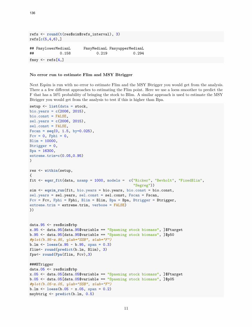
refs <- round(t(res$sim$refs_interval), 3)refs[c(5,4,6),]
## FmsylowerMedianL FmsyMedianL FmsyupperMedianL## 0.158 0.219 0.294fmsy <- refs[4,]
No error run to estimate Flim and MSY Btrigger
Next Eqsim is run with no error to estimate Flim and the MSY Btrigger you would get from the analysis.There a a few different approaches to estimating the Flim point. Here we use a loess smoother to predict theF that has a 50% probability of bringing the stock to Blim. A similar approach is used to estimate the MSYBtrigger you would get from the analysis to test if this is higher than Bpa.setup <- list(data = stock,bio.years = c(2006, 2015),bio.const = FALSE,sel.years = c(2006, 2015),sel.const = FALSE,Fscan = seq(0, 1.5, by=0.025),Fcv = 0, Fphi = 0,Blim = 10000,Btrigger = 0,Bpa = 16300,extreme.trim=c(0.05,0.95))
res <- within(setup,{fit <- eqsr_fit(data, nsamp = 1000, models = c("Ricker", "Bevholt", "FixedBlim",
"Segreg"))sim <- eqsim_run(fit, bio.years = bio.years, bio.const = bio.const,sel.years = sel.years, sel.const = sel.const, Fscan = Fscan,Fcv = Fcv, Fphi = Fphi, Blim = Blim, Bpa = Bpa, Btrigger = Btrigger,extreme.trim = extreme.trim, verbose = FALSE)})
data.95 <- res$sim$rbpx.95 <- data.95[data.95$variable == "Spawning stock biomass", ]$Ftargetb.95 <- data.95[data.95$variable == "Spawning stock biomass", ]$p50#plot(b.95~x.95, ylab="SSB", xlab="F")b.lm <- loess(x.95 ~ b.95, span = 0.3)flim<- round(predict(b.lm, Blim), 3)fpa<- round(Fpa(flim, Fcv),3)
###BTriggerdata.05 <- res$sim$rbpx.05 <- data.05[data.05$variable == "Spawning stock biomass", ]$Ftargetb.05 <- data.05[data.05$variable == "Spawning stock biomass", ]$p05#plot(b.05~x.05, ylab="SSB", xlab="F")b.lm <- loess(b.05 ~ x.05, span = 0.2)msybtrig <- predict(b.lm, 0.5)
11
136

Running the code with no error gives an estimate of Flim = 0.371, and estimate of Fpa = 0.225, and MSYBtrigger of 4281t.
In this case the Fmsy estimate 0.219 very close to Fpa 0.225 so the lower of the two values should be used asfmsy.fmsy <- ifelse(fmsy>fpa, fpa, fmsy)
Evaluate the ICES MSY Advice Rule
The next step is to evaluate the ICES advice rune via the stochastic simulation with these values of FMSYand MSY Btrigger. If the Fmsy is less than the F5% in this run the the Fmsy stays the same if it is greaterthan Fmsy is reduced to F5%.
So EqSim is run again this time including the selected MSY Btrigger value and error.setup <- list(data = stock,bio.years = c(2006, 2015),bio.const = FALSE,sel.years = c(2006, 2015),sel.const = FALSE,Fscan = seq(0, 1.5, by=0.025),Fcv = 0.303757, Fphi = 0.423, #in the absence of this use WKMSYREF4 defaults
#Fcv=0.212, Fphi=0.423Blim = 10000,Btrigger = 16300,Bpa = 16300,extreme.trim=c(0.05,0.95))
res <- within(setup,{fit <- eqsr_fit(data, nsamp = 1000, models = c("Ricker", "Bevholt", "FixedBlim",
"Segreg"))sim <- eqsim_run(fit, bio.years = bio.years, bio.const = bio.const,sel.years = sel.years, sel.const = sel.const, Fscan = Fscan,Fcv = Fcv, Fphi = Fphi, Blim = Blim, Bpa = Bpa,extreme.trim = extreme.trim, verbose = FALSE)})
knitr::kable(t(res$sim$Refs2), digits=c(2,2,0,0,0,0))
catF lanF catch landings catB lanBF05 0.22 NA 4114 NA 16246 NAF10 0.24 NA 4274 NA 14803 NAF50 0.36 NA 4537 NA 10010 NAmedianMSY NA 0.23 NA 1672 NA 15628meanMSY 0.35 0.22 4538 1670 10272 15733Medlower NA 0.15 NA 1590 NA 20181Meanlower NA 0.15 NA 1708 NA NAMedupper NA 0.30 NA 1590 NA 12328Meanupper NA 0.30 NA 1704 NA NA
12
137

refs <- round(t(res$sim$refs_interval), 3)refs[c(5,4,6),]
## FmsylowerMedianL FmsyMedianL FmsyupperMedianL## 0.158 0.226 0.294
If the FMSY calculated above is less than the EqSim output Fp.05 (F that gives 5% probability of SSB lessthan Blim), then FMSY stays unchanged. In this case Fmsy = 0.219 is very close to the Fp.05 =0.226 butthe lower of the two becomes the final choice of FMSY.fmsy <- ifelse(fmsy>refs[4,], refs[4,], fmsy)
Retrospective analysis
This code does a retrospective analysis. It takes a long time to run so only run it when you need to.
The objective of the retrospective analysis is to investigate how stable the Fmsy estimate has been over timeusing the same input data but with a moving window for biological data and selection. Because the approachis to optimise the Fmsy on landings and the F is partioned between landings and discards based on numbersin the catch it is useful to see that the Fmsy is relatively stable over time.
The Fmsy for Irish Sea whiting shows a slightly declining trend over time (Figure 8). The distribution Fmsyestimate look to be very skewed with median estimates close to or at the lower bound in some years. Therange also seems to be narrower towards the end of the time serise.out <- NULLsetup$Fscan <- seq(0, 1.5, by=0.05)for(y in 2006:2015){
setup$bio.years <- c(y-10,y)setup$sel.years <- c(y-10,y)fit <- eqsr_fit(trim(setup$data, year=stock@range[4]:y), nsamp=1000,
models=c("Ricker", "Segreg", "Bevholt", "FixedBlim"))sim <- with(setup, eqsim_run(fit, bio.years = bio.years, bio.const = bio.const,sel.years = sel.years, sel.const = sel.const, Fscan = Fscan,Fcv = Fcv, Fphi = Fphi, Blim = Blim, Bpa = Bpa,extreme.trim = extreme.trim, verbose = FALSE))
out0 <- data.frame(y,Fmsy05 = with(subset(sim$p,variable=='pFmsyLandings'),
Ftarget[which.min(abs(value-0.05))]),Fmsy95 = with(subset(sim$p,variable=='pFmsyLandings'),
Ftarget[which.min(abs(value-0.95))]),FmsyMed = sim$Refs2[2,4],FmsyMean = sim$Refs2[2,5]
)out <- rbind(out,out0)
}
write.csv(out,"L:/Data for ICESWG/2016/Benchmarks/WKIRISH/whgVIIa/Assessment/4_Outputs/out.csv",row.names = FALSE)
out <- read.csv("L:/Data for ICESWG/2016/Benchmarks/WKIRISH/whgVIIa/Assessment/4_Outputs/out.csv")
par(mar=c(4.5,4,.5,.5))
13
138

plot(out$y,out$FmsyMed,type='b',ylim=c(0,0.7),xlab='Year', ylab='Fmsy')lines(out$y,out$Fmsy05-out$FmsyMed+out$FmsyMean,lty=3)lines(out$y,out$Fmsy95-out$FmsyMed+out$FmsyMean,lty=3)legend('bottomright',c('FmsyMedian','5% and 95%'),lty=c(1,3),pch=c(1,NA),bty='n',inset=0.02)
2006 2008 2010 2012 2014
0.0
0.1
0.2
0.3
0.4
0.5
0.6
0.7
Year
Fm
sy
FmsyMedian5% and 95%
Figure 8: Retrospective analysis using a 10 year moving window of biological parameters and selection toestimate Fmsy and the 95% confidence intervals (broken lines).
Table 2. Summary of reference ploints
Reference point Value Technical basisMSY Btrigger 16300 t BpaFMSY 0.22 Median point estimates of EqSim with combined SRBlim 10000 t Below 10,000 t recruitment is impairedBpa 16300 t Blim combined with the assessment errorFlim 0.37 F with 50% probability of SSB less than BlimFpa 0.22 Flim combined with the assessment error
rps <- FLPar(Catch=NA, Rec=NA, SSB=Blim, Harvest=fmsy)rps2 <- FLPar(Catch=NA, Rec=NA, SSB=16000, Harvest=0.4)plot(stock, rps) + theme_bw()
14
139

Catch
Harvest
Rec
SS
B
1980 1990 2000 2010
0
5000
10000
15000
20000
0.0
0.5
1.0
1.5
0
250000
500000
750000
0
10000
20000
30000
40000
Figure 9: Stock summary plot with Blim and Fmsy shown as blue lines.
Session information
sessionInfo()
## R version 3.3.2 (2016-10-31)## Platform: i386-w64-mingw32/i386 (32-bit)## Running under: Windows Server 2008 R2 x64 (build 7601) Service Pack 1#### locale:## [1] LC_COLLATE=English_Ireland.1252 LC_CTYPE=English_Ireland.1252## [3] LC_MONETARY=English_Ireland.1252 LC_NUMERIC=C## [5] LC_TIME=English_Ireland.1252#### attached base packages:## [1] stats graphics grDevices utils datasets methods base#### other attached packages:## [1] knitr_1.15.1 icesAdvice_1.2-0 msy_0.1.18## [4] ggplotFL_2.5.9.9000 FLCore_2.6.0.20170214 lattice_0.20-34## [7] MASS_7.3-45 ggplot2_2.2.1#### loaded via a namespace (and not attached):## [1] Rcpp_0.12.9 magrittr_1.5 munsell_0.4.3 colorspace_1.3-2## [5] highr_0.6 stringr_1.1.0 plyr_1.8.4 tools_3.3.2
15
140

## [9] grid_3.3.2 gtable_0.2.0 htmltools_0.3.5 yaml_2.1.14## [13] lazyeval_0.2.0 rprojroot_1.2 digest_0.6.12 assertthat_0.1## [17] tibble_1.2 Matrix_1.2-7.1 gridExtra_2.2.1 reshape2_1.4.2## [21] evaluate_0.10 rmarkdown_1.3 labeling_0.3 stringi_1.1.2## [25] scales_0.4.1 backports_1.0.5 stats4_3.3.2
16
141

142 | ICES WKIrish3 REPORT 2017
Annex 8: Cod reference points
Cod 7a MSY evaluationsWKIrish3Sys.date()
R Markdown To Look at various eqsim runs
First load librarys and data.library(FLCore)
## Warning: package 'FLCore' was built under R version 3.3.2library(msy)library(dplyr)
## Warning: package 'dplyr' was built under R version 3.3.2library(icesAdvice)
## Warning: package 'icesAdvice' was built under R version 3.3.2#setwd("C:/Users/User1/Documents/")load("~/Cod7a_asap.Rdata")
1
143

SR summary
1968
1969
1970
1971
1972
1973
1974
1975
19761977
1978
1979
1980
1981
1982
19831984
1985
1986
1987
19881989
1990
1991
1992
1993
19941995
1996
1997
1998
1999
20002001
20022003
20042005200620072008
200920102011
20122013
2014
2015
0e+00
5e+04
1e+05
0 5000 10000 15000 20000
SSB
Rec
ruitm
ent
Table 1. Summary of values for SSB
SSB ref value SSB EstimateTerminal SSB 6913tMin observed 845t50th Percentile 7178t75th Percentile 13076tMax observed 20357t
There have been several TCMs introduced and changes in mesh size for some fleets over time.
fix for zero weights
[email protected] <- ifelse([email protected]==0,0.001,[email protected])[email protected] <- ifelse([email protected]==0,0.001,[email protected])[email protected] <- ifelse([email protected]==0,0.001,[email protected])[email protected] <- ifelse([email protected]==0,0.001,[email protected])[email protected] <- ifelse([email protected]==0,0.001,[email protected])[email protected] <- ifelse([email protected]==0,0.001,[email protected])stock@discards<-stock@catch-stock@landings
Stock recruitment fitted by ‘segmented regression’
2
144
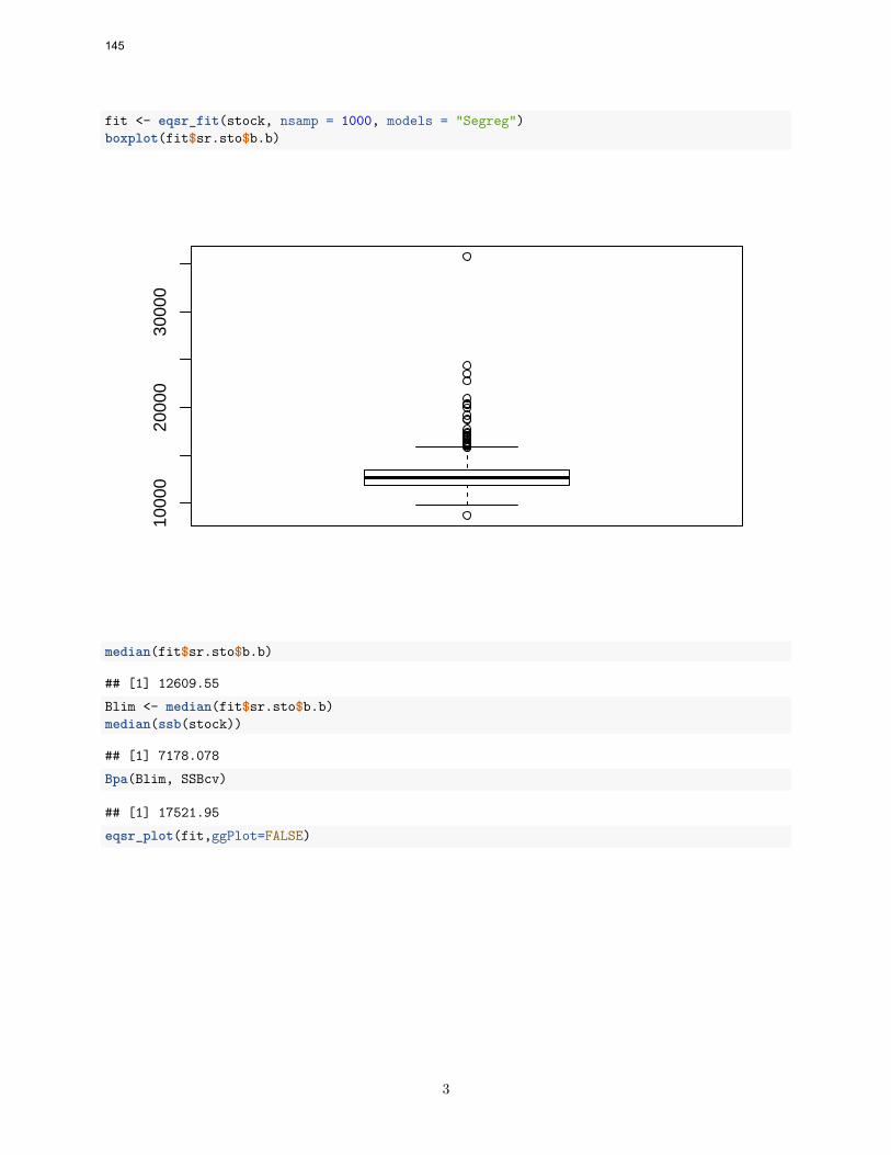
fit <- eqsr_fit(stock, nsamp = 1000, models = "Segreg")boxplot(fit$sr.sto$b.b)
1000
020
000
3000
0
median(fit$sr.sto$b.b)
## [1] 12609.55Blim <- median(fit$sr.sto$b.b)median(ssb(stock))
## [1] 7178.078Bpa(Blim, SSBcv)
## [1] 17521.95eqsr_plot(fit,ggPlot=FALSE)
3
145
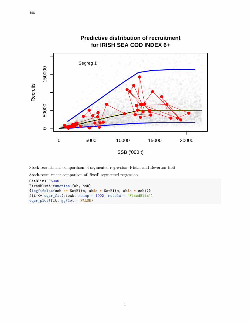
0 5000 10000 15000 20000
050
000
1500
00Predictive distribution of recruitment
for IRISH SEA COD INDEX 6+
SSB ('000 t)
Rec
ruits
Segreg 1
Stock-recruitment comparrison of segmented regression, Ricker and Beverton-Holt
Stock-recruitment comparison of ‘fixed’ segmented regressionSetBlim<- 6000FixedBlim<-function (ab, ssb){log(ifelse(ssb >= SetBlim, ab$a * SetBlim, ab$a * ssb))}fit <- eqsr_fit(stock, nsamp = 1000, models = "FixedBlim")eqsr_plot(fit, ggPlot = FALSE)
4
146
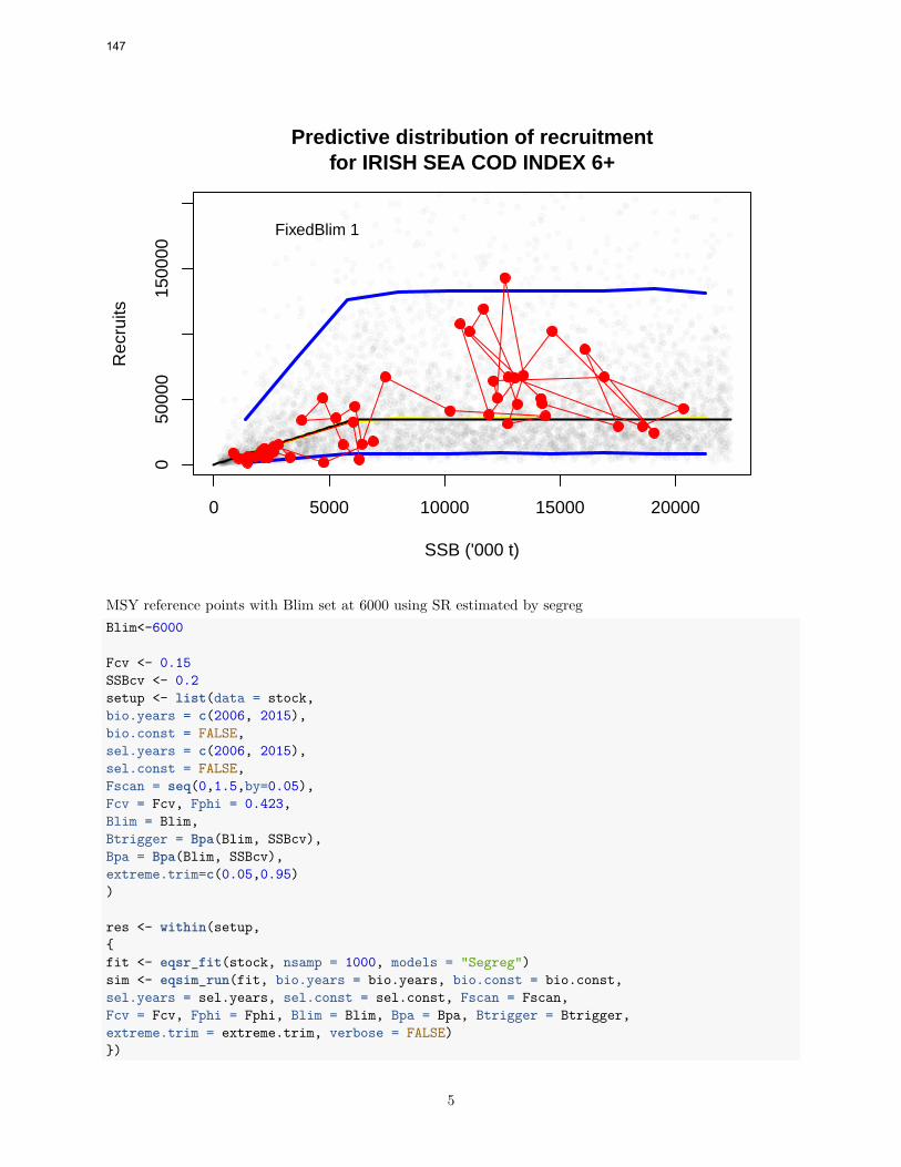
0 5000 10000 15000 20000
050
000
1500
00Predictive distribution of recruitment
for IRISH SEA COD INDEX 6+
SSB ('000 t)
Rec
ruits
FixedBlim 1
MSY reference points with Blim set at 6000 using SR estimated by segregBlim<-6000
Fcv <- 0.15SSBcv <- 0.2setup <- list(data = stock,bio.years = c(2006, 2015),bio.const = FALSE,sel.years = c(2006, 2015),sel.const = FALSE,Fscan = seq(0,1.5,by=0.05),Fcv = Fcv, Fphi = 0.423,Blim = Blim,Btrigger = Bpa(Blim, SSBcv),Bpa = Bpa(Blim, SSBcv),extreme.trim=c(0.05,0.95))
res <- within(setup,{fit <- eqsr_fit(stock, nsamp = 1000, models = "Segreg")sim <- eqsim_run(fit, bio.years = bio.years, bio.const = bio.const,sel.years = sel.years, sel.const = sel.const, Fscan = Fscan,Fcv = Fcv, Fphi = Fphi, Blim = Blim, Bpa = Bpa, Btrigger = Btrigger,extreme.trim = extreme.trim, verbose = FALSE)})
5
147

knitr::kable(t(res$sim$Refs2), digits=c(2,2,0,0,0,0))
catF lanF catch landings catB lanBF05 1.07 NA 8105 NA 12239 NAF10 1.14 NA 7425 NA 10382 NAF50 NA NA NA NA NA NAmedianMSY NA 0.60 NA 6780 NA 32717meanMSY 0.75 0.60 9686 6780 24071 32983Medlower NA 0.41 NA 6441 NA 52202Meanlower NA 0.42 NA 6910 NA NAMedupper NA 0.83 NA 6444 NA 20487Meanupper NA 0.85 NA 6909 NA NA
eqsim_plot_range(res$sim, type="median")
0.0 0.5 1.0 1.5
010
0030
0050
0070
00
Total catch F
Med
ian
land
ings
F(msy)
lower = 0.407median = 0.604upper = 0.83
F(5%)
lower = 0.212estimate = 1.068upper = 1.104
eqsim_plot_range(res$sim, type="ssb")
6
148

0.0 0.5 1.0 1.5
050
000
1000
0015
0000
Total catch F
Med
ian
SS
B
F(msy)
lower = 52202median = NAupper = 20487
#eqsr_plot(res$fit,ggPlot=FALSE)
#eqsim_plot2(res$sim, ymax.multiplier = 1.1, catch = FALSE) # note I modify the eqsim_plot function
No error run to estimate Flim and MSY Btrigger with fixed Blim from SegReg For the record we run Eqsimwith no error to estimate Flim and the MSY Btrigger you would get from the analysis to test if this is higherthan Bpa.setup <- list(data = stock,bio.years = c(2006, 2015),bio.const = FALSE,sel.years = c(2006, 2015),sel.const = FALSE,Fscan = seq(0,1.5,by=0.05),Fcv = 0.0, Fphi = 0.0,Blim = Blim,Btrigger = Bpa(Blim, SSBcv),Bpa = Bpa(Blim, SSBcv),extreme.trim=c(0.05,0.95))
res <- within(setup,{fit <- eqsr_fit(data, nsamp = 1000, models = "FixedBlim")sim <- eqsim_run(fit, bio.years = bio.years, bio.const = bio.const,sel.years = sel.years, sel.const = sel.const, Fscan = Fscan,
7
149

Fcv = Fcv, Fphi = Fphi, Blim = Blim, Bpa = Bpa,extreme.trim = extreme.trim, verbose = FALSE)})
knitr::kable(t(res$sim$Refs2), digits=c(2,2,0,0,0,0))
catF lanF catch landings catB lanBF05 0.97 NA 6892 NA 11765 NAF10 1.03 NA 6775 NA 10482 NAF50 1.31 NA 5376 NA 5997 NAmedianMSY NA 0.60 NA 4831 NA 23876meanMSY 0.80 0.60 7025 4830 15842 24074Medlower NA 0.41 NA 4593 NA 38207Meanlower NA 0.42 NA 5032 NA NAMedupper NA 0.88 NA 4590 NA 13552Meanupper NA 0.92 NA 5031 NA NA
eqsim_plot_range(res$sim, type="median")
0.0 0.5 1.0 1.5
010
0020
0030
0040
0050
00
Total catch F
Med
ian
land
ings
F(msy)
lower = 0.408median = 0.604upper = 0.884
F(5%)
lower = 0.318estimate = 0.966upper = 1.062
eqsim_plot_range(res$sim, type="ssb")
8
150
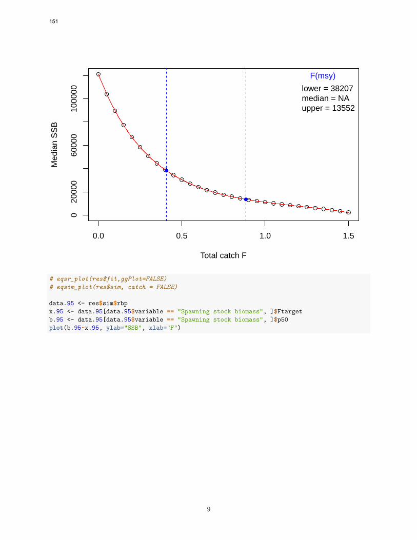
0.0 0.5 1.0 1.5
020
000
6000
010
0000
Total catch F
Med
ian
SS
B
F(msy)
lower = 38207median = NAupper = 13552
# eqsr_plot(res$fit,ggPlot=FALSE)# eqsim_plot(res$sim, catch = FALSE)
data.95 <- res$sim$rbpx.95 <- data.95[data.95$variable == "Spawning stock biomass", ]$Ftargetb.95 <- data.95[data.95$variable == "Spawning stock biomass", ]$p50plot(b.95~x.95, ylab="SSB", xlab="F")
9
151

0.0 0.5 1.0 1.5
020
000
6000
010
0000
F
SS
B
b.lm <- loess(x.95 ~ b.95, span = 0.3)(flim<- predict(b.lm, Blim))
## [1] 1.307203###BTriggerdata.05 <- res$sim$rbpx.05 <- data.05[data.05$variable == "Spawning stock biomass", ]$Ftargetb.05 <- data.05[data.05$variable == "Spawning stock biomass", ]$p05plot(b.05~x.05, ylab="SSB", xlab="F")
10
152

0.0 0.5 1.0 1.5
020
000
4000
060
000
F
SS
B
b.lm <- loess(b.05 ~ x.05, span = 0.2)msybtrig <- predict(b.lm, 0.5)
Running the code with no error gives an estimate of Flim = 1.31 and MSY Btrigger of 18167t.
11
153


154 | ICES WKIrish3 REPORT 2017
Annex 9: Haddock reference points

Haddock 7a MSY evaluationsWKIrish3
16 February 2017
R Markdown To Look at various eqsim runs
First load librarys and data.library(FLCore)library(msy)library(dplyr)library(icesAdvice)load("C:\\Users\\Matt Lundy\\Desktop\\HaddockBenchmark\\Outputs\\had7aso.Rdata")
SR summary
Next set some parameters
1993
1994
1995
1996
1997
1998
1999
2000
2001
2002
2003
2004
20052006
20072008
20092010
20112012
2013
2014 2015
0e+00
5e+05
1e+06
2500 5000 7500 10000 12500
SSB
Rec
ruitm
ent
Table 1. Summary of values for SSB
SSB ref value SSB EstimateTerminal SSB 12788t
1
155

SSB ref value SSB EstimateMin observed 2301t50th Percentile 3785t75th Percentile 4968tMax observed 12788t
There have been several TCMs introduced and changes in mesh size for some fleets over time.
fix for zero weights
[email protected] <- ifelse([email protected]==0,0.001,[email protected])[email protected] <- ifelse([email protected]==0,0.001,[email protected])[email protected] <- ifelse([email protected]==0,0.001,[email protected])[email protected] <- ifelse([email protected]==0,0.001,[email protected])[email protected] <- ifelse([email protected]==0,0.001,[email protected])[email protected] <- ifelse([email protected]==0,0.001,[email protected])
fit <- eqsr_fit(stock, nsamp = 1000, models = "Segreg")boxplot(fit$sr.sto$b.b)
2000
6000
1000
014
000
median(fit$sr.sto$b.b)
## [1] 5006.099
2
156

Blim <- median(fit$sr.sto$b.b)Blim<-median(ssb(stock))Blim<-2300#SSB in 1993Bpa(Blim, SSBcv)
## [1] 3092.591
Fcv <- 0.22SSBcv <- 0.15setup <- list(data = stock,bio.years = c(2003,2012),bio.const = FALSE,sel.years = c(2003,2012),sel.const = FALSE,Fscan = seq(0,1.5,by=0.05),Fcv = 0.22, Fphi = 0.423,Blim = Blim,Btrigger = NA,Bpa = Bpa(Blim, SSBcv),extreme.trim=c(0.05,0.95))
res <- within(setup,{fit <- eqsr_fit(data, nsamp = 1000, models = "Segreg")sim <- eqsim_run(fit, bio.years = bio.years, bio.const = bio.const,sel.years = sel.years, sel.const = sel.const, Fscan = Fscan,Fcv = Fcv, Fphi = Fphi, Blim = Blim, Bpa = Bpa,extreme.trim = extreme.trim, verbose = FALSE)})
knitr::kable(t(res$sim$Refs2), digits=c(2,2,0,0,0,0))
catF lanF catch landings catB lanBF05 0.37 NA 1980 NA 6438 NAF10 0.40 NA 1910 NA 5601 NAF50 0.48 NA 908 NA 2158 NAmedianMSY NA 0.27 NA 1238 NA 9210meanMSY 0.35 0.30 2028 1228 7045 8452Medlower NA 0.19 NA 1169 NA 12198Meanlower NA 0.19 NA 1252 NA NAMedupper NA 0.35 NA 1170 NA 6979Meanupper NA 0.35 NA 1253 NA NA
eqsim_plot_range(res$sim, type="median")
3
157

0.0 0.5 1.0 1.5
020
040
060
080
010
00
Total catch F
Med
ian
land
ings
F(msy)
lower = 0.192median = 0.275upper = 0.353
F(5%)
lower = 0.153estimate = 0.372upper = 0.392
eqsim_plot_range(res$sim, type="ssb")
4
158
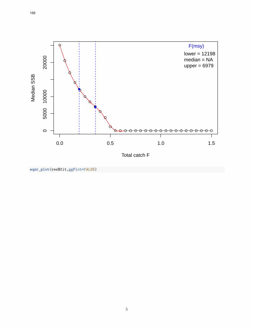
0.0 0.5 1.0 1.5
050
0010
000
2000
0
Total catch F
Med
ian
SS
B
F(msy)
lower = 12198median = NAupper = 6979
eqsr_plot(res$fit,ggPlot=FALSE)
5
159

0 2000 4000 6000 8000 10000 12000 14000
050
0000
1000
000
Predictive distribution of recruitmentfor IRISH SEA haddock,2014 WG,1−5,ANON,COMBSEX,PLUSGROUP
SSB ('000 t)
Rec
ruits
Segreg 1
#eqsim_plot2(res$sim, ymax.multiplier = 1.1, catch = FALSE) # note I modify the eqsim_plot function
Another run with with Btrigger as BPasetup <- list(data = stock,bio.years = c(2003,2012),bio.const = FALSE,sel.years = c(2003,2012),sel.const = FALSE,Fscan = seq(0,1.5,by=0.05),Fcv = Fcv, Fphi = 0.423,Blim = Blim,Btrigger = Bpa(Blim, SSBcv),Bpa = Bpa(Blim, SSBcv),extreme.trim=c(0.05,0.95))
res <- within(setup,{fit <- eqsr_fit(data, nsamp = 1000, models = "Segreg")sim <- eqsim_run(fit, bio.years = bio.years, bio.const = bio.const,sel.years = sel.years, sel.const = sel.const, Fscan = Fscan,Fcv = Fcv, Fphi = Fphi, Blim = Blim, Bpa = Bpa,extreme.trim = extreme.trim, verbose = FALSE)})
6
160

knitr::kable(t(res$sim$Refs2), digits=c(2,2,0,0,0,0))
catF lanF catch landings catB lanBF05 0.37 NA 1985 NA 6580 NAF10 0.40 NA 1916 NA 5708 NAF50 0.49 NA 924 NA 2163 NAmedianMSY NA 0.27 NA 1239 NA 9299meanMSY 0.35 0.25 2022 1233 7041 10001Medlower NA 0.19 NA 1172 NA 12188Meanlower NA 0.19 NA 1256 NA NAMedupper NA 0.35 NA 1172 NA 7048Meanupper NA 0.35 NA 1256 NA NA
eqsim_plot_range(res$sim, type="median")
0.0 0.5 1.0 1.5
020
040
060
080
010
00
Total catch F
Med
ian
land
ings
F(msy)
lower = 0.192median = 0.272upper = 0.35
F(5%)
lower = 0.155estimate = 0.366upper = 0.389
eqsim_plot_range(res$sim, type="ssb")
7
161

0.0 0.5 1.0 1.5
050
0010
000
2000
0
Total catch F
Med
ian
SS
B
F(msy)
lower = 12188median = NAupper = 7048
#eqsim_plot2(res$sim, ymax.multiplier = 1.1, catch = FALSE) # note I modify the eqsim_plot function
Another run with with no Btrigger and no errorsetup <- list(data = stock,bio.years = c(2003,2012),bio.const = FALSE,sel.years = c(2003,2012),sel.const = FALSE,Fscan = seq(0,1.5,by=0.05),Fcv = Fcv, Fphi = 0.423,Blim = Blim,Btrigger = Bpa(Blim, SSBcv),Bpa = Bpa(Blim, SSBcv),extreme.trim=c(0.05,0.95))
res <- within(setup,{fit <- eqsr_fit(data, nsamp = 1000, models = "Segreg")sim <- eqsim_run(fit, bio.years = bio.years, bio.const = bio.const,sel.years = sel.years, sel.const = sel.const, Fscan = Fscan, Blim = Blim, Bpa = Bpa,extreme.trim = extreme.trim, verbose = FALSE)})
knitr::kable(t(res$sim$Refs2), digits=c(2,2,0,0,0,0))
8
162
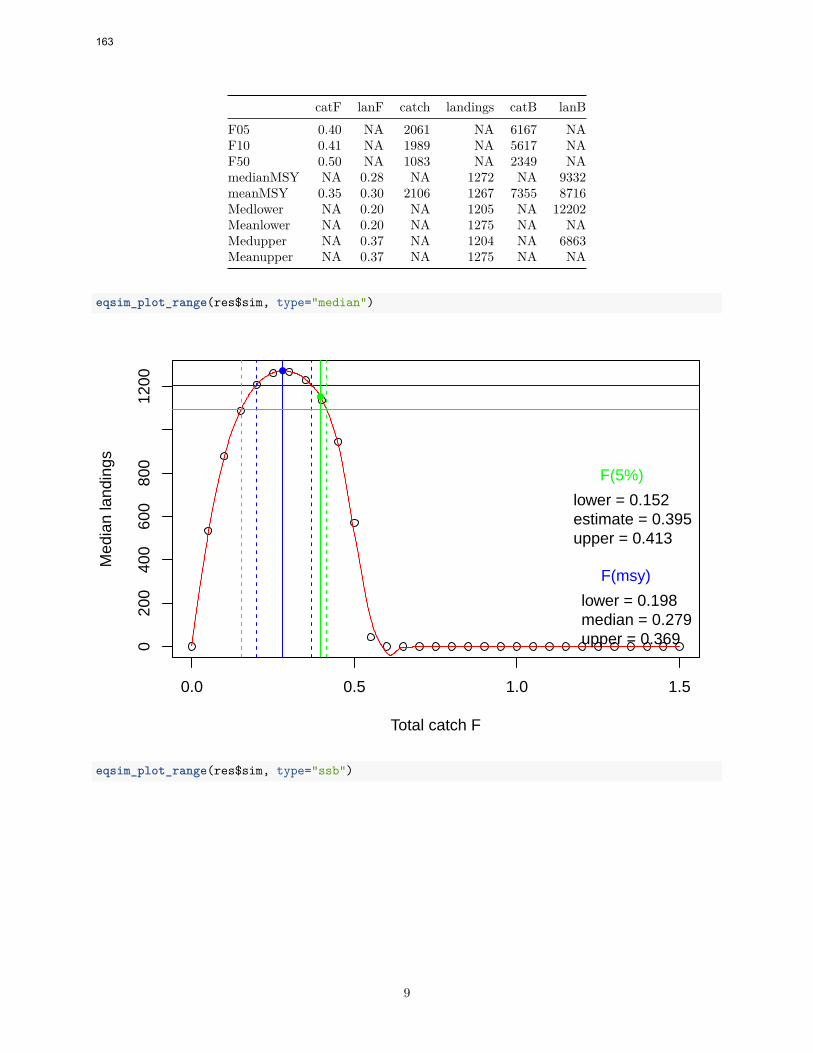
catF lanF catch landings catB lanBF05 0.40 NA 2061 NA 6167 NAF10 0.41 NA 1989 NA 5617 NAF50 0.50 NA 1083 NA 2349 NAmedianMSY NA 0.28 NA 1272 NA 9332meanMSY 0.35 0.30 2106 1267 7355 8716Medlower NA 0.20 NA 1205 NA 12202Meanlower NA 0.20 NA 1275 NA NAMedupper NA 0.37 NA 1204 NA 6863Meanupper NA 0.37 NA 1275 NA NA
eqsim_plot_range(res$sim, type="median")
0.0 0.5 1.0 1.5
020
040
060
080
012
00
Total catch F
Med
ian
land
ings
F(msy)
lower = 0.198median = 0.279upper = 0.369
F(5%)
lower = 0.152estimate = 0.395upper = 0.413
eqsim_plot_range(res$sim, type="ssb")
9
163
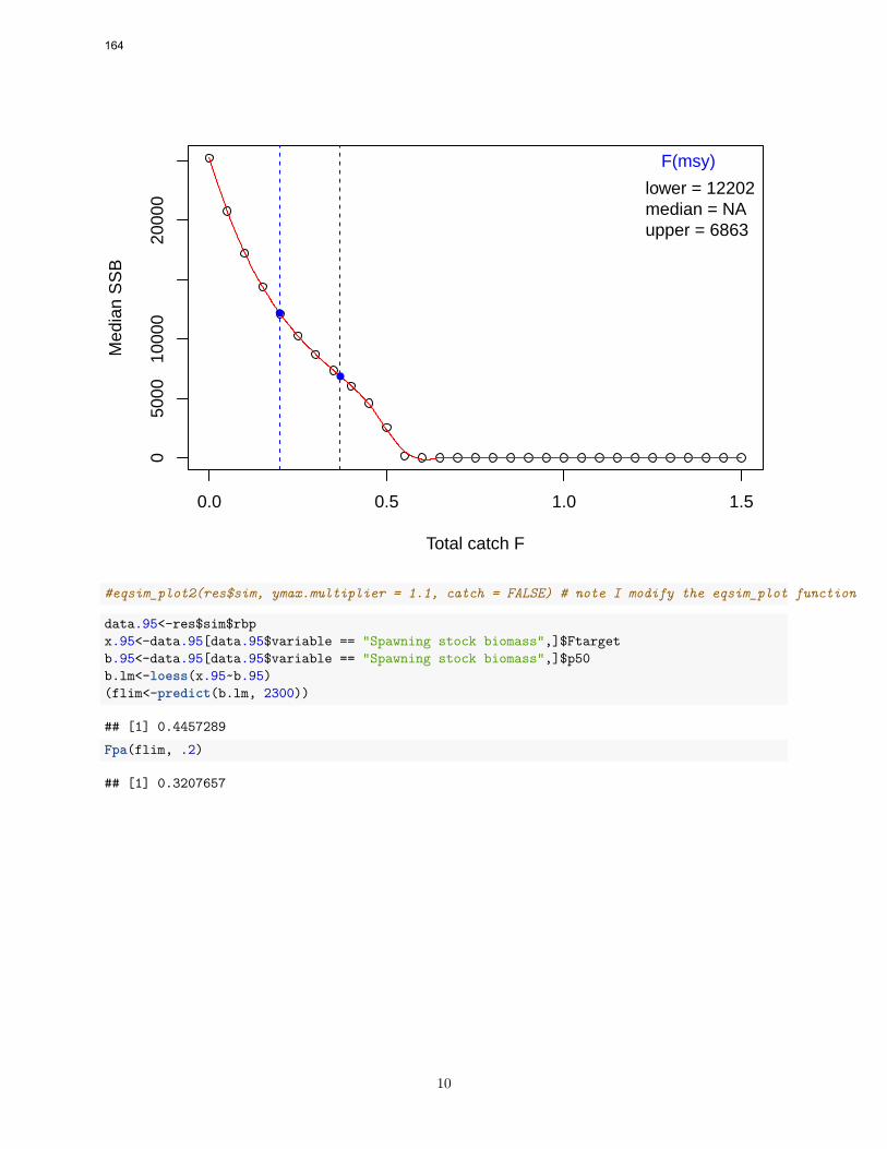
0.0 0.5 1.0 1.5
050
0010
000
2000
0
Total catch F
Med
ian
SS
B
F(msy)
lower = 12202median = NAupper = 6863
#eqsim_plot2(res$sim, ymax.multiplier = 1.1, catch = FALSE) # note I modify the eqsim_plot function
data.95<-res$sim$rbpx.95<-data.95[data.95$variable == "Spawning stock biomass",]$Ftargetb.95<-data.95[data.95$variable == "Spawning stock biomass",]$p50b.lm<-loess(x.95~b.95)(flim<-predict(b.lm, 2300))
## [1] 0.4457289
Fpa(flim, .2)
## [1] 0.3207657
10
164

ICES WKIrish3 REPORT 2017 | 165
Annex 10: Stock Annexes
The table below provides an overview of the stock annexes updated at WKIrish3. Stock Annexes for other stocks are available on the ICES website Library under the Publication Type “Stock Annexes”. Use the search facility to find a particular Stock Annex, refining your search in the left-hand column to include the year, ecoregion, spe-cies, and acronym of the relevant ICES expert group.
STOCK ID STOCK NAME LAST UPDATED LINK
cod.27.7a Cod (Gadus morhua) in Division 7.a (Irish Sea)
March 2017 cod.27.7a
had.27.7a Haddock (Melanogrammus aeglefinus) in Division 7.a (Irish Sea)
March 2017 had.27.7a
whg.27.7a Whiting (Merlangius marlangus) in Division 7.a (Irish Sea)
May 2017 whg.27.7a
ple.27.7a Plaice (Pleuronectes platessa) in Division 7.a (Irish Sea)
May 2017 ple.27.7a

166 | ICES WKIrish3 REPORT 2017
Annex 11: Summary report from external panel
Daniel Howell, Jim Ianelli and Rebecca Lauerburg acted as external experts for the WKIrish3 benchmark of the Irish Sea Whiting, Cod, Haddock, Plaice and Herring stocks. The panel reviewed modelling approaches used for assessment concerning suitability for advice at the workshop held at the Marine Institute in Oranmore, Ire-land 29 January–4 February 2017.
The reviewers highlight the efforts of all working group participants during the benchmark process. All requests from the panel were addressed extensively from the researchers during the workshop which enhanced the panel’s understanding of the individual stock assessments. In summary, the work conducted by the working group during the benchmark process greatly improved the consistency in assessment applications and was successful in implementing valuable information in the man-agement process.
In the following section the panel outlines the central topics of each stock assessment that were addressed during the workshop along with conclusions on the eligibility of the current assessment for providing advice and additional recommendations for fu-ture work.
Recommendations for future work
Discard estimation approaches
Specifically for plaice the issue arose in which the method which used the recent pe-riod for which data were available to expand and estimate historical discards was problematic because of known changes in the fisheries. Historically more plaice were landed and in recent years, a much larger fraction is estimated to be discarded.
Disaggregating fishery data
For the cod and haddock assessments (and perhaps whiting?) the models would be improved by splitting the fisheries such that the Nephrops and bycatch fisheries were treated separately from the directed fishery. This would be preferred for a number of reasons. Namely, the advice could be tailored to account for the expected effort in the bycatch fishery (and concomitant impacts) relative to future potential allowances in directed fisheries.
Natural mortality specifications / estimation
The group noted that in general the following treatment / specification of natural mortality advanced for these stocks was considered extensively (see section of main report titled “Derivation of natural mortality (M) values for cod, haddock, whiting, plaice and herring”). This should be considered further, specifically as relates to the potential for evaluating time-varying values (similar to what’s being done in the North Sea from multispecies model estimates).
Consideration of environmental factors
In general, fish distributions in the Irish Sea seem likely to be affected by environ-mental drivers and this seems to be a benefit of having a regional benchmark. How-ever, common environmental effects on how fish distributions may change due to interannual variability and longer term factors could have been provided and dis-

ICES WKIrish3 REPORT 2017 | 167
cussed at least in general terms. Application of the ICES FISHDISH working group document might have been helpful in setting the stage for potential trends/changes in distributional characteristics of stocks within this region.
Cod
Issues addressed at the benchmark
The current assessment is based on survey trends and the analysts provided results from SAM (a work in progress), and ASAP were presented. The group agreed that the analyst’s choice of proceeding with the ASAP modelling framework was appro-priate. Alternative model configurations (some 20 or so) were evaluated and a candi-date configuration was selected based on evaluations of residuals, the likelihood values of data fitting and model assumptions, and interpretation of known fishery patterns (e.g., uncertain catch totals and shifts to being primarily a bycatch fishery).
Use of final stock annex as basis for providing stock advice
The review panel felt able accept the final model as suitable for use in assessments, and felt that a reasonable job had been done in exploring and evaluating the model settings. The group noted that the model selected had fishery selectivity in the most recent period that declined significantly in the oldest ages and that should the stock increase and a fishery redevelop, that a change in selectivity where older ages are more fully selected might be considered.
Haddock
Issues addressed at the benchmark
The group evaluated a large number of model configurations (within the ASAP mod-el framework) The final model included FSP survey, 3 selectivity blocks, a considera-tion of uncertainty in catches during the period 2004–2007, and downweighting the influence of the internal penalty on the stock–recruitment relationship.
Use of final stock annex as basis for providing stock advice
The review panel felt able accept the final model as suitable for use in assessments, and felt that a reasonable job had been done in exploring and evaluating the model settings. They noted that, as with cod, future changes in fishery selectivity are likely should the directed fishery redevelop and that this should be a consideration in up-dating advice to ICES.
Herring
Issues addressed at the benchmark
The key issue for herring addressed at the benchmark was that the model results have been considerably lower than that suggested by the acoustic surveys. A new SSB acoustic series was therefore presented, with the aim of using this as an absolute estimate (i.e. q=1) in the model tuning. An evaluation of the impact of introducing this new acoustic SSB tuning series, both with and without fixed catchability (q=1), was conducted using the SAM modelling framework. When the catchability was not fixed the model estimated a very high catchability (q=3.8), indicating almost a four-fold difference between the survey and model biomass estimates.

168 | ICES WKIrish3 REPORT 2017
The analysis was complicated by a number of factors. Within the SAM model, the ability to ascertain what aspects of the model process errors and/or data components are tending to underestimate the spawning biomass estimated using acoustic meth-ods was problematic. Furthermore the version of SAM used was not well suited to exploring sensitivity issues around survey q or CV, with hardcoded changes required at each stage. Partly as a result of these difficulties, analysing the effect of the differ-ent proposed model variants was difficult.
There was extensive, and somewhat inconclusive, discussion around the quality of the survey, it’s suitability as an absolute estimate, and the degree to which the survey had been evaluated by other working groups. The methodology used is consistent with other approaches to develop acoustic-trawl survey biomass estimates, and the survey appeared to present a reasonable, if somewhat noisy, SSB estimate. The issue of discussion centred only on the issue of whether to use the survey as a relative or absolute estimate.
Use of final stock annex as basis for providing stock advice
The new SSB tuning series only covers the latter part of the time-series of the model (2007 onwards). With q set to one for this survey, the model gives a strong increase in modelled SSB around the year the acoustic SSB survey begins. This implies that the model is forcing an increase to occur at the start of the survey series, which is likely resulting in an artificially high stock post 2007 relative to the earlier period (which has no fixed q survey data). The result of only having a forced catchability for part of the time-series is thus to produce an over rapid rise in the stock and distort the histor-ical stock dynamics. The review panel therefore does not believe that this forms an acceptable basis for an assessment.
Some reviewers are not, in principle against fixing q=1 for an acoustic survey for this stock. One reviewer (JI) was comfortable treating the survey as an absolute index of biomass provided an appropriate CV was used. One reviewer (RL) did not agree to use the new acoustics survey in terms of absolute estimates without justification of the underlying model assumptions that are used to calculate the SSB from the hydro-acoustics data and thoroughly presentation of uncertainties and error estimates. However, all reviewers agreed that diagnostics to evaluate models with this option were insufficient and hence the panel was unwilling to accept as the basis for an as-sessment.
Subsequent to the review, a number of email exchanges on this topic occurred along with updated diagnostics and some further evaluation. Our discussions were provid-ed to the HAWG for further consideration.
Recommendations for further work
The review panel strongly recommends further work on this topic to try to resolve the discrepancy between the survey and model levels of biomass, and supports the WG recommendation for the forthcoming HAWG assessment group to decide on ToRs for an inter-benchmark focussed specifically on this issue. We consider that it would be preferable for future work on this stock to include a reviewer with greater knowledge of the stock.
As part of the analysis we recommend that, if the q was to be fixed in future assess-ment model, then a sensitivity of the resulting population estimate to the choice of q should be conducted. A situation where SSB (and hence catch) is sensitive to a (somewhat uncertain) choice of survey CV would be rather unfortunate. It would

ICES WKIrish3 REPORT 2017 | 169
also seem likely from the analysis at this WG that any absolute estimates would need to apply to the whole model time-series to avoid distorting stock dynamics.
The review panel notes that the standard ICES benchmark workflow (issues list, data evaluation meeting prior to the benchmark) has not been well followed for the her-ring (although it was for the other stocks). This contributed to the situation where magnitude of the proposed change, and major problems in the proposed assessment model, were not identified until late in the physical meeting. We would recommend that future work on this stock be more structured to avoid a repetition of this issue.
Plaice
Issues addressed at the benchmark
A variety of methods (AP, XSA, SAM, and SPICT) were presented with the most ex-tensive being the application of the SAM modelling framework for the assessment. Sensitivities ranged over natural mortality, discard approaches, retrospectives, time-series lengths, data omissions (sensitivities to inputs), linkages to plus group, and a number of other aspects related to random walk specifications. The biggest effect was discard approach selected followed by M specifications. The updated runs made dur-ing the week with the Lorenzen “shape” but scaled to have the mean M (for the older ages) were most defensible because the original M estimate was based on an earlier tagging study.
The Panel considered these sensitivities as useful and going forward, thought that the SAM model configuration with the higher discard estimates, using 9+ instead of 8+, correlation flag set to 2 for F-over ages, Lorenzen M vector scaled to 0.12 for older ages, updated SSB index (to be consistent with maturity at age / size assumption).
Use of final stock annex as basis for providing stock advice
Discard estimation was evaluated against size-selection expansions by ages and the updated results of this during the week caused unacceptable patterns in the retro-spective analyses (lack of convergence, etc.), and in some cases complete lack of con-vergence. The working group will revisit the discard estimation and at such time the SAM assessment model framework will be reviewed by the externals and potentially accepted for the annex and upcoming advice.
As a follow-up a well-documented revision of the discard estimation method was presented to the reviewers. Three different approaches to provide discard reconstruc-tions were evaluated. The low and high discards scenarios were rejected since both were more inaccurate compared to the third scenario. The medium discards scenario was chosen for input to the assessment used for management since it was the most data-driven approach and was consistent with the key conclusions drawn from the historical data. Discard estimates for the period 1980–2015 were used for the baseline stock assessment run, since there is no information on the minimum landing size pri-or to 1981. The panel felt comfortable with the final discard estimates that were used in the assessment model.
Apart from the discard issue, the review panel was happy to accept the proposed model configuration and appreciated the detailed examinations that were carried out prior to and during the benchmark review.

170 | ICES WKIrish3 REPORT 2017
The group reviewed the selection choices for near-term projections for this stock and agreed with the analysts view that a 3-year mean for partial Fs and landing fractions was appropriate, as was the median recruitment estimates from 1992–2015.
Whiting
Issues addressed at the benchmark
A characteristic of the available data was that the recent period (2004–2015) suggest greater negative slopes for the older whiting in both the surveys and in the fishery data. The fishery data was partially explainable because the catch has shifted to pri-marily bycatch in the Nephrops fishery but the survey data suggest a higher mortality even though the catch has remained relatively low over this period. This was dis-cussed at length and may reflect a change in natural mortality.
The current assessment is based on survey trends and the analysts provided results from XSA and ASAP were presented. The group agreed that proceeding with the ASAP model framework for this assessment was appropriate. A broad array of con-figurations were evaluated and the group stepped through decision points for final specifications. This included evaluating sensitivities for time-varying natural mortali-ty (based on estimated changes in mean weight-at-age via the Lorenzen formula), the number of periods selectivity was allowed to change, specified CV on catch biomass estimates, effective sample sizes for composition data, CV assumed for index data, including FSP survey explicitly, and some minor output changes such as age range over which F was averaged.
Use of final stock annex as basis for providing stock advice
The review panel felt able accept the final model as suitable for use in assessments, and felt that a reasonable job had been done in exploring and evaluating the model settings.
Regional Benchmark General comments
In general having a Regional Benchmark covering similar fish was helpful in that it identified common trends, and allowed consistency in approaches between stocks. The fact that the same model was chosen for many of the stocks evaluated here facili-tated this partial harmonization of approaches between stocks. It also allowed for the different stock assessors to borrow strength from each other, which facilitated the work. This is a region where many of the stocks experienced strong declines in bio-mass, and consequent changes in selectivity, at around the same time.
Having herring in the list of stocks was problematic due to the lack of herring exter-nal experts and the fact that a long running intractable problem was included in the benchmark at a rather late stage (the proposed survey had not been evaluated at the data workshop). It may be sensible if regional benchmarks become the norm to have a separate place to address particularly difficult issues (where these can be identified in advance), and avoid them dominating over much of the regional benchmark.
The panel was presented with a wide range of model approaches to assess the differ-ent Irish Sea fish stocks subject to WKIrish3. A lot of work has been carried out on model choice and model improvement by sensitivity analyses of model settings. The model settings for the Irish Sea herring stock could not be agreed on during the meet-

ICES WKIrish3 REPORT 2017 | 171
ing and the panel suggested a revision of the model settings during an inter-benchmark workshop.
The panel felt able to accept the final model settings for whiting, haddock and cod stocks and considered those model to be useful to provide the basis for stock assess-ment and advice. After a successful resolution to the plaice discard estimation issue, the same can be said for the plaice assessment. A reasonable job had been done in exploring and evaluating the model settings.