icewin - trimis.ec.europa.eu · passenger transportation by car is consumed by the households and...
TRANSCRIPT

SEVENTH FRAMEWORK PROGRAMME THEME 7 Transport
IceWin Innovative Icebreaking Concepts for Winter Navigation
Grant no 234104
D3.1 Oil Reserves and Contracts
Work Package: WP3
Deliverable type: Report
Contractual date of delivery: 28.02.2010
Actual date of delivery: 28.02.2010
Authors: Delhaye Eef (TML) Heyndrickx Christophe (TML) Vanpeteghem Veerle (TML)

List of Beneficiaries
Beneficiary Number *
Beneficiary name
Beneficiary short name
Country Date enter
project Date exit project
1 (coordinator)
Valtion Teknillinen Tutkimuskeskus
VTT FI 1 24
2 Hama Investeeringud
HI EST 1 24
3 TML TML BEL 1 24
4 Aker Arctic Technology
AARC FI 1 24

IceWin Grant no: 234104
Executive Summary
The IceWin project aims to find out what benefits can be attained by adopting innovative concepts and operations of icebreakers and/or by utilizing a new kind of agreement system in the Baltic Sea.
The ice cover of the Baltic Sea Motorway varies considerably from year to year. Hard ice conditions markedly influence traffic conditions. Even at current transport levels, the current icebreaker fleet available in the Baltic Sea is incapable of providing a satisfactory level of service in a hard ice winter. At the same time export, especially oil transports from Russia to other parts of Europe, is growing.
The goal of this task report is to determine the importance of transport on the Baltic Sea. This is the first step within Work Package 3, in which the effect of a hard ice winter with insufficient icebreaking resources on the European economy is analysed. Given the geographical location the focus lies on transport flows between ten countries located around the Baltic Sea. In particular, special attention will be given to the maritime trade flows between EU member states Sweden, Finland, Estonia, Latvia, Lithuania, Poland, Denmark, Germany and non-EU member states Norway and Russia.
The analysis focussing on the elements determining the importance of an oil supply interruption, showed that the possible effect is likely to be small, or even negligible. The main reasons for this result are that
- most likely oil transport would be given priority when icebreaking resources are insufficient
- on average, only 10% of total oil consumption in the EU could be hindered
- alternative oil supply sources are feasible for most EU countries
- the use of the 90 day oil reserve is a valid option for such a local, seasonal disruptions
Hence, we extended our analysis to the transport of all goods, focussing on the imports for countries around the Baltic Sea. This analysis showed that also the import of non-oil goods would be affected. This problem is potentially larger than the import of oil as
- these goods are less likely to get priority assistance
- the availability of large reserves – up to 90 days in the case of oil products – is less likely
3 of 54 pages


IceWin Grant no: 234104
Contents
Executive Summary .............................................................................................................3
Terminology ..........................................................................................................................7
1 Introduction .................................................................................................................11
1.1 Objective of IceWin.............................................................................................11 1.2 Objective of WP3 – Consequences of Insufficient Resources ............................11 1.3 Objective of task 3.1 ............................................................................................12
2 Background..................................................................................................................14
3 Importance of Oil in the European Economy...........................................................16
3.1 Use of oil within different sectors........................................................................17 3.2 Origin of the Oil used within the EU...................................................................18 3.3 Importance of oil transport over the Baltic Sea ...................................................21
3.3.1 Pipelines ..................................................................................................23 3.3.2 Oil tankers ...............................................................................................24
3.4 Reserves & Contracts...........................................................................................24 3.4.1 Reserves ..................................................................................................25 3.4.2 Contracts..................................................................................................26 3.4.2.1 Contracts with Russia..............................................................................26 3.4.2.2 Between EU countries.............................................................................26
4 Analysis of transport flows over the Baltic Sea ........................................................27
4.1 Transport of goods over the Baltic Sea................................................................27 4.1.1 Import into Estonia..................................................................................29 4.1.2 Import into Finland..................................................................................30 4.1.3 Import into Lithuania ..............................................................................30 4.1.4 Import into Latvia....................................................................................31 4.1.5 Import into Poland...................................................................................32 4.1.6 Import into Sweden .................................................................................33
4.2 Of oil goods .........................................................................................................33
5 What could be the effect of interruptions in transport over the Baltic Sea...........35
5.1 Interruptions in oil supply....................................................................................35 5.2 Interruptions in import of other goods.................................................................35 5.3 Link with EDIP....................................................................................................36
5.3.1 A price increase.......................................................................................36 5.3.2 Actual stop of supply...............................................................................37
5 of 54 pages

IceWin Grant no: 234104
References ...........................................................................................................................38
1 Annex 1: Description of the EDIP model. .................................................................39
1.1 Introduction..........................................................................................................39 1.1.1 State-of-the-art ........................................................................................40 1.1.2 Model overview ......................................................................................40 1.1.3 Applicability............................................................................................42
1.2 The EDIP Model structure ...................................................................................42 1.2.1 Production ...............................................................................................43 1.2.2 Consumption ...........................................................................................45 1.2.3 Transport sector.......................................................................................47 1.2.4 International trade ...................................................................................48 1.2.5 Labour market .........................................................................................50 1.2.6 General equilibrium structure..................................................................51 1.2.7 Government and its policy instruments...................................................52 1.2.8 Emissions ................................................................................................53 1.2.9 Recursive dynamics.................................................................................53
6 of 54 pages

IceWin Grant no: 234104
Terminology
Baltic Sea Motorway
Sea routes to the ports of Sweden, Finland, Russia, Estonia, Latvia, Lithuania, Poland, Germany and Denmark in the Baltic Sea.
.
Bbl/day Barrels per day
ice winter Ice conditions in traffic on water (scope and thickness of ice, pressure ridges, etc.) in winter, e.g. ice winter 2007-08.
level of service Quality of icebreaker service, mainly waiting time and pass-through time of a merchant vessel.
7 of 54 pages

IceWin Grant no: 234104
List of Figures Figure 1. Motorway of the Baltic Sea (Source: Ministry of Transport and Communications
of Finland ..................................................................................................................... 15 Figure 2. Hard, mild and average ice winters in the Baltic Sea. .......................................... 15 Figure 3: Gross Inland Consumption – EU27 by fuel.......................................................... 16 Figure 4: Consumption of oil in the EU............................................................................... 18 Figure 5: Origin of oil consumed within the EU in 2005..................................................... 19 Figure 6: Russians export in BBL/day – mode of transport................................................. 22 Figure 8: Transport over the Baltic Sea according to NSTR class....................................... 28 Figure 9: Origin of transport over the Baltic Sea ................................................................. 28 Figure 10: Import via the Baltic Sea into Estonia according to NSTR classes .................... 29 Figure 11: Import via the Baltic Sea into Finland according to NSTR classes.................... 30 Figure 12: Import via the Baltic Sea into Lithuania according to NSTR classes................. 31 Figure 13: Import via the Baltic Sea into Estonia according to NSTR classes .................... 32 Figure 14: Import via the Baltic Sea into Poland according to NSTR classes..................... 32 Figure 15: Import via the Baltic Sea into Sweden according to NSTR classes ................... 33 Figure 16: Origin of mineral fuels (NSTR 2), crude oil (NSTR 3) and petroleum products
(NSTR 10) on the Baltic Sea........................................................................................ 34 Figure 17: Destination of mineral fuels (NSTR 2), crude oil (NSTR 3) and petroleum
products (NSTR 10) on the Baltic Sea ......................................................................... 34
8 of 54 pages
IceWin Grant no: 234104
List of Tables Table 1: Share of oil import to the EU27 from Russia......................................................... 21 Table 2: NSTR codes ........................................................................................................... 27 Table 3: Share of import into Estonia via the Baltic Sea ..................................................... 29 Table 4: Share of import into Finland via the Baltic Sea ..................................................... 30 Table 5: Share of import into Lithuania via the Baltic Sea .................................................. 30 Table 6: Share of import into Latvia via the Baltic Sea ....................................................... 31 Table 7: Share of import into Poland via the Baltic Sea ...................................................... 32 Table 8: Share of import into Sweden via the Baltic Sea..................................................... 33
9 of 54 pages


IceWin Grant no: 234104
1 Introduction
Within this chapter we first discuss the general objective of the IceWin project; next, we turn to the focus of Work Package 3 – Consequences of insufficient resources. Finally, we review the goal of this task report – Oil Reserves and Contracts.
1.1 Objective of IceWin
The ice cover of the Baltic Sea Motorway varies considerably from year to year. The northern parts freeze every winter. In a hard ice winter it freezes completely. Despite the climate change, hard ice winters occasionally occur in the Baltic Sea.
Even the current icebreaker fleet available in the Baltic Sea is incapable of providing a satisfactory level of service in a hard ice winter. The combination of growing traffic volumes and the hard ice winter will mean serious difficulties for industrial and commercial transports.
Some of the current icebreaker fleet will reach the end of its lifespan in the 2010s. It is evident that replacement investments will not yield a satisfactory level of service in hard ice winter conditions. Considering the growing traffic volumes, a satisfactory level cannot be reached even in an average ice winter. A large oil tanker, for instance, requires simultaneous assistance from two traditional icebreakers that together are capable of breaking a sufficiently wide channel through the ice.
The objective of the IceWin project is to find out what benefits can be attained in the level of service of icebreaking assistance, in logistics and especially in oil transports, and with regard to environmental emissions and risks, by
a) adopting the new technical solutions, and/or
b) utilising the new type of agreement system
The new technical solutions may be the innovations that are alone capable of breaking a sufficient wide channel also for overwide merchant vessels, e.g. oil tankers. The technical solutions have already completed but not introduced.
The new agreement system to be developed would be based on the utilization of icebreaking capability of independently ice-going merchant vessels. It is important that jointly accepted rules could be enforced for cases where the capacity of conventional icebreakers is not sufficient.
1.2 Objective of WP3 – Consequences of Insufficient Resources
In the third work package the effect of the hard ice winter in a case where icebreaking resources are insufficient will be researched. The main objective is to develop a
11 of 54 pages

IceWin Grant no: 234104
methodology for the calculation of effects upon European economy, production, costs and competitiveness in case transport flows via the Baltic Sea would be interrupted for some time. The general methodology developed within this workpackage will be based on the existing general equilibrium model EDIP. EDIP itself is the European economic-energy-environment-equity model developed by TML during the REFIT project (FP6-022578). The EDIP model has a single structure for all EU countries. It is a single model with 31 different versions, which are estimated using a country-specific social accounting matrices for the EU27 + CH + NO + TR + HR.
EDIP is focused on the transportation sector. Households and domestic sectors use transport services in their consumption and production activities. The transport services represented in the EDIP model are differentiated by two distance-based classes (below 500km and above 500km) and by all main types of transport modes (land (road and rail), water and air). Passenger transportation by car is consumed by the households and firms themselves using fuel and car vehicles.
EDIP also has quite detailed energy component: households and firms can choose between consuming different types of energy including electricity, coal, gas and refined oil with a different contribution to emission levels.
A more elaborated description of the EDIP model can be found in annex 1.
Initially, the idea was to focus on interruptions and breakdowns on oil transports departing from Russian ports to other European ports. However, further analysis showed that in hard winter conditions and insufficient icebreaking resources oil tankers would be treated with a high assistance priority. It would be quite apparent that even in hard ice conditions there would not be long breaks or long waiting times for assistance during navigations for oil transport. Moreover, as the analysis within this task will show, European Member states are obliged to hold oil reserves for 90 days. Therefore, we decided to extend the analysis and to consider the transport flows of all the main goods transported.
1.3 Objective of task 3.1
This document is dedicated to the first of three tasks within workpackage 3. The initial goal of this task was to make a review of the existing oil reserves of the EU and the long term (in most case 25 years long) oil supply contracts between many European member states and Russia. This would allow the consortium to integrate the representation of restrictions in the short-run oil supply (both from reserves and contracts) in the EDIP model. Representation of oil supply would take into account both the fixed part of supply in the form of reserves and its variable part in terms of contracts, which might allow for some flexibility in terms of the amount of oil supplied from countries other than Russia. Given the remarks made earlier, we extended this analysis and included the other goods transported as well.
12 of 54 pages

IceWin Grant no: 234104
In summary, this task is dedicated to data collection and a first analysis of the data, which will in a next stage be fed into the EDIP model.
The structure of this deliverable is as follows. We first sketch the general background of the problem. Next we focus on the importance of oil for the European economy by discussing the consumption of oil, the different sources and the oil reserve obligation within the European Union. This will give us a first idea on the possible magnitude of the consequences of an oil supply disruption on the European Economy. The following chapter deals with transport flows of all goods over the Baltic Sea. The goal of this chapter is twofold. Firstly, we want to get an idea of the importance of transport over the Baltic Sea, secondly, the data discussed here will be used further on within WP3 as an input for the EDIP model. Hence, we conclude this deliverable with a short discussion on how this data will be used within EDIP. A description of this model can be found in annex 1.
13 of 54 pages

IceWin Grant no: 234104
2 Background
The Baltic Sea is essentially a shared shallow lake of the EU states and Russia. Since the end of the Cold War, economic activity in and around the Baltic, especially sea transport, has grown dramatically. Today 15 per cent of world sea transport takes place in these constricted waters. Statistics1 show that about 1,800 vessels are on the move in the Baltic at any given time. The fastest-growing group of vessels are oil tankers. Their numbers are stunning. More than 150 million tons of crude now annually transit the Danish Straits. Russia is currently building an additional oil pipeline and a new export terminal on the Gulf of Finland that will add another 50 million tons a year to this traffic2. The consensus estimate at the moment is that crude oil exports shipped via the Baltic will rise 40% by 2015. However, this transport could be hindered by hard winters when the sea freezes over.
The ice cover of the Baltic Sea Motorway (Figure 1) varies considerably from year to year. The northern parts of the Motorway freeze every winter. In a hard ice winter, the Motorway freezes completely. Figure 2 shows the situation in the ice winter 1986-87 when the route froze up until the straits of Denmark. Traffic conditions were difficult in the ice winter 2002-03, even though the ice winter was classified as average. In the worst case, merchant vessels bound for Russian ports but stuck in the ice had to wait for icebreaker assistance for as long as two weeks. Despite climate change, hard ice winters occasionally occur in the Baltic Sea, especially in the Gulf of Finland and the Gulf of Bothnia.
In a report3 of European Commission export forecasts has been introduced. The export will grow in Russia 2.4 fold in 2007-2030 as they do also in Baltic countries (Estonia, Latvia, and Lithuania). The growth of export has a significant effect particularly on sea transports, especially oil transports from Russia to other parts of Europe. As will become clear later on, the European economy is increasingly dependent on oil transported from Russia.
The current icebreaker fleet available in the Baltic Sea is incapable of providing a satisfactory level of service in a hard ice winter. In hard conditions and with the current traffic volumes, 11 icebreakers would be needed in the Gulf of Finland alone in order to reach a satisfactory level of service, where in fact only 6 icebreakers are currently available (Finland 3, Estonia 1 and Russia 2). The combination of growing traffic volumes and hard ice winter conditions is like a time bomb. At the critical point when it explodes, it will mean serious difficulties for industrial and commercial transports. This may critically hamper e.g. the availability of oil in view of European energy supply. The situation undoubtedly affects oil price and undermines European competitiveness. Furthermore, it also hinders the import of basic goods in countries around the Baltic Sea, affecting the general economy of those countries and their exports, affecting their competitiveness. 1 HELCOM Stakeholder Conference on the Baltic Sea Action Plan (2006), Maritime transport in the Baltic Sea. Draft HELCOM Thematic Assessment, 7 March 2006 2 Borisocheva, K. (2007), Analysis of the Oil-and Gas-Pipeline-Links between EU and Russia – An account of intristic interests, CERE 3 The Northern Transit Axis, Final Report, November 2007, European Commission, Directorate-General Energy and Transports
14 of 54 pages

IceWin Grant no: 234104
EST
DEN
FIN SWE
POL GER
LAT
LIT
RUS
Figure 1. Motorway of the Baltic Sea (Source: Ministry of Transport and Communications of
Finland
hard ice winter, year 1986-87
ice cover 337 000 km²
mild ice winter, year 1991-92
ice cover 122 000 km²
average ice winter, year 1994-95
ice cover 206 000 km²
Figure 2. Hard, mild and average ice winters in the Baltic Sea.
In the next chapter we discuss the importance of oil in the European economy.
15 of 54 pages

IceWin Grant no: 234104
3 Importance of Oil in the European Economy
The European Union has large coal, oil, and natural gas reserves. There are six oil producers in the European Union, primarily in North Sea oilfields. The United Kingdom by far is the largest producer, however Denmark, Germany, Italy, Romania and the Netherlands all produce oil. Europe produces, as a whole about 5,195,218 barrels a day (2008)4, making it –as a whole - the 7th largest producer of oil in the world. This number includes the production of oil by Norway – about 2,465,955 barrels a day (2008). However, it is also the world's 2nd largest consumer of oil, consuming much more than it can produce, at 16,128,131 (2008) barrels a day5. Hence Europe currently imports 82% of its oil, making it the world’s leading importer of these fuels. Much of the difference comes from Russia and the Caspian Sea basin.
When we consider the importance of oil in the energy mix, Figure 3 shows that oil accounts for about 37% of all consumption of energy, making it the most important energy source. Figure 3 also shows that its share has not decreased over the years.
Source: Eurostat, December 2008 * Electrical Energy and Industrial Waste
Gross Inland Consumption - EU27by fuel (in Mtoe)
Solid fuels
Oil
Gas
Nuclear
Renewables
0
250
500
750
1000
1250
1500
1750
1990
1991
1992
1993
1994
1995
1996
1997
1998
1999
2000
2001
2002
2003
2004
2005
2006
Mtoe
0
250
500
750
1000
1250
1500
1750
Year 2006
Oil36.9%
Gas24.0%
Nuclear14.0%
Renewables
7.1%
Other *0.2%
Solid fuels
17.8%
Other *
Figure 3: Gross Inland Consumption – EU27 by fuel
Source: Energy Pocket Book (2009)
There are of course important differences between countries6. For example, oil is the only energy source (100%) in Malta. Also in Ireland (55%), Greece (58%), Cyprus (97%) and Luxembourgh (63%), more than half of all energy consumed is oil. Countries with a relatively low share – smaller than 25% - of oil are Bulgaria, Czech Republic, Estonia, Poland and Slovakia. Note that the share of oil might increase in the short term for some countries who opted for a nuclear phase out. For example Belgium opted for a nuclear phase out, while in 2006, 20% of its energy consumption had a nuclear source. The 4 US Energy Information Administration, International Energy Statistics, Total Oil Supply, http://tonto.eia.doe.gov/cfapps/ipdbproject/IEDIndex3.cfm?tid=5&pid=53&aid=1 5 US Energy Information Administration, International Energy Statistics, Total Consumption of Petroleum Products, http://tonto.eia.doe.gov/cfapps/ipdbproject/IEDIndex3.cfm?tid=5&pid=54&aid=2 6 Energy Pocket Book (2009)
16 of 54 pages
IceWin Grant no: 234104
question is by which type of energy this will be replaced. At the moment, the countries with the highest share of renewable energy are Latvia (with 31%) and Sweden (with 29%).
In the next paragraphs we discuss the use of oil within the different economic sectors, the origin of the oil consumed within the EU and the relative importance of oil travelling via the Baltic Sea. In the next paragraph, we focus on the oil reserves and the contracts within and with the European Union. Finally, we give a first qualitatively assessment of the possible effects of an interruption and make a first link with the further analysis which will use the EDIP model.
3.1 Use of oil within different sectors
Oil supply disruption is likely to have serious negative impacts on the economy, depending on the relative size and the duration of the disruption. Some sectors are particularly dependent on the regular supply of oil and/or petroleum products. In order to determine the impact of disruptions in oil supply it is necessary to know the oil intensity of all sectors. In general, as can be seen from the figure below, transport is by far the biggest user of oil in the EU (31%) and oil accounts for 97% of energy consumption in this sector. Households spend 13.6% of their total final consumption on transport, mostly by road and air. Part of this transport is not really needed (holidays, leasure), but an important part is the base for social organization and adequate labour force mobility. Therefore, via transport, oil disruption could also have a secondary effect on other sectors. Oil is also consumed by households in the form of heating. Furthermore it plays an important role in the industry. In the chemical industry, oil is the main feedstock and energy source at the same time. In fisheries sector, fuel costs constitute more than 30% of the value of EU fish landings. Oil only plays a limited role in the electricity sector (5%). However, for some south European countries, power supply depends for some 13-19% on oil fired power plants, while in Cyprus and Malta this rises to about 100%.
17 of 54 pages

IceWin Grant no: 234104
Consumption of oil in the EU
47%
8%14%
8%
9%
9% 5%transportaviationnon-energy usesotherindustryhouselholdselectric power
Figure 4: Consumption of oil in the EU
Source: European Commission (2008), Commission Staff Working Document, accompanying document to the Proposal for a Directive of the Council Imposing an obligation on Member States to maintain minimum stocks of crude oil and/or petroleum products – Impact Assessment.
3.2 Origin of the Oil used within the EU
In 2006, 85% of the oil consumed within the European Union came from outside the European Union. Most (19 countries) import more than 95% of their oil consumption. Only Denmark has a net export, while Romania has an import dependency of 44% and Great Britain of only 9%7. Few European countries produce oil – with Norway producing 47%, Great Britain 30% and Denmark 6% of the total European production.
As can be seen from Figure 5, the Russian Federation is the EU's most important single supplier of oil, accounting for over 30% of the EU consumption of oil and gas. The main importers from Russia are Great Britain, France, Germany and Spain.
7 Energy Pocketbook (2009)
18 of 54 pages

IceWin Grant no: 234104
Oil import to the EU (25)
30%
17%11%
9%
6%
5%
4%3%
2%2% 2%
9%
Russia
Norway
Saudi Arabia
Libya
Iran
Kazakhstan
Algeria
Nigeria
Iraq
Mexico
Syria
Other
Figure 5: Origin of oil consumed within the EU in 2005.
Source: http://ec.europa.eu/energy/observatory/oil/doc/import/2005_cce_eu25.xls
Given the focus of this work, we focus on the oil imports from Russia. From Eurostat (2010), we retrieved data on the imports of “FUELS AND LUBRICANTS / PRIMARY”.
19 of 54 pages

IceWin Grant no: 234104
Table 1 shows the relative share of Russian import with respect to the total import. In 2008, about 26% of the imports came from Russia. The relative importance of Russian imports differs greatly between the Member States, varying between 96% for Lithuania and almost zero in Ireland and Portugal.
20 of 54 pages

IceWin Grant no: 234104
Table 1: Share of oil import to the EU27 from Russia
PARTNER/REPORTER RUSSIAN FEDERATION (RUSSIA) 2000 2008AUSTRIA 7.43% 3.84%BELGIUM (and LUXBG -> 1998) 2.94% 6.32%BULGARIA 22.75% 52.65%CYPRUS 52.13% 38.49%CZECH REPUBLIC (CS->1992) 73.84% 69.34%GERMANY (incl DD from 1991) 23.13% 26.91%DENMARK 12.59% 27.39%ESTONIA 96.29% 81.66%SPAIN 7.49% 11.56%FINLAND 46.10% 76.24%FRANCE 11.07% 15.49%UNITED KINGDOM 3.78% 23.63%GREECE 15.54% 37.58%HUNGARY 83.98% 73.57%IRELAND 0.27%ITALY 12.97% 9.64%LITHUANIA 94.78% 96.05%LUXEMBOURG 1.52% LATVIA 93.59% 95.33%MALTA NETHERLANDS 5.79% 24.54%POLAND 87.66% 77.32%PORTUGAL 2.00% 0.08%ROMANIA 65.49% 35.97%SWEDEN 6.82% 37.72%SLOVENIA 38.67% 23.49%SLOVAKIA 74.54% 76.21%EU27 18.51% 26.07%
Source: Eurostat (2010), EU27 Trade Since 1995 By BEC
The following paragraphs discuss how the oil from the Russian Federation is transported towards the European Union. If all this oil would be transported over the Baltic Sea, we could argue that in the worst case, a hard winter and insufficient ice breaking resources could – theoretically lead to a decrease in total oil supply of about 30%. However, as we will see from the following paragraphs, not all oil is transported via the Baltic Sea.
3.3 Importance of oil transport over the Baltic Sea
Russian oil is transported to the European Union via pipelines and via tankers. The Russian crude oil pipeline system is connected to three ports on the Baltic Sea: Latvia's port of Ventspils (completed in 1961); Lithuania's port of Butinge (completed in 1999); and the
21 of 54 pages

IceWin Grant no: 234104
Russian port of Primorsk (completed in 2002). These three ports transited roughly 10% of Russia's net exports8.
Currently the potential capacity of the Russian pipeline network allows for a supply of about 226 million tons of crude oil per year (or roughly 4.5 million barrels per day (bbl/d)) aimed at the Western European states outside the former Soviet Union. In 2006, Russia exported roughly 204 million tons of crude oil (4 million bbl/d) and over 2 million bbl/d of oil products9. About 1.3 million bbl/d were exported via the Druzhba pipeline to Germany (437000 bbl/d), Poland (466000 bbl/d), Hungary (136000 bbl/d), Czech Republic (104000 bbl/d) and Slovakia (118000 bbl/d); another 1.3 million bbl/d were send via the port of Primorsk near St. Petersburg, (via Baltic Sea) and around 900,000 bbl/d via tankers from the Black Sea Port of Novorossiysk. In summary, as can be seen from Figure 6, more than 1/3 of Russians oil export goes via the Baltic Sea.
bbl/d transported from Russia to European Union
37%
37%
26%
Druzhba pipelineport of Primorsk (Baltic Sea)port of Novorossiisk (Black Sea)
Figure 6: Russians export in BBL/day – mode of transport
Source: EIA Website, Russian Oil exports
8 EIA Website, Baltic Sea Region, http://www.eia.doe.gov/emeu/cabs/lithuania.html 9 EIA Website, Russian Oil exports httm://www.eia.doe.gov/emeu/cabs/Russia/OilExports.html
22 of 54 pages

IceWin Grant no: 234104
3.3.1 Pipelines
Figure 7: Pipelines in Eastern Europe
Source: EIA website.
“Druzhba” or “Friendship” pipeline is the world’s longest oil pipeline of 4,000 km. With approximately 70 % of overall Russian crude levels destined for Europe passing through this pipeline network, it is the largest principal artery for the transportation of Russian (as well as Central Asian) oil across Europe. Constructed in 1964, its current capacity is 1.2 to 1.4 million bpd.
Black Sea port of Novorossiysk is another export route for Russian and Central Asian oil. It is connected to the Russian Samara-Tihorek pipeline, which transports oil from Makhachkala and Baku (Azerbaijan). This route is also deemed attractive for Kazakhstan, especially after an expansion of an Atyrau (Kazakhstan)- Samara (Russia) pipeline. From here oil is transported to the Mediterranean and then to the European and Asian markets. However, the efficiency of this route is hindered by the limitations set for the passage of tankers though the Bosporus Strait. This means that if oil transport via the Baltic Sea would be impossible, this route is not a real alternative.
23 of 54 pages
IceWin Grant no: 234104
The Baltic Pipeline System (BPS), completed in December 2001, is a another major export link, that carries around 74 million tons of crude oil per year from Russia's West Siberian, Ural-Povoljye and Timan- Pechora regions westward to the port of Primorsk in the Russian Gulf of Finland. From there the supplies are shipped via tankers, to various markets, including the Nordic European states. Even though this route does not extend beyond the borders of Russia, it enables Russia to reach the western markets and has reduced dependence on the transit through Baltic countries, thus, lowering transportation costs by 3-4 dollars per ton, which together with services for transport cost saves Russia more than a billion dollars a year.
3.3.2 Oil tankers
Primorsk's export terminal loaded 18.5 million tons of oil in the first quarter of 2007 -- a figure suggesting that it might actually load year-round more than its current design capacity of 75 million tons. The terminal is currently capable of accommodating medium-size tankers, but Transneft is involved in deepening the port to accommodate 160,000-ton capacity tankers, under an agreement with Russia's leading shipping company, Sovkomflot. Thus, the Russian government seems on track to expand Primorsk's export capacity to 150 million tons of oil annually as planned.
Further adding to Baltic tanker traffic, Lukoil intends to ship some 12 million tons of crude oil and oil products annually, starting in 2008, from the port of Vysotsk. On top of these plans, Gazprom aims to build a liquefied-natural-gas and dedicated tanker port at Ust-Luga, also at the Russian end of the Baltic Sea. Gazprom is negotiating with Algeria's state oil and gas company, Sonatrach, and the Calgary-based Petro-Canada to build those LNG installations for production and export. Tanker traffic of this colossal magnitude out of Russia's Baltic ports -- alongside massive construction activities planned for Gazprom's gas pipeline on the Baltic seabed, on the same route -- could adversely affect the entire Baltic basin.
In conclusion, oil transport via tankers over the Baltic Sea is very important. About one third of all oil exports of Russia transits via the Baltic Sea. Hence, as a worst case scenario, theoretically, the combination of the freezing of the Baltic Sea and insufficient ice breaking resources could lead to a reduction of 10% of total oil supply within the European Union (1/3(% over Baltic Sea)*1/3 (importance of Oil import from Russia). However, both the European Union and the International Energy Agency impose obligations on their Members with respect to maintaining minimum stocks of oil products. This is discussed in the next paragraph.
3.4 Reserves & Contracts
Given the importance of oil as an energy source for EU activities – as discussed before, the growing demand, the insecure and scarce supply and increasing prices the European Commission wanted to assure reliable access to energy at reasonable prices for all
24 of 54 pages

IceWin Grant no: 234104
Europeans. The focus of the actions by the European Commission lies on securing oil supplies for the EU and on making the oil market more transparent, fair and competitive by imposing a 90 day stock reserve of oil products.
Apart from the European stock holding obligation, there also exist a stock holding obligation for IEA members. We discuss both reserves briefly10 in the following paragraphs. Afterwards, we discuss the limited information available on contracts between EU and the EU member states and the oil suppliers.
3.4.1 Reserves
The European Commission coordinates the maintenance of emergency stocks of crude oil and petroleum products. By establishing and maintaining minimum stocks, the European Commission wants to increase the security of supply for crude oil and petroleum products and wants to manage security of supplies by providing for suitable mechanisms to deal with physical disruption of energy supplies.
EU law implies a 90 day stock holding obligation. The obligation is specified for three specific product groups – category I (motor spirits and aviation fuel of gasoline type), category II (gas oil, diesel oil, kerosene and jet-fuel) and category III (fuel oils). About 57% of the stock takes the form of finished products. These stocks may be held on the territory of another Member States. On average, 9% of all stocks are held abroad. Countries with a relatively high share of stocks abroad (>25%) are Belgium (25%), Cyprus (50%), Estonia (75%), Luxembourg (78%), the Netherlands (30%) and Slovenia (29%). Up to know there are about 40 bilateral agreements; additionally 10 agreements are under consideration. 7 Member States hold all of their emergency stocks on their own territory.
In March 200911, three countries did not comply with this regulation. These countries were Belgium (stock of 46 days), Bulgaria (56 days) and Latvia (73 days). The combination of a relatively low stock and a high percentage of stocks held abroad, make Belgium more vulnerable to oil shocks than other countries.
Apart from the European stock holding obligation, there is also the IEA emergency system obliging a stock holding of 90 days. Different from the European system, this obligation is not specified according to product types – hence part of the stock can be used for fulfilling both obligations. Note that not all European member states are necessary an IEA member.
While the European system could be used as a reserve for smaller local disruptions, the IEA emergency system focuses more on global disruptions. Hence, disruptions of oil supplies via the Baltic Sea may not lead to the use of the IEA emergency system, but could make the European system active. This would soften the possible effects of the possible freezing of 10 This analysis is based primarily on European Commission (2008), Commission Staff Working Document, accompanying document to the Proposal for a Directive of the Council Imposing an obligation on Member States to maintain minimum stocks of crude oil and/or petroleum products – Impact Assessment. 11http://ec.europa.eu/energy/observatory/oil/stocks_en.htm
25 of 54 pages

IceWin Grant no: 234104
the Baltic Sea in combination with insufficient ice breaking resources. A 90 day reserve should – in theory - be enough to cope with a seasonal maximum possible drop of 10% in oil supply. In practice, there might be a shortage of certain types of oil.
3.4.2 Contracts
In general, information on oil contracts is scarce. Most information is confidential. Initially, the goal was to use the information on reserves and contracts to split up the representation of oil supply in a fixed part of supply in the form of reserves and its variable part in terms of contracts. However, we did not found the necessary information to do this.
3.4.2.1 Contracts with Russia
In 1994, the EU and Russia signed the Partnership and Cooperation Agreement which among other things cover also energy issues. Currently, negotiations are taking place on a new agreement. Throughout the last four decades, including the politically strenuous years of the Cold War, the EU and Russia enjoyed very stable energy import-export relations. However, recently Europe is becoming increasingly worried about the stability of oil and gas exports from Russia. As local production of energy is declining, and the Russian share of total EU bound energy imports is on the rise, Europe is growing concerned about over-reliance on one supply country for its energy import needs. On 16 November 2009, the EU and Russia signed a memorandum on an “Early Warning Mechanism to improve prevention and management in case of an energy crisis”12. This mechanism covers oil, natural gas and electricity, and includes three basic steps: Notification, Consultation and Implementation. In practice, it is foreseen for the EU or Russia to notify any likely oil, gas or electricity supply interruption, including an exchange of the assessments of the situation. It would then allow the holding of consultations or, if needed, to have a common assessment of the situation and a joint plan for a solution. Moreover third parties would be allowed to take part in the arrangement.
3.4.2.2 Between EU countries
Information on contracts between EU member states is only readily available with respect to the stock holding obligation. These are reciprocal agreements. The Netherlands have most agreements (13), followed by Germany (9), the UK (8), Sweden (7) and Denmark (7). For example, Sweden has agreements with Denmark, Ireland, the Netherlands, UK, Finland, Estonia and Latvia. Romania has no agreements with other EU countries.
12 http://europa.eu/rapid/pressReleasesAction.do?reference=IP/09/1718&language=en
26 of 54 pages
IceWin Grant no: 234104
4 Analysis of transport flows over the Baltic Sea
As mentioned before, the Baltic Sea is one of the most intensely trafficked shipping areas in the world. For this analysis we use the ETIS database13 as a primary source. The ETIS-BASE is a reference database developed for the European Transport Policy Information System. This database is used in many other projects and policy models of the European Commissions, and is currently being updated.
The data used for the analysis is for the year 2000. This data was checked with more recent databases such as developed in the EX-TREMIS project14, which gives information for the year 2006. For the analysis with the EDIP model, the data will be projected towards a more recent year. However, for this analysis we opted to keep the original data.
The database allows us to differentiate the different goods transported according to the 11 NSTR classes. Table 2 shows the link between the NSTR class numbers and the goods. In the next section we consider all products. In the following section we will focus on the oil products – this is solid mineral fuels (NSTR 2), crude oil (NSTR 3) and petroleum products (NSTR 10). In the tables below mode 4 represents maritime transport. In this report, given the selection of the data we made, mode 4 even represents maritime transport over the Baltic Sea.
Table 2: NSTR codes
Code Goods 0 Agricultural products 1 Foodstuffs 2 Solid mineral fuels 3 Crude oil 4 Ores, metal waste 5 Metal products 6 Building minerals & material 7 Fertilisers 8 Chemicals 9 Machinery & other manufacturing 10 Petroleum products
4.1 Transport of goods over the Baltic Sea
Given Figure 1, this analysis focuses on 10 countries: the EU member states Sweden, Finland, Estonia, Latvia, Lithuania, Poland, Denmark and Germany and the states Norway and Russia. 85% of the goods transported over the Baltic Sea originates from these 8 EU member states. In total 23% of all export from these 8 countries happens via the Baltic Sea. Of good 10 – petroleum products, even 71% of all export happens via the Baltic Sea. 13 http://www.iccr-international.org/etis/base/index.html 14 More information on this project can be found on http://www.ex-tremis.eu/about.htm
27 of 54 pages
IceWin Grant no: 234104
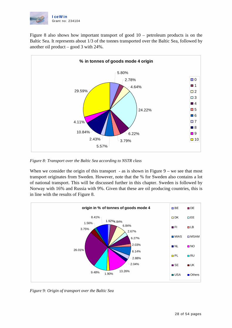
Figure 8 also shows how important transport of good 10 – petroleum products is on the Baltic Sea. It represents about 1/3 of the tonnes transported over the Baltic Sea, followed by another oil product – good 3 with 24%.
% in tonnes of goods mode 4 origin
5.80%
2.78%
4.64%
24.22%
6.22%
3.79%5.57%
2.43%
10.84%
4.11%
29.59%
012345678910
Figure 8: Transport over the Baltic Sea according to NSTR class
When we consider the origin of this transport - as is shown in Figure 9 – we see that most transport originates from Sweden. However, note that the % for Sweden also contains a lot of national transport. This will be discussed further in this chapter. Sweden is followed by Norway with 16% and Russia with 9%. Given that these are oil producing countries, this is in line with the results of Figure 8.
origin in % of tonnes of goods mode 4
1.92%4.84%6.84%
2.67%
6.27%
2.03%
6.14%
2.88%
2.04%
13.26%1.90%9.48%
26.01%
3.75%
1.56%
8.41%
BE DE
DK EE
FI LB
MIAS MSAM
NL NO
PL RU
SE UK
USA Others
Figure 9: Origin of transport over the Baltic Sea
28 of 54 pages

IceWin Grant no: 234104
In the remainder of this chapter, we focus on the import of goods in the EU member states of the different goods. The reason for this focus is that a disruption in import will have a larger effect on the economy of those countries than the disruption in their export. A lack of import will directly affect other sectors if inputs become scarce. A disruption in export might hinder the competitiveness of those countries as they might be seen as less reliable, but this cannot be modelled with a model like EDIP.
In the next sections we discuss imports into the 6 countries which would be hit the most if an interruption in traffic flows would take place, this is we discuss the EU member states Estonia, Finland, Lithuania, Latvia, Poland and Sweden.
4.1.1 Import into Estonia
76% of all imports into Estionia originates from the 10 countries mentioned above. Of course also other countries import to Estonia, and given the location of this country, this import will also travel over the Baltic Sea. 29% of all imports into Estonia happen via the Baltic Sea. As Table 3 shows, goods 1, 3, 5, 6 and 9 are relatively more imported via the Baltic Sea than via road or rail, etc.
Table 3: Share of import into Estonia via the Baltic Sea
Good 0 1 2 3 4 5 6 7 8 9 10 Grand Totalshare of import via the Baltic Sea 28% 48% 2% 44% 5% 37% 48% 0% 29% 39% 18% 29%
Figure 10 shows all import into Estonia in tons, divided according to NSTR classes. It is clear from this picture that goods 6 (22%), 9 (19%) and 1 (17%) are the goods with the highest share of import. Given that it is a neighbour of Russia, reachable over land, oil import over the Baltic Sea is less important.
Import into EE according to NSTR classes
13%
17%
0%
2%
1%
11%22%
0%
6%
19%
9%
012345678910
Figure 10: Import via the Baltic Sea into Estonia according to NSTR classes
29 of 54 pages

IceWin Grant no: 234104
4.1.2 Import into Finland
79% of all imports into Estionia originates from the 10 countries mentioned above. Most of the import originates from Russia – 27%. According to the data, only 11% of all imports into Finland happen via the Baltic Sea. Given its location, this seems rather low. Further analysis of the data showed that for the majority of the transport flows into Finland the mode is marked as ‘unknown’. Hence, the share of imports via the Baltic Sea is probably underestimated. Moreover, Russia is the main origin of import into Finland, and can be reached over land. According to the data, only 8% of Russians export into Finland happens via the sea and this gets a high weight. As Table 3 shows, mainly goods 10, 0, 2 and 7 are relatively more imported via the Baltic Sea than via road or rail, etc.
Table 4: Share of import into Finland via the Baltic Sea
Good 0 1 2 3 4 5 6 7 8 9 10 Grand Totashare of import via the Baltic Sea 14% 0% 11% 7% 3% 0% 0% 11% 10% 0% 38% 11%
Figure 10 shows all import into Finland in tons, divided according to NSTR classes. It is very clear from this picture that the oil products - goods 10 (42%), good 2 (12%), good 3 (10%) and good 0 (24%) are the goods with the highest share of import.
Import into Finland according to NSTR classes
24%
0%
10%
12%3%0%0%
1%
8%0%
42%
012345678910
Figure 11: Import via the Baltic Sea into Finland according to NSTR classes
4.1.3 Import into Lithuania
69% of all imports into Lithuania originates from the 10 countries mentioned above. Of good 2, 100% of all import originates from the 9 others, and of good 5, 99%. 13% of all imports into Lithuania happen via the Baltic Sea. As can be seen from the table below, goods 4 and 7 are more represented than the other goods. Given the pipeline connection between Russia and Lithuania, the relatively low share of oil products is logic.
Table 5: Share of import into Lithuania via the Baltic Sea
Good 0 1 2 3 4 5 6 7 8 9 10 Grand Totalshare of import via the Baltic Sea 3% 7% 0% 0% 22% 5% 9% 33% 0% 8% 2% 13%
30 of 54 pages

IceWin Grant no: 234104
Figure 12 shows all import into Lithuania in tons, divided according to NSTR classes. It is very clear from this picture that goods 7 (72%) is the good with the highest share of import. If there would be an interruption in transport over the Baltic Sea, sectors using this good as an input would be hit the most.
Import to LT via Baltic sea according to NSTR
3% 5%0%0%1%2%
10%
72%
0% 6%
1%
012345678910
Figure 12: Import via the Baltic Sea into Lithuania according to NSTR classes
4.1.4 Import into Latvia
61% of all imports into Latvia originates from the 10 countries mentioned above. 34% of all imports into Latvia happen via the Baltic Sea. As Table 6 shows, for some goods such as 2,4,7 and 8, the majority of the import happens via the Baltic Sea. The relatively lower share in general is explained by the lower % for good 6, which is very important in absolute terms.
Table 6: Share of import into Latvia via the Baltic Sea
Good 0 1 2 3 4 5 6 7 8 9 10 Grand Totashare of import via the Baltic Sea 66% 55% 98% 46% 98% 65% 17% 98% 83% 51% 23% 34%
l
Figure 13 shows all import into Latvia in tons, divided according to NSTR classes. It is clear from this picture that goods 9 (49%) and 8 (18%) are the goods with the highest share of import. As in Lithuania, the shares for the oil products are relatively low as there is also a pipeline connection between Russia and Latvia.
31 of 54 pages
IceWin Grant no: 234104
import into LV via baltic sea in nstr
3%14%
0%
0%
0%
5%
1%
1%
18%50%
8% 012345678910
Figure 13: Import via the Baltic Sea into Estonia according to NSTR classes
4.1.5 Import into Poland
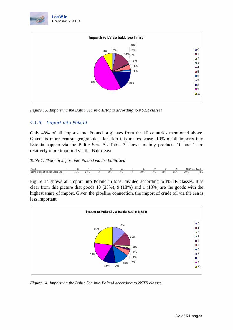
Only 48% of all imports into Poland originates from the 10 countries mentioned above. Given its more central geographical location this makes sense. 10% of all imports into Estonia happen via the Baltic Sea. As Table 7 shows, mainly products 10 and 1 are relatively more imported via the Baltic Sea
Table 7: Share of import into Poland via the Baltic Sea
Good 0 1 2 3 4 5 6 7 8 9 10 Grand Totshare of import via the Baltic Sea 11% 21% 5% 2% 1% 7% 10% 1% 10% 11% 30% 10%
al
Figure 14 shows all import into Poland in tons, divided according to NSTR classes. It is clear from this picture that goods 10 (23%), 9 (18%) and 1 (13%) are the goods with the highest share of import. Given the pipeline connection, the import of crude oil via the sea is less important.
import to Poland via Baltic Sea in NSTR
12%
13%
2%
1%
1%
5%13%0%11%
18%
23%
012345678910
Figure 14: Import via the Baltic Sea into Poland according to NSTR classes
32 of 54 pages

IceWin Grant no: 234104
4.1.6 Import into Sweden
77% of all imports into Sweden originates from the 10 countries mentioned above. However, if we remove Sweden from the countries of origin, only 45% of all imports originates from the other 9 countries. This shows the importance of maritime transport from Sweden to Sweden. In total, 4% of all transport from Sweden to Sweden happens via the Baltic Sea. This makes that if shipping on the Baltic Sea would be interrupted, not only import from other countries would be hindered, but also national transport flows.
39% of all imports into Sweden – including transport originating from Sweden - happen via the Baltic Sea. As Table 8 shows, mainly oil goods 10, 2 and 3 and good 4 are well represented. 32% of this transport is transport from Sweden to Sweden and mainly good 10 (95%) and good 4 (30%) are shipped inside Sweden.
Table 8: Share of import into Sweden via the Baltic Sea
Good 0 1 2 3 4 5 6 7 8 9 10 Grand Totalshare of import via the Baltic Sea 2% 1% 39% 53% 83% 31% 16% 20% 44% 5% 87% 39%
Figure 15 shows all import into Sweden – including the own transport - in tons, divided according to NSTR classes. Goods 3 (35%), 10 (31%) have the highest share between the goods transported via the Baltic Sea.
import into Sweden via Baltic Sea in NSTR1%
0%
4%
35%
8%4%3%
1%
12%
1%
31%
012345678910
Figure 15: Import via the Baltic Sea into Sweden according to NSTR classes
4.2 Of oil goods
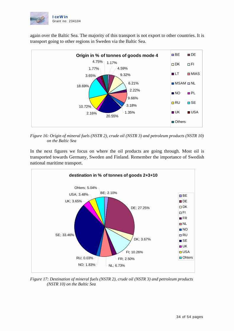
In this section we focus on the mineral fuels (NSTR 2), crude oil (NSTR 3) and petroleum products (NSTR 10). Of all oil products travelling over the Baltic Sea, the majority (20.55%) originates from Norway, followed by Sweden (18.69%) and Russia (10.72%). At first sight the high share of Sweden seems odd, as Sweden is not an oil producing country. However, remember the relatively high share of national maritime transport. When we look further, we see that of all oil products exported by Sweden, 97.5% are petroleum products. Hence, what we see is how crude oil is imported in Sweden, refined and then transported
33 of 54 pages
IceWin Grant no: 234104
again over the Baltic Sea. The majority of this transport is not export to other countries. It is transport going to other regions in Sweden via the Baltic Sea.
Origin in % of tonnes of goods mode 4
9.32%
6.21%
2.22%
9.66%
3.18%
1.35%20.55%
2.16%
10.72%
18.69%
3.65%
1.77%
4.75% 1.17%4.59%
BE DE
DK FI
LT MIAS
MSAM NL
NO PL
RU SE
UK USA
Others
Figure 16: Origin of mineral fuels (NSTR 2), crude oil (NSTR 3) and petroleum products (NSTR 10) on the Baltic Sea
In the next figures we focus on where the oil products are going through. Most oil is transported towards Germany, Sweden and Finland. Remember the importance of Swedish national maritime transport.
destination in % of tonnes of goods 2+3+10
BE; 2.10%
DE; 27.25%
DK; 3.67%
FI; 10.26%
FR; 2.50%
NL; 6.73%NO; 1.83%
RU; 0.03%
SE; 33.46%
UK; 3.65%
USA; 3.48%
Ohters; 5.04%
BEDEDKFIFRNLNORUSEUKUSAOhters
Figure 17: Destination of mineral fuels (NSTR 2), crude oil (NSTR 3) and petroleum products
(NSTR 10) on the Baltic Sea
34 of 54 pages

IceWin Grant no: 234104
5 What could be the effect of interruptions in transport over the Baltic Sea
In this final chapter we discuss qualitatively the possible effect of interruptions in transport over the Baltic Sea. We discuss separately the effect of a possible interruption in oil supply and an interruption in the supply of other goods. Finally, we make the link with how this could be modelled using the EDIP model.
5.1 Interruptions in oil supply
The analysis in previous chapters showed that in order to know the effect of disruptions in oil supply we need to know the importance of the oil originating from the Baltic Sea and the alternatives. Notwithstanding national differences, for the EU as a whole about 30% of the oil consumed originates from Russia. About 30% is shipped over the Baltic Sea to other European countries. Hence, at most around 10% of the average EU oil supply could be interrupted because of a combination of a freezing of the Baltic Sea and insufficient ice breaking resources. For countries around the Baltic Sea, not connected with a pipeline with Russia, this share would be much larger.
If an oil interruption would happen, there are two possible solutions. Either one tries to find an alternative source or one relies on the national oil reserves. For Sweden, using an alternative source could proof difficult as the other oil producing European countries such as Denmark and Norway are also situated around the Baltic Sea. For a country like Finland land transport via Russia could be a solution. For other countries such as Poland and Germany, an increase in transport via pipelines would be a valid alternative. The use of the reserves should be feasible for all countries. Most countries have enough resources to last for a reasonable long period. However, there are some questions for countries using a ticket system and for countries where the stocks are actually held by the industry. Also, demand is increasing over time, not only in Europe, so in the future there might be less spare capacity.
The final question remains: what is the probability of an oil supply interruptions. This depends on the evolution in climate, the changes icebreaking resources, and whether oil transport would be prioritized or not. In summary, this first analysis leads to the conclusion that oil interruptions might not be a major problem. However, this conclusion should be treated with care as there are still a lot of unknowns.
5.2 Interruptions in import of other goods
As oil supply interruptions might not be a major problem, we decided to extend the analysis to other goods as well. Interruptions in export of goods might lead to problems of competitiveness for the countries around the Baltic Sea as it decreases their reliability. However, this is hard to determine quantitatively. Therefore we focus on the effect of
35 of 54 pages

IceWin Grant no: 234104
disruptions in import of goods on the economies of the countries around the Baltic Sea. The effect of such interruptions will depend on
- relative importance of import of goods in national production
- available stock
- length of the interruption
The effect is less pronounced than for oil. Hence, we need a model capturing all this information to analyse the effects.
5.3 Link with EDIP
The European Model for the Assessment of Environmental, Economic and Social effects of Sustainability Policies (EDIP) is described in detail in annex 1. The EDIP model is a dynamic, recursive over time, model, involving dynamics of capital accumulation and technology progress, stock and flow relationships and backward looking expectations. It includes the representation of the micro-economic behaviour of the following economic agents: several types of households differentiated by 5 income quintiles, 3 degrees of urbanization and 6 family types; production sectors differentiated by 59 NACE classification categories; investment agent; federal government and external trade sector.
EDIP includes detailed representation of the production technology of all major energy sectors as well as the complex substitution possibilities between different energy inputs. It also includes distinction between income classes, family types and education levels, which make the model applicable for assessment with social indicators in a quantitative way.
Important for the analysis of supply disruptions is the fact that the EDIP model builds on a social accounting matrix which captures 59 industries, denoted by their NACE coding. Industry 5 captures the ‘crude petroleum and natural gas; services incidental to oil and gas extraction excluding surveying’ and industry 23 captures the ‘coke, refined petroleum products and nuclear fuels’.
This means that within task 3.3 – the assessment of the effects, we will need to disaggregate these sectors in order to isolate the effect of oil supply disruptions. Furhtermore, we need to make a link between the ETIS data – only distinguishing between 11 types of goods and the 59 products within EDIP.
In practice, there are two ways of modelling a supply disruption: either via a price increase or via an actual stop in supply.
5.3.1 A price increase
In the literature, the effect a supply disruption in oil has often been modelled as the effect of a sudden price increase. The idea is that a supply disruption would lead to an increase in the price as the good becomes more scarce, rather than that the supply would actually come to a
36 of 54 pages

IceWin Grant no: 234104
halt. In the IEA's world energy outlook 2005 it is stated that a 10$ price increase of oil leads to cut in GDP in OECD countries by 0.4%. The EC (2008) found that an increase in oil prices of 100% over a period of 3 years would decrease GDP by 0.9% below the baseline after three years. This loss is unevenly spread over the sectors. According to the model used, the impact on consumption is stronger: 2% lower after 3 years as consumer prices are 2% higher after 3 years. Further analysis showed that the effect of an increase in oil prices is non linear - the higher the initial price level, the higher the effect of a price increase. This implies that a price increase would have a higher effect than fuel shortage.
Using this methodology also requires the estimation of the effect of the supply disruption on the price. Given the complexity of the oil market as a whole, this would require a lot of detailed information – information which is not readily available.
5.3.2 Actual stop of supply
An alternative would be to actually stop the supply of a good within EDIP. Given its recursive nature, this could be done for a week, a month, a year. This method requires much less information as it does not require to answer questions like: are there alternative sources, can the reserves be actually used, what would be the effect on the prices, etc. This benefit is also the greatest drawback as it would be more a representation of the worst case scenario than an actual representation of what would happen in reality.
37 of 54 pages
IceWin Grant no: 234104
References Borisocheva, K. (2007), Analysis of the Oil-and Gas-Pipeline-Links between EU and Russia – An account of intristic interests, CERE
EIA Website, Russia Oil exports http://www.eia.doe.gov/emeu/cabs/Russia/OilExports.html
Energy pocket book (2009), http://ec.europa.eu/energy/publications/statistics/statistics_en.htm
ETIS-BASE website: http://www.iccr-international.org/etis/base/index.html
European Commission (2007), The Northern Transit Axis, Final Report, November 2007, European Commission, Directorate-General Energy and Transports
European Commission, REGISTRATION OF CRUDE OIL IMPORTS AND DELIVERIES IN THE COMMUNITY, http://ec.europa.eu/energy/observatory/oil/doc/import/2005_cce_eu25.xls
European Commission (2008), Commission Staff Working Document, accompanying document to the Proposal for a Directive of the Council Imposing an obligation on Member States to maintain minimum stocks of crude oil and/or petroleum products – Impact Assessment.
European Commission (2009), http://europa.eu/rapid/pressReleasesAction.do?reference=IP/09/1718&language=en
European Commission (2010), http://ec.europa.eu/energy/observatory/oil/stocks_en.htm
Eurostat (2009), EU27 Trade Since 1995 By BEC
EX-TREMIS project : http://www.ex-tremis.eu/about.htm
HELCOM Stakeholder Conference on the Baltic Sea Action Plan (2006), Maritime transport in the Baltic Sea. Draft HELCOM Thematic Assessment, 7 March 2006
Ivanova O., De Ceuster G., Chen M., Tavasszy L., April 2007: Deliverable 4.2: Assessing transport policy impacts on transport safety, on equity and on income distribution
US Energy Information Administration, International Energy Statistics, Total Oil Supply, http://tonto.eia.doe.gov/cfapps/ipdbproject/IEDIndex3.cfm?tid=5&pid=53&aid=1
US Energy Information Administration, International Energy Statistics, Total Consumption of Petroleum Products, http://tonto.eia.doe.gov/cfapps/ipdbproject/IEDIndex3.cfm?tid=5&pid=54&aid=2
38 of 54 pages
IceWin Grant no: 234104
1 Annex 1: Description of the EDIP model.
This annex describes the construction the European Model for the Assessment of Environmental, Economic and Social effects of Sustainability Policies (EDIP). The model is constructed using the Computable General Equilibrium (CGE) framework, which takes as a basis the notion of the Walrasian equilibrium.
The EDIP model is a dynamic, recursive over time, model, involving dynamics of capital accumulation and technology progress, stock and flow relationships and backward looking expectations. It includes the representation of the micro-economic behaviour of the following economic agents: several types of households differentiated by 5 income quintiles, 3 degrees of urbanization and 6 family types; production sectors differentiated by 59 NACE classification categories; investment agent; federal government and external trade sector.
EDIP includes detailed representation of the production technology of all major energy sectors as well as the complex substitution possibilities between different energy inputs. It also includes distinction between income classes, family types and education levels, which make the model applicable for assessment with social indicators in a quantitative way.
The first version of the model has been applied to the estimation of the temporal economic, environmental and social effects of the energy taxation as described in the EU Energy Taxation Directive.
1.1 Introduction
The EDIP model was constructed within the REFIT project (FP6-022578). With this research, we want to develop, test and validate a modelling tool that produces data on a set of identified indicators and that enables ex-ante evaluation of transport and energy policy considering the economic, environmental and, which is new in economic modelling, social dimensions of sustainability. Up until now, modelling tools covered very well the economic and environmental dimension, with this model we want to include the social dimension of sustainability in policy assessment.
In almost every recent paper on sustainable transport there is a statement about the underdeveloped "poor-relation", social dimension and lacking knowledge about the social aspects of sustainability. This is partly due to the fact that a lot of social indicators overlap with economical and environmental indicators. We will make a step forward in addressing the impacts of transport policy on equity & income distribution. This aspect considers the allocation of costs between different income classes. This indicator is used to justify efforts to keep transport costs “affordable” to disadvantaged lower-income transport system users.
The primary aim of the socio-economic model called European Model for the Assessment of Environmental, Economic and Social effects of Sustainability Policies (EDIP) is to assess the inequality and income distribution effects of the energy and transport related
39 of 54 pages

IceWin Grant no: 234104
policies. The model focuses on the socio-economic aspects of the policy effects. It includes detailed representation of the household types as well as the detailed representation of the types of individuals. Given such detailed representation of the population structure, the EDIP model is able to incorporate a thorough modelling of the labour market and unemployment. It also includes the national-level wage bargaining for each of the NACE95 sectors.
1.1.1 State-of-the-art
The detailed structure of the labour market and representation of the different socio-economic groups is the feature that differentiates the EDIP model from all other existing state-of-the-art modelling tools. This feature makes it better suited for the assessment of socio-economic effects of various policies than other existing models.
EDIP is the first European-wide model to include detailed search and matching formulation of labor market, a realistic representation of wage formation via bargaining mechanism and unemployment per education level and occupation type. This distinctive feature of the model makes it well-suited for the assessment of detailed unemployment effects of governmental polices. It can also assess the policy impacts on the wage levels of various labor types.
Given that EDIP is a general equilibrium model, it incorporates the full representation of production and consumption activities in the economy. The model has rather refined representation of production technologies of the sectors and detailed sector/commodity disaggregation, which is consistent with EuroStat NACE95 classification. EDIP treats energy substitution possibilities of the sectors and households in a realistic way. In its energy part the model borrows from the best international state-of-the-art practices in modeling.
Households’ welfare in the EDIP model is negatively influenced by the amount of emissions associated with production and consumption activities in the country, where a certain share of emissions is allocated to different household types. EDIP is the first European model, which allocates emissions differently between the income groups. The allocation rule depends upon the type of the pollutant. In case of the regional pollutants, a larger share is allocated to the poor household groups.
The core of the own-production part of the model is the modeling of the joint demand for durable and non-durable goods. Modeling of the durables and non-durables link in EDIP is similar to the one used in GEM-E3.
1.1.2 Model overview
The EDIP model is constructed using the Computable General Equilibrium (CGE) framework, which takes as a basis the notion of the Walrasian equilibrium.
40 of 54 pages

IceWin Grant no: 234104
CGE models are a class of economic models that use actual economic data to estimate how an economy might react to changes in policy, technology or other external factors. A model consists of (a) equations describing model variables and (b) a database (usually very detailed) consistent with the model equations. The EDIP model is based on the social, economic, environmental transport and energy data for the year 2005. The EDIP database covers EU27 countries, Norway, Switzerland, Croatia and Turkey.
The model equations tend to be neo-classical in spirit, assuming cost-minimizing behavior by producers, average-cost pricing, and household demands based on optimizing behavior. A CGE model database consists of tables of transaction values and elasticities: dimensionless parameters that capture behavioral response. The database is presented as a social accounting matrix (SAM). It covers the whole economy of a country, and distinguishes a number of sectors, commodities, primary factors and types of households.
Behavior of the households is based on the utility-maximization principle. Household’s utility is associated with the level and structure of its consumption. Each household spends its consumption budget on services and goods in order to maximize its satisfaction from the chosen consumption bundle. Utility of the household is maximized under the budget constraint. Households in the EDIP model receive their income in the form of wages, capital rent, unemployment benefits and other transfers from the federal government.
Behavior of the sectors is based on the minimization of the production costs for a given output level under the sector’s technological constraint. Production costs of each sector in the EDIP model include labor costs by type of labor, capital costs and the costs of intermediate inputs. The sector’s technological constraint describes the production technology of each sector. In accordance with their production technology, sectors have substitution possibilities between different intermediate inputs and production factors. They can substitute between the use of different education types and between different occupations within each education type. They are also able to substitute between their consumption of electricity and other energy types such as gas, coal and refined oil.
An Armington assumption on international trade is adopted in the model. According to this assumption the commodities produced by the domestic sectors for the consumption inside the country and for the consumption outside of it have different specifications. Domestic sales of each of the 59 types of commodities composed of the commodities produced by the domestic sectors, those imported from the EU25 and those imported from the rest of the world. According to the Armington assumption, the same type of commodity produced by the domestic sectors, imported from the EU25 or imported from the rest of the world has different specifications and, hence, cannot be treated as a homogenous good.
The model incorporates the representation of investment and savings decisions of the economic agents. Savings in the economy are made by households, government and the rest of the world. The total savings accumulated at each period of time are invested into accumulation of the sector-specific physical capital, which is not mobile between the sectors. The stock of this capital at each period of time is equal to the last period stock minus depreciation plus the new capital accumulated during the previous period of time.
41 of 54 pages

IceWin Grant no: 234104
The EDIP model incorporates the representation of the federal government. The governmental sector collects taxes, pays subsidies and makes transfers to households, production sectors and to the rest of the world. The federal government consumes a number of commodities, where the optimal governmental demand is determined according to the maximization of the governmental consumption utility function. The model incorporates the governmental budget constraint. According to this constraint the total governmental tax revenues are spend on subsidies, transfers, governmental savings and consumption.
Finally, the model includes the trade balance constraint, according to which the value of the country’s exports plus the governmental transfers to the rest of the world are equal to the value of the country’s imports.
1.1.3 Applicability
Thorough sectoral disaggregation of the EDIP model allows one to assess sector-specific impacts of the transport and energy policies in great detail and provides its users with useful insights into the channels, through which policy measures influence the economies of the European countries.
Besides the representation of the transport-related taxes, the EDIP model also includes all other major taxes and subsidies in the economy. It represents both the governmental spending and governmental budget in detail. Governmental spending includes its transfers to different income quintiles besides other things. This particular model feature makes it possible for the user to assess the combined effect of measures, related to different policy areas. For example, it allows one to combine an increase in the fuel tax with higher governmental transfers to poor income groups. The model user can analyze not only in which way it is the best to collect transport and energy-related revenues but also in which way it is the best to spend them.
The EDIP model is well suited for the assessment of a wide range of energy, transport, economic and social policies. The model allows for the calculation of broad welfare and macro-economic effects of the policies as well as their sector-specific and labor market effects.
The model can help with an evaluation of both separate measures and packages of policies. Despite its broad nature, the main focus of the EDIP model is an assessment of impact of transport-related policies on inequality and income distribution in the economies of European countries.
1.2 The EDIP Model structure
The EDIP model has a single mathematical formulation for all European countries. It is one model with 31 different versions, which are estimated using the country-specific dataset. The main element of the country-specific dataset of the EDIP model is the Social Accounting Matrix (SAM), which represents the annual monetary flows between different economic agents for the year 2005. Structure of the SAMs does not differ between the
42 of 54 pages

IceWin Grant no: 234104
countries and corresponds to the overall structure of the EDIP model. Other country-specific data includes the socio-economic data related to different household types, labor market data, transport data, energy and emissions data. The EDIP model uses the latest available data from different statistical sources including EuroStat, national statistical offices, International Labor Organization, OECD, IEA etc.
CGE models utilize the notion of the aggregate economic agent. They represent the behavior of the whole population group or of the whole industrial sector as the behavior of one single aggregate agent. It is further assumed that the behavior of each such aggregate agent is driven by certain optimization criteria such as maximization of utility or minimization of costs.
The EDIP model includes the representation of the micro-economic behavior of the following economic agents: several types of households differentiated by 5 income quintiles, production sectors differentiated by 59 NACE classification categories; investment agent; federal government and external trade sector. Each household group in the EDIP model consists of the individuals differentiated by three types of education levels and ten types of professions. The composition of households is based on the extensive socio-economic dataset for the year 2005.
The EDIP model is a dynamic, recursive over time, model, involving dynamics of capital accumulation and technology progress, stock and flow relationships and backward looking expectations. A recursive dynamic structure composed of a sequence of several temporary equilibriums. The first equilibrium in the sequence is given by the benchmark year. In each time period, the model is solved for an equilibrium given the exogenous conditions assumed for that particular period. The equilibriums are connected to each other through capital accumulation. Thus, the endogenous determination of investment behavior is essential for the dynamic part of the model. Investment and capital accumulation in year t depend on expected rates of return for year t+1, which are determined by actual returns on capital in year t.
Apart from the model description in this annex, a full mathematical formulation of the model can be found in online reports on http://www.refitweb.eu/
1.2.1 Production
Behaviour of the sectors is based on the minimization of the production costs for a given output level under the sector’s technological constraint. Production costs of each sector in the EDIP model include labour costs by type of labour, capital costs and the costs of intermediate inputs. The sector’s technological constraint describes the production technology of each sector. It provides information on how many of different units of labour, capital and of the 59 commodities, traded in the economy, are necessary for the production of one unit of the composite sectoral output.
Production technology of the sectors in EDIP is represented using a Constant Elasticity of Substitution (CES) function. Substitution possibilities at each of the nests are captured by
43 of 54 pages

IceWin Grant no: 234104
the corresponding elasticity of substitution parameter. The higher the values of this parameter the easier it is to substitute between the inputs. The intermediate demands of the firms are determined by the relative prices of commodities and the substitution possibilities between them, which are summarized in the form of the CES tree (Figure 1).
At the top level of the production function, the firms use the capital-labour-energy bundle, the composite transport bundle and other intermediate inputs in fixed proportion to the total composite output. At the level of the capital-labour-energy bundle, the firms can substitute between the use of the composite energy bundle and the capital-labour bundle. In case of the energy inputs, the sector can further substitute between electricity and other energy, where other energy bundle includes coal, gas, oil and refined oil. The firms have possibility to substitute between the non-electric energy inputs.
At the level of the capital-labour bundle, the firms substitute between physical capital (such as machinery and buildings) and the composite labour input. For most of the sectors this substitution possibilities are rather limited. The composite labour is further split between the three educations levels, which are further subdivided into ten occupation types. The firms have the possibility to substitute between the education levels as well as between the occupation types. However, this possibility is limited.
At the level of the composite transport inputs, the firms can substitute between the two distance classes of their trips: below 500 km and above 500 km. The length of the trip strongly influences the choice of the transportation mode used to perform the trip. The two distance classes of transportation are further split between the transportation by different modes including land, air and water. Transportation by air and water are produced by the respective production sectors and are bought by the firms.
Transportation by land is treated differently. It can be either purchased from the land transport sector or produced by the firms themselves. Own-production of land transportation by the firms involves consumption of durables and non-durables bundle that is vehicles and maintenance and refined oil. In order to model the joint consumption of durables and non-durables we have split the total inputs of maintenance and refined oil into the minimum/fixed amount necessary for the use of a vehicle and the rest. The minimum/fixed amount of the inputs of refined oil and maintenance is associated with the fact of having a vehicle. The rest part of the inputs of refined oil and maintenance is associated with driving more with the same vehicle.
44 of 54 pages
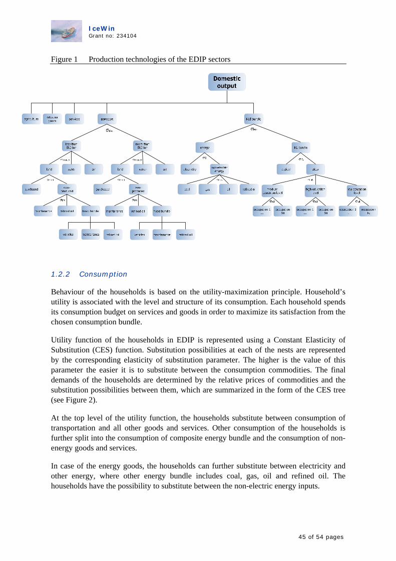
IceWin Grant no: 234104
Figure 1 Production technologies of the EDIP sectors
1.2.2 Consumption
Behaviour of the households is based on the utility-maximization principle. Household’s utility is associated with the level and structure of its consumption. Each household spends its consumption budget on services and goods in order to maximize its satisfaction from the chosen consumption bundle.
Utility function of the households in EDIP is represented using a Constant Elasticity of Substitution (CES) function. Substitution possibilities at each of the nests are represented by the corresponding elasticity of substitution parameter. The higher is the value of this parameter the easier it is to substitute between the consumption commodities. The final demands of the households are determined by the relative prices of commodities and the substitution possibilities between them, which are summarized in the form of the CES tree (see Figure 2).
At the top level of the utility function, the households substitute between consumption of transportation and all other goods and services. Other consumption of the households is further split into the consumption of composite energy bundle and the consumption of non-energy goods and services.
In case of the energy goods, the households can further substitute between electricity and other energy, where other energy bundle includes coal, gas, oil and refined oil. The households have the possibility to substitute between the non-electric energy inputs.
45 of 54 pages

IceWin Grant no: 234104
At the level of the composite transport bundle, the households can substitute between the two distance classes of their trips: below 500 km and above 500 km. The length of the trip strongly influences the choice of the transportation mode used to perform the trip. The two distance classes of transportation are further split between the transportation by different modes including land, air and water. Transportation by air and water are produced by the respective production sectors and are bought by the firms.
Transportation by land is treated differently. It can be either purchased from the land transport sector or produced by the households themselves. Own-production of land transportation by the households involves consumption of durables and non-durables bundle that is vehicles and maintenance and refined oil. In order to model the joint consumption of durables and non-durables we have split the total inputs of maintenance and refined oil into the minimum/fixed amount necessary for the use of a vehicle and the rest. The minimum/fixed amount of the inputs of refined oil and maintenance is associated with the fact of having a vehicle. The rest part of the inputs of refined oil and maintenance is associated with driving more with the same vehicle.
Figure 2 Structure of the households’ utility
Utility of the household is maximized under the budget constraint, where the household’s consumption spending is equal to its income minus income tax and the household’s savings. Households in the EDIP model receive their income in the form of labour income, capital rent, unemployment benefits and other transfers from the federal government. Labour income of the households consists of wages received from different production
46 of 54 pages

IceWin Grant no: 234104
sectors. The labour compensation differs between the three education levels and ten occupation types. The structure of the households’ income is represented in Figure 3.
Figure 3 Structure and sources of the households’ income
The level of the unemployment benefits, received by the household, depends upon the level of unemployment associated with the particular education level and occupation type of the individuals within the household. The level of the unemployment for each education-occupation bundle is defined according to the search and matching model by Pissaridi and depends upon the mismatch upon the available labour and available vacancies.
1.2.3 Transport sector
Households and domestic sectors use transport services in their consumption and production activities. The transport services represented in the EDIP model are differentiated by the two distance classes (below 500km and above 500km) and all main types of transport modes (land, water and air). Each type of transport service is associated with the particular after tax price, which includes VAT taxes and other taxes.
47 of 54 pages
IceWin Grant no: 234104
Public transport and freight transport services are produced by several national transport sectors. These sectors use labor, capital and commodities, for example fuels and vehicles, as inputs to their production. The price of transportation services are determined endogenously in the EDIP model according to the equilibrium condition of the transportation markets.
Passenger transportation by car is produced by the households and firms themselves using fuel and car vehicles. In order to have a passenger car vehicle a household has to pay the car ownership costs, which include different types of taxes, such as registration taxes, for example.
The EDIP model employs the concept of a variable expenditure function with quasi-fixed durable goods (car vehicles) as arguments in order to derive a demand system for nondurable goods (fuels) in prices of the nondurables, in the stocks of durables and in variables expenditure. Investment demand for durables and their desired stocks (car stocks) are determined inside the model. The desired stock of cars in the EDIP model depends upon the development of the demand for transportation and the car ownership costs.
1.2.4 International trade
Each sector in the economy may produce more then one type of commodity and the combination of these different commodities corresponds to the sectoral composite output. Production output of each sector can be either delivered to the domestic market or exported to EU25 trade zone or to the rest of the world. Each sector determines the shares of its outputs sold domestically and exported based on the profit maximization principle. It takes into account the relative prices of the same type of commodities in its own country and abroad.
An Armington assumption on international trade is adopted in the model. According to this assumption the commodities produced by the domestic sectors for the consumption inside the country and for the consumption outside of it have different specifications. In order for the sector to be able to switch its technological process between producing these two different specifications of commodities, it has to overcome some adjustments.
The degree of difficulty and feasibility of such adjustment is represented by the constant elasticity of transformation (CET) elasticity of substitution between producing commodity for the domestic use, for export to the EU25 and for the export to the rest of the world. The higher is this elasticity of substitution the more feasibly and easy the adjustment technological process described above. Than the proportions, in which the total output of each sector is split between the three possibilities, depend not only upon the relative prices of the commodities inside the country and on the world market but also upon the CET elasticity of substitution (see Figure 4).
48 of 54 pages

IceWin Grant no: 234104
Figure 4 CET function for the representation of export decisions of domestic sectors
Domestic sales of each of the 59 types of commodities composed of the commodities produced by the domestic sectors, those imported from the EU25 and those imported from the rest of the world. According to the Armington assumption, the same type of commodity produced by the domestic sectors, imported from the EU25 or imported from the rest of the world has different specifications and, hence, cannot be treated as a homogenous good. Domestic consumers have different preferences for these three specifications and can substitute between them in case the relative prices of the specifications change. The substitution possibilities between these three commodity specifications are represented by the Armington elasticity of substitution and vary between the types of commodities. The shares in which commodity is bought from the domestic producers, from the EU25 and from the rest of the world are determine by the relative producer prices of the commodity inside the country, in EU25 and in the rest of the world as well as by the Armington elasticity of substitution (see Figure 5).
Figure 5 CES function for the representation of international trade
Finally, the model includes the trade balance constraint, according to which the value of the country’s exports plus the governmental transfers to the rest of the world are equal to the value of the country’s imports.
49 of 54 pages

IceWin Grant no: 234104
1.2.5 Labour market
The unemployment in the EDIP is modelled according to the search-and-matching approach, which explains the existence of frictional unemployment in the country. The main idea behind this approach is that there exists a mismatch between the available vacancies and the unemployed labour. It takes firms and individuals some time to find the right vacancy/employee, which results in the frictional unemployment. The level of this type of unemployment varies between the education types and occupations (see Table 1).
• N0
in EDIP
• Isced-97 classification
• Full name of education type
• 1 • isced0_2 • Pre-primary, primary and lower secondary education - levels 0-2 (ISCED 1997)
• 2 • isced3_4 • Upper secondary and post-secondary non-tertiary education - levels 3-4 (ISCED 1997)
• 3 • isced5_6 • Tertiary education - levels 5-6 (ISCED 1997)
• N0
in EDIP
• ISCO-88 classification
• Full name of occupations
• 1 • isco1
• Legislators, senior officials and managers
• 2 • isco2 • Professionals
• 3 • isco3
• Technicians and associate professionals
• 4 • isco4 • Clerks
• 5 • isco5
• Service workers and shop and market sales workers
• 6 • isco6
• Skilled agricultural and fishery workers
• 7 • isco7 • Craft and related trades workers
50 of 54 pages

IceWin Grant no: 234104
• 8 • isco8
• Plant and machine operators and assemblers
• 9 • isco9 • Elementary occupations
• 10 • isco0 • Armed forces
Table 1 Education levels and occupations used in EDIP
The levels of the wages earned in different sectors of the economy by individuals with different education levels and occupation types are determined by the national-level bargaining process between the sector-specific trade union and the firms. Firms share partially their profits with their employees by paying them wages, which are higher then their marginal product of labor.
1.2.6 General equilibrium structure
The EDIP model is formulated and solved as a mixed complementarity problem (MCP), where three inequalities should be satisfied: the zero profit, market clearance, and income balance conditions. Using the MCP approach, a set of three non-negative variables is involved: prices, quantities, and income levels.
The zero profit condition requires that any activity operated at a positive intensity must earn zero profit (i.e., value of inputs must be equal or greater than value of outputs). Activity levels y for constant returns to scale production sectors are the associated variables with this condition. It means that either y > 0 (a positive amount of y is produced) and profit is zero, or profit is negative and y = 0 (no production activity takes place).
The market clearance condition requires that any good with a positive price must have a balance between supply and demand and any good in excess supply must have a zero price. Price vector p (which includes prices of final goods, intermediate goods and factors of production) is the associated variable.
The income balance condition requires that for each agent (including any government entities) the value of income must equal the value of factor endowments and tax revenue.
A characteristic of the CES production and consumption structures that are used throughout the model is that all inputs (consumption goods) are necessary inputs. Thus, for most markets the above conditions are satisfied with prices, output, income, and consumption of all goods strictly greater than zero, and with supply strictly equal to demand. Falling demand for an input or consumption good will simply mean that the price will fall very low.
Due to the existence of unemployment and wage bargaining on the labour market, it is in disequilibrium. The level of the wages is determined by the bargaining process between the trade unions and firms. It depends positively upon the probability to find a new job and the firms’ profits.
51 of 54 pages

IceWin Grant no: 234104
1.2.7 Government and its policy instruments
The EDIP model incorporates the representation of the federal government. The governmental sector collects taxes, pays subsidies and makes transfers to households, production sectors and to the rest of the world. The federal government consumes a number of commodities, where the optimal governmental demand is determined according to the maximization of the governmental consumption utility function. The model incorporates the governmental budget constraint. According to this constraint the total governmental tax revenues are spend on subsidies, transfers, governmental savings and consumption.
Figure 6 Schematic representation of government’s incomes and expenditures
Figure 6 summarizes the sources of income and nature of expenditures of the federal government. On the income side, the government receives taxes on production, consumption and incomes paid by firms and households. It also received all transport-related taxes. Besides the tax revenues, the federal government also acquires the monetary transfers from EU25 countries and from the rest of the world.
The total budget of the federal government is spent on subsidies to production and consumption, savings, transfers to the domestic households and to abroad. A part of the federal government’s budget is also spent on buying different commodities. These purchases are used by the government in order to provide certain services to the population of the country. Demands for these commodities are set such as to maximize the government’s consumption utility function. This utility function has a Cobb-Douglas functional form.
52 of 54 pages

IceWin Grant no: 234104
1.2.8 Emissions
All production and consumption activities in the EDIP model are associated with emissions and environmental damage. This is in particular true for the transportation. The model incorporates the representation of all major greenhouse gas and non greenhouse gas emissions. Emissions in the EDIP model are associated either with the use of different energy types by firms and households or with the overall level of the firms’ outputs.
The EDIP model incorporates all major types of greenhouse and non-greenhouse gas emissions. In particular it models the following types of emissions: CH4, CO, CO2, HCF, N2O, NMVOC, Nox, PFC, PM25, SF6 and SO2.
Emissions in EDIP are modeled as the fixed shares of either production inputs, production outputs of households’ consumption. The overall amount of emissions in the economy is equal to emissions of the households and emissions of the firms.
Each emission type represented in the model is associated with the monetary value. The monetary values of emissions are used to calculate the welfare changes for different households types, where the environmental quality is incorporate into the households’ welfare in a separable way.
1.2.9 Recursive dynamics
The model incorporates the representation of investment and savings decisions of the economic agents. Savings in the economy are made by households, government and the rest of the world. The total savings accumulated at each period of time are invested into accumulation of the sector-specific physical capital, which is not mobile between the sectors. The stock of this capital at each period of time is equal to the last period stock minus depreciation plus the new capital accumulated during the previous period of time.
The total investment into the sector-specific capital stock is spent on buying different types of capital goods such as machinery, equipment and buildings. The concrete mixture of different capital goods used for physical investments is determined by the maximization of the utility of the investment agent. This is an artificial national economic agent responsible for buying capital goods for physical investments in all the domestic sectors.
The EDIP model has a recursive dynamic structure composed of a sequence of several temporary equilibriums. The first equilibrium in the sequence is given by the benchmark year 2000. In each time period, the model is solved for an equilibrium given the exogenous conditions assumed for that particular period. The equilibriums are connected to each other through capital accumulation. In the benchmark case, we assume that the economy is on a steady-state growth path, where all the quantity variables grow at the same rate and all relative prices remain unchanged. When a policy measure is implemented the economy enters on a transition path, until, after some time it has reached a new steady-state growth path (Ballard, Fullerton, Shoven and Walley, 1985). We are of course interested in the
53 of 54 pages
IceWin Grant no: 234104
transition path induced by the policy measure and the characteristics of the new growth path.
The endogenous determination of investment behaviour is essential for the dynamic part of the model. Investment and capital accumulation in year t depend on expected rates of return for year t+1, which are determined by actual returns on capital in year t. This approach involves adaptive expectations. Thus, investment is not only a demand category in the model. In the dynamic economic processes a homogenous composite investment commodity is allocated between sectors according to the actual (year t) returns on capital in sector sec.
54 of 54 pages