icmm tgzielinski acoustics.slides
TRANSCRIPT

Introduction Acoustic wave equation Sound levels Absorption of sound waves
Fundamentals of AcousticsIntroductory Course on Multiphysics Modelling
TOMASZ G. ZIELINSKI
Institute of Fundamental Technological ResearchWarsaw • Poland
http://www.ippt.pan.pl/~tzielins/

Introduction Acoustic wave equation Sound levels Absorption of sound waves
Outline
1 IntroductionSound wavesAcoustic variables
2 Acoustic wave equationAssumptionsThe equation of stateContinuity equationEquilibrium equationLinear wave equationThe speed of soundInhomogeneous waveequationAcoustic impedanceAcoustic boundaryconditions
3 Sound levelsSound intensity and powerDecibel scalesSound pressure levelEqual-loudness contours
4 Absorption of sound wavesMechanisms of theacoustic energy dissipationA phenomenologicalapproach to absorptionThe classical absorptioncoefficient

Introduction Acoustic wave equation Sound levels Absorption of sound waves
Sound wavesÏ Sound waves propagate due to the compressibility of a medium(∇·u 6= 0). Depending on frequency one can distinguish:
infrasound waves – below 20 Hz,acoustic waves – from 20 Hz to 20 kHz,ultrasound waves – above 20 kHz.
Ï Acoustics deals with vibrations and waves in compressiblecontinua in the audible frequency range, that is, from 20 Hz (or16 Hz) to 20 kHz.Ï Types of waves in compressible continua:
an inviscid compressible fluid – (only) longitudinal waves,an infinite isotropic solid – longitudinal and shear waves,an anisotropic solid – wave propagation is more complex.

Introduction Acoustic wave equation Sound levels Absorption of sound waves
Acoustic variables
Particle of the fluidIt is a volume element large enough to contain millions of moleculesso that the fluid may be thought of as a continuous medium, yet smallenough that all acoustic variables may be considered (nearly)constant throughout the volume element.
Acoustic variables:
particle velocity: u= ∂ξ
∂t,
where ξ= ξ(x,t) is the particle displacement from the equilibriumposition (at any point),density fluctuations: %= %−%0,where %= %(x,t) is the instantaneous density (at any point) and%0 is the equilibrium density of the fluid,
condensation: s= %
%0= %−%0
%0,
acoustic pressure: p= p−p0,where p= p(x,t) is the instantaneous pressure (at any point)and p0 is the constant equilibrium pressure in the fluid.

Introduction Acoustic wave equation Sound levels Absorption of sound waves
Outline
1 IntroductionSound wavesAcoustic variables
2 Acoustic wave equationAssumptionsThe equation of stateContinuity equationEquilibrium equationLinear wave equationThe speed of soundInhomogeneous waveequationAcoustic impedanceAcoustic boundaryconditions
3 Sound levelsSound intensity and powerDecibel scalesSound pressure levelEqual-loudness contours
4 Absorption of sound wavesMechanisms of theacoustic energy dissipationA phenomenologicalapproach to absorptionThe classical absorptioncoefficient

Introduction Acoustic wave equation Sound levels Absorption of sound waves
Assumptions for the acoustic wave equation
General assumptions:Gravitational forces can be neglected so that the equilibrium(undisturbed state) pressure and density take on uniform values,p0 and %0, throughout the fluid.Dissipative effects, that is viscosity and heat conduction, areneglected.The medium (fluid) is homogeneous, isotropic, and perfectlyelastic.
Small-amplitudes assumption: particle velocity is small.
The assumptions allow for the linearization of the followingequations (which combined lead to the acoustic wave equation):The equation of state relates the internal forces to the
corresponding deformations. Since the heat conduction can beneglected the adiabatic form of this (constitutive) relation can beassumed.
The equation of continuity relates the motion of the fluid to itscompression or dilatation.
The equilibrium equation relates internal and inertial forces of thefluid according to the Newton’s second law.

Introduction Acoustic wave equation Sound levels Absorption of sound waves
Assumptions for the acoustic wave equation
General assumptions:Gravitational forces can be neglected so that the equilibrium(undisturbed state) pressure and density take on uniform values,p0 and %0, throughout the fluid.Dissipative effects, that is viscosity and heat conduction, areneglected.The medium (fluid) is homogeneous, isotropic, and perfectlyelastic.
Small-amplitudes assumption: particle velocity is small.
Small-amplitudes assumptionParticle velocity is small, and there are only very small perturbations(fluctuations) to the equilibrium pressure and density:
u – small , p= p0 + p (p – small) , %= %0 + % (% – small) .
The pressure fluctuations field p is called the acoustic pressure.
The assumptions allow for the linearization of the followingequations (which combined lead to the acoustic wave equation):The equation of state relates the internal forces to the
corresponding deformations. Since the heat conduction can beneglected the adiabatic form of this (constitutive) relation can beassumed.
The equation of continuity relates the motion of the fluid to itscompression or dilatation.
The equilibrium equation relates internal and inertial forces of thefluid according to the Newton’s second law.

Introduction Acoustic wave equation Sound levels Absorption of sound waves
Assumptions for the acoustic wave equation
General assumptions:Gravitational forces can be neglected so that the equilibrium(undisturbed state) pressure and density take on uniform values,p0 and %0, throughout the fluid.Dissipative effects, that is viscosity and heat conduction, areneglected.The medium (fluid) is homogeneous, isotropic, and perfectlyelastic.Small-amplitudes assumption: particle velocity is small.
The assumptions allow for the linearization of the followingequations (which combined lead to the acoustic wave equation):The equation of state relates the internal forces to the
corresponding deformations. Since the heat conduction can beneglected the adiabatic form of this (constitutive) relation can beassumed.
The equation of continuity relates the motion of the fluid to itscompression or dilatation.
The equilibrium equation relates internal and inertial forces of thefluid according to the Newton’s second law.

Introduction Acoustic wave equation Sound levels Absorption of sound waves
The equation of state
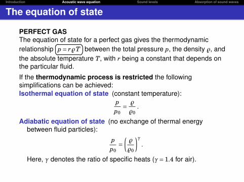
PERFECT GASThe equation of state for a perfect gas gives the thermodynamicrelationship
�� ��p= r%T between the total pressure p, the density %, andthe absolute temperature T, with r being a constant that depends onthe particular fluid.
If the thermodynamic process is restricted the followingsimplifications can be achieved:Isothermal equation of state (constant temperature):
pp0
= %
%0.
Adiabatic equation of state (no exchange of thermal energybetween fluid particles):
pp0
=(%
%0
)γ.
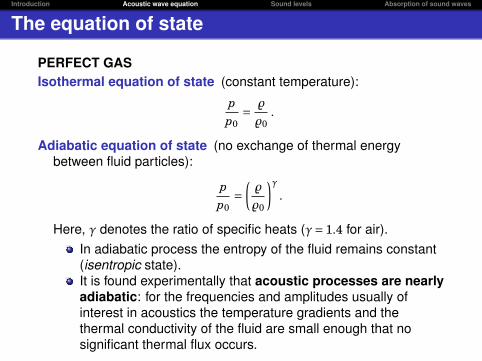
Here, γ denotes the ratio of specific heats (γ= 1.4 for air).In adiabatic process the entropy of the fluid remains constant(isentropic state).It is found experimentally that acoustic processes are nearlyadiabatic: for the frequencies and amplitudes usually ofinterest in acoustics the temperature gradients and thethermal conductivity of the fluid are small enough that nosignificant thermal flux occurs.
Introduction Acoustic wave equation Sound levels Absorption of sound waves
The equation of state
PERFECT GASThe equation of state for a perfect gas gives the thermodynamicrelationship
�� ��p= r%T between the total pressure p, the density %, andthe absolute temperature T, with r being a constant that depends onthe particular fluid.
If the thermodynamic process is restricted the followingsimplifications can be achieved:Isothermal equation of state (constant temperature):
pp0
= %
%0.
Adiabatic equation of state (no exchange of thermal energybetween fluid particles):
pp0
=(%
%0
)γ.
Here, γ denotes the ratio of specific heats (γ= 1.4 for air).
In adiabatic process the entropy of the fluid remains constant(isentropic state).It is found experimentally that acoustic processes are nearlyadiabatic: for the frequencies and amplitudes usually ofinterest in acoustics the temperature gradients and thethermal conductivity of the fluid are small enough that nosignificant thermal flux occurs.
Introduction Acoustic wave equation Sound levels Absorption of sound waves
The equation of state
PERFECT GASIsothermal equation of state (constant temperature):
pp0
= %
%0.
Adiabatic equation of state (no exchange of thermal energybetween fluid particles):
pp0
=(%
%0
)γ.
Here, γ denotes the ratio of specific heats (γ= 1.4 for air).In adiabatic process the entropy of the fluid remains constant(isentropic state).It is found experimentally that acoustic processes are nearlyadiabatic: for the frequencies and amplitudes usually ofinterest in acoustics the temperature gradients and thethermal conductivity of the fluid are small enough that nosignificant thermal flux occurs.

Introduction Acoustic wave equation Sound levels Absorption of sound waves
The equation of state
REAL FLUIDSThe adiabatic equation of state is more complicated.
It is then preferable to determine experimentally the isentropicrelationship between pressure and density fluctuations: p= p(%).A Taylor’s expansion can be written for this relationship:
p= p0 + ∂p∂%
∣∣∣∣%=%0
(%−%0)+ 12∂2p∂%2
∣∣∣∣%=%0
(%−%0)2 + . . .
where the partial derivatives are constants for the adiabaticcompression and expansion of the fluid about its equilibriumdensity %0.If the density fluctuations are small (i.e., %¿ %0) only the lowestorder term needs to be retained which gives a linear adiabaticequation of state:
p−p0 =K%−%0
%0→
�� ��p=K s
where K is the adiabatic bulk modulus. The essentialrestriction here is that the condensation must be small, i.e., s¿ 1.

Introduction Acoustic wave equation Sound levels Absorption of sound waves
The equation of state
REAL FLUIDSThe adiabatic equation of state is more complicated.It is then preferable to determine experimentally the isentropicrelationship between pressure and density fluctuations: p= p(%).
A Taylor’s expansion can be written for this relationship:
p= p0 + ∂p∂%
∣∣∣∣%=%0
(%−%0)+ 12∂2p∂%2
∣∣∣∣%=%0
(%−%0)2 + . . .
where the partial derivatives are constants for the adiabaticcompression and expansion of the fluid about its equilibriumdensity %0.If the density fluctuations are small (i.e., %¿ %0) only the lowestorder term needs to be retained which gives a linear adiabaticequation of state:
p−p0 =K%−%0
%0→
�� ��p=K s
where K is the adiabatic bulk modulus. The essentialrestriction here is that the condensation must be small, i.e., s¿ 1.

Introduction Acoustic wave equation Sound levels Absorption of sound waves
The equation of state
REAL FLUIDSThe adiabatic equation of state is more complicated.It is then preferable to determine experimentally the isentropicrelationship between pressure and density fluctuations: p= p(%).A Taylor’s expansion can be written for this relationship:
p= p0 + ∂p∂%
∣∣∣∣%=%0
(%−%0)+ 12∂2p∂%2
∣∣∣∣%=%0
(%−%0)2 + . . .
where the partial derivatives are constants for the adiabaticcompression and expansion of the fluid about its equilibriumdensity %0.
If the density fluctuations are small (i.e., %¿ %0) only the lowestorder term needs to be retained which gives a linear adiabaticequation of state:
p−p0 =K%−%0
%0→
�� ��p=K s
where K is the adiabatic bulk modulus. The essentialrestriction here is that the condensation must be small, i.e., s¿ 1.

Introduction Acoustic wave equation Sound levels Absorption of sound waves
The equation of state
REAL FLUIDSThe adiabatic equation of state is more complicated.It is then preferable to determine experimentally the isentropicrelationship between pressure and density fluctuations: p= p(%).A Taylor’s expansion can be written for this relationship:
p= p0 + ∂p∂%
∣∣∣∣%=%0
(%−%0)+ 12∂2p∂%2
∣∣∣∣%=%0
(%−%0)2 + . . .
where the partial derivatives are constants for the adiabaticcompression and expansion of the fluid about its equilibriumdensity %0.If the density fluctuations are small (i.e., %¿ %0) only the lowestorder term needs to be retained which gives a linear adiabaticequation of state:
p−p0 =K%−%0
%0→
�� ��p=K s
where K is the adiabatic bulk modulus. The essentialrestriction here is that the condensation must be small, i.e., s¿ 1.

Introduction Acoustic wave equation Sound levels Absorption of sound waves
Continuity equation
The continuity equation describes the conservative transport ofmass. (Similar continuity equations are also derived for otherquantities which are conserved, like energy, momentum, etc.)
It may be derived by considering the fluxes into an infinitesimalbox of volume dV = dx dy dz.
The net flux for the x direction:%u1 −
(%u1 +
∂%u1∂x
dx)dydz=− ∂%u1
∂xdV
The total influx is the sum of the fluxes in all directions:−
(∂%u1∂x
+ ∂%u2∂y
+ ∂%u3∂z
)dV =−∇· (%u) dV
The rate with which the mass increase in the volume:∂%
∂tdV
The continuity equation results from the fact that the rate ofincrease must be equal to the net influx.
Continuity equation:
∂%
∂t+∇·(%u)= 0 linearization−−−−−−−−−→
%(x,t)=%0+%(x,t)%, u – small
�
�∂%
∂t+%0∇·u= 0 −−−−→
%=%0 s
∂s∂t
+∇·u= 0
The continuity equation is integrated with respect to time∫ (∂s∂t
+∇·u)dt= s+∇·ξ= (constant=)0 → s=−∇·ξ
where the integration constant must be zero since there is nodisturbance, and
∫ ∇·udt=∇·∫ udt=∇·∫ ∂ξ∂t dt=∇·ξ.
The result is combined with the adiabatic equation of statep=K s, which shows that the pressure in fluid depends on thevolume dilatation trε=∇·ξ:
p=−K∇·ξ=−K trε

Introduction Acoustic wave equation Sound levels Absorption of sound waves
Continuity equation
The continuity equation describes the conservative transport ofmass. (Similar continuity equations are also derived for otherquantities which are conserved, like energy, momentum, etc.)It may be derived by considering the fluxes into an infinitesimalbox of volume dV = dx dy dz.
The net flux for the x direction:%u1 −
(%u1 +
∂%u1∂x
dx)dydz=− ∂%u1
∂xdV
The total influx is the sum of the fluxes in all directions:−
(∂%u1∂x
+ ∂%u2∂y
+ ∂%u3∂z
)dV =−∇· (%u) dV
The rate with which the mass increase in the volume:∂%
∂tdV
The continuity equation results from the fact that the rate ofincrease must be equal to the net influx.
Continuity equation:
∂%
∂t+∇·(%u)= 0 linearization−−−−−−−−−→
%(x,t)=%0+%(x,t)%, u – small
�
�∂%
∂t+%0∇·u= 0 −−−−→
%=%0 s
∂s∂t
+∇·u= 0
The continuity equation is integrated with respect to time∫ (∂s∂t
+∇·u)dt= s+∇·ξ= (constant=)0 → s=−∇·ξ
where the integration constant must be zero since there is nodisturbance, and
∫ ∇·udt=∇·∫ udt=∇·∫ ∂ξ∂t dt=∇·ξ.
The result is combined with the adiabatic equation of statep=K s, which shows that the pressure in fluid depends on thevolume dilatation trε=∇·ξ:
p=−K∇·ξ=−K trε

Introduction Acoustic wave equation Sound levels Absorption of sound waves
Continuity equation
Continuity equation:
∂%
∂t+∇·(%u)= 0 linearization−−−−−−−−−→
%(x,t)=%0+%(x,t)%, u – small
�
�∂%
∂t+%0∇·u= 0 −−−−→
%=%0 s
∂s∂t
+∇·u= 0
The continuity equation is integrated with respect to time∫ (∂s∂t
+∇·u)dt= s+∇·ξ= (constant=)0 → s=−∇·ξ
where the integration constant must be zero since there is nodisturbance, and
∫ ∇·udt=∇·∫ udt=∇·∫ ∂ξ∂t dt=∇·ξ.
The result is combined with the adiabatic equation of statep=K s, which shows that the pressure in fluid depends on thevolume dilatation trε=∇·ξ:
p=−K∇·ξ=−K trε

Introduction Acoustic wave equation Sound levels Absorption of sound waves
Equilibrium equation
Consider a fluid element dV which moves with the fluid. Themass of the element equals dm= % dV.In the absence of viscosity, the net force experienced by theelement is: df =−∇p dV.The acceleration of the fluid element (following the fluid) is thesum of the rate of change of velocity in the fixed position in space
and the convective part: a= ∂u∂t
+ (u ·∇)u.
According to Newton’s second law:�� ��dma= df
Momentum equation (Euler’s equation):
%
(∂u∂t
+u ·∇u)=−∇p linearization−−−−−−−−−→
%(x,t)=%0+%(x,t)%, u – small
�
�%0
∂u∂t
=−∇p
This linear, inviscid momentum equation is valid for acousticprocesses of small amplitude.

Introduction Acoustic wave equation Sound levels Absorption of sound waves
Linear wave equation
The linearized continuity equation:∂%
∂t+%0∇·u= 0
is time-differentiated.
The linearized momentum equation: %0∂u∂t
=−∇p
is subject to divergence operation.Now, their combination yields:
∂2%
∂t2 −4p= 0
The equation of state relates the pressure withdensity-fluctuation:
p= p(%) → 4p= ∂p∂%
4%+ ∂2p∂%2 (∇%)2 = ∂p
∂%4%
Wave equation for the density-fluctuation field�
�∂2%
∂t2 −c204%= 0 where c0 =
√∂p∂%
is the acoustic wave velocity (or the speed of sound).

Introduction Acoustic wave equation Sound levels Absorption of sound waves
Linear wave equation
The linearized continuity equation:∂%
∂t+%0∇·u= 0
is time-differentiated.The linearized momentum equation: %0
∂u∂t
=−∇p
is subject to divergence operation.Now, their combination yields:
∂2%
∂t2 −4p= 0
The equation of state relates the pressure withdensity-fluctuation:
p= p(%) → 4p= ∂p∂%
4%+ ∂2p∂%2 (∇%)2 = ∂p
∂%4%
For elastic fluids: p= p0 +K%
%0and then
∂p∂%
= K%0
.
Wave equation for the density-fluctuation field�
�∂2%
∂t2 −c204%= 0 where c0 =
√∂p∂%
is the acoustic wave velocity (or the speed of sound).

Introduction Acoustic wave equation Sound levels Absorption of sound waves
Linear wave equation
The linearized continuity equation:∂%
∂t+%0∇·u= 0
is time-differentiated.The linearized momentum equation: %0
∂u∂t
=−∇p
is subject to divergence operation.Now, their combination yields:
∂2%
∂t2 −4p= 0
The equation of state relates the pressure withdensity-fluctuation:
p= p(%) → 4p= ∂p∂%
4%+ ∂2p∂%2 (∇%)2 = ∂p
∂%4%
Wave equation for the density-fluctuation field�
�∂2%
∂t2 −c204%= 0 where c0 =
√∂p∂%
is the acoustic wave velocity (or the speed of sound).

Introduction Acoustic wave equation Sound levels Absorption of sound waves
Linear wave equationNotice that:
%(x, t)= %0 + %(x,t),p and % are proportional,p(x, t)= p0 + p(x, t),%(x, t)= %0 s(x,t).
Therefore, the wave equation is satisfied by:the instantaneous pressure: ∂2p
∂t2 = c204p
the acoustic pressure:�
�∂2p
∂t2 = c204p
the instantaneous density: ∂2%
∂t2 = c204%
the density-fluctuation: ∂2%
∂t2 = c204%
the condensation: ∂2 s∂t2 = c2
04s
Velocity potentialBy applying the curl to the linearized momentum equation one showsthat the particle velocity field is irrotational, ∇×u= 0. Therefore, itcan be expressed as the gradient of a scalar function φ(x, t) known asthe velocity potential:
�� ��u=∇φ .
the velocity potential: ∂2φ
∂t2 = c204φ
the particle velocity: ∂2u∂t2 = c2
04u

Introduction Acoustic wave equation Sound levels Absorption of sound waves
Linear wave equationThe wave equation is satisfied by:
the instantaneous pressure: ∂2p∂t2 = c2
04p
the acoustic pressure:�
�∂2p
∂t2 = c204p
the instantaneous density: ∂2%
∂t2 = c204%
the density-fluctuation: ∂2%
∂t2 = c204%
the condensation: ∂2 s∂t2 = c2
04s
Velocity potentialBy applying the curl to the linearized momentum equation one showsthat the particle velocity field is irrotational, ∇×u= 0. Therefore, itcan be expressed as the gradient of a scalar function φ(x, t) known asthe velocity potential:
�� ��u=∇φ .
the velocity potential: ∂2φ
∂t2 = c204φ
the particle velocity: ∂2u∂t2 = c2
04u

Introduction Acoustic wave equation Sound levels Absorption of sound waves
The speed of sound
Inviscid isotropic elastic liquid. The pressure in an inviscid liquiddepends on the volume dilatation trε: p=−K trε , where K is thebulk modulus. Now,
p=K sp=p−p0−−−−−→
s= %%0
p= p0+ K%0
% → c20 =
∂p∂%
= K%0
→��
� c0 =
√K%0
Perfect gas. The determination of speed of sound in a perfect gas iscomplicated and requires the use of thermodynamicconsiderations. The final result is
c0 =√γ
p0
%0=
√γRT0 ,
where γ denotes the ratio of specific heats (γ= 1.4 for air), R is theuniversal gas constant, and T0 is the (isothermal) temperature.For air at 20◦C and normal atmospheric pressure: c0 = 340 m
s .

Introduction Acoustic wave equation Sound levels Absorption of sound waves
Inhomogeneous wave equation
The wave equation has been developed for regions of space notcontaining any sources of acoustic energy.However, a source must be present to generate any acousticdisturbance. If the source is external to the region of interest, itcan be realized by time-dependent boundary conditions.Alternately, the acoustic equations can be modified to includesource terms.
Main types of acoustic energy sources:Monopole source: a closed surface that changes volume (e.g., a
loudspeaker in an enclosed cabinet) – a mass is being injectedinto the space at a rate per unit volume G(x,t), and the linearized
continuity equation becomes:∂%
∂t+%0∇·u=G .
Dipole source: a body oscillating back and forth without anychange in volume (e.g., the cone of an unbaffled loudspeaker) –there are body forces (per unit volume) f (x, t) present in the fluid,
and the linearized momentum equation becomes: %0∂u∂t
+∇p= f .
Taking into account internal sources introduces an inhomogeneousterm into the wave equation.
Inhomogeneous wave equation
∂2%
∂t2 −c204%=
∂G∂t
−∇· f or1c2
0
∂2p∂t2 −4p= ∂G
∂t−∇· f etc.

Introduction Acoustic wave equation Sound levels Absorption of sound waves
Inhomogeneous wave equation
Main types of acoustic energy sources:Monopole source: a closed surface that changes volume (e.g., a
loudspeaker in an enclosed cabinet) – a mass is being injectedinto the space at a rate per unit volume G(x,t), and the linearized
continuity equation becomes:∂%
∂t+%0∇·u=G .
Dipole source: a body oscillating back and forth without anychange in volume (e.g., the cone of an unbaffled loudspeaker) –there are body forces (per unit volume) f (x, t) present in the fluid,
and the linearized momentum equation becomes: %0∂u∂t
+∇p= f .
Taking into account internal sources introduces an inhomogeneousterm into the wave equation.
Inhomogeneous wave equation
∂2%
∂t2 −c204%=
∂G∂t
−∇· f or1c2
0
∂2p∂t2 −4p= ∂G
∂t−∇· f etc.

Introduction Acoustic wave equation Sound levels Absorption of sound waves
Acoustic impedanceA general concept of impedance
Impedance can be generally described as the ratio of a “push”variable (such as voltage or pressure) to a corresponding “flow”variable (such as current or particle velocity).
Definition (Mechanical impedance = force/velocity)
Mechanical impedance of a point on a structure is the ratio of theforce applied to the point to the resulting velocity at that point.
Definition (Acoustic impedance = pressure/velocity)
Specific acoustic impedance:�� ��Z= p
u (u≡ |u|).It is the ratio of the acoustic pressure in a medium to theassociated particle speed.
Definition (Characteristic acoustic impedance)
Characteristic impedance of a medium:�� ��Z0 = %0 c0 .
For traveling plane waves pressure and particle velocity are related toeach other as follows:
forward traveling waves: p=Z0 u,backward traveling waves: p=−Z0 u.
%0 c0 Z0 = %0 c0Medium
[kgm3
] [ms
] [Pa·sm
]Air 1.21 343 415Distilled water 998 1482 1.48×10⁶
Thin aluminium rod 2700 5050 1.36×10⁷

Introduction Acoustic wave equation Sound levels Absorption of sound waves
Acoustic impedanceA general concept of impedance
Impedance can be generally described as the ratio of a “push”variable (such as voltage or pressure) to a corresponding “flow”variable (such as current or particle velocity).
Impedance is a frequency-domain concept: for linear systems,if the “push” is a time-harmonic function the related “flow” mustalso be time harmonic, and then the time dependance cancelswhich makes the impedance ratio a very useful quantity – ingeneral frequency-dependent.The “push” and “flow” variables are in general complex, so is theimpedance.In certain instances, however, it is not necessary to assumetime-harmonic signals because the time dependance cancelsregardless of the waveform. The impedance in these cases isreal and frequency-independent. (Example: plane soundwaves in lossless fluids.)
Definition (Mechanical impedance = force/velocity)
Mechanical impedance of a point on a structure is the ratio of theforce applied to the point to the resulting velocity at that point.
Definition (Acoustic impedance = pressure/velocity)
Specific acoustic impedance:�� ��Z= p
u (u≡ |u|).It is the ratio of the acoustic pressure in a medium to theassociated particle speed.
Definition (Characteristic acoustic impedance)
Characteristic impedance of a medium:�� ��Z0 = %0 c0 .
For traveling plane waves pressure and particle velocity are related toeach other as follows:
forward traveling waves: p=Z0 u,backward traveling waves: p=−Z0 u.
%0 c0 Z0 = %0 c0Medium
[kgm3
] [ms
] [Pa·sm
]Air 1.21 343 415Distilled water 998 1482 1.48×10⁶
Thin aluminium rod 2700 5050 1.36×10⁷

Introduction Acoustic wave equation Sound levels Absorption of sound waves
Acoustic impedanceA general concept of impedance
Impedance can be generally described as the ratio of a “push”variable (such as voltage or pressure) to a corresponding “flow”variable (such as current or particle velocity).
Definition (Mechanical impedance = force/velocity)
Mechanical impedance of a point on a structure is the ratio of theforce applied to the point to the resulting velocity at that point. It isthe inverse of mechanical admittance or mobility, and a measureof how much a structure resists motion when subjected to a givenforce. Usefulness: coupling between acoustic waves and a drivingsource or driven load.
Definition (Acoustic impedance = pressure/velocity)
Specific acoustic impedance:�� ��Z= p
u (u≡ |u|).It is the ratio of the acoustic pressure in a medium to theassociated particle speed.
Definition (Characteristic acoustic impedance)
Characteristic impedance of a medium:�� ��Z0 = %0 c0 .
For traveling plane waves pressure and particle velocity are related toeach other as follows:
forward traveling waves: p=Z0 u,backward traveling waves: p=−Z0 u.
%0 c0 Z0 = %0 c0Medium
[kgm3
] [ms
] [Pa·sm
]Air 1.21 343 415Distilled water 998 1482 1.48×10⁶
Thin aluminium rod 2700 5050 1.36×10⁷

Introduction Acoustic wave equation Sound levels Absorption of sound waves
Acoustic impedanceA general concept of impedance
Impedance can be generally described as the ratio of a “push”variable (such as voltage or pressure) to a corresponding “flow”variable (such as current or particle velocity).
Definition (Mechanical impedance = force/velocity)
Mechanical impedance of a point on a structure is the ratio of theforce applied to the point to the resulting velocity at that point.
Definition (Acoustic impedance = pressure/velocity)
Specific acoustic impedance:�� ��Z= p
u (u≡ |u|).It is the ratio of the acoustic pressure in a medium to theassociated particle speed. Usefulness: transmission ofacoustic waves from one medium to another.Acoustic impedance at a given surface is the ratio of the acousticpressure averaged over that surface to the volume velocity through thesurface. Usefulness: radiation from vibrating surfaces.
Definition (Characteristic acoustic impedance)
Characteristic impedance of a medium:�� ��Z0 = %0 c0 .
For traveling plane waves pressure and particle velocity are related toeach other as follows:
forward traveling waves: p=Z0 u,backward traveling waves: p=−Z0 u.
%0 c0 Z0 = %0 c0Medium
[kgm3
] [ms
] [Pa·sm
]Air 1.21 343 415Distilled water 998 1482 1.48×10⁶
Thin aluminium rod 2700 5050 1.36×10⁷

Introduction Acoustic wave equation Sound levels Absorption of sound waves
Acoustic impedanceDefinition (Acoustic impedance = pressure/velocity)
Specific acoustic impedance:�� ��Z= p
u (u≡ |u|).It is the ratio of the acoustic pressure in a medium to theassociated particle speed.
Definition (Characteristic acoustic impedance)
Characteristic impedance of a medium:�� ��Z0 = %0 c0 .
For traveling plane waves pressure and particle velocity are related toeach other as follows:
forward traveling waves: p=Z0 u,backward traveling waves: p=−Z0 u.
%0 c0 Z0 = %0 c0Medium
[kgm3
] [ms
] [Pa·sm
]Air 1.21 343 415Distilled water 998 1482 1.48×10⁶
Thin aluminium rod 2700 5050 1.36×10⁷

Introduction Acoustic wave equation Sound levels Absorption of sound waves
Acoustic boundary conditionsThe acoustic wave equation (written here for the acousticpressure p, with monopole source g= ∂G
∂t , and dipole source f )
1c2
0
∂2p∂t2 −∇· (
−%0∂u∂t︷ ︸︸ ︷
∇p− f)= g
is an example of hyperbolic PDE.
Boundary conditions:1 (Dirichlet b.c.) Imposed pressure ˆp:
p= ˆp
For ˆp= 0: the sound soft boundary.2 (Neumann b.c.) Imposed normal acceleration an:
∂u∂t
·n=− 1%0
(∇p− f) ·n= an
For an = 0: the sound hard boundary (rigid wall).3 (Robin b.c.) Specified impedance Z:
− 1%0
(∇p− f) ·n+ 1
Z∂p∂t
= an (usually an = 0)
For Z=Z0 = %0 c0 (and an = 0): non reflection condition (the planewave radiates into infinity).

Introduction Acoustic wave equation Sound levels Absorption of sound waves
Acoustic boundary conditions
1c2
0
∂2p∂t2 −∇· (
−%0∂u∂t︷ ︸︸ ︷
∇p− f)= g
Boundary conditions:1 (Dirichlet b.c.) Imposed pressure ˆp:
p= ˆp
For ˆp= 0: the sound soft boundary.2 (Neumann b.c.) Imposed normal acceleration an:
∂u∂t
·n=− 1%0
(∇p− f) ·n= an
For an = 0: the sound hard boundary (rigid wall).3 (Robin b.c.) Specified impedance Z:
− 1%0
(∇p− f) ·n+ 1
Z∂p∂t
= an (usually an = 0)
For Z=Z0 = %0 c0 (and an = 0): non reflection condition (the planewave radiates into infinity).

Introduction Acoustic wave equation Sound levels Absorption of sound waves
Outline
1 IntroductionSound wavesAcoustic variables
2 Acoustic wave equationAssumptionsThe equation of stateContinuity equationEquilibrium equationLinear wave equationThe speed of soundInhomogeneous waveequationAcoustic impedanceAcoustic boundaryconditions
3 Sound levelsSound intensity and powerDecibel scalesSound pressure levelEqual-loudness contours
4 Absorption of sound wavesMechanisms of theacoustic energy dissipationA phenomenologicalapproach to absorptionThe classical absorptioncoefficient

Introduction Acoustic wave equation Sound levels Absorption of sound waves
Sound intensity and powerThe propagation of acoustic wave is accompanied by a flow of energyin the direction the wave is traveling.
Definition (Sound intensity)
Sound intensity I in a specified direction n is defined as the timeaverage of energy flow (i.e., power) through a unit area ∆A(perpendicular to the specified direction).
power= force ·velocity= p∆An ·u → power∆A
= pu ·n
I = I ·n= 1tav
tav∫0
pu ·ndt and I = 1tav
tav∫0
pudt
where u ·n= |u| ≡ u if n is identical with the direction of propagation,whereas tav is the averaging time (it depends on the waveform type):
for periodic waves tav is the period,
for transient signals tav is their duration,
for nonperiodic waves tav →∞.
Definition (Sound power)
Sound power W passing through a surface S is the integral of theintensity over the surface:
W =∫S
I ·dS

Introduction Acoustic wave equation Sound levels Absorption of sound waves
Sound intensity and power
Definition (Sound intensity)
I = I ·n= 1tav
tav∫0
pu ·ndt and I = 1tav
tav∫0
pudt
where u ·n= |u| ≡ u if n is identical with the direction of propagation,whereas tav is the averaging time.
Progressive waves of arbitrary waveform in lossless fluids:Forward traveling waves: u= p
Z0and then
I = 1tav
tav∫0
p2
Z0dt= p2
rmsZ0
where
��
��prms =
√√√√√ 1tav
tav∫0
p2 dt
is the root-mean-square pressure (for example, if p is asinusoidal signal of amplitude A: prms = Ap
2).
Backward traveling waves: u=− pZ0
and I =− p2rmsZ0
which isnegative because the energy travels in the opposite direction.
Definition (Sound power)
Sound power W passing through a surface S is the integral of theintensity over the surface:
W =∫S
I ·dS

Introduction Acoustic wave equation Sound levels Absorption of sound waves
Sound intensity and power
Definition (Sound intensity)
I = I ·n= 1tav
tav∫0
pu ·ndt and I = 1tav
tav∫0
pudt
where u ·n= |u| ≡ u if n is identical with the direction of propagation,whereas tav is the averaging time.
Definition (Sound power)
Sound power W passing through a surface S is the integral of theintensity over the surface:
W =∫S
I ·dS

Introduction Acoustic wave equation Sound levels Absorption of sound waves
Decibel scalesSound pressures, intensities and powers are customarily describedby logarithmic scales known as sound levels:
SPL – sound pressure level,SIL – sound intensity level,
SWL – sound power level.
Sound pressure level (SPL)
Lp = 20log10
(prms
pref
) [dB
]
Sound intensity level (SIL)
LI = 10log10
(I
Iref
) [dB
]
Sound power level (SWL)
LW = 10log10
(W
Wref
) [dB
]where Wref is a reference. SWL is a measure of the total acousticenergy per unit time emitted by a source.

Introduction Acoustic wave equation Sound levels Absorption of sound waves
Decibel scalesSound pressures, intensities and powers are customarily describedby logarithmic scales known as sound levels:
SPL – sound pressure level,SIL – sound intensity level,
SWL – sound power level.There are two reasons for doing this:
1 A wide range of sound pressures and intensities areencountered in the acoustic environment, for example:
audible acoustic pressure range from 10−5 to more than 100 Pa,audible intensities range from approximately 10−12 to 10 W
m2 .The use of logarithmic scale compresses the range of numbersrequired to describe such wide ranges.
2 The relative loudness of two sounds is judged by human ear bythe ratio of their intensities (which is a logarithmic behaviour).
Sound pressure level (SPL)
Lp = 20log10
(prms
pref
) [dB
]
Sound intensity level (SIL)
LI = 10log10
(I
Iref
) [dB
]
Sound power level (SWL)
LW = 10log10
(W
Wref
) [dB
]where Wref is a reference. SWL is a measure of the total acousticenergy per unit time emitted by a source.

Introduction Acoustic wave equation Sound levels Absorption of sound waves
Decibel scalesSound pressures, intensities and powers are customarily describedby logarithmic scales known as sound levels:
Sound pressure level (SPL)
Lp = 10log10
(p2
rms
p2ref
)= 20log10
(prms
pref
) [dB
]where pref is a reference pressure.
For air: pref = 2×10⁻⁵ Pa= 20µPaFor water: pref = 10−6 Pa= 1µPa
Sound intensity level (SIL)
LI = 10log10
(I
Iref
) [dB
]
Sound power level (SWL)
LW = 10log10
(W
Wref
) [dB
]where Wref is a reference. SWL is a measure of the total acousticenergy per unit time emitted by a source.

Introduction Acoustic wave equation Sound levels Absorption of sound waves
Decibel scalesSound pressures, intensities and powers are customarily describedby logarithmic scales known as sound levels:
Sound pressure level (SPL)
Lp = 20log10
(prms
pref
) [dB
](for air: pref = 20µPa)
Sound intensity level (SIL)
LI = 10log10
(I
Iref
) [dB
]where Iref is a reference intensity. The standard reference intensity forairborne sounds is Iref = 10−12 W
m2 . (This is approximately the intensityof barely-audible pure tone of 1 kHz.)
Sound power level (SWL)
LW = 10log10
(W
Wref
) [dB
]where Wref is a reference. SWL is a measure of the total acousticenergy per unit time emitted by a source.

Introduction Acoustic wave equation Sound levels Absorption of sound waves
Decibel scalesSound pressures, intensities and powers are customarily describedby logarithmic scales known as sound levels:
Sound pressure level (SPL)
Lp = 20log10
(prms
pref
) [dB
](for air: pref = 20µPa)
Sound intensity level (SIL)
LI = 10log10
(I
Iref
) [dB
](for air: Iref = 10−12 W
m2 )
For traveling and spherical waves I = p2rms%0 c0
. Therefore, for progressivewaves in air SPL and SIL are (in practice) numerically the same since:
LI = 10log10
(p2
rms%0 c0 Iref
p2ref
p2ref
)= 20log10
(prms
pref
)︸ ︷︷ ︸
Lp
+10log10
( p2ref
%0 c0 Iref
)︸ ︷︷ ︸
−0.16dB
∼=Lp
Sound power level (SWL)
LW = 10log10
(W
Wref
) [dB
]where Wref is a reference. SWL is a measure of the total acousticenergy per unit time emitted by a source.

Introduction Acoustic wave equation Sound levels Absorption of sound waves
Decibel scalesSound pressures, intensities and powers are customarily describedby logarithmic scales known as sound levels:
Sound pressure level (SPL)
Lp = 20log10
(prms
pref
) [dB
](for air: pref = 20µPa)
Sound intensity level (SIL)
LI = 10log10
(I
Iref
) [dB
](for air: Iref = 10−12 W
m2 )
Sound power level (SWL)
LW = 10log10
(W
Wref
) [dB
](for air: Wref = 10−12 W)
where Wref is a reference. SWL is a measure of the total acousticenergy per unit time emitted by a source.

Introduction Acoustic wave equation Sound levels Absorption of sound waves
Sound pressure level
prms SPLSource (or character) of sound [Pa] [dB]threshold of pain 100 134hearing damage during short-term effect 20 ∼120jet engine, 100 m distant 6–200 110–140hammer drill, 1 m distant 2 ∼100hearing damage from long-term exposure 0.6 ∼85traffic noise on major road, 10 m distant 0.2–0.6 80–90moving automobile, 10 m distant 0.02–0.2 60–80TV set (typical loudness), 1 m distant 0.02 ∼60normal talking, 1 m distant 0.002–0.02 40–60very calm room 0.0002–0.0006 20–30calm human breathing 0.00006 10auditory threshold at 2 kHz 0.00002 0
(dB re 20µPa)

Introduction Acoustic wave equation Sound levels Absorption of sound waves
Equal-loudness contours

Introduction Acoustic wave equation Sound levels Absorption of sound waves
Outline
1 IntroductionSound wavesAcoustic variables
2 Acoustic wave equationAssumptionsThe equation of stateContinuity equationEquilibrium equationLinear wave equationThe speed of soundInhomogeneous waveequationAcoustic impedanceAcoustic boundaryconditions
3 Sound levelsSound intensity and powerDecibel scalesSound pressure levelEqual-loudness contours
4 Absorption of sound wavesMechanisms of theacoustic energy dissipationA phenomenologicalapproach to absorptionThe classical absorptioncoefficient

Introduction Acoustic wave equation Sound levels Absorption of sound waves
Mechanisms of the acoustic energy dissipation
All acoustic energy is dissipated into thermal energy.Dissipation is often very slow and it can be ignored for smalldistances or short times.
Sources of dissipation are due to:1 losses at the boundaries (relevant for porous materials, thin
ducts, and small rooms);2 losses in the medium (important when the volume of fluid is
large).
Relaxation timeEach absorption process is characterized by its relaxation time, thatis, the amount of time for the particular process to be nearlycompleted.

Introduction Acoustic wave equation Sound levels Absorption of sound waves
Mechanisms of the acoustic energy dissipation
All acoustic energy is dissipated into thermal energy.Dissipation is often very slow and it can be ignored for smalldistances or short times.
Sources of dissipation are due to:1 losses at the boundaries (relevant for porous materials, thin
ducts, and small rooms);2 losses in the medium (important when the volume of fluid is
large). Here, the losses are associated with:viscosity – frictional losses resulting from the relative motionbetween adjacent portions of the medium (during its compressionsand expansions);
heat conductionmolecular exchanges of energy
Relaxation timeEach absorption process is characterized by its relaxation time, thatis, the amount of time for the particular process to be nearlycompleted.

Introduction Acoustic wave equation Sound levels Absorption of sound waves
Mechanisms of the acoustic energy dissipation
All acoustic energy is dissipated into thermal energy.Dissipation is often very slow and it can be ignored for smalldistances or short times.
Sources of dissipation are due to:1 losses at the boundaries (relevant for porous materials, thin
ducts, and small rooms);2 losses in the medium (important when the volume of fluid is
large). Here, the losses are associated with:viscosityheat conduction – losses resulting from the conduction of thermalenergy between higher temperature condensations and lowertemperature rarefactions;
molecular exchanges of energy
Relaxation timeEach absorption process is characterized by its relaxation time, thatis, the amount of time for the particular process to be nearlycompleted.

Introduction Acoustic wave equation Sound levels Absorption of sound waves
Mechanisms of the acoustic energy dissipation
All acoustic energy is dissipated into thermal energy.Dissipation is often very slow and it can be ignored for smalldistances or short times.
Sources of dissipation are due to:1 losses at the boundaries (relevant for porous materials, thin
ducts, and small rooms);2 losses in the medium (important when the volume of fluid is
large). Here, the losses are associated with:viscosityheat conductionmolecular exchanges of energy – the conversion of kineticenergy of molecules into: stored potential energy (structuralrearrangement of adjacent molecules), or internal rotational andvibrational energies (for polyatomic molecules), or energies ofassociation and dissociation between different ionic species.
Relaxation timeEach absorption process is characterized by its relaxation time, thatis, the amount of time for the particular process to be nearlycompleted.

Introduction Acoustic wave equation Sound levels Absorption of sound waves
Mechanisms of the acoustic energy dissipation
All acoustic energy is dissipated into thermal energy.Dissipation is often very slow and it can be ignored for smalldistances or short times.
Sources of dissipation are due to:1 losses at the boundaries (relevant for porous materials, thin
ducts, and small rooms);2 losses in the medium (important when the volume of fluid is
large). Here, the losses are associated with:viscosityheat conductionmolecular exchanges of energy
Relaxation timeEach absorption process is characterized by its relaxation time, thatis, the amount of time for the particular process to be nearlycompleted.

Introduction Acoustic wave equation Sound levels Absorption of sound waves
A phenomenological approach to absorption
No acoustic energy loss. A consequence of ignoring any lossmechanisms is that the acoustic pressure p and condensation s arein phase as related by the linear equation of state:
p= %0 c20 s
Energy loss. One way to introduce losses is to allow a delaybetween the application of a sudden pressure change p0 and theattainment of the resulting equilibrium condensation seq, which canbe yielded by a modified equation of state (Stokes):
p= %0 c20
(1+τ ∂
∂t
)s
where τ is the relaxation time.
Lossy acoustic-wave equation
1c2
0
∂2p∂t2 −
(1+τ ∂
∂t
)4p= 0
Lossy Helmholtz equation(4+k2)p= 0 where k= ω
c0
1p1+ iωτ

Introduction Acoustic wave equation Sound levels Absorption of sound waves
A phenomenological approach to absorptionEnergy loss. One way to introduce losses is to allow a delay
between the application of a sudden pressure change p0 and theattainment of the resulting equilibrium condensation seq, which canbe yielded by a modified equation of state (Stokes):
p= %0 c20
(1+τ ∂
∂t
)s
where τ is the relaxation time: at t= τ the condensation reaches1− 1
e = 0.632 of its final equilibrium value seq = p0%0 c2
0.
Response of a relaxing fluid to a sudden increase in pressures
t
lossy responses= seq
(1−exp(−t/τ)
)seq
no-loss response
(1− 1
e)seq = 0.632 seq
τ0
Lossy acoustic-wave equation
1c2
0
∂2p∂t2 −
(1+τ ∂
∂t
)4p= 0
Lossy Helmholtz equation(4+k2)p= 0 where k= ω
c0
1p1+ iωτ

Introduction Acoustic wave equation Sound levels Absorption of sound waves
A phenomenological approach to absorption
Energy loss. One way to introduce losses is to allow a delaybetween the application of a sudden pressure change p0 and theattainment of the resulting equilibrium condensation seq, which canbe yielded by a modified equation of state (Stokes):
p= %0 c20
(1+τ ∂
∂t
)s
where τ is the relaxation time: at t= τ the condensation reaches1− 1
e = 0.632 of its final equilibrium value seq = p0%0 c2
0.
Lossy acoustic-wave equation
1c2
0
∂2p∂t2 −
(1+τ ∂
∂t
)4p= 0
Lossy Helmholtz equation(4+k2)p= 0 where k= ω
c0
1p1+ iωτ

Introduction Acoustic wave equation Sound levels Absorption of sound waves
The classical absorption coefficientRelaxation times and absorption coefficients associated with:
viscous losses (µ is the viscosity):
τµ = 43
µ
%0 c20
→ αµ ≈ 23
ω2
%0 c30µ
thermal conduction losses (κ is the thermal conduction):
τκ = 1%0 c2
0
κ
Cp→ ακ ≈ 1
2ω2
%0 c30
γ−1Cp
κ
(In gases: τµ,τκ ∼ 10−10 s; in liquids: τµ,τκ ∼ 10−12 s.)
Classical absorption coefficient
α≈αµ+ακ ≈ ω2
2%0 c30
[43µ+ γ−1
Cpκ
]= ω2µ
2%0 c30
[43+ γ−1
Pr
]where Pr= µC
κis the Prandtl number which measures the
importance of the effects of viscosity relative to the effects of thermalconduction.