1

1. Use the IS-LM model to determine the effects of each of the following on thegeneral equilibrium values of the real wage, employment, output, the real interest rate,consumption, investment, and the price level.

a. A reduction in the effective tax rate on capital that increases desired investment.

Answer:

Id r; MPK f , τ( )If ↓τ, then the investment schedule shifts to the right.

Adjustment story: at ro the level of desired savings is less than the level of desiredinvestment. That is equivalent to saying the following

Y < Cd+Id+Gi.e., the Goods Market is not in equilibrium at ro. Explain adjustment in the goodsmarket in terms of movements along desired savings and desired investment. (Notethat we are assuming that prices of the goods are not changing)

at ro : Y < cd + Id + G

⇒ consumers save less and firms invest more when the interst rate it low

2

⇒ ↑ r eliminates the excess demand for goods over the supply by ↓cd & ↓Id until Y = cd + Id + G

adjustment along the savings schedule:

↑r ⇒ ↑Sd = Y− ↓Cd −G

adjustment along the investment schedule:

↑r ⇒ ↑r + d( )pk = ↑uc

⇒↓It = ↓K∗ − Kt + dKt

Now we can write out the IS function explicitly

IS r, Y; yfe , W, G, T, MPKf , τ

If ↓τ then the IS curve shifts up, i.e., to the right.

Note that when we consider changes in r and Y, then we are contemplatingmovements along the IS curve!

When an exogenous variable changes, we are considering what happens to theequilibrium interest rate for a given level of output, Y.

Asset Market Equilibrium:

Recall our money demand function

Md = PL Y, r + πe( )In equilibrium

Ms = Md

⇒ Ms = PL Y, r + πe( )⇒ M

s

P = L Y, r + πe( )

3

Now we can graph this relationship

Money supply changes: ↑P shifts the money supply curve to the left

Adjustment Story: at r1 the quantity of money demanded exceeds the quantity ofmoney supplied. As money holders sell some of their nonmonetary assets so they canhold more money in their portfolios, the price of nonmonetary assets is driven down.This raises the real interest rate on nonmonetary assets. As r rises the quantity ofmoney demanded falls (movement along a negatively sloped money demand curve),until equilibrium is reached. Show with the money demand equation.

4

5

b. The expected rate of inflation rises.

Answer: If ↑πethen real money demand falls, i.e., shifts back.

Adjustment Story: at the old interest rate, the supply of money exceeds thequantity of money demanded. Agents purchase nonmonetary assets, driving theirprices up and their real returns (the real interest rate paid on the asset) down. As thereal interest rate falls, individuals find the nonmonetary asset less and less attractiverelative to money. Eventually the interest rate will fall so low that the excess supplyof money and the excess demand for nonmonetary assets are zero.

↓r ⇒↓Md = P↓L Y, ↓ r + π e( ) ⇒ movement along new money demand schedule.

We can write the LM function1 as follows

LM r, Y; πe , P, Ms, im, W, risk of nonmonetary assets, risk of money,

efficiency of payments technologies , liquidity of alternative assets

1 This is by no means an exhaustive listing. Note again that when we write the LM function weusually suppress a number of the variables.

6

If ↑πe, then the LM curve shifts out, i.e., shifts to the right

But is that the end of the story? Are we in long run equilibrium at point 2?

FEr

IS

LM1

LM2

Y Y

2

1

Point 2 is not a long run equilibrium. What will bring our economy into long runequilibrium?Money supply changes: ↑Pshifts the money supply curve to the left

Adjustment Story: at r1 the quantity of money demanded exceeds the quantity ofmoney supplied. As money holders sell some of their nonmonetary assets so they canhold more money in their portfolios, the price of nonmonetary assets is driven down.This raises the real interest rate on nonmonetary assets. As r rises the quantity ofmoney demanded falls (movement along a negatively sloped money demand curve),until equilibrium is reached. Show with the money demand equation.

7

Putting it together we have the following

FEr

IS

LM1= LM3

LM2

Y

Summary of Changes: The rise in expected inflation shifts the LM curve down.The price level rises, shifting the LM curve up to restore equilibrium. Since the realinterest rate is unchanged, consumption and investment are unchanged. Thus, there isno change in the real wage, employment, output, the real interest rate, consumption,or investment; and there is a rise in the price level.

c. An influx of working-age immigrants increases labor supply (ignore any otherpossible effects of increased population).

Answer:

The increase in labor supply is shown above. The real wage declines and the level ofemployment rises

8

Increase in labor supply:

↑N ⇒ ↑Y = AF K ,↑N

Full Employment Output Changes: ↑Y is precisely how we derived the ISschedule. Thus IS does not change and the shift in the FE line is along a stable IScurve.

An increase in labor supply, increases the full employment level of output. Does theIS curve shift? NO. This is a movement along the IS curve. What happens tonational savings when Y changes?

ANS:

S(Y1) S(Y2)

r1r2

I IS

Y2Y1

↑Y⇒↑Sd = ↑Y - ↑Cd - G

9

How do we explain the movement along the IS curve?

At point A: Initial general equilibrium point. After the influx of working-ageimmigrants, this is the short run equilibrium, where IS and LM intersect. Here thegoods market is in equilibrium since aggregate quantities of goods supplied equal thequantities demanded. Recall that firms always produce more output as aggregatequantities of goods demanded rises. But notice that the firms, though, they aremeeting this demand, they are producing less output than the new full-employmentlevel of output. The full employment level of output rose when FE shifted to theright. The full-employment level of output is determined by firms’ labor and capitalhiring decisions. But, at point A, firms’ are producing less than their profitmaximizing levels of output. So at point A

Y > Cd+Id+GThus point A cannot be a long run equilibrium. But how will this adjust? Recall,that we have taken prices to be fixed. But now that will no longer be the case. Firmswill lower their prices since they want to produce more.

Price level falls:

€

⇒ ↑ Ms

↓P

=↑L Y, ↓r + π e( )

€

⇒ real money supply shifts to the right along a stable money demand function

10

↑Y ⇒ ↑Cd ⇒ ↑Sd=↑Y−↑Cd−G

⇒ savings shifts rightward

11

After the adjustment

The rise in employment causes an increase in output, shifting the FE line to the right.To restore equilibrium, the price level must decline, shifting the LM curve down.Since output increases and the real interest rate declines, consumption andinvestment increase. In summary, real wage, the real interest rate, and theprice level decline; and employment, output, consumption, and investmentrise.

d. The introduction of automatic teller machines reduces the demand for money.

Answer: The reduction in the demand for money gives results identical to those inpart (b).

12

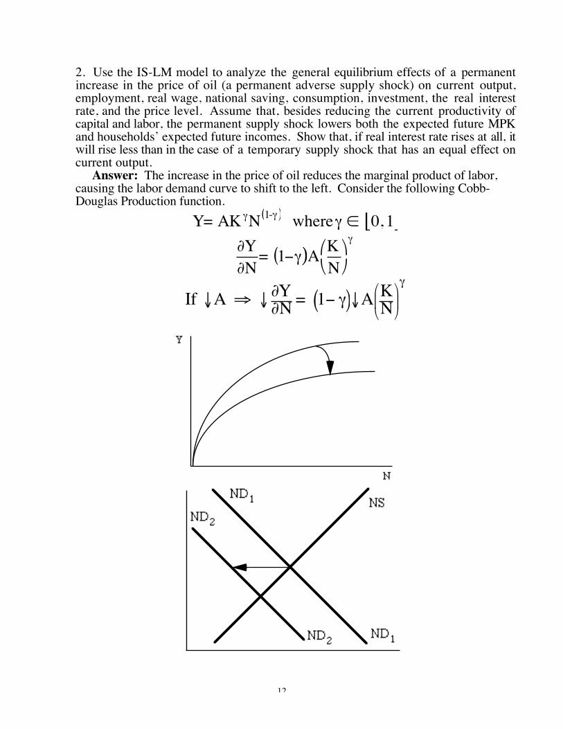
2. Use the IS-LM model to analyze the general equilibrium effects of a permanentincrease in the price of oil (a permanent adverse supply shock) on current output,employment, real wage, national saving, consumption, investment, the real interestrate, and the price level. Assume that, besides reducing the current productivity ofcapital and labor, the permanent supply shock lowers both the expected future MPKand households’ expected future incomes. Show that, if real interest rate rises at all, itwill rise less than in the case of a temporary supply shock that has an equal effect oncurrent output.

Answer: The increase in the price of oil reduces the marginal product of labor,causing the labor demand curve to shift to the left. Consider the following Cobb-Douglas Production function.

Y= AK γN 1-γ( ) where γ ∈ 0, 1[ ]∂Y∂N

= 1−γ( )A KN

γ

If ↓A ⇒ ↓∂Y∂N = 1− γ( )↓A KN

γ

13

Decrease in the quantity of labor supplied:

↓N ⇒ ↓Y =AF K ,↓N

Full Employment Output Changes: Consider a temporary adverse supply shockfirst

14

A temporary adverse supply shock, reduces the full employment level ofoutput. Does the IS curve shift? NO. This is a movement along the IS curve. Whathappens to national savings when Y changes? ANS:

↓Y ⇒ ↓Sd = ↓Y− ↓Cd − G

↓Y is precisely how we derived the IS schedule. Thus IS does not change and theshift in the FE line is along a stable IS curve.

At point A: Initial general equilibrium point. After the adverse supply shock, this isthe short run equilibrium, where IS and LM intersect. Here the goods market is inequilibrium since aggregate quantities of goods supplied equal the quantitiesdemanded. Recall that firms always produce more output as aggregate quantities ofgoods demanded rises. But notice that the firms, though, they are meeting thisdemand, they are producing more output than the new full-employment level ofoutput. The full employment level of output fell when FE shifted to the left. The full-employment level of output is determined by firms’ labor and capital hiring decisions. But, at point A, firms’ are producing more than their profit maximizing levels ofoutput. So at point A

Y < Cd+Id+GThus point A cannot be a long run equilibrium. But how will this adjust? Recall,that we have taken prices to be fixed. But now that will no longer be the case.Firms will raise their prices since the aggregate quantity of goods demanded exceedswhat firms want to produce.

Price level rises:

⇒ ↓ Ms

↑P

=↓L Y, ↑r + πe

⇒ real money supply shifts to the left along a stable money demand function

15

How do we explain the movement along the IS curve?

↓Y ⇒ ↓Cd ⇒ ↓Sd=↓Y−↓Cd−G

⇒ savings shifts leftward

16

After the adjustment

When the shock is temporary there is no impact on future output or the futuremarginal product of capital, so the IS curve does not shift. In that case the pricelevel increases to restore equilibrium. In that case, the real interest rateunambiguously increases.

KEY POINT: Under a permanent shock, the IS curve shifts down, so the rise inthe real interest rate is less than in the case of a temporary shock, and the real interestrate can even decline.

We have provided the answer to the case of a temporary supply shock.

17

Now consider the case of a permanent supply shock.

The adverse supply shock results in a shift to the left of the full-employment line, asboth employment and productivity decline.

Because the shock is permanent, it reduces future output and reduces the futuremarginal product of capital, both of which result in a downward shift of the IScurve.

The new equilibrium is located at the intersection of the new IS curve and the newFE line.

If, as we have drawn the figure, this intersection lies above and to the left of theoriginal LM curve, the price level will increase and shift the LM curve upward to passthrough the new equilibrium point.

The result is an increase in the price level, but an ambiguous effect on the realinterest rate.

Since output is lower, consumption is lower.

Since the effect on the real interest rate is ambiguous, the effect on saving andinvestment are ambiguous as well, though the fall in the future marginal product ofcapital would tend to reduce investment.

18

3. Suppose that the price level is fixed in the short run so that the economy doesn’treach general equilibrium immediately after a change in the economy. For each of thefollowing changes, what are the short-run effects on the real interest rate and output?Assume that, when the economy is in disequilibrium, only the labor market is out ofequilibrium; assume also that for a short period firms are willing to produce enoughoutput to meet the aggregate demand for output.

a. A decrease in the expected rate of inflation.

Answer: If ↓πethen real money demand rises, i.e., shifts rightward .

Adjustment Story: at the old interest rate, the quantity of money demandedexceeds the supply of money. Agents sell nonmonetary assets, driving their pricesdown and their real returns (the real interest rate paid on the asset) up. As the realinterest rate rises, individuals find money less and less attractive relative to thenonmonetary asset . Eventually the interest rate will rise so high that the excesssupply of money and the excess demand for nonmonetary assets are zero.

↑r ⇒↑Md = P↑L Y, ↑ r + π e( ) ⇒ movement along new money demand schedule.

Where the LM function is

LM r, Y; πe , P, Ms, im, W, risk of nonmonetary assets, risk of money,

efficiency of payments technologies , liquidity of alternative assets

19

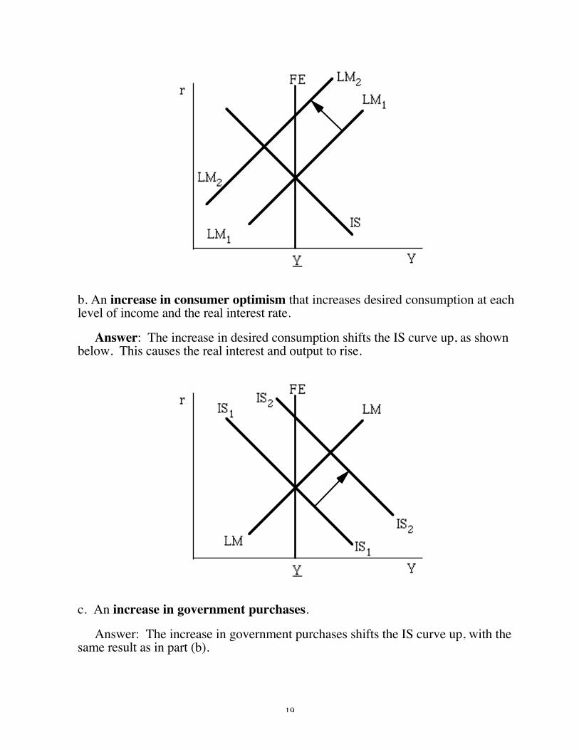
b. An increase in consumer optimism that increases desired consumption at eachlevel of income and the real interest rate.

Answer: The increase in desired consumption shifts the IS curve up, as shownbelow. This causes the real interest and output to rise.

c. An increase in government purchases.

Answer: The increase in government purchases shifts the IS curve up, with thesame result as in part (b).

20

d. An increase in lump-sum taxes, with no change in government purchases(consider both the case in which Ricardian equivalence holds and the case in which itdoesn’t).

Answer: If Ricardian equivalence holds, the increase in taxes has no effect.If Ricardian equivalence doesn’t hold, the increase in taxes reduces consumptionspending and the IS curve shifts down. Both the real interest rate and output decline.

e. A scientific breakthrough increases the expected future MPK.

Answer: An increase in the expected future marginal productivity of capital shiftsthe IS curve up, with the same result as in part (b).