identi cation of fracture toughness for discrete damage...

Applied Composite Materials, 0():xxx-xxx, 2014.

Identification of Fracture Toughness forDiscrete Damage Mechanics Analysis of

Glass-Epoxy Laminates

E. J. Barbero1 and F. A. Cosso 2

Mechanical and Aerospace Engineering, West Virginia University,Morgantown, WV 26506-6106, USA

and

X. Martinez 3

Technical Univeristy of Catalonia (UPC), Spain

Abstract

A methodology for determination of the intralaminar fracture toughness is presented, based onfitting discrete damage mechanics (DDM) model predictions to available experimental data. DDMis constitutive model that, when incorporated into commercial finite element software via usermaterial subroutines, is able to predict intralaminar transverse and shear damage initiation andevolution in terms of the fracture toughness of the composite. The applicability of the DDM modelis studied by comparison to available experimental data for Glass-Epoxy laminates. Sensitivity ofthe DDM model to h- and p-refinement is studied. Also, the effect of in-situ correction of strengthis highlighted.

Keywords

A. Polymer-matrix composites (PMCs); B. Transverse cracking; C. Damage mechanics; C. Finiteelement analysis (FEA); Parameter Identification.

1 Introduction

Prediction of damage initiation and accumulation in polymer matrix, laminated composites is ofgreat interest for the design, production, certification, and monitoring of an increasingly largevariety of structures. Matrix cracking due to transverse tensile and shear deformations is normallythe first mode of damage and, if left unmitigated often leads to other modes such as delamination,fiber failure of adjacent laminas due to load redistribution, and reduction of the shear stiffness, whichin turn deteriorates the longitudinal compressive strength of the composite [1]. Furthermore, matrix

1Corresponding author. The final publication is available at http://dx.doi.org/10.1007/s10443-013-9359-y2Graduate Research Assistant.3Professor (UPC) and Researcher (CIMNE)

1

http://dx.doi.org/10.1007/s10443-013-9359-y

Applied Composite Materials, 0():xxx-xxx, 2014. 2

cracking leads to increased permeability and exposes the fibers to deleterious environmental attack,which in the case of Glass and polymeric fibers, may lead to unacceptable material degradation.

As any other fracture process, transverse matrix cracking is defined by failure onset and prop-agation. The simplest way to address matrix cracking is by limiting the design allowable to thematerial strength at failure onset. Many models follow this approach [2, 3]. Most of them addresstransverse matrix cracking together with other failure mechanisms such as matrix compressive fail-ure, fibre tensile rupture or fibre compression failure. These models can be included in a finiteelement code using the ply discount method [4, § 7.3.1].

More sophisticated models are capable of predicting damage onset and propagation. In [5–7],the response of each lamina is obtained from a meso-model that couples the behaviour of a singlelayer and an interlaminar layer. The first layer uses a damage model capable of differentiatingbetween tensile and compression loads, thus accounting for transverse matrix crack effects. Thesecond layer uses a two dimensional damage model that only takes into account stresses that leadto delamination failure. Parameter identification is described in [6,7] and validation with open-holetensile tests on quasi-isotropic laminates is given in [8].

Another approach to simulate the onset and propagation of transverse matrix cracking, aswell as other failure mechanisms, is serial-parallel mixing theory [9]. This formulation obtains thecomposite response from the constitutive performance of its constituents, usually matrix and fibre,each one of them simulated with its own constitutive law. With this theory it is possible to useany given non-linear material model, such as damage or plasticity, to characterize the compositecomponents. The correct determination of failure onset and propagation depends on the capacityand accuracy of the model used. Examples of of this formulation are shown in [10–12].

When looking into the models developed specifically to address the phenomenon of transversematrix cracking, most of them establish a relation between the available strain energy of the mate-rial and the density of matrix cracks [13–23]. Following this approach, [17, 19] uses finite fracturemechanics to obtain the energy release rate required to double the crack density, with the ap-parition of a new crack between two existing cracks. This model was improved with the conceptof incremental and continuous variation of crack density [20], showing that the calculation of theenergy release rate required to crack propagation is more accurate if crack density is assumedto grow continuously, instead of doubling at each increment. Further, the equivalent constrainedmodel (ECM) [21,22], defines a law that provides the evolution of stiffness as matrix crack densityincreases. Again, the increment of matrix cracks depends on the strain energy release rate.

Some of the above mentioned formulations provide analytical expressions that can be used toobtain the mechanical response for simple geometry and load configurations. However, it is oftennecessary to include the constitutive model into Finite Element Analysis Software. Some modelshave been included in commercial FEM software [24–26], others that are available as plugins forexisting FEA software [27, 28], or as user programmable features, including UMAT, UGENS [29]or USERMAT [30].

In this manuscript, it is proposed to use Discrete Damage Mechanics (DDM) for the simulationof transverse matrix cracking. Briefly, DDM [31] is a constitutive model that is objective [32], i.e.,the predictions are not affected by the element size or type (linear, quadratic, etc.). Furthermore,only two material parameters, the fracture toughness in modes I and II, are required to predictboth initiation and evolution of transverse and shear damage.

Since fracture toughness is used to predict damage initiation (transverse and shear strengths arenot used) DDM does not require in-situ correction of strength. No hardening/softening parametersare required either, which avoids costly experimentation that would otherwise be required to de-termine them. Also, as it is shown in this work, DDM parameters can be identified for Glass fibercomposites. This is not easily done with continuum damage mechanics (CDM) models because


their state variables (damage variables), are not direclty measurable [33]. As a result, CDM’s ma-terial parameters must be identified using a macroscopic effect, such as the loss of stiffness, whichin most cases is difficult to measure [34].

Finally, DDM has also the advantage that it is already available to be used in commercialFEA environments such as Abaqus4 [26] and ANSYS/Mechanical5 [35], in the form of UMAT,UGENS [29], and USERMAT [30]. It is also possible to obtain the composite response to uniaxialtensile loads with the webpage application [36, Cadec/Chapters/Damage/DDM].

The objective of this manuscript is to propose a methodology to identify the fracture toughnessusing available experimental data. Once the DDM model parameters are identified, validation ispresented by predicting other, independent results, and conclusions are drawn about the applica-bility of the model.

Standards exist for measuring interlaminar (not intralaminar) fracture toughness in mode I(ASTM D5528) and proposed methods exists for mode II [37, 38], but no standard test methodexist to measure intralaminar fracture toughness. Thus, a method to identify the DDM modelparameters is necessary.

2 Discrete Damage Mechanics

Given the crack density λ and the shell strain ε, κ, DDM updates the state variable, i.e., the crackdensity, and calculates the shell stress resultants N,M , and tangent stiffness matrix AT , BT , DT ,all of them functions of crack density. The crack density λ is an array containing the crack densityfor all laminas at an integration point of the shell element. Since the strain is conjugate to the shellstress resultant, DDM provides a constitutive model that can be implemented as a user materialsubroutine (UMAT, VUMAT, USERMAT) [30, usermatps-901] for flat plane stress elements andas a user general section (UGENS) for curved shell elements [29, ugens-std].

2.1 Description of the Model

In DDM, damage initiation and evolution are controlled by a single equation representing theGriffith’s criterion for an intralaminar crack, i.e., the undamaging domain is defined by

g(ε, λ) = max

[GI(ε, λ)

GIC,GII(ε, λ)

GIIC

]− 1 ≤ 0 (1)

where GI , GII are the strain energy release rates (ERR) in modes I and II, calculated with (14)-(15),and GIC , GIIC are the invariant material properties representing the energy necessary to create anew crack. We shall see that for fixed strain, both are decreasing functions of λ and thus (1)exhibits strain-hardening for increasing λ, resulting in stress-softening as a function of strain.

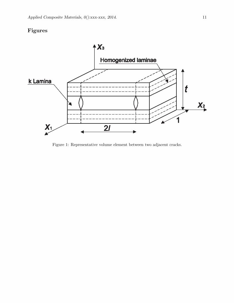
DDM calculates GI , GII solving the 3D equilibrium equations in the RVE (Fig. 1)

∇ · σ − f = 0 (2)

reduced to 2D by the following approximations. The u3 component of displacement is eliminatedby assuming a state of plane stress for symmetric laminates under membrane loads,

σ3 = 0 ;∂u3∂xi

= 0 with i = 1, 2 (3)

4Abaqus and Simulia are trademarks or registered trademarks of Dassault Systemes or its subsidiaries in theUnited States and/or other countries.

5Ansys R© is a registered trademark of ANSYS Inc.


Then, (2) are written in terms of the average of the displacements over the thickness of eachlamina, defined as

u(k)i =

∫ tk/2

−tk/2ui(z)dz (4)

where tk is the thickness of lamina k. Next, the intralaminar shear stress is assumed to be linear ineach lamina k, from the interface between laminas k − 1 and k (denoted k − 1, k) to the interfacebetween laminas k and k + 1,

τ(k)j3 (x3) = τk−1,kj3 +

(τk,k+1j3 − τk−1,kj3

) x3 − xk−1,k3

tk; j = 1, 2 (5)

where x3 is the coordinate along the thickness of the laminate, and xk−1,k3 is the coordinate ofthe interface between laminas k − 1 and k. Therefore, the 3D equilibrium equations (2) reduceto a system of 2N partial differential equations (PDE) in two dimensions, in terms of averagedisplacements, with two equations per lamina.

Periodically spaced cracks, which propagate suddenly in a unstable fashion through the thicknessof the lamina and along the fiber direction are assumed [39], [4, § 7.2.1]. Therefore, a representativevolume element (RVE) is chosen spanning the laminate thickness between two adjacent cracks(Fig. 1). The crack density is inversely proportional to the length 2l of the RVE,

λ = 1/2l (6)

Thus, crack density is represented in the model by the length of the RVE. Since the RVE isindependent of the finite element discretization, and the constitutive model is formulated in termsof displacements (not strains), the constitutive model is objective, without needing a characteristiclength. By plotting the reaction force vs. applied displacement on the boundary, the numericalresults presented in this work corroborate the objectivity of the model.

The PDE system is complemented by the following boundary conditions. The surface of thecracks in lamina c, located at x = ±l, are free boundaries, and thus subject to zero stress

1/2

∫−1/2

σ(c)j (x1, l) dx1 = 0 ; j = 2, 6 (7)

All laminas m = 1..N with m 6= c, that is, excluding the cracking lamina c, undergo the samedisplacement at the boundaries (−l, l) when subjected to a membrane state of strain. Taking anarbitrary lamina r 6= c as a reference, the other displacements are

u(m)j (x1,±l) = u

(r)j (x1,±l) ; ∀m 6= k ; j = 1, 2 (8)

Finally, the stress resultant from the internal stress equilibrates the applied load. In the directionparallel to the surface of the cracks (fiber direction x1) the load is supported by all the laminas inthe laminate,

1

2l

N∑k=1

tk

l∫−l

σ(k)1 (1/2, x2)dx2 = N1 (9)


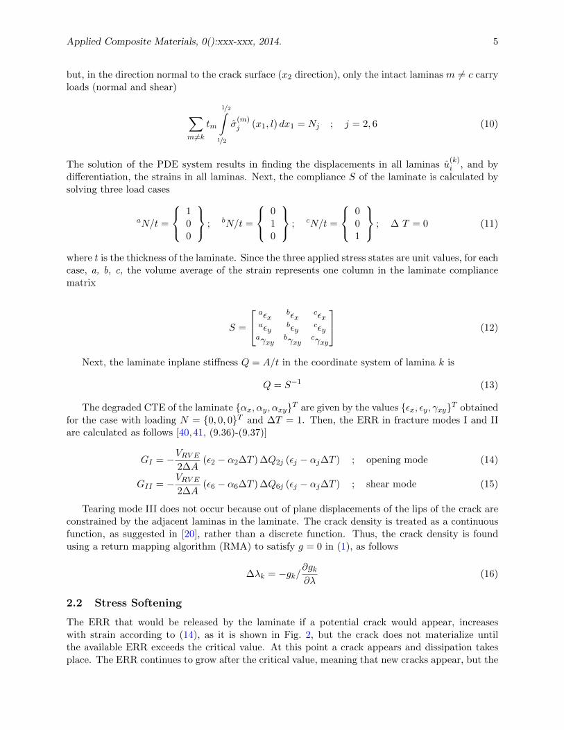
but, in the direction normal to the crack surface (x2 direction), only the intact laminas m 6= c carryloads (normal and shear)

∑m 6=k

tm

1/2∫1/2

σ(m)j (x1, l) dx1 = Nj ; j = 2, 6 (10)

The solution of the PDE system results in finding the displacements in all laminas u(k)i , and by

differentiation, the strains in all laminas. Next, the compliance S of the laminate is calculated bysolving three load cases

aN/t =

100

; bN/t =

010

; cN/t =

001

; ∆ T = 0 (11)

where t is the thickness of the laminate. Since the three applied stress states are unit values, for eachcase, a, b, c, the volume average of the strain represents one column in the laminate compliancematrix

S =

aεxbεx

cεxaεy

bεycεy

aγxybγxy

cγxy

(12)

Next, the laminate inplane stiffness Q = A/t in the coordinate system of lamina k is

Q = S−1 (13)

The degraded CTE of the laminate {αx, αy, αxy}T are given by the values {εx, εy, γxy}T obtainedfor the case with loading N = {0, 0, 0}T and ∆T = 1. Then, the ERR in fracture modes I and IIare calculated as follows [40,41, (9.36)-(9.37)]

GI = −VRV E2∆A

(ε2 − α2∆T ) ∆Q2j (εj − αj∆T ) ; opening mode (14)

GII = −VRV E2∆A

(ε6 − α6∆T ) ∆Q6j (εj − αj∆T ) ; shear mode (15)

Tearing mode III does not occur because out of plane displacements of the lips of the crack areconstrained by the adjacent laminas in the laminate. The crack density is treated as a continuousfunction, as suggested in [20], rather than a discrete function. Thus, the crack density is foundusing a return mapping algorithm (RMA) to satisfy g = 0 in (1), as follows

∆λk = −gk/∂gk∂λ

(16)

2.2 Stress Softening

The ERR that would be released by the laminate if a potential crack would appear, increaseswith strain according to (14), as it is shown in Fig. 2, but the crack does not materialize untilthe available ERR exceeds the critical value. At this point a crack appears and dissipation takesplace. The ERR continues to grow after the critical value, meaning that new cracks appear, but the


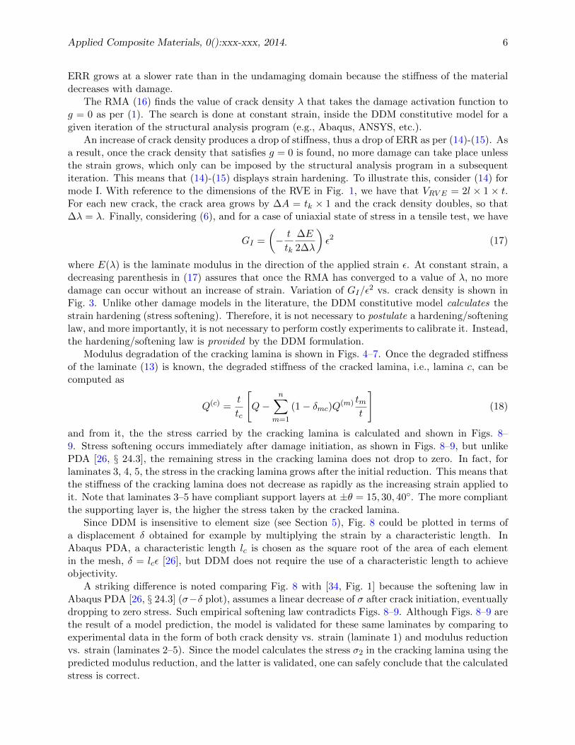
ERR grows at a slower rate than in the undamaging domain because the stiffness of the materialdecreases with damage.

The RMA (16) finds the value of crack density λ that takes the damage activation function tog = 0 as per (1). The search is done at constant strain, inside the DDM constitutive model for agiven iteration of the structural analysis program (e.g., Abaqus, ANSYS, etc.).

An increase of crack density produces a drop of stiffness, thus a drop of ERR as per (14)-(15). Asa result, once the crack density that satisfies g = 0 is found, no more damage can take place unlessthe strain grows, which only can be imposed by the structural analysis program in a subsequentiteration. This means that (14)-(15) displays strain hardening. To illustrate this, consider (14) formode I. With reference to the dimensions of the RVE in Fig. 1, we have that VRV E = 2l × 1 × t.For each new crack, the crack area grows by ∆A = tk × 1 and the crack density doubles, so that∆λ = λ. Finally, considering (6), and for a case of uniaxial state of stress in a tensile test, we have

GI =

(− t

tk

∆E

2∆λ

)ε2 (17)

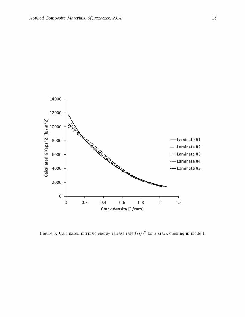
where E(λ) is the laminate modulus in the direction of the applied strain ε. At constant strain, adecreasing parenthesis in (17) assures that once the RMA has converged to a value of λ, no moredamage can occur without an increase of strain. Variation of GI/ε

2 vs. crack density is shown inFig. 3. Unlike other damage models in the literature, the DDM constitutive model calculates thestrain hardening (stress softening). Therefore, it is not necessary to postulate a hardening/softeninglaw, and more importantly, it is not necessary to perform costly experiments to calibrate it. Instead,the hardening/softening law is provided by the DDM formulation.

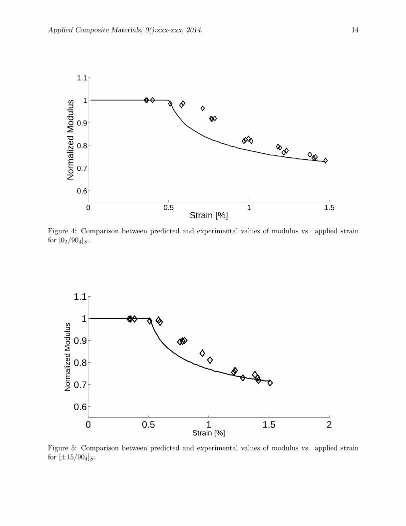
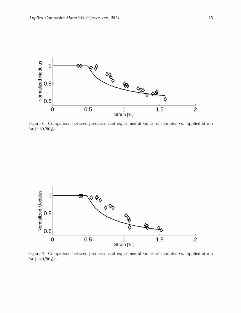
Modulus degradation of the cracking lamina is shown in Figs. 4–7. Once the degraded stiffnessof the laminate (13) is known, the degraded stiffness of the cracked lamina, i.e., lamina c, can becomputed as

Q(c) =t

tc

[Q−

n∑m=1

(1− δmc)Q(m) tmt

](18)

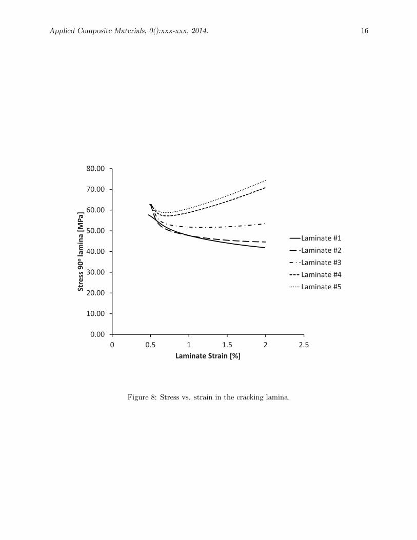
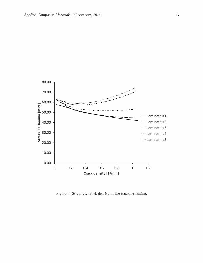
and from it, the the stress carried by the cracking lamina is calculated and shown in Figs. 8–9. Stress softening occurs immediately after damage initiation, as shown in Figs. 8–9, but unlikePDA [26, § 24.3], the remaining stress in the cracking lamina does not drop to zero. In fact, forlaminates 3, 4, 5, the stress in the cracking lamina grows after the initial reduction. This means thatthe stiffness of the cracking lamina does not decrease as rapidly as the increasing strain applied toit. Note that laminates 3–5 have compliant support layers at ±θ = 15, 30, 40◦. The more compliantthe supporting layer is, the higher the stress taken by the cracked lamina.

Since DDM is insensitive to element size (see Section 5), Fig. 8 could be plotted in terms ofa displacement δ obtained for example by multiplying the strain by a characteristic length. InAbaqus PDA, a characteristic length lc is chosen as the square root of the area of each elementin the mesh, δ = lcε [26], but DDM does not require the use of a characteristic length to achieveobjectivity.

A striking difference is noted comparing Fig. 8 with [34, Fig. 1] because the softening law inAbaqus PDA [26, § 24.3] (σ−δ plot), assumes a linear decrease of σ after crack initiation, eventuallydropping to zero stress. Such empirical softening law contradicts Figs. 8–9. Although Figs. 8–9 arethe result of a model prediction, the model is validated for these same laminates by comparing toexperimental data in the form of both crack density vs. strain (laminate 1) and modulus reductionvs. strain (laminates 2–5). Since the model calculates the stress σ2 in the cracking lamina using thepredicted modulus reduction, and the latter is validated, one can safely conclude that the calculatedstress is correct.


3 Strength Criterion

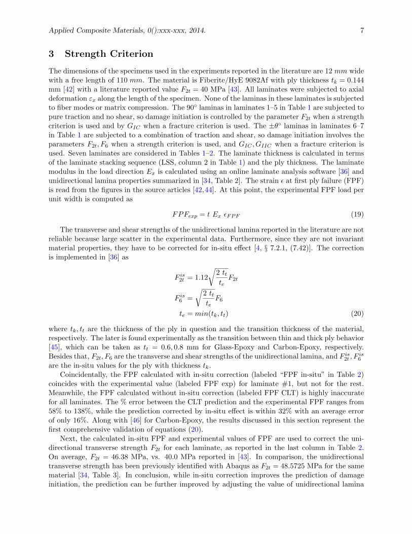
The dimensions of the specimens used in the experiments reported in the literature are 12 mm widewith a free length of 110 mm. The material is Fiberite/HyE 9082Af with ply thickness tk = 0.144mm [42] with a literature reported value F2t = 40 MPa [43]. All laminates were subjected to axialdeformation εx along the length of the specimen. None of the laminas in these laminates is subjectedto fiber modes or matrix compression. The 90◦ laminas in laminates 1–5 in Table 1 are subjected topure traction and no shear, so damage initiation is controlled by the parameter F2t when a strengthcriterion is used and by GIC when a fracture criterion is used. The ±θ◦ laminas in laminates 6–7in Table 1 are subjected to a combination of traction and shear, so damage initiation involves theparameters F2t, F6 when a strength criterion is used, and GIC , GIIC when a fracture criterion isused. Seven laminates are considered in Tables 1–2. The laminate thickness is calculated in termsof the laminate stacking sequence (LSS, column 2 in Table 1) and the ply thickness. The laminatemodulus in the load direction Ex is calculated using an online laminate analysis software [36] andunidirectional lamina properties summarized in [34, Table 2]. The strain ε at first ply failure (FPF)is read from the figures in the source articles [42,44]. At this point, the experimental FPF load perunit width is computed as

FPFexp = t Ex εFPF (19)

The transverse and shear strengths of the unidirectional lamina reported in the literature are notreliable because large scatter in the experimental data. Furthermore, since they are not invariantmaterial properties, they have to be corrected for in-situ effect [4, § 7.2.1, (7.42)]. The correctionis implemented in [36] as

F is2t = 1.12

√2 ttteF2t

F is6 =

√2 ttteF6

te = min(tk, tt) (20)

where tk, tt are the thickness of the ply in question and the transition thickness of the material,respectively. The later is found experimentally as the transition between thin and thick ply behavior[45], which can be taken as tt = 0.6, 0.8 mm for Glass-Epoxy and Carbon-Epoxy, respectively.Besides that, F2t, F6 are the transverse and shear strengths of the unidirectional lamina, and F is2t , F

is6

are the in-situ values for the ply with thickness tk.Coincidentally, the FPF calculated with in-situ correction (labeled “FPF in-situ” in Table 2)

coincides with the experimental value (labeled FPF exp) for laminate #1, but not for the rest.Meanwhile, the FPF calculated without in-situ correction (labeled FPF CLT) is highly inaccuratefor all laminates. The % error between the CLT prediction and the experimental FPF ranges from58% to 138%, while the prediction corrected by in-situ effect is within 32% with an average errorof only 16%. Along with [46] for Carbon-Epoxy, the results discussed in this section represent thefirst comprehensive validation of equations (20).

Next, the calculated in-situ FPF and experimental values of FPF are used to correct the uni-directional transverse strength F2t for each laminate, as reported in the last column in Table 2.On average, F2t = 46.38 MPa, vs. 40.0 MPa reported in [43]. In comparison, the unidirectionaltransverse strength has been previously identified with Abaqus as F2t = 48.5725 MPa for the samematerial [34, Table 3]. In conclusion, while in-situ correction improves the prediction of damageinitiation, the prediction can be further improved by adjusting the value of unidirectional lamina


strength (in this case from 40 to 46.38 MPa) to better match the experimental values of damageinitiation.

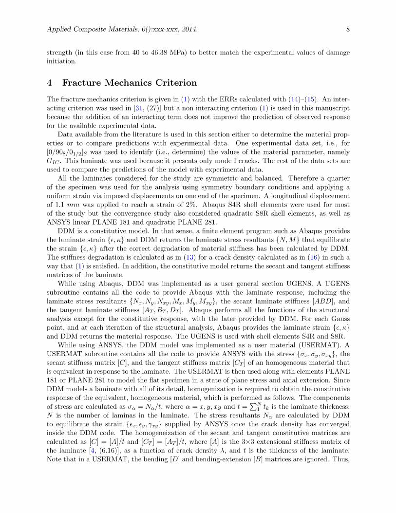
4 Fracture Mechanics Criterion

The fracture mechanics criterion is given in (1) with the ERRs calculated with (14)–(15). An inter-acting criterion was used in [31, (27)] but a non interacting criterion (1) is used in this manuscriptbecause the addition of an interacting term does not improve the prediction of observed responsefor the available experimental data.

Data available from the literature is used in this section either to determine the material prop-erties or to compare predictions with experimental data. One experimental data set, i.e., for[0/908/01/2]S was used to identify (i.e., determine) the values of the material parameter, namelyGIC . This laminate was used because it presents only mode I cracks. The rest of the data sets areused to compare the predictions of the model with experimental data.

All the laminates considered for the study are symmetric and balanced. Therefore a quarterof the specimen was used for the analysis using symmetry boundary conditions and applying auniform strain via imposed displacements on one end of the specimen. A longitudinal displacementof 1.1 mm was applied to reach a strain of 2%. Abaqus S4R shell elements were used for mostof the study but the convergence study also considered quadratic S8R shell elements, as well asANSYS linear PLANE 181 and quadratic PLANE 281.

DDM is a constitutive model. In that sense, a finite element program such as Abaqus providesthe laminate strain {ε, κ} and DDM returns the laminate stress resultants {N,M} that equilibratethe strain {ε, κ} after the correct degradation of material stiffness has been calculated by DDM.The stiffness degradation is calculated as in (13) for a crack density calculated as in (16) in such away that (1) is satisfied. In addition, the constitutive model returns the secant and tangent stiffnessmatrices of the laminate.

While using Abaqus, DDM was implemented as a user general section UGENS. A UGENSsubroutine contains all the code to provide Abaqus with the laminate response, including thelaminate stress resultants {Nx, Ny, Nxy,Mx,My,Mxy}, the secant laminate stiffness [ABD], andthe tangent laminate stiffness [AT , BT , DT ]. Abaqus performs all the functions of the structuralanalysis except for the constitutive response, with the later provided by DDM. For each Gausspoint, and at each iteration of the structural analysis, Abaqus provides the laminate strain {ε, κ}and DDM returns the material response. The UGENS is used with shell elements S4R and S8R.

While using ANSYS, the DDM model was implemented as a user material (USERMAT). AUSERMAT subroutine contains all the code to provide ANSYS with the stress {σx, σy, σxy}, thesecant stiffness matrix [C], and the tangent stiffness matrix [CT ] of an homogeneous material thatis equivalent in response to the laminate. The USERMAT is then used along with elements PLANE181 or PLANE 281 to model the flat specimen in a state of plane stress and axial extension. SinceDDM models a laminate with all of its detail, homogenization is required to obtain the constitutiveresponse of the equivalent, homogeneous material, which is performed as follows. The componentsof stress are calculated as σα = Nα/t, where α = x, y, xy and t =

∑N1 tk is the laminate thickness;

N is the number of laminas in the laminate. The stress resultants Nα are calculated by DDMto equilibrate the strain {εx, εy, γxy} supplied by ANSYS once the crack density has convergedinside the DDM code. The homogeneization of the secant and tangent constitutive matrices arecalculated as [C] = [A]/t and [CT ] = [AT ]/t, where [A] is the 3×3 extensional stiffness matrix ofthe laminate [4, (6.16)], as a function of crack density λ, and t is the thickness of the laminate.Note that in a USERMAT, the bending [D] and bending-extension [B] matrices are ignored. Thus,


the USERMAT can be used only to model plates under membrane loads, while the UGENS can beused to model the combined membrane-flexural behavior of curved shells.

The difference between USERMAT (or UMAT) and UGENS implementation highlights an ad-vantage of DDM over local constitutive models. Most damage constitutive models in the literatureare local, in the sense that they model the constitutive behavior σ = σ(ε, λ), at a material pointinside a lamina (e.g., Simpson integration point inside a lamina), without direct coupling with thedamage taking place simultaneously in other laminas. In contrast, DMM takes into account alllaminas simultaneously in the RVE (see § 2.1 and Fig. 1). Local models can be implemented usingUSERMAT (or UMAT) to be used at the lamina level, but in doing so, the local models update thestate variables (e.g., crack density) in a given lamina using the values of the state variables for theremaining laminas from a prior iteration of the structural analysis program. On the other hand,DDM needs to calculate the entire laminate at once, thus requiring a UGENS implementation (orthe homogenization scheme used for ANSYS USERMAT). Furthermore, the fact that local modelsσ = σ(ε, λ) implicitly affect the volume around an integration point, causes the solution to be meshdependent, thus requiring additional steps to attain objectivity [32].

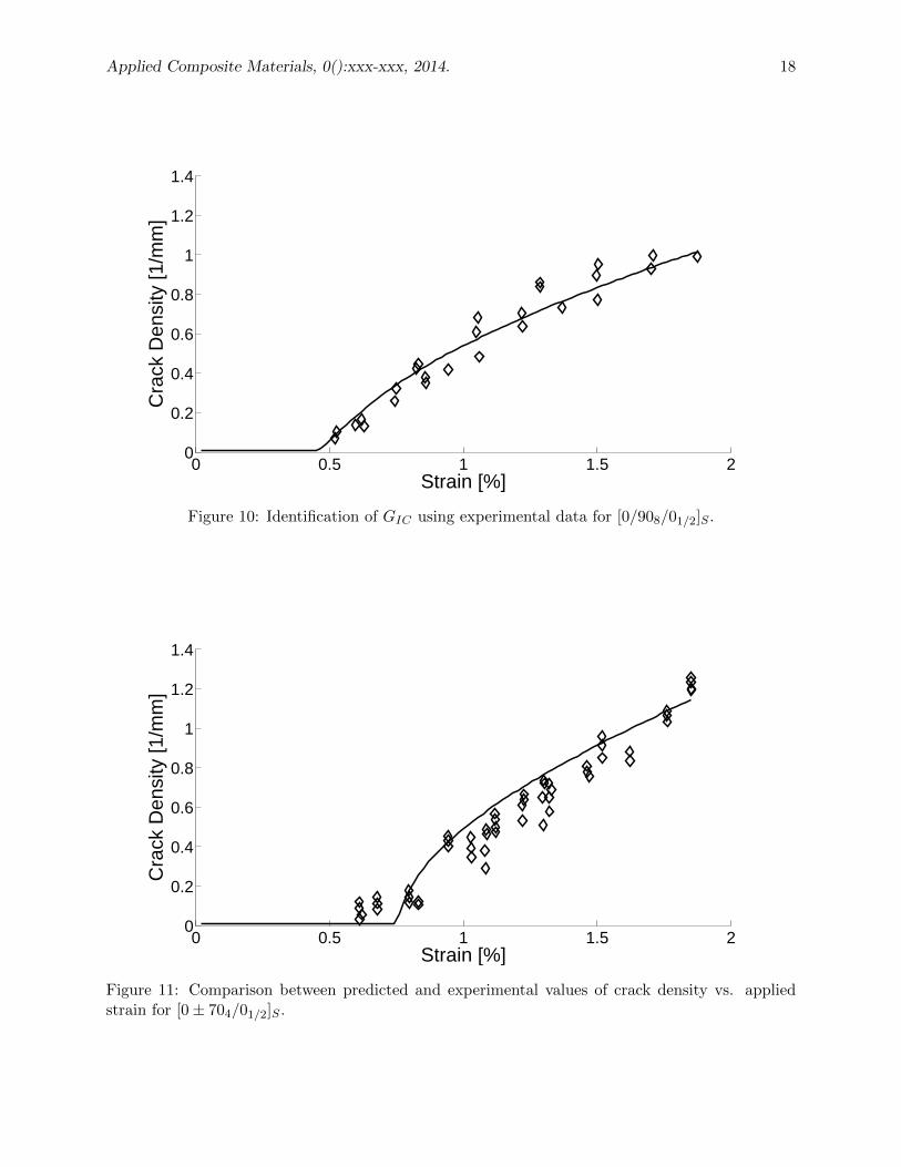
Using the USERMAT/UGENS implementation described above, the value of critical energyrelease rate GIC was identified in such a way that the DDM model provides a best fit to theexperimental crack density λ vs. stress σx for laminate 1 in Tables 1–2. The experimental dataand the fitted DDM model results are shown in Fig. 10.

The error was calculated using the usual formula

Error =1

n

√√√√ n∑i=1

[χmodel(ξi)− χexperim(ξi)]2

(21)

where χmodel, χexperim are the predicted and experimental values of the dependent variable, respec-tively; ξi is the test progress indicator, be it stress or strain depending on how the experimentaldata is reported in the literature, and n is the number of experimental data points available. Thedependent variables used in this study include crack density λ, laminate modulus Ex, and laminatePoisson’s ratio νxy.

By adjusting the parameters GIC , the minimization algorithm converges to a global minimum.A MATLAB script was executed to look for the minimum error (21), by repeatedly executingAbaqus with parameters varying as per the Simplex method [47]. The converged values of GIC =253.5 J/m2 was obtained for Fiberite/HyE 9082Af. The best fit can be seen in Fig. 10. The error,i.e., the difference between the prediction and experimental data points, is very small and is dueonly to the dispersion of the experimental results.

For laminates 1, 6, and 7 [44], the measured property is crack density λ and the independentvariable is the applied laminate strain εx. For laminates 2–5 [42], the independent variable is againstrain but the dependent variable is the normalized modulus and the normalized Poisson’s ratio.

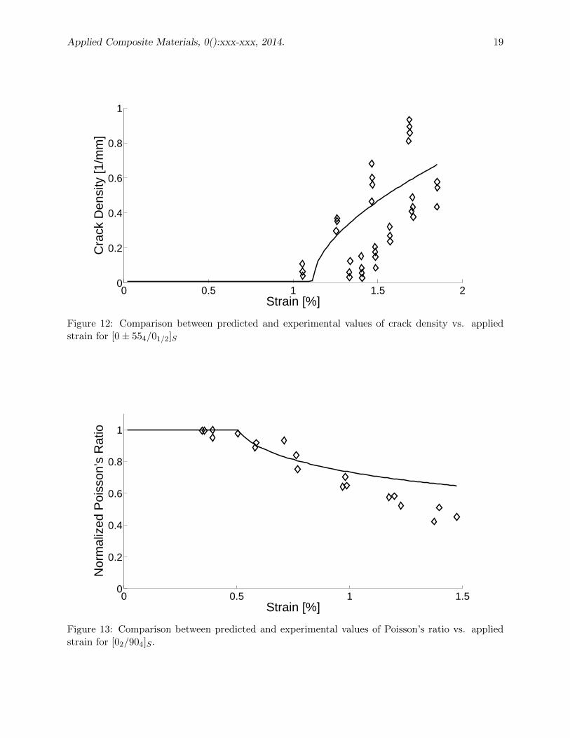
Predicted crack density vs. applied strain for laminates 6 and 7 are shown in Figs. 11 and12, respectively; both presenting good agreement between model and the experiments. In bothcases, mode I fracture was assumed to be dominant, which is corroborated by the quality of thepredictions.

Predicted laminate modulus Ex vs. applied strain for laminates 2–5, are shown in Figs. 4–7. Inall cases, both damage onset and evolution are predicted quite well.

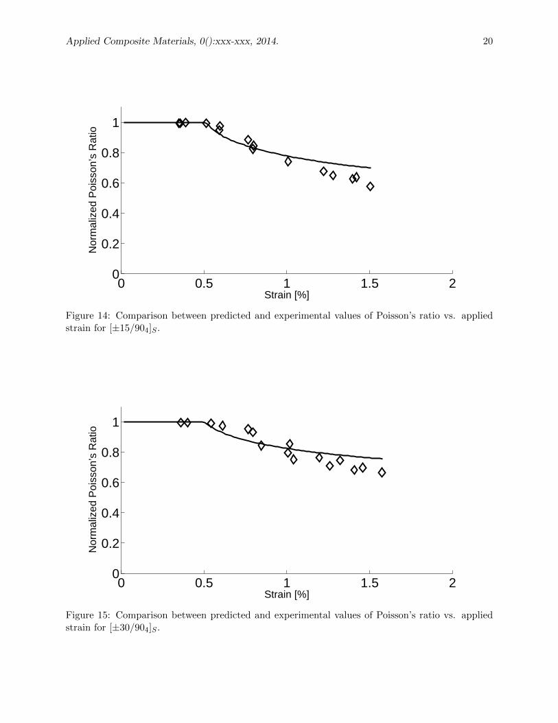
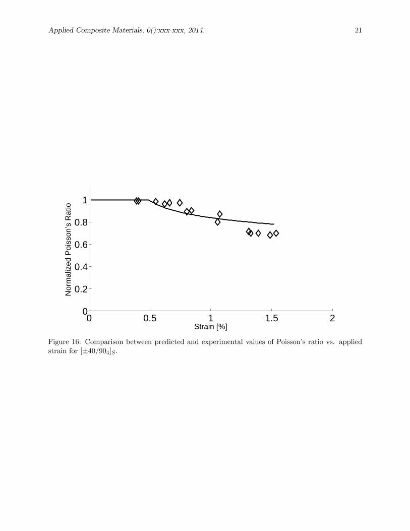
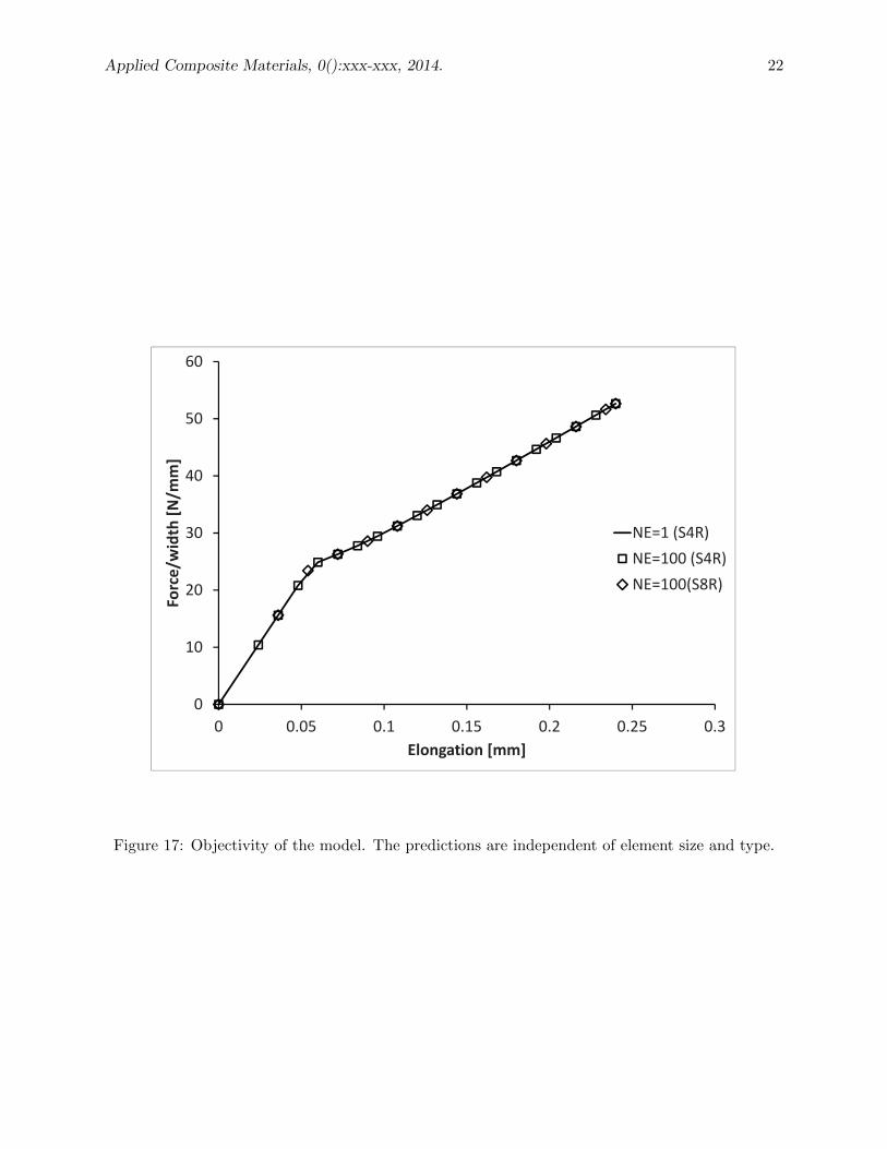
Predicted Poisson’s ratio νxy vs. applied strain for laminates 2–5, are shown in Figs. 13–16. Inall cases, both damage onset and evolution are predicted quite well.


5 Convergence

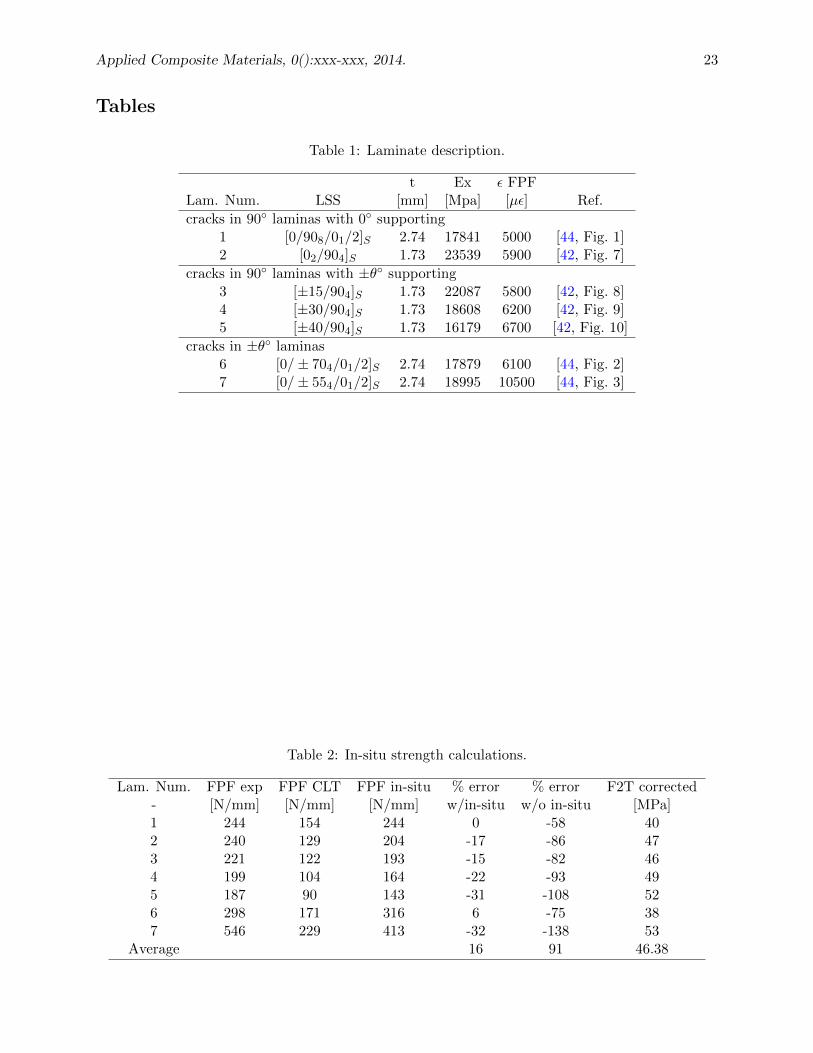
In this section we assess the sensitivity of the DDM model to h- and p-refinement, realized by meshrefinement and by changing the element type, respectively. Reaction force vs. applied displacementare reported in Fig. 17 using two discretizations, namely 1 and 100 elements of type S4R in Abaqus,thus demonstrating h-refinement. Furthermore, the analysis is repeated using elements S8R inAbaqus, thus achieving p-refinement.

Since a uniform state of strain is applied, h- and/or p-refinement is not necessary to converge ona solution, unless the constitutive model were mesh dependent (see [34, Figs. 14–15]). Objectivityof the DDM constitutive model is verified by showing that the results are not affected by elementsize or type, namely linear S4R or quadratic S8R (Fig. 17). Abaqus linear S4R elements were usedwhile adjusting the fracture toughness GIC , but the predictions are not affected if the element ischanged to Abaqus quadratic S8R, or ANSYS linear PLANE182 or quadratic PLANE183 elements.

6 Conclusions

A practical methodology is proposed to determine the material parameters, namely the criticalERR using laminate experimental data in the form of crack density vs. strain, then predictingmodulus reduction vs. strain. To identify the material parameters, i.e., the critical energy releaserate, crack density is preferred to modulus reduction because the reduction of laminate modulusdue to transverse matrix damage is typically small, and thus parameter identification is difficultusing modulus vs. strain data.

From the model response obtained, it is observed that DDM predictions are good for matrixcracking of Glass-Epoxy laminas, not only those oriented at 90 degrees with respect to the loaddirection, but also at ±70 and ±55 degrees. Also, the model predictions are good when thesupporting laminas change from very stiff (0 deg) to very compliant (±40 degrees).

When using a strength criterion, the need to correct the lamina intralaminar strength values byin-situ effect is demonstrated, but in-situ effect is inherently present in Discrete Damage Mechanics,thus not requiring extra steps in the model implementation. Also, it is shown that the crackinglaminas do not lose their stiffness completely, with stress softening not reaching zero stress evenfor very large strains. Damage models other than DDM commonly employ empirical softeningequations, which often assume that the stiffness of the damaging lamina vanishes for large strains.This is shown to be incorrect for the materials and laminates included in this study.

Acknowledgements

The financial support provided by NASA EPSCoR grant NNH09ZNE002C is appreciated.


Figures

Figure 1: Representative volume element between two adjacent cracks.


0

0.1

0.2

0.3

0.4

0.5

0.6

0 0.5 1 1.5 2 2.5

Calculated

Gi [kJ/m^2]

Laminate Strain [%]

Laminate #1

Laminate #2

Laminate #3

Laminate #4

Laminate #5

Figure 2: Calculated Energy Release Rate (ERR, GI) for a crack opening in mode I.


2000

4000

6000

8000

10000

CalculatedGi/eps^2[kJ/m^2]

Laminate #1

Laminate #2

Laminate #3

Laminate #4

Laminate #5

14000

12000

0

0 0.2 0.4 0.6 0.8 1 1.2

Crack density [1/mm]

Figure 3: Calculated intrinsic energy release rate GI/ε2 for a crack opening in mode I.


0 0.5 1 1.5

0.6

0.7

0.8

0.9

1

1.1

Strain [%]

Nor

mal

ized

Mod

ulus

Figure 4: Comparison between predicted and experimental values of modulus vs. applied strainfor [02/904]S .

0 0.5 1 1.5 2

0.6

0.7

0.8

0.9

1

1.1

Strain [%]

Nor

mal

ized

Mod

ulus

Figure 5: Comparison between predicted and experimental values of modulus vs. applied strainfor [±15/904]S .


0 0.5 1 1.5 2

0.6

0.8

1

Strain [%]

Nor

mal

ized

Mod

ulus


0 0.5 1 1.5 2

0.6

0.8

1

Strain [%]

Nor

mal

ized

Mod

ulus



0.00

10.00

20.00

30.00

40.00

50.00

60.00

70.00

80.00

0 0.5 1 1.5 2 2.5

Stress

90olamina

[MPa]

Laminate Strain [%]

Laminate #1

Laminate #2

Laminate #3

Laminate #4

Laminate #5

Figure 8: Stress vs. strain in the cracking lamina.


0.00

10.00

20.00

30.00

40.00

50.00

60.00

70.00

80.00

0 0.2 0.4 0.6 0.8 1 1.2

Stress

90olamina

[MPa]

Crack density [1/mm]

Laminate #1

Laminate #2

Laminate #3

Laminate #4

Laminate #5

Figure 9: Stress vs. crack density in the cracking lamina.


0 0.5 1 1.5 20

0.2

0.4

0.6

0.8

1

1.2

1.4

Strain [%]

Cra

ck D

ensi

ty [1

/mm

]

Figure 10: Identification of GIC using experimental data for [0/908/01/2]S .

0 0.5 1 1.5 20

0.2

0.4

0.6

0.8

1

1.2

1.4

Strain [%]

Cra

ck D

ensi

ty [1

/mm

]

Figure 11: Comparison between predicted and experimental values of crack density vs. appliedstrain for [0± 704/01/2]S .


0 0.5 1 1.5 20

0.2

0.4

0.6

0.8

1

Strain [%]

Cra

ck D

ensi

ty [1

/mm

]

Figure 12: Comparison between predicted and experimental values of crack density vs. appliedstrain for [0± 554/01/2]S

0 0.5 1 1.50

0.2

0.4

0.6

0.8

1

Strain [%]

Nor

mal

ized

Poi

sson

’s R

atio

Figure 13: Comparison between predicted and experimental values of Poisson’s ratio vs. appliedstrain for [02/904]S .


0 0.5 1 1.5 20

0.2

0.4

0.6

0.8

1

Strain [%]

Nor

mal

ized

Poi

sson

’s R

atio

Figure 14: Comparison between predicted and experimental values of Poisson’s ratio vs. appliedstrain for [±15/904]S .

0 0.5 1 1.5 20

0.2

0.4

0.6

0.8

1

Strain [%]

Nor

mal

ized

Poi

sson

’s R

atio



0 0.5 1 1.5 20

0.2

0.4

0.6

0.8

1

Strain [%]

Nor

mal

ized

Poi

sson

’s R

atio



0

10

20

30

40

50

60

0 0.05 0.1 0.15 0.2 0.25 0.3

Force/w

idth

[N/m

m]

Elongation [mm]

NE=1 (S4R)

NE=100 (S4R)

NE=100(S8R)

Figure 17: Objectivity of the model. The predictions are independent of element size and type.


Tables

Table 1: Laminate description.

t Ex ε FPFLam. Num. LSS [mm] [Mpa] [µε] Ref.

cracks in 90◦ laminas with 0◦ supporting1 [0/908/01/2]S 2.74 17841 5000 [44, Fig. 1]2 [02/904]S 1.73 23539 5900 [42, Fig. 7]

cracks in 90◦ laminas with ±θ◦ supporting3 [±15/904]S 1.73 22087 5800 [42, Fig. 8]4 [±30/904]S 1.73 18608 6200 [42, Fig. 9]5 [±40/904]S 1.73 16179 6700 [42, Fig. 10]

cracks in ±θ◦ laminas6 [0/± 704/01/2]S 2.74 17879 6100 [44, Fig. 2]7 [0/± 554/01/2]S 2.74 18995 10500 [44, Fig. 3]

Table 2: In-situ strength calculations.

Lam. Num. FPF exp FPF CLT FPF in-situ % error % error F2T corrected- [N/mm] [N/mm] [N/mm] w/in-situ w/o in-situ [MPa]1 244 154 244 0 -58 402 240 129 204 -17 -86 473 221 122 193 -15 -82 464 199 104 164 -22 -93 495 187 90 143 -31 -108 526 298 171 316 6 -75 387 546 229 413 -32 -138 53

Average 16 91 46.38


References

[1] E. J. Barbero. Prediction of compression strength of unidirectional polymer matrix composites.Journal of Composite Materials, 32(5)(5):483–502, 1998.

[2] A. Puck and H. Schurmann Failure analysis of FRP laminates by means of physically basedphenomenological models Composites Science and Technology, 62:1633–1662, 2002.

[3] C. Davila and P. Camanho. Failure Criteria for FRP Laminates in Plane Stress. NASA/TM-2003-212663, pages 1–28, 2003.

[4] E. J. Barbero. Introduction to Composite Materials Design–Second Edition. CRC Press, BocaRaton, FL, 2nd edition, 2010.

[5] P. Ladeveze, O. Allix, J.F. Deu and D. Leveque A mesomodel for localisation and damagecomputation in laminates Computer Methods in Applied Mechanics and Engineering, 183(1-2):105–122, 2000.

[6] P. Ladeveze, O. Allix, B. Douchin and D. Leveque A computational method for damageintensity prediction in a laminated composite structure Computational Mechanics. New Trendsand Applications, Editor S. Idelsohn, E. Onate and E. Dvorkin. CIMNE, Barcelona, 1998.

[7] P. Ladeveze A Damage Mesomodel of Laminate Composites Chapter in Handbook of MaterialsBehavior Models: Nonlinear Models and Properties, pages 1004–1014. Editor J. Lemaitre.Academic Press, 2001.

[8] E. Abisset, F. Daghia and P. Ladeveze On the validation of a damage mesomodel for laminatedcomposites by means of open-hole tensile tests on quasi-isotropic laminates Composites PartA: Applied Science and Manufacturing, 42(10):1515–1524, 2011.

[9] F. Rastellini, S. Oller, O. Salomon, E. Onate Composite materials non-linear modelling for longfibre-reinforced laminates: Continuum basis, computational aspects and validations. Comput-ers & Structures, 86(9):879–896, 2008

[10] X. Martinez, S. Oller and E. Barbero Study of delamination in composites by using theserial/parallel mixing theroy and a damage formulation. Chapter in Mechanical response ofcomposites, pages 119–140. Editor P Camanho. Springer, 2008.

[11] X. Martinez and S. Oller Numerical simulation of matrix reinforced composite materialssubjected to compression loads. Archives of computational methods in engineering, 16(4):357–397, 2009.

[12] X. Martinez, F. Rastellini, S. Oller, F. Flores and E. Onate Computationally optimizedformulation for the simulation of composite materials and delamination failures. CompositesPart B: Engineering, 42(2): 134–144, 2011.

[13] R. J. Nuismer and S. C. Tan. Constitutive relations of a cracked composite lamina. Journalof Composite Materials, 22:306–321, 1988.

[14] S. C. Tan and R. J. Nuismer. A theory for progressive matrix cracking in composite laminates.Journal of Composite Materials, 23:1029–1047, 1989.


[15] S. Li, S. R. Reid, and P. D. Soden. A continuum damage model for transverse matrix cracking inlaminated fibre-reinforced composites. Philosophical Transactions of the Royal Society London,Series A (Mathematical, Physical and Engineering Sciences), 356:2379–2412, 1998.

[16] E. Adolfsson and P. Gudmundson. Matrix crack initiation and progression in composite lam-inates subjected to bending and extension. International Journal of Solids and Structures,36:3131–3169, 1999.

[17] J. A. Nairn. Polymer Matrix Composites, volume 2 of Comprehensive Composite Materials,chapter Matrix Microcracking in Composites, pages 403–432. Elsevier Science, 2000.

[18] J. M Berthelot. Transverse cracking and delamination in cross-ply glass-fiber and carbon-fiberreinforced plastic laminates: static and fatigue loading. Applied Mechanics Review, 56:111–147,2003.

[19] J. A. Nairn. Finite Fracture Mechanics of Matrix Microcracking in Composites, pages 207–212.Application of Fracture Mechanics to Polymers, Adhesives and Composites. Elsevier, 2004.

[20] S. H. Lim and S. Li. Energy release rates for transverse cracking and delaminations inducedby transverse cracks in laminated composites. Composites Part A, 36(11):1467–1476, 2005.

[21] D. T. G. Katerelos, J. Varna, and C. Galiotis. Energy criterion for modeling damage evolutionin cross-ply composite laminates. Composites Science and Technology, 68:2318–24, 2008.

[22] D. T. G. Katerelos, M. Kashtalyan, C. Soutis, and C. Galiotis. Matrix cracking in poly-meric composites laminates: Modeling and experiments. Composites Science and Technology,68:2310–17, 2008.

[23] A. Adumitroaie, and E. J. Barbero, Intralaminar Damage Model for Laminates Subjectedto Membrane and Flexural Deformations, Mechanics of Advanced Materials and Structures,http://dx.doi.org/10.1080/15376494.2013.796541

[24] A. Matzenmiller, J. Lubliner, and R. Taylor. A constitutive model for anisotropic damage infiber-composites. Mechanics of Materials, 20:125–152, 1995.

[25] P. Camanho and C. Davila. Mixed-mode decohesion finite elements for the simulation ofdelamination in composite materials. NASA/TM-2002-211737, pages 1–37, 2002.

[26] Simulia. Abaqus analysis user’s manual, version 6.12, section 24.3.

[27] GENOA Virtual Testing & Analysis Software, Alpha STAR Corporation, http://www.

ascgenoa.com.

[28] Helius:MCT Composite Materials Analysis Software, Firehole Composites, http://www.

firehole.com/products/mct/.

[29] E. J. Barbero. Finite Element Analysis of Composite Materials using Abaqus. Web resource:http://barbero.cadec-online.com/feacm-abaqus.

[30] E. J. Barbero. Finite Element Analysis of Composite Materials using ANSYS. Web resource:http://barbero.cadec-online.com/feacm-ansys.

[31] E. Barbero and D. Cortes. A mechanistic model for transverse damage initiation, evolution,and stiffness reduction in laminated composites. Composites Part B, 41:124–132, 2010.

http://dx.doi.org/10.1080/15376494.2013.796541

http://www.ascgenoa.com

http://www.ascgenoa.com

http://www.firehole.com/products/mct/

http://www.firehole.com/products/mct/

http://barbero.cadec-online.com/feacm-abaqus

http://barbero.cadec-online.com/feacm-ansys


[32] J. Oliver. A consistent characteristic length for smeared cracking models. International Journalfor Numerical Methods in Engineering, 28(2):461–74, 02 1989.

[33] E. J. Barbero and L. De Vivo. Constitutive model for elastic damage in fiber-reinforced pmclaminae. International Journal of Damage Mechanics, 10(1):73–93, 2001.

[34] E. J. Barbero, F. A. Cosso, R. Roman, and T. L. Weadon. Determination of material param-eters for Abaqus progressive damage analysis of E-Glass Epoxy laminates, http://dx.doi.org/10.1016/j.compositesb.2012.09.069. Composites Part B:Engineering, 46(3):211–220,2012.

[35] ANSYS Inc. Ansys mechanical apdl programmer’s manual, release 14.0, 2011.

[36] Computer Aided Design Environment for Composites (CADEC) http://en.cadec-online.

com.

[37] P. Davies. Protocols for Interlaminar Fracture Testing of Composites. Polymer and CompositesTask Group. European Structural Integrity Society (ESIS), Plouzane, France, 1992.

[38] R. Rikards, F.G. Buchholz, H. Wang, A.K. Bledzki, A. Korjakin, and H.A. Richard. Investi-gation of mixed mode i/ii interlaminar fracture toughness of laminated composites by using acts type specimen. Engineering Fracture Mechanics, 61:325–342, 1998.

[39] T. Yokozeki, T. Aoki, and T. Ishikawa. Transverse crack propagation in the specimen widthdirection of cfrp laminates under static tensile loadings. Journal of Composite Materials,36(17):2085–99, 2002.

[40] E. J. Barbero. Finite Element Analysis of Composite Materials Using Abaqus. CRC Press,2013.

[41] E. J. Barbero. Finite Element Analysis of Composite Materials Using ANSYS-Second Edition.CRC Press, 2014.

[42] J. Varna, R. Joffe, and R. Talreja. A synergistic damage mechanics analysis of transversecracking in [±θ/904]s laminates. Composites Science and Technology, 61:657–665, 2001.

[43] E. J. Barbero. Finite Element Analysis of Composite Materials. Taylor & Francis, 2007.

[44] J. Varna, R. Joffe, N. Akshantala, and R. Talreja. Damage in composite laminates with off-axisplies. Composites Science and Technology, 59:2139–2147, 1999.

[45] A. S. D. Wang. Fracture mechanics of sublaminate cracks in composite materials. Compos.Tech. Review, 6:45–62, 1984.

[46] E. J. Barbero and F. A. Cosso. Determination of Material Parameters for Discrete DamageMechanics Analysis of Carbon-Epoxy Laminates. Composites Part B, 56:638–646, 2014. http://dx.doi.org/10.1016/j.compositesb.2013.08.084

[47] J. Lagarias, J. Reeds, M. Wright, and P. Wright. Convergence properties of the nelder-meadsimplex method in low dimensions. SIAM Journal of Optimization, 9:112–147, 1998.

http://dx.doi.org/10.1016/j.compositesb.2012.09.069


http://en.cadec-online.com

http://en.cadec-online.com



identi cation of fracture toughness for discrete damage...

Documents