identification of nonlinear normal modes of cation of nonlinear normal modes of engineering...
TRANSCRIPT
arX
iv:1
604.
0806
9v1
[m
ath.
DS]
27
Apr
201
6
Identification of Nonlinear Normal Modes of
Engineering Structures under Broadband Forcing
Authors’ postprint versionPublished in : Mechanical systems and signal processing Vol. 74 (2016)
doi:10.1016/j.ymssp.2015.04.016http://www.sciencedirect.com/science/article/pii/S0888327015001983
J.P. Noel, L. Renson, C. Grappasonni, G. Kerschen
Space Structures and Systems LaboratoryAerospace and Mechanical Engineering Department
University of Liege, Liege, Belgium
Abstract
The objective of the present paper is to develop a two-step methodology integrat-ing system identification and numerical continuation for the experimental extractionof nonlinear normal modes (NNMs) under broadband forcing. The first step pro-cesses acquired input and output data to derive an experimental state-space modelof the structure. The second step converts this state-space model into a model inmodal space from which NNMs are computed using shooting and pseudo-arclengthcontinuation. The method is demonstrated using noisy synthetic data simulated ona cantilever beam with a hardening-softening nonlinearity at its free end.
Keywords: nonlinear normal modes, experimental data, broadband excitation, non-linear system identification, numerical continuation.
Corresponding author: Jean-Philippe Noel
Space Structures and Systems LaboratoryAerospace and Mechanical Engineering Department
University of Liege1, Chemin des chevreuils (B52/3), 4000 Liege, Belgium
Email: [email protected]

2
1 Introduction
Experimental modal analysis of linear engineering structures is now well-established andmature [1]. It is routinely practiced in industry, in particular during on-ground certifica-tion of aircraft and spacecraft structures [2, 3, 4], using two specific approaches, namelyphase resonance and phase separation methods. Phase resonance testing, also known asforce appropriation, consists in exciting the normal modes of interest one at a time us-ing a multipoint sine forcing at the corresponding natural frequency [5]. Conversely, inphase separation testing, several normal modes are excited simultaneously using eitherbroadband or swept-sine forcing, and are subsequently identified using appropriate linearsystem identification techniques [6, 7].
The existence of nonlinear behavior in dynamic testing is today a challenge the structuralengineer is more and more frequently confronted with. In this context, the development ofa nonlinear counterpart to experimental modal analysis would be extremely beneficial. Aninteresting approach to nonlinear modal testing is the so-called nonlinear resonant decaymethod introduced by Wright and co-workers [8, 9]. In this approach, a burst of a sinewave is applied to the structure at the undamped natural frequency of a normal mode,and enables small groups of modes coupled by nonlinear forces to be excited. A nonlinearcurve fitting in modal space is then carried out using the restoring force surface method.The identification of modes from multimodal nonlinear responses has also been attemptedin the past few years. For that purpose, advanced signal processing techniques have beenutilized, including the empirical mode decomposition [10, 11, 12], time-frequency analysistools [13] and machine learning algorithms [14]. Multimodal identification relying onthe synthesis of frequency response functions using individual mode contributions hasbeen proposed in Refs. [15, 16]. The difficulty with these approaches is the absence ofsuperposition principle in nonlinear dynamics, preventing the response of a nonlinearsystem from being decomposed into the sum of different modal responses.
In the present study, we adopt the framework offered by the theory of nonlinear normalmodes (NNMs) to perform experimental nonlinear modal analysis. The concept of nor-mal modes was generalized to nonlinear systems by Rosenberg in the 1960s [17, 18] andby Shaw and Pierre in the 1990s [19]. NNMs possess a clear conceptual relation withthe classical linear normal modes (LNMs) of vibration, while they provide a solid math-ematical tool for interpreting a wide class of nonlinear dynamic phenomena, see, e.g.,Refs. [20, 21, 22, 23]. There now exist effective algorithms for their computation frommathematical models [24, 25, 26, 27]. For instance, the NNMs of full-scale aircraft andspacecraft structures and of a turbine bladed disk were computed in Refs. [28, 29, 30],respectively.
A nonlinear phase resonance method exploiting the NNM concept was first proposed inRef. [31], and was validated experimentally in Ref. [32]. Following the philosophy offorce appropriation and relying on a nonlinear generalization of the phase lag quadraturecriterion, this nonlinear phase resonance method excites the targeted NNMs one at a timeusing a multipoint, multiharmonic sine forcing. The energy-dependent frequency andmodal curve of each NNM are then extracted directly from the experimental time seriesby virtue of the invariance principle of nonlinear oscillations. Applications of nonlinear
3
phase resonance testing to moderately complex experimental structures were recentlyreported in the technical literature, in the case of a steel frame in Ref. [33] and of acircular perforated plate in Ref. [34].
The identification of NNMs from broadband data represents a distinct challenge in viewof the absence of superposition principle in nonlinear dynamics. Indeed, the measuredresponses cannot merely be decomposed into a sum of individual NNM contributions.To address this challenge, the present paper develops a two-step methodology integratingsystem identification and numerical continuation for the experimental extraction of NNMsunder broadband forcing. The first step processes acquired input and output data usingthe frequency-domain nonlinear subspace identification (FNSI) method [35] to derive anexperimental state-space model of the structure. The second step converts this state-spacemodel into a model in modal space from which NNMs are computed using shooting andpseudo-arclength continuation [25]. It should be noted that identification and continuationtools others than FNSI and pseudo-arclength may also qualify for the present framework.However, the two latter are adopted because of their accuracy and applicability to real-lifestructures.
The paper is organized as follows. The fundamental properties of NNMs defined asperiodic solutions of the underlying undamped system are briefly reviewed in Section 2.The existing nonlinear phase resonance method introduced in Ref. [31] is also described.In Section 3, the two building blocks of the proposed NNM identification methodology,namely the FNSI method and the pseudo-arclength continuation algorithm, are presented.The methodology is demonstrated in Section 4 using noisy synthetic data simulated on acantilever beam with a hardening-softening nonlinearity at its free end. Since it can beviewed as a nonlinear generalization of linear phase separation techniques, the proposedmethodology is also compared in Section 5 with the previously-developed nonlinear phaseresonance method. The conclusions of the study are finally summarized in Section 6.
2 Brief review of nonlinear normal modes (NNMs)
and identification using phase resonance
In this work, an extension of Rosenberg’s definition of a NNM is considered [23]. Specifi-cally, a NNM is defined as a nonnecessarily synchronous, periodic motion of the undamped,unforced, np-degree-of-freedom (DOF) system
M q(t) +K q(t) + f(q(t)) = 0, (1)
whereM andK ∈ Rnp×np are the mass and linear stiffness matrices, respectively; q ∈ R
np
is the generalized displacement vector; f(q(t)) ∈ Rnp is the nonlinear restoring force vector
encompassing elastic terms only. This definition of a NNM may appear to be restrictive inthe case of nonconservative systems. However, as shown in Refs. [23, 36], the topology ofthe underlying conservative NNMs of a system yields considerable insight into its dampeddynamics.
Because a salient property of nonlinear systems is the frequency-energy dependence of

4
their oscillations, the depiction of NNMs is conveniently realized in a frequency-energy plot(FEP). A NNMmotion in a FEP is represented by a point associated with the fundamentalfrequency of the periodic motion, and with the total conserved energy accompanying themotion. A branch in a FEP details the complete frequency-energy dependence of theconsidered mode. Fig. 1 illustrates the FEP of the two-DOF system described by theequations
q1 + (2 q1 − q2) + 0.5 q31 = 0q2 + (2 q2 − q1) = 0.
(2)
The plot features two branches corresponding to the in-phase and out-of-phase syn-chronous NNMs of the system. These fundamental NNMs are the direct nonlinear exten-sion of the corresponding LNMs. The nonlinear modal parameters, i.e. the frequenciesof oscillation and the modal curves, are found to depend markedly on the energy. Inparticular, the frequency of the two fundamental NNMs increases with the energy level,revealing the hardening characteristic of the cubic stiffness nonlinearity in the system.
10−3
100
103
0
0.2
0.4
0.6
0.8
1
Energy (J)
Fre
quency (
Hz)
Figure 1: FEP of the two-DOF system described by Eqs. (2). NNM motions depictedin displacement space are inset. The horizontal and vertical axes in these plots are thedisplacements of the first and second DOF of the system, respectively.
Two essential properties of linear systems are preserved in the presence of nonlinearity.First, forced resonances of nonlinear systems occur in the neighborhood of NNMs [20].Second, NNMs obey the invariance principle, which states that if the motion is initiatedon one specific NNM, the remaining NNMs are quiescent for all time [19]. These two
5
properties were exploited in Ref. [31] to develop a nonlinear phase resonance method.The procedure comprises two steps, as illustrated in Fig. 2. During the first step, termedNNM force appropriation, the system is excited using a stepped-sine signal to induce asingle-NNM motion at a prescribed energy level. This step is facilitated by a generalizedphase lag quadrature criterion applicable to nonlinear systems [31]. This criterion assertsthat a structure vibrates according to an underlying conservative NNM if the measureddisplacements possess, for all harmonics, a phase difference of ninety degrees with respectto the excitation. The second step of the procedure, termed NNM free-decay identification,turns off the excitation to track the energy dependence of the appropriated NNM. Theassociated modal parameters are extracted directly from the free damped system responsethrough time-frequency analysis. This nonlinear phase resonance method was found to behighly accurate but, as in linear testing, very time-consuming. In addition, to reach theneighborhood of the resonance where a specific NNM lives may require a trial-and-errorapproach to deal with the shrinking basins of attraction along forced resonance peaks.The methodology described in the next section precisely addresses these two issues.

6
(a)
Structureunder test
b
b
p(t)
b b
On
b b
On
Stepped-sineexcitation
q(t)
Steady-stateresponse
Phase lagestimation
90 ◦ ?NoIncrement
excitationfrequency
Yes, see step 2 in (b)
(b)
Structureunder test
b
b
p(t)
b
b
b
Off
b
b
b
Off
Noexcitation
q(t)
Free-decayresponse
Time-frequencyanalysis
Nonlinearmodal parameters
Figure 2: Experimental modal analysis of nonlinear systems using phase resonance [31].(a) Step 1: NNM force appropriation; (b) step 2: NNM free-decay identification.
7
3 A two-step methodology for NNM identification
under broadband forcing
The proposed methodology, presented in Fig. 3, comprises two major steps. The firststep, described in Section 3.1, processes acquired input and output data using the FNSImethod to derive an experimental state-space model of the structure. The second step,described in Section 3.2, converts this state-space model into a model in modal spacefrom which the energy-dependent frequencies and modal curves of the excited NNMs arecomputed individually using shooting and pseudo-arclength continuation.
3.1 Identification of a nonlinear state-space model
The FNSI method is capable of deriving models of nonlinear vibrating systems directlyfrom measured data, and without resorting to a preexisting numerical model, e.g., afinite element model [35]. It is applicable to multi-input, multi-output structures withhigh damping and high modal density, and makes no assumption as to the importance ofnonlinearity in the measured dynamics [37, 38].
3.1.1 Feedback interpretation and state-space model identification
The vibrations of damped nonlinear systems obey Newton’s second law of dynamics
M q(t) +Cv q(t) +K q(t) + f(q(t)) = p(t) (3)
where Cv ∈ Rnp×np is the linear viscous damping matrix; p(t) ∈ R
np is the generalizedexternal force vector; f(q(t)) ∈ R
np is the nonlinear restoring force vector, encompassingelastic terms only as this paper concentrates on stiffness nonlinearities. Note that Eq. (3)represents the damped and forced generalization of Eq. (1). The nonlinear restoring forceterm in Eq. (3) is expressed by means of a linear combination of basis functions ha(q(t))as
f(q(t)) =
s∑
a=1
ca ha(q(t)). (4)
Given measurements of p(t) and q(t) or its derivatives, and an appropriate selection of thefunctionals ha(q(t)), the objective of the FNSI method is to identify a state-space modelfrom which the nonlinear coefficients ca can be estimated. The nonlinear componentsin the structure must therefore be instrumented on both sides in order to measure therelative displacement required in the formulation of ha(q(t)), as illustrated in Fig. 3.
The FNSI approach builds on a block-oriented interpretation of nonlinear structural dy-namics, which sees nonlinearities as a feedback into the linear system in the forwardloop [39]. This interpretation boils down to moving the nonlinear internal forces inEq. (3) to the right-hand side, and viewing them as additional external forces applied

8
Structureunder test
b
b
p(t)
Broadbandexcitation
q(t)
Broadbandresponse
1. Nonlinear systemidentification
Experimental undampedmodal model:
q(t) +K q(t)+s∑
a=1
ca ΦT ha(q(t)) = 0
2. Numericalcontinuation
Nonlinearmodal parameters
Figure 3: Proposed methodology for the identification of NNMs based on broadbandmeasurements. It comprises two major steps, namely nonlinear system identification andnumerical continuation.
9
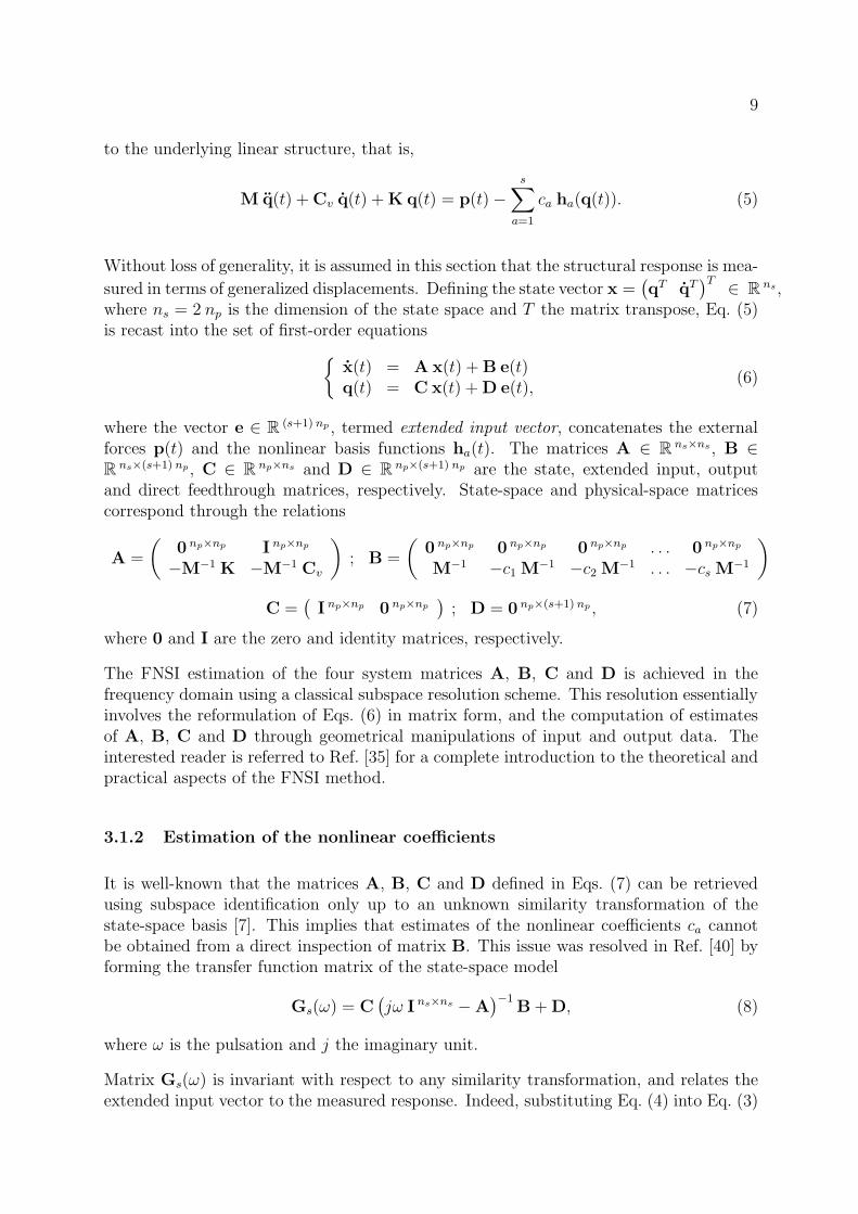
to the underlying linear structure, that is,
M q(t) +Cv q(t) +K q(t) = p(t)−s∑
a=1
ca ha(q(t)). (5)
Without loss of generality, it is assumed in this section that the structural response is mea-
sured in terms of generalized displacements. Defining the state vector x =(qT qT
)T∈ R
ns,where ns = 2 np is the dimension of the state space and T the matrix transpose, Eq. (5)is recast into the set of first-order equations
{x(t) = A x(t) +B e(t)q(t) = C x(t) +D e(t),
(6)
where the vector e ∈ R(s+1) np , termed extended input vector, concatenates the external
forces p(t) and the nonlinear basis functions ha(t). The matrices A ∈ Rns×ns, B ∈
Rns×(s+1) np, C ∈ R
np×ns and D ∈ Rnp×(s+1) np are the state, extended input, output
and direct feedthrough matrices, respectively. State-space and physical-space matricescorrespond through the relations
A =
(0 np×np I np×np
−M−1 K −M−1 Cv
); B =
(0 np×np 0 np×np 0 np×np . . . 0 np×np
M−1−c1 M
−1−c2 M
−1 . . . −cs M−1
)
C =(I np×np 0 np×np
); D = 0 np×(s+1) np , (7)
where 0 and I are the zero and identity matrices, respectively.
The FNSI estimation of the four system matrices A, B, C and D is achieved in thefrequency domain using a classical subspace resolution scheme. This resolution essentiallyinvolves the reformulation of Eqs. (6) in matrix form, and the computation of estimatesof A, B, C and D through geometrical manipulations of input and output data. Theinterested reader is referred to Ref. [35] for a complete introduction to the theoretical andpractical aspects of the FNSI method.
3.1.2 Estimation of the nonlinear coefficients
It is well-known that the matrices A, B, C and D defined in Eqs. (7) can be retrievedusing subspace identification only up to an unknown similarity transformation of thestate-space basis [7]. This implies that estimates of the nonlinear coefficients ca cannotbe obtained from a direct inspection of matrix B. This issue was resolved in Ref. [40] byforming the transfer function matrix of the state-space model
Gs(ω) = C(jω I ns×ns
−A)−1
B+D, (8)
where ω is the pulsation and j the imaginary unit.
Matrix Gs(ω) is invariant with respect to any similarity transformation, and relates theextended input vector to the measured response. Indeed, substituting Eq. (4) into Eq. (3)

10
and moving to the frequency domain yields
G−1(ω)Q(ω) +s∑
a=1
ca Ha(ω) = P(ω), (9)
where G(ω) = (−ω2 M+ j ω Cv +K)−1
is the transfer function matrix of the underlyinglinear system, and where Q(ω), Ha(ω) and P(ω) are the continuous Fourier transformsof q(t), ha(t) and p(t), respectively. The concatenation of P(ω) and Ha(ω) into theextended input spectrum E(ω) finally gives
Q(ω) = G(ω)[I np×np −c1 I
np×np . . . −cs Inp×np
]E(ω) = Gs(ω)E(ω). (10)
The nonlinear coefficients ca, together with the frequency response functions (FRFs) inG(ω), can be directly extracted from Eq. (10), given the transfer function matrix Gs(ω)estimated from Eq. (8).
3.2 Computation of NNMs in modal space
The calculation of NNMs is not realized in this work in state space but in modal space inorder to be compatible with the computational framework of Ref [25]. For that purpose,Eq. (1) is recast into
q(t) +K q(t) +
s∑
a=1
ca ΦT ha(q(t)) = 0, (11)
where q(t) = Φ−1q(t) is the vector of linear modal coordinates. Matrix Φ containsthe mode shapes φ(i) scaled to unit modal mass, i.e. M = ΦT M Φ = I np×np andK = ΦT KΦ = diag
(ω2i,0
).
To simulate Eq. (11), the knowledge of the undamped frequencies ωi,0, nonlinear coef-ficients ca, scaled mode shapes φ(i) and basis functions ha is required. The nonlinearcoefficients and basis functions are known from Section 3.1. The undamped frequenciesωi,0 are the absolute values of the complex eigenvalues λi of matrix A estimated usingFNSI in the previous section, that is,
Aψ(i) = λi ψ(i), i = 1, ..., ns. (12)
The state-space mode shapes ψ(i) are converted into the corresponding modes φ(i) inphysical space utilizing the output matrix C as
φ(i) = Cψ(i). (13)
Each mode shape vector φ(i) is then scaled using the residue R(i)kk of the driving point
FRF Gkk(ω) of the underlying linear system formulated as
Gkk(ω) =
np∑
i=1
R(i)kk
j ω − λi
+R
(i)∗
kk
j ω − λ∗
i
, (14)

11
where k is the location of the excited DOF, and where a star denotes the complex conjugateoperation. Eq. (14) is an overdetermined algebraic system of equations with np unknownsand as many equations as the number of processed frequency lines. The i-th scaled modeshape vector at the driving point φ
(i)k is finally obtained by enforcing a unit modal mass,
i.e.
R(i)kk =
φ(i)k φ
(i)k
2 j ωi,0, (15)
while the other components of the mode shape vector are scaled accordingly. This modescaling is rigorously valid in the case of linear proportional damping [41], which implies a
real-valued mode shape at the driving point φ(i)k . In general, experimental mode shapes
are however complex-valued. They can be enforced to be real by rotating each modein the complex plane by an angle equal to the mean of the phase angles of the modecomponents, and subsequently neglecting the imaginary parts of the rotated components.
The algorithm described in Ref. [25] can now be applied to seek NNMs, given that allquantities in Eq. (11) are known. To obtain the family of periodic solutions that de-scribe the considered NNM, shooting is combined with a pseudo-arclength continuationtechnique. Starting from a known periodic solution, continuation proceeds in two steps,namely a prediction and a correction, as illustrated in Fig. 4. In the prediction step, aguess of the next periodic solution along the NNM branch is generated in the direction ofthe tangent vector to the branch at the current solution. Next, the prediction is correctedusing a shooting procedure, forcing the variations of the period and the initial conditionsto be orthogonal to the prediction direction.
Frequency
Energy
b
Currentsolution
Tangentialprediction
bNext
solutionOrthogonalcorrection
Figure 4: Computation of a family of periodic solutions using a pseudo-arclength contin-uation scheme including prediction and correction steps.
12
4 Numerical demonstration using a cantilever beam
possessing a hardening-softening nonlinearity
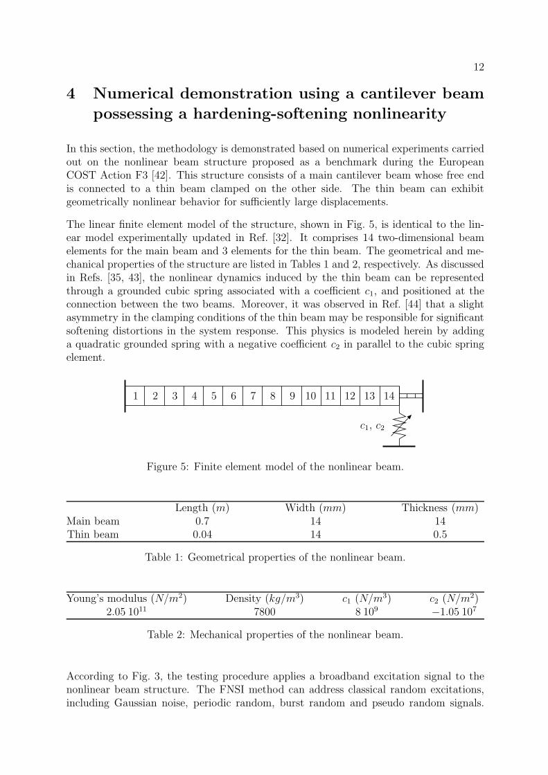
In this section, the methodology is demonstrated based on numerical experiments carriedout on the nonlinear beam structure proposed as a benchmark during the EuropeanCOST Action F3 [42]. This structure consists of a main cantilever beam whose free endis connected to a thin beam clamped on the other side. The thin beam can exhibitgeometrically nonlinear behavior for sufficiently large displacements.
The linear finite element model of the structure, shown in Fig. 5, is identical to the lin-ear model experimentally updated in Ref. [32]. It comprises 14 two-dimensional beamelements for the main beam and 3 elements for the thin beam. The geometrical and me-chanical properties of the structure are listed in Tables 1 and 2, respectively. As discussedin Refs. [35, 43], the nonlinear dynamics induced by the thin beam can be representedthrough a grounded cubic spring associated with a coefficient c1, and positioned at theconnection between the two beams. Moreover, it was observed in Ref. [44] that a slightasymmetry in the clamping conditions of the thin beam may be responsible for significantsoftening distortions in the system response. This physics is modeled herein by addinga quadratic grounded spring with a negative coefficient c2 in parallel to the cubic springelement.
1 2 3 4 5 6 7 8 9 10 11 12 13 14
c1, c2
Figure 5: Finite element model of the nonlinear beam.
Length (m) Width (mm) Thickness (mm)Main beam 0.7 14 14Thin beam 0.04 14 0.5
Table 1: Geometrical properties of the nonlinear beam.
Young’s modulus (N/m2) Density (kg/m3) c1 (N/m3) c2 (N/m2)2.05 1011 7800 8 109 −1.05 107
Table 2: Mechanical properties of the nonlinear beam.
According to Fig. 3, the testing procedure applies a broadband excitation signal to thenonlinear beam structure. The FNSI method can address classical random excitations,including Gaussian noise, periodic random, burst random and pseudo random signals.
13
Impulsive excitations also fall within the scope of the method, but they involve window-ing to avoid leakage and generally lead to low signal-to-noise ratios (SNRs). Swept-sineexcitations are not applicable because of the inability of the FNSI method to handle non-stationary signals, i.e. signals with time-varying frequency content [35]. One opts hereinfor pseudo random signals, also known as random phase multisine signals. A randomphase multisine is a periodic random signal with a user-controlled amplitude spectrum,and a random phase spectrum drawn from a uniform distribution. If an integer number ofperiods is measured, the amplitude spectrum is perfectly realized, unlike Gaussian noise.One of the other main advantages of a multisine is that its periodic nature can be utilizedto separate transient from steady-state oscillations in response time histories. This, inturn, eliminates the systematic errors due to leakage in the identification. Periodicity alsoallows the estimation of the covariance matrix of the noise perturbations affecting thesystem outputs.
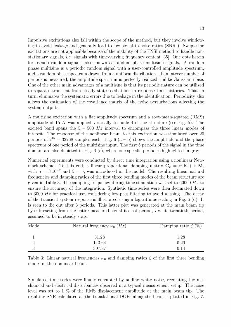
A multisine excitation with a flat amplitude spectrum and a root-mean-squared (RMS)amplitude of 15 N was applied vertically to node 4 of the structure (see Fig. 5). Theexcited band spans the 5 – 500 Hz interval to encompass the three linear modes ofinterest. The response of the nonlinear beam to this excitation was simulated over 20periods of 215 = 32768 samples each. Fig. 6 (a – b) shows the amplitude and the phasespectrum of one period of the multisine input. The first 5 periods of the signal in the timedomain are also depicted in Fig. 6 (c), where one specific period is highlighted in gray.
Numerical experiments were conducted by direct time integration using a nonlinear New-mark scheme. To this end, a linear proportional damping matrix Cv = α K + β M,with α = 3 10−7 and β = 5, was introduced in the model. The resulting linear naturalfrequencies and damping ratios of the first three bending modes of the beam structure aregiven in Table 3. The sampling frequency during time simulation was set to 60000 Hz toensure the accuracy of the integration. Synthetic time series were then decimated downto 3000 Hz for practical use, considering low-pass filtering to avoid aliasing. The decayof the transient system response is illustrated using a logarithmic scaling in Fig. 6 (d). Itis seen to die out after 3 periods. This latter plot was generated at the main beam tipby subtracting from the entire measured signal its last period, i.e. its twentieth period,assumed to be in steady state.
Mode Natural frequency ω0 (Hz) Damping ratio ζ (%)
1 31.28 1.282 143.64 0.293 397.87 0.14
Table 3: Linear natural frequencies ω0 and damping ratios ζ of the first three bendingmodes of the nonlinear beam.
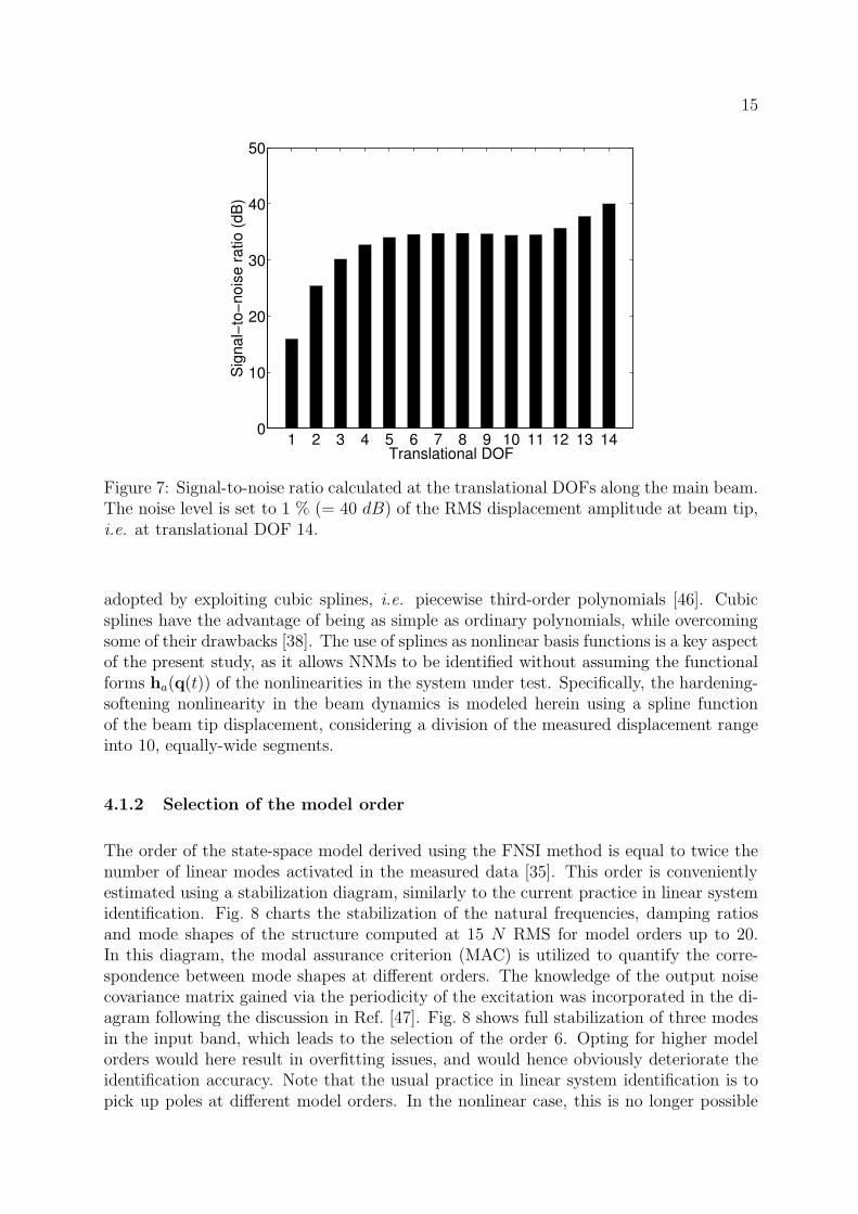
Simulated time series were finally corrupted by adding white noise, recreating the me-chanical and electrical disturbances observed in a typical measurement setup. The noiselevel was set to 1 % of the RMS displacement amplitude at the main beam tip. Theresulting SNR calculated at the translational DOFs along the beam is plotted in Fig. 7.

14
0 500 1000 1500−350
−250
−150
−50
50
Frequency (Hz)
Am
plit
ud
e (
dB
)
(a)
0 500 1000 1500−4
−2
0
2
4
Frequency (Hz)
Ph
ase
(ra
d)
(b)
0 1 2 3 4 5−80
−40
0
40
80
Period
Fo
rce
(N
)
(c)
0 1 2 3 4 5−300
−250
−200
−150
−100
−50
Period
Tra
nsie
nt
resp
on
se
(d
B)
(d)
Figure 6: Random phase multisine excitation signal. (a – b) Amplitude and phase spec-trum of a single period; (c) first 5 periods in the time domain with one specific periodhighlighted in gray; (d) decay of the transient system response illustrated using a loga-rithmic scaling at the main beam tip over 5 periods.
It is found that imposing 1 % noise at the tip, i.e. a SNR of 40 dB at DOF 14 in Fig. 7,results in more severe noise conditions at all other sensors. In particular, at mid-span,the SNR is around 34 dB, while it is lower than 30 dB close to the left clamping.
4.1 Identification using the FNSI method
4.1.1 Selection of the nonlinear basis functions
The application of the FNSI method to measured data requires the selection of appropriatebasis functions ha(q(t)) to describe the nonlinearity in the system. This task, referredto as the characterization of nonlinearity, is in general challenging because of the varioussources of nonlinear behavior that may exist in engineering structures, and the plethoraof dynamic phenomena they may cause [45]. In this work, a gray-box methodology is
15
1 2 3 4 5 6 7 8 9 10 11 12 13 140
10
20
30
40
50
Translational DOF
Sig
nal−
to−
nois
e r
atio (
dB
)
Figure 7: Signal-to-noise ratio calculated at the translational DOFs along the main beam.The noise level is set to 1 % (= 40 dB) of the RMS displacement amplitude at beam tip,i.e. at translational DOF 14.
adopted by exploiting cubic splines, i.e. piecewise third-order polynomials [46]. Cubicsplines have the advantage of being as simple as ordinary polynomials, while overcomingsome of their drawbacks [38]. The use of splines as nonlinear basis functions is a key aspectof the present study, as it allows NNMs to be identified without assuming the functionalforms ha(q(t)) of the nonlinearities in the system under test. Specifically, the hardening-softening nonlinearity in the beam dynamics is modeled herein using a spline functionof the beam tip displacement, considering a division of the measured displacement rangeinto 10, equally-wide segments.
4.1.2 Selection of the model order
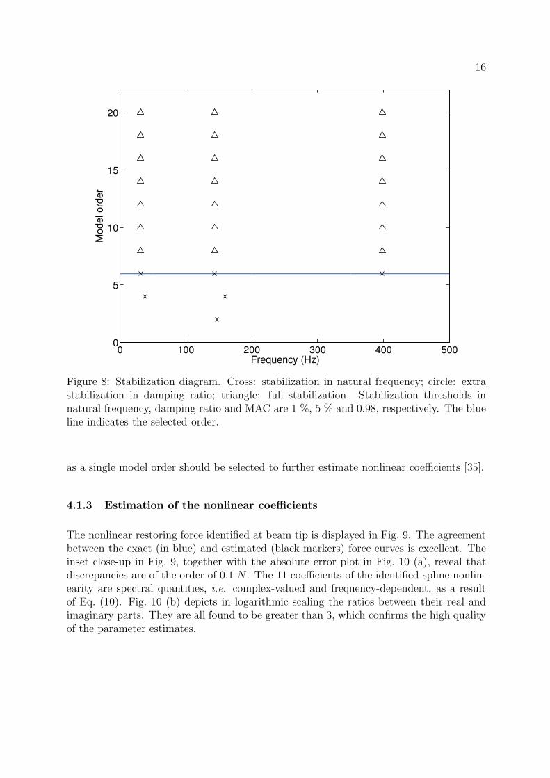
The order of the state-space model derived using the FNSI method is equal to twice thenumber of linear modes activated in the measured data [35]. This order is convenientlyestimated using a stabilization diagram, similarly to the current practice in linear systemidentification. Fig. 8 charts the stabilization of the natural frequencies, damping ratiosand mode shapes of the structure computed at 15 N RMS for model orders up to 20.In this diagram, the modal assurance criterion (MAC) is utilized to quantify the corre-spondence between mode shapes at different orders. The knowledge of the output noisecovariance matrix gained via the periodicity of the excitation was incorporated in the di-agram following the discussion in Ref. [47]. Fig. 8 shows full stabilization of three modesin the input band, which leads to the selection of the order 6. Opting for higher modelorders would here result in overfitting issues, and would hence obviously deteriorate theidentification accuracy. Note that the usual practice in linear system identification is topick up poles at different model orders. In the nonlinear case, this is no longer possible
16
0 100 200 300 400 5000
5
10
15
20
Frequency (Hz)
Model ord
er
Figure 8: Stabilization diagram. Cross: stabilization in natural frequency; circle: extrastabilization in damping ratio; triangle: full stabilization. Stabilization thresholds innatural frequency, damping ratio and MAC are 1 %, 5 % and 0.98, respectively. The blueline indicates the selected order.
as a single model order should be selected to further estimate nonlinear coefficients [35].
4.1.3 Estimation of the nonlinear coefficients
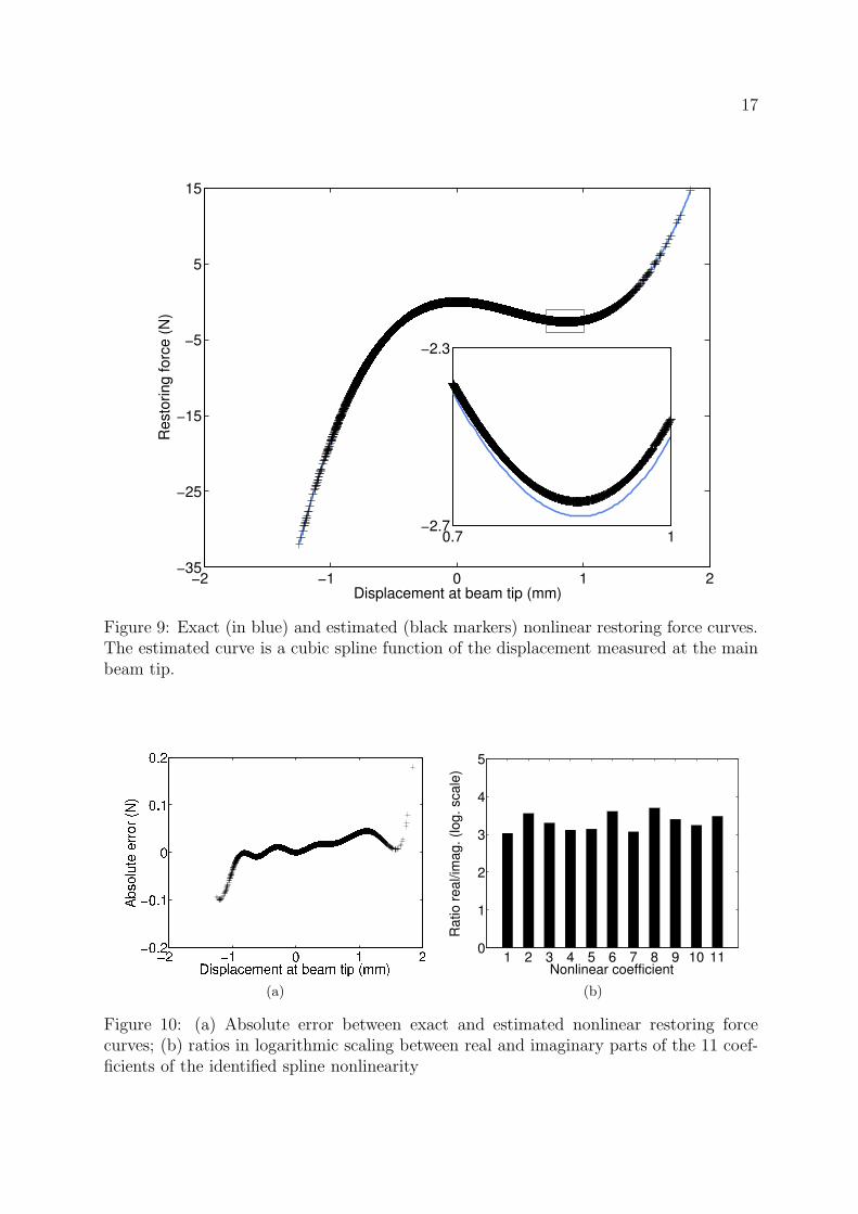
The nonlinear restoring force identified at beam tip is displayed in Fig. 9. The agreementbetween the exact (in blue) and estimated (black markers) force curves is excellent. Theinset close-up in Fig. 9, together with the absolute error plot in Fig. 10 (a), reveal thatdiscrepancies are of the order of 0.1 N . The 11 coefficients of the identified spline nonlin-earity are spectral quantities, i.e. complex-valued and frequency-dependent, as a resultof Eq. (10). Fig. 10 (b) depicts in logarithmic scaling the ratios between their real andimaginary parts. They are all found to be greater than 3, which confirms the high qualityof the parameter estimates.
17
−2 −1 0 1 2−35
−25
−15
−5
5
15
Displacement at beam tip (mm)
Resto
ring forc
e (
N)
0.7 1−2.7
−2.3
Figure 9: Exact (in blue) and estimated (black markers) nonlinear restoring force curves.The estimated curve is a cubic spline function of the displacement measured at the mainbeam tip.
(a)
1 2 3 4 5 6 7 8 9 10 110
1
2
3
4
5
Ratio r
eal/im
ag. (log. scale
)
Nonlinear coefficient
(b)
Figure 10: (a) Absolute error between exact and estimated nonlinear restoring forcecurves; (b) ratios in logarithmic scaling between real and imaginary parts of the 11 coef-ficients of the identified spline nonlinearity
18
4.2 Computation of the first two NNMs using continuation
In this section, the first two NNMs of the beam structure are computed by applying thealgorithm of Section 3.2 to Eqs. (11) populated with the nonlinear and linear parametersestimated using FNSI. Nonlinear parameter estimates were discussed in the previous sec-tion. Table 4 lists the relative errors on the linear natural frequencies and damping ratiostogether with the diagonal MAC values. The results in this table demonstrate the abilityof the FNSI method to recover accurately the modal properties of the underlying linearstructure from nonlinear data. Note that the third mode will not be further analyzedherein as it involves virtually no nonlinear distortions.
Mode Error on ω0 (%) Error on ζ (%) MAC
1 0.0008 -0.0758 1.002 -0.0015 0.0709 1.003 -0.0144 -0.1015 1.00
Table 4: Relative errors on the estimated natural frequencies and damping ratios (in %)and diagonal MAC values of the first three modes of the beam computed at order 6.
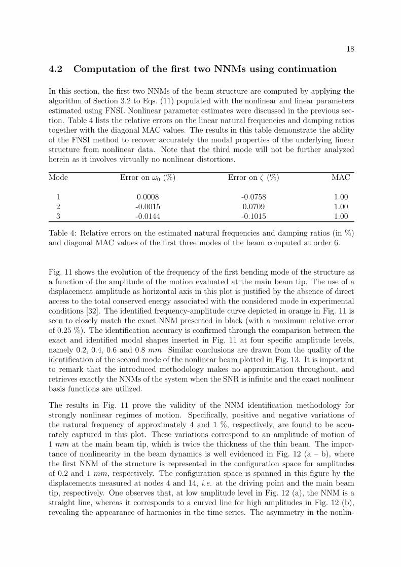
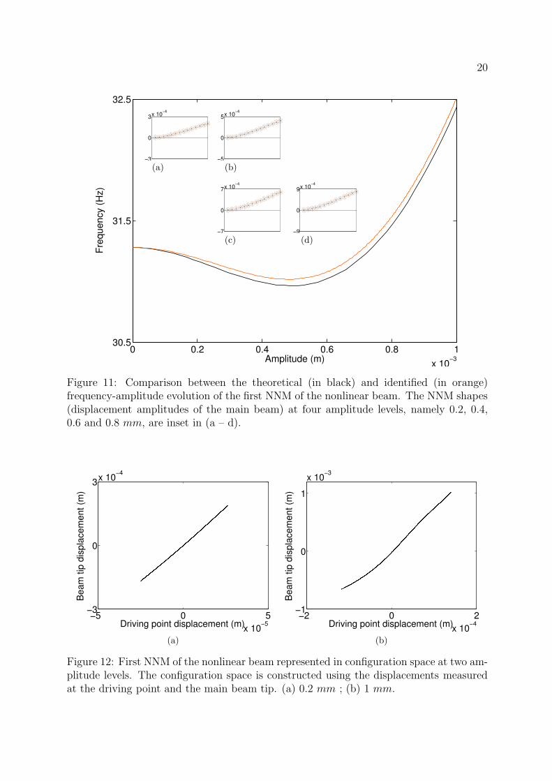
Fig. 11 shows the evolution of the frequency of the first bending mode of the structure asa function of the amplitude of the motion evaluated at the main beam tip. The use of adisplacement amplitude as horizontal axis in this plot is justified by the absence of directaccess to the total conserved energy associated with the considered mode in experimentalconditions [32]. The identified frequency-amplitude curve depicted in orange in Fig. 11 isseen to closely match the exact NNM presented in black (with a maximum relative errorof 0.25 %). The identification accuracy is confirmed through the comparison between theexact and identified modal shapes inserted in Fig. 11 at four specific amplitude levels,namely 0.2, 0.4, 0.6 and 0.8 mm. Similar conclusions are drawn from the quality of theidentification of the second mode of the nonlinear beam plotted in Fig. 13. It is importantto remark that the introduced methodology makes no approximation throughout, andretrieves exactly the NNMs of the system when the SNR is infinite and the exact nonlinearbasis functions are utilized.
The results in Fig. 11 prove the validity of the NNM identification methodology forstrongly nonlinear regimes of motion. Specifically, positive and negative variations ofthe natural frequency of approximately 4 and 1 %, respectively, are found to be accu-rately captured in this plot. These variations correspond to an amplitude of motion of1 mm at the main beam tip, which is twice the thickness of the thin beam. The impor-tance of nonlinearity in the beam dynamics is well evidenced in Fig. 12 (a – b), wherethe first NNM of the structure is represented in the configuration space for amplitudesof 0.2 and 1 mm, respectively. The configuration space is spanned in this figure by thedisplacements measured at nodes 4 and 14, i.e. at the driving point and the main beamtip, respectively. One observes that, at low amplitude level in Fig. 12 (a), the NNM is astraight line, whereas it corresponds to a curved line for high amplitudes in Fig. 12 (b),revealing the appearance of harmonics in the time series. The asymmetry in the nonlin-

19
ear restoring force in the system is also clearly visible. A similar analysis is achieved inFig. 14 (a – b) for the second NNM of the beam. These two graphs show that, owingto the displacement nature of the involved nonlinearity, higher-frequency modes are lessimpacted by harmonic distortions, and translate into straight lines in configuration spaceeven for large amplitudes of motion. In this study, the amplitude interval over whichthe continuation was performed was merely selected by observing that the maximum am-plitude of displacement recorded in Section 4.1 at the main beam tip under multisineforcing was of the order of 1 mm. However, a rigorous evaluation of the validity rangesof identified frequency-amplitude plots deserves more investigation.
5 Comparison with NNMs identified using nonlinear
phase resonance
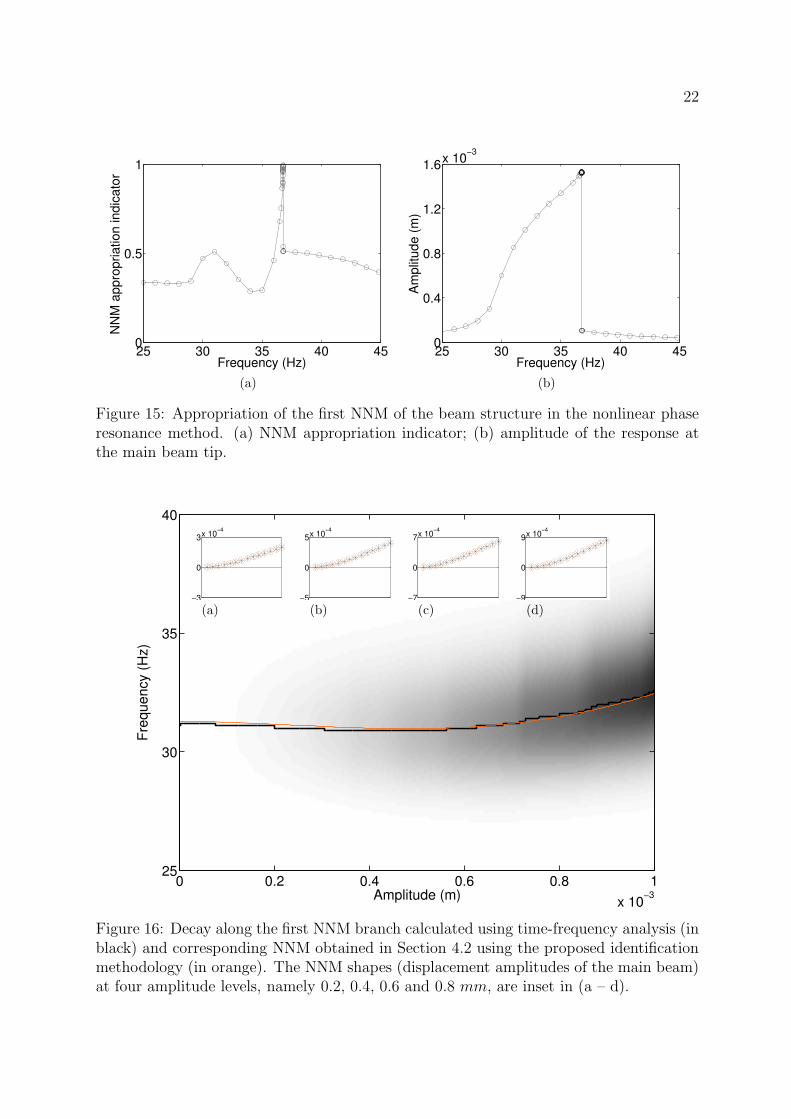
As depicted in Fig. 2, the first step of the nonlinear phase resonance testing procedureis the isolation of the NNM of interest. To this end, a 3 N sine signal is applied tonode 4 of the structure. The frequency of this stepped-sine excitation is tuned until theforce appropriation indicator derived from the generalized phase lag quadrature criterionis equal to 1 [32]. Fig. 15 (a) shows that NNM appropriation is achieved at 36.8 Hz forthe first beam mode. The corresponding amplitude of the forced response at beam tip inFig. 15 (b) depicts the distorted frequency response of the mode and the sudden jumpoccurring as soon as resonance is passed.
When the considered NNM is appropriated, the second step of the procedure turns offthe excitation in order to observe the free decay of the system along the NNM branch. Atime-frequency analysis of the decaying time response is then carried out to extract thefrequency-energy dependence of the mode. This is achieved in Fig. 16 where the wavelettransform of the displacement measured at beam tip is represented. The ridge of thewavelet, i.e. the locus of maximum amplitude with respect to frequency, is presented as ablack line, and is seen to closely coincide with the NNM identified in the previous sectionand plotted in orange. The comparable accuracy of the phase separation and phaseresonance approaches is confirmed by the modal shapes superposed at four amplitudelevels in Fig. 16. The results in this figure, together with the analysis of the second NNMappropriation in Figs. 17 and 18, clearly confirm the accuracy of this new nonlinear phaseseparation technique. In summary, Table 5 lists the strengths and limitations of the twomethodologies.
20
0 0.2 0.4 0.6 0.8 1
x 10−3
30.5
31.5
32.5
Amplitude (m)
Fre
qu
en
cy (
Hz)
−3
0
3x 10
−4
−5
0
5x 10
−4
−7
0
7x 10
−4
−9
0
9x 10
−4
(a) (b)
(c) (d)
Figure 11: Comparison between the theoretical (in black) and identified (in orange)frequency-amplitude evolution of the first NNM of the nonlinear beam. The NNM shapes(displacement amplitudes of the main beam) at four amplitude levels, namely 0.2, 0.4,0.6 and 0.8 mm, are inset in (a – d).
−5 0 5
x 10−5
−3
0
3x 10
−4
Driving point displacement (m)
Be
am
tip
dis
pla
ce
me
nt
(m)
(a)
−2 0 2
x 10−4
−1
0
1
x 10−3
Driving point displacement (m)
Be
am
tip
dis
pla
ce
me
nt
(m)
(b)
Figure 12: First NNM of the nonlinear beam represented in configuration space at two am-plitude levels. The configuration space is constructed using the displacements measuredat the driving point and the main beam tip. (a) 0.2 mm ; (b) 1 mm.

21
0 0.2 0.4 0.6 0.8 1
x 10−3
143.4
143.6
143.8
144
Amplitude (m)
Fre
qu
en
cy (
Hz)
−3
0
3x 10
−4
−5
0
5x 10
−4
−7
0
7x 10
−4
−9
0
9x 10
−4
(a) (b)
(c) (d)
Figure 13: Comparison between the theoretical (in black) and identified (in orange)frequency-amplitude evolution of the second NNM of the nonlinear beam. The NNMshapes (displacement amplitudes of the main beam) at four amplitude levels, namely 0.2,0.4, 0.6 and 0.8 mm, are inset in (a – d).
−2 0 2
x 10−4
−3
0
3x 10
−4
Driving point displacement (m)
Be
am
tip
dis
pla
ce
me
nt
(m)
(a)
−6 0 6
x 10−4
−1
0
1
x 10−3
Driving point displacement (m)
Be
am
tip
dis
pla
ce
me
nt
(m)
(b)
Figure 14: Second NNM of the nonlinear beam represented in configuration space attwo amplitude levels. The configuration space is constructed using the displacementsmeasured at the driving point and the main beam tip. (a) 0.2 mm ; (b) 1 mm.
22
25 30 35 40 450
0.5
1
Frequency (Hz)
NN
M a
ppro
priation indic
ato
r
(a)
25 30 35 40 450
0.4
0.8
1.2
1.6x 10
−3
Frequency (Hz)
Am
plit
ude (
m)
(b)
Figure 15: Appropriation of the first NNM of the beam structure in the nonlinear phaseresonance method. (a) NNM appropriation indicator; (b) amplitude of the response atthe main beam tip.
Amplitude (m)
Fre
quency (
Hz)
0 0.2 0.4 0.6 0.8 1
x 10−3
25
30
35
40
−3
0
3x 10
−4
−5
0
5x 10
−4
−7
0
7x 10
−4
−9
0
9x 10
−4
(a) (b) (c) (d)
Figure 16: Decay along the first NNM branch calculated using time-frequency analysis (inblack) and corresponding NNM obtained in Section 4.2 using the proposed identificationmethodology (in orange). The NNM shapes (displacement amplitudes of the main beam)at four amplitude levels, namely 0.2, 0.4, 0.6 and 0.8 mm, are inset in (a – d).

23
142 144 146 1480
0.5
1
Frequency (Hz)
NN
M a
ppro
priation indic
ato
r
(a)
142 144 146 1480
0.4
0.8
1.2
1.6x 10
−3
Frequency (Hz)
Am
plit
ude (
m)
(b)
Figure 17: Appropriation of the second NNM of the beam structure in the nonlinear phaseresonance method. (a) NNM appropriation indicator; (b) amplitude of the response atthe main beam tip.
Amplitude (m)
Fre
quency (
Hz)
0 0.2 0.4 0.6 0.8 1
x 10−3
135
140
145
150
−3
0
3x 10
−4
−5
0
5x 10
−4
−7
0
7x 10
−4
−9
0
9x 10
−4
(a) (b) (c) (d)
Figure 18: Decay along the second NNM branch calculated using time-frequency analysis(in black) and corresponding NNM obtained in Section 4.2 using the proposed identifica-tion methodology (in orange). The NNM shapes (displacement amplitudes of the mainbeam) at four amplitude levels, namely 0.2, 0.4, 0.6 and 0.8 mm, are inset in (a – d).

24
Nonlinear phase Nonlinear phaseseparation method resonance method
Fast Time-consuming(multiple NNMs (one NNM at a time)simultaneously)
Need of an Model-freeexperimental model
Classical random Harmonicexcitation can be utilized forcing must be tuned
Nonlinear components must Shaker mustbe instrumented on both sides be turned off
Nonlinearity characterization Limited information neededis required about the nonlinearities
Table 5: Comparison of the strengths and limitations of the two methodologies.
6 Conclusion
The present paper extracted the nonlinear normal modes (NNMs) of vibrating systemsfrom measurements collected under broadband forcing. A key feature of the proposedmethod is that it makes no assumption as to the strength of the nonlinearities and themodal couplings. Together with the previously-developed NNM identification methodbased on stepped-sine forcing, they provide a rigorous generalization of modal testing tononlinear systems.
The accuracy of the method was demonstrated numerically considering important noiseperturbations and no prior knowledge about the nonlinearities in the system, which pavesthe way for a future experimental validation of the method. In its current state, themethod can only handle stiffness nonlinearities. Further research will address this limi-tation by computing damped NNMs from the experimentally-derived state-space modelusing, e.g., the computational technique proposed in Ref. [27].
Acknowledgments
The author J.P. Noel is a Postdoctoral Researcher of the Fonds de la Recherche Scien-tifique – FNRS which is gratefully acknowledged. The author L. Renson is a Marie-Curie

25
COFUND Postdoctoral Fellow of the University of Liege, co-funded by the EuropeanUnion. The authors C. Grappasonni and G. Kerschen would finally like to acknowledgethe financial support of the European Union (ERC Starting Grant NoVib 307265).
References
[1] D.J. Ewins. A future for experimental structural dynamics. In Proceedings of theInternational Conference on Noise and Vibration Engineering (ISMA), Leuven, Bel-gium, 2006.
[2] B. Peeters, H. Climent, R. de Diego, J. de Alba, J.R. Ahlquist, J.M. Carreno, W. Hen-dricx, A. Rega, G. Garcia, J. Deweer, and J. Debille. Modern solutions for GroundVibration Testing of large aircraft. In Proceedings of the 26th International ModalAnalysis Conference (IMAC), Orlando, FL, USA, 2008.
[3] D. Goge, M. Boswald, U. Fullekrug, and P. Lubrina. Ground vibration testing oflarge aircraft: State of the art and future perspectives. In Proceedings of the 25thInternational Modal Analysis Conference (IMAC), Orlando, FL, USA, 2007.
[4] A. Grillenbeck and S. Dillinger. Reliability of experimental modal data determined onlarge spaceflight structures. In Proceedings of the 29th International Modal AnalysisConference (IMAC), Jacksonville, FL, USA, 2011.
[5] J.R. Wright, J.E. Cooper, and M.J. Desforges. Normal-mode force appropriation -theory and application. Mechanical Systems and Signal Processing, 13:217–240, 1999.
[6] B. Peeters, H. Van der Auweraer, P. Guillaume, and J. Leuridan. The PolyMAXfrequency-domain method: A new standard for modal parameter estimation? Shockand Vibration, 11(3-4):395–409, 2004.
[7] P. Van Overschee and B. De Moor. Subspace Identification for Linear Systems:Theory, Implementation and Applications. Kluwer Academic Publishers, Dordrecht,The Netherlands, 1996.
[8] P. Atkins, J.R. Wright, and K. Worden. An extension of force appropriation to theidentification of non-linear multi-degree of freedom systems. Journal of Sound andVibration, 237:23–43, 2000.
[9] M.F. Platten, J.R.Wright, G. Dimitriadis, and J.E. Cooper. Identification of multi-degree of freedom non-linear systems using an extended modal space model. Me-chanical Systems and Signal Processing, 23:8–29, 2009.
[10] C.W. Poon and C.C. Chang. Identification of nonlinear elastic structures usingempirical mode decomposition and nonlinear normal modes. Smart Structures andSystems, 3:423–437, 2007.

26
[11] A.F. Vakakis, L.A. Bergman, D.M. McFarland, Y.S. Lee, and M. Kurt. Currentefforts towards a non-linear system identification methodology of broad applicability.Proceedings of the Institution of Mechanical Engineers, Part C: Journal of MechanicalEngineering Science, 225:2497–2515, 2011.
[12] M. Eriten, M. Kurt, G. Luo, A.F. Vakakis, D.M. McFarland, and L.A. Bergman.Nonlinear system identification of frictional effects in a beam with bolted connection.Mechanical Systems and Signal Processing, 39:245–264, 2013.
[13] P.F. Pai. Time-frequency characterization of nonlinear normal modes and challengesin nonlinearity identification of dynamical systems. Mechanical Systems and SignalProcessing, 25:2358–2374, 2011.
[14] K. Worden and P.L. Green. A machine learning approach to nonlinear modal anal-ysis. In Proceedings of the 32nd International Modal Analysis Conference (IMAC),Orlando, FL, USA, 2014.
[15] C. Gibert. Fitting measured frequency response functions using non-linear modes.Mechanical Systems and Signal Processing, 17:211–218, 2003.
[16] Y.H. Chong and M. Imregun. Development and application of a nonlinear modalanalysis technique for MDOF systems. Journal of Vibration and Control, 7:167–179,2001.
[17] R.M. Rosenberg. The normal modes of nonlinear n-degree-of-freedom systems. Jour-nal of Applied Mechanics, 29:7–14, 1962.
[18] R.M. Rosenberg. On nonlinear vibrations of systems with many degrees of freedom.Advances in Applied Mechanics, 9:217–240, 1966.
[19] S.W. Shaw and C. Pierre. Normal modes for non-linear vibratory systems. Journalof Sound and Vibration, 164(1):85–124, 1993.
[20] A.F. Vakakis, L.I. Manevitch, Y.V. Mlkhlin, V.N. Pilipchuk, and A.A. Zevin. NormalModes and Localization in Nonlinear Systems. John Wiley & Sons, New-York, NY,USA, 1996.
[21] W. Lacarbonara and R. Camillacci. Nonlinear normal modes of structural systems viaasymptotic approach. International Journal of Solids and Structures, 41:5565–5594,2004.
[22] C. Touze and M. Amabili. Nonlinear normal modes for damped geometrically non-linear systems: Application to reduced-order modelling of harmonically forced struc-tures. Journal of Sound and Vibration, 298:958–981, 2006.
[23] G. Kerschen, M. Peeters, J.C. Golinval, and A.F. Vakakis. Nonlinear normal modes.Part I: A useful framework for the structural dynamicist. Mechanical Systems andSignal Processing, 23(1):170–194, 2009.

27
[24] R. Arquier, S. Bellizzi, R. Bouc, and B. Cochelin. Two methods for the computa-tion of nonlinear modes of vibrating systems at large amplitudes. Computers andStructures, 84:1565–1576, 2006.
[25] M. Peeters, R. Viguie, G. Serandour, G. Kerschen, and J.C. Golinval. Nonlinearnormal modes. Part II: Toward a practical computation using numerical continuationtechniques. Mechanical Systems and Signal Processing, 23(1):195–216, 2009.
[26] D. Laxalde and F. Thouverez. Complex non-linear modal analysis of mechanicalsystems: Application to turbomachinery bladings with friction interfaces. Journal ofSound and Vibration, 322:1009–1025, 2009.
[27] L. Renson, G. Deliege, and G. Kerschen. An effective finite-element-based method forthe computation of nonlinear normal modes of nonconservative systems. Meccanica,49(8):1901–1916, 2014.
[28] G. Kerschen, M. Peeters, J.C. Golinval, and C. Stephan. Nonlinear modal analysisof a full-scale aircraft. Journal of Aircraft, 50:1409–1419, 2013.
[29] L. Renson, J.P. Noel, and G. Kerschen. Complex dynamics of a nonlinearaerospace structure: Numerical continuation and normal modes. Nonlinear Dynam-ics, 79(2):1293–1309, 2014.
[30] M. Krack, L. Panning-von Scheidt, and J. Wallaschek. A method for nonlinearmodal analysis and synthesis: Application to harmonically forced and self-excitedmechanical systems. Journal of Sound and Vibration, 332(25):6798–6814, 2014.
[31] M. Peeters, G. Kerschen, and J.C. Golinval. Dynamic testing of nonlinear vibratingstructures using nonlinear normal modes. Journal of Sound and Vibration, 330:486–509, 2011.
[32] M. Peeters, G. Kerschen, and J.C. Golinval. Modal testing of nonlinear vibratingstructures based on nonlinear normal modes: Experimental demonstration. Mechan-ical Systems and Signal Processing, 25:1227–1247, 2011.
[33] J.L. Zapico-Valle, M. Garcia-Dieguez, and R. Alonso-Camblor. Nonlinear modalidentification of a steel frame. Engineering Structures, 56:246–259, 2013.
[34] D.A. Ehrhardt, R.B. Harris, and M.S. Allen. Numerical and experimental determi-nation of nonlinear normal modes of a circular perforated plate. In Proceedings of the32nd International Modal Analysis Conference (IMAC), Orlando, FL, USA, 2014.
[35] J.P. Noel and G. Kerschen. Frequency-domain subspace identification for nonlinearmechanical systems. Mechanical Systems and Signal Processing, 40:701–717, 2013.
[36] J.P. Noel, L. Renson, and G. Kerschen. Complex dynamics of a nonlinear aerospacestructure: Experimental identification and modal interactions. Journal of Sound andVibration, 333:2588–2607, 2014.
28
[37] J.P. Noel, S. Marchesiello, and G. Kerschen. Subspace-based identification of a non-linear spacecraft in the time and frequency domains. Mechanical Systems and SignalProcessing, 43:217–236, 2014.
[38] J.P. Noel, G. Kerschen, E. Foltete, and S. Cogan. Grey-box identification of a non-linear solar array structure using cubic splines. International Journal of Non-linearMechanics, accepted for publication, 2014.
[39] D.E. Adams and R.J. Allemang. A frequency domain method for estimating theparameters of a non-linear structural dynamic model through feedback. MechanicalSystems and Signal Processing, 14:637–656, 2000.
[40] S. Marchesiello and L. Garibaldi. A time domain approach for identifying nonlinearvibrating structures by subspace methods. Mechanical Systems and Signal Process-ing, 22:81–101, 2008.
[41] M. Geradin and D. Rixen. Mechanical Vibrations: Theory and Applications to Struc-tural Dynamics. John Wiley & Sons, Chichester, UK, 1997.
[42] F. Thouverez. Presentation of the ECL benchmark. Mechanical Systems and SignalProcessing, 17(1):195–202, 2003.
[43] G. Kerschen, V. Lenaerts, and J.C. Golinval. Identification of a continuous structurewith a geometrical non-linearity. Part I: Conditioned reverse path method. Journalof Sound and Vibration, 262:889–906, 2003.
[44] C. Grappasonni, J.P. Noel, and G. Kerschen. Subspace and nonlinear-normal-modes-based identification of a beam with softening-hardening behaviour. In Proceedingsof the 32nd International Modal Analysis Conference (IMAC), Orlando, FL, USA,2014.
[45] G. Kerschen, K. Worden, A.F. Vakakis, and J.C. Golinval. Past, present and futureof nonlinear system identification in structural dynamics. Mechanical Systems andSignal Processing, 20:505–592, 2006.
[46] C. De Boor. A Practical Guide to Splines. Springer-Verlag, New York, NY, 1978.
[47] T. McKelvey, H. Akcay, and L. Ljung. Subspace-based multivariable system iden-tification from frequency response data. IEEE Transactions on Automatic Control,41(7):960–979, 1996.