identification and control of mimo industrial processes : an integration approach · identification...

Identification and control of MIMO industrial processes : anintegration approachCitation for published version (APA):Zhu, Y. (1990). Identification and control of MIMO industrial processes : an integration approach. Eindhoven:Technische Universiteit Eindhoven. https://doi.org/10.6100/IR324744

DOI:10.6100/IR324744

Document status and date:Published: 01/01/1990

Document Version:Publisher’s PDF, also known as Version of Record (includes final page, issue and volume numbers)

Please check the document version of this publication:

• A submitted manuscript is the version of the article upon submission and before peer-review. There can beimportant differences between the submitted version and the official published version of record. Peopleinterested in the research are advised to contact the author for the final version of the publication, or visit theDOI to the publisher's website.• The final author version and the galley proof are versions of the publication after peer review.• The final published version features the final layout of the paper including the volume, issue and pagenumbers.Link to publication

General rightsCopyright and moral rights for the publications made accessible in the public portal are retained by the authors and/or other copyright ownersand it is a condition of accessing publications that users recognise and abide by the legal requirements associated with these rights.

• Users may download and print one copy of any publication from the public portal for the purpose of private study or research. • You may not further distribute the material or use it for any profit-making activity or commercial gain • You may freely distribute the URL identifying the publication in the public portal.

If the publication is distributed under the terms of Article 25fa of the Dutch Copyright Act, indicated by the “Taverne” license above, pleasefollow below link for the End User Agreement:www.tue.nl/taverne

Take down policyIf you believe that this document breaches copyright please contact us at:[email protected] details and we will investigate your claim.

Download date: 09. Mar. 2020

https://doi.org/10.6100/IR324744

https://doi.org/10.6100/IR324744

https://research.tue.nl/en/publications/identification-and-control-of-mimo-industrial-processes--an-integration-approach(b3d9c1ba-6ee9-46e0-be2c-d7aa05cebcf7).html

ldentification and Control of MIMO lndustrial processes: An lntegration Approach

m iJt Ëj tl iftJJ é91f m ttt 1r PÁ & 1± $ ~ :il I~ ttfï 1: é9 mm.

ZHU, Yu-Cai

To all the people

who have contributed, directly and indirectly, to this work

IDENTIFICATION AND CONTROL OF MIMO INDUSTRIAL PROCESSES:

AN INTEGRATION APPROACH

Proefschrift

ter verkrijging van de graad van doctor aan

de Technische Universiteit Eindhoven, op gezag van

de rector magnificus, prof. ir. M. Tels, voor een

commissie aangewezen door het college van dekanen

in het openbaar te verdedigen op

dinsdag 13 februari 1990 om 16.00 uur

door

ZHU, Yu-Cai

geboren te Bole, Xinjiang, China

Dit proefschrift is goedgekeurd door

de promotor Prof. dr. ir. P. Eykhoff

en

de copromotor Dr. ir. A.A.H. Damen

CJP-GEGEVENS KONINKLIJKE BIBLIOTHEEK, DEN HAAG

ZHU, Yu-Cai

Identification and control of MIMO industrial processes:

an integration approach I ZHU, Yu-Cai. -[S.l.:s .. n.].

Fig., tab.

Proefschrift Eindhoven. -Met lit. opg., reg.

ISBN 90-9003261-4

SISO 656.2 UDC 519.71.001.3(043.3) NUGI 832

Trefw.: systeemidentificatie; procesregeling.

CONTENTS

Summary

1 Introduetion

1.1 An Integration Approach, What and Why?

1.2 The philosophy of Identification

1.3 Defining and Analyzing the Problems

1.4 Scope of This Thesis

2 Asymptotic Properties of Black-Box MIMO Transfer Function

Estimates

2.1 Introduetion

2.2 Speetral Analysis Methad

2.3 Prediction Error Methad

2.3.1 Black-Box Models and Shift Property

2.3.2 Asymptotic Properties of Prediction Error Models

2.4 Conclusions

Appendix 2.A Proof of Theorem 2.2.1

Appendix 2.B Kronecker Products

Appendix 2.C Proof of Lemma 2.3.2

Appendix 2.D Proof of Lemma 2.3.3

3 ldentifying the Nomina! Model and the Error Bounds

3.1 Introduetion

3.2 Algorithms by Speetral Analysis

3.3 Algorithms by Prediction Error Method

3.3.1 Two Simple Model Structures

3.3.2 The Nomina! Model and the Upper Bound Matrix

3.4 Conclusions

4 Robust Stability of MIMO Linear Feedback Systems

4.1 Introduetion

4.2 Robust Stability Analysis

4.2.1 The Class of Perturbations

4.2.2 Robust Stability Criteria

I

IV

1

4

7

10

12

12

14

18

19

22

32

33

36

37

39

41

41

42

50

50

51

57

57

58 59

59

60

4.2.3 Comparing the Three Criteria 64 4.3 Robust Stability of Internal Model Control Scheme 66 4.4 A Procedure from Identification to Robust Control 68 4.5 Conclusions 71

s An Approach to Linking ldentification and Control 72

5.1 Introduetion 72

5.2 The Problem and Some Conventional Solutions 73 5.3 The New Scheme 76 5.4 Analysis of the New Scheme 78

5.4.1 Some Notes on Approximate Modelling 78 5.4.2 Accuracy Aspects of the Process Model and

System Model 84 5.4.3 The Optimality of the Two Loop System Structure 87

5.5 A Case Srudy 89 5.5.1 Results of ldentification 90

5.4.2 Results of Control 92 5.6 Condus i ons 99

6 An Industrial Application 101 6.1 Introduetion 101 6.2 Examining and Analyzing the Existing Control System 102 6.3 Input Design and Model Validation 105 6.4 Readjustment of the Feedback Filter 108 6.5 Conclusions 111

7 Conclusions 121

Relerences 123

Symbols and Abbreviations 128

Curriculum Vitae 131

II

rt~miR & iirt ~ lMI! ~~ ~ -szi)l)~ ~Ojt~~~tr ~; tt~ ~llfiJ & j~ iitt~ DJPJ rl ~ ~ À x') ~ lli il! fT iJ1J ,-, * I f't ~ i-1 m iR Èi ~ llf~ ffi ~ .g. ~ fiïj I! ~Ik :(± ~ ~~:I:I.'l:ii~J::~JiiZJij, .ZPJf~~S!iiJIJ" ~.g.":::. Ji!.llL~~ffJ~~ trilil m iRËi ~lli~ik m -t;t Y:. Ojtf4~ it :t 1lli:llM~ mt'* et~1~ 3t 4, ~;!}IJ &X<t ~·lil' i,lt; 5!- trilil, ~jij mi.RfP~lfill *ltH\~~ ~jj(fiïJ 1!111, liP~~ l'i.lt~i~it ~miR J'Ji~~~ ~ ~li:IJ, tEm~~~ iî J::ii "fl- ~1l* fiiJ I! l!("fl ~fll llii71Uf~. :l- * fiîJ e.z-&~~- -tt:'t ~~x1mi.RiJL~.~~J:!ll; ik ~J:!llx<tr mm mi.Rffl~~ ~il!rr.ff..Mt~lli~ l'tJt~ 7t :tlfÉJ ~it & ~,aY! ~. ~ 7 ~ ~ik+-f~~* fiil e, ~in JI;.If~ mi.P,ËJ~lliHil iî ~tr~, liP~ fAJ. !B ~ J:A l' tn~AAL~ lli~. :if\ lilJ ~~fAJ ~~Jl:if\lill~~;l!l:. "~iî" :t±ik.ll!.ii!:"*~IIitËJ~!ljj(.@Jij~~iî. :ffi)f~I f't *, ftfnx<t J'Jit& lli ~ Il it Ëi -n ~ ~ ~m ·11 + 7t* tt, ~~ 't:fn~ :!f-H::if\ 1x 1x :&~OFtlii. iif.IIJlfpiflJflLih:ft < ~fÇJ.>, JI-ru.ffl~~t.Ui.

~- Jit:&itX~711if, :Jt Ijl ~J:!l\7 j!J~*~If't~trUdt. i!rltb~*l!ï tft!fOjtJ!~!HfJ~~d, ~ffHiîlli, ~ft( l!îtr> f40FM1L. ~~~& ~ 1iU40F, fiHt ~ ~. JI '11~ fp ~ tlf~ tr ~it PJi Y:. ftè., Wil~ ilBg!i iJIJ- r !HisËJ ~ .g., 1: '!\!: .ey '*' î.R; ft ffH1f jiJ lli ~ 1* .ey te iî ~ tr ~ it ~ ff ll)J T- f4 M iJU! ~ ~ ~, J1' iïf 71lli ili ,m; ~z :*ï; ft 1n ii tli m j\ tn miR~ t!i* ,m; ~tx "~"' ÉJta iî ~tr ~it. ik-~~ ~#'11~ 711if:&~ 7 ~:if\fiHJHRËJ~lfill~A 7 ~*it:Y:~~*.m.~. ik- Jitii x119f~M~~I .'!rl~îl!fTV3~. Jt'~ lli- 1'~{911.

~ •m~m7~~·i)l)~tt~mm~Kfi:i!illit. ik-ItitffàJ:!ll7~tliA tli m ~ ~ -t~'" ~~llfr~~ Jt;J 7G '?1 *111 toit~ ~imm ~~ 11~. ff~~*f'l • .fi ~JI :t )( 11Jl7: -t: tr iJl ftffll9f to it~ ~ im m ~ :& Kfi:i!i 7G •~. :Jt * ~ *:i!i i!!!. ~MiE ?.ii 7t 1jï, 1YJ. n ~mil$ ËJP~ J1r fti~ tb Jijt iE tb. ik- ~;lil:& ffL. Lj ung fp tl. *lll:i!i J')f~I f't~ flÎ.

~ •~*:i!illit~~li:ll. !1EJ(I'Jit'ïit~imm~mll$~*~J::Wmll$, Jt: ftf m it • tt ~ ~ ~ ~ & ~ ~ * ~ 1: w ~ • !ft. • ~ ~ * 1: m •llfr ~ ~ ~ ~ it it ~11 ~ llfr m lilt. l9i m m ~ ;J} ~i! tt 1n 1otni il.

•~•mml9ftoit~~~-~J::Wmll$iïf~•tr~•m•7tm~~•~tt &. tiJ! j\ tn ~ • .. ll7E 11. Jt: X1 JL '* 7t m tr ~ 1iHr 7 tb~. ik- ffll 7t :if\ & 1-r: ~~ I{f:, 1Jijijik@~;l!l:~13~&~7itX~3t~f1. 1fik-Jit~~Ji. ftfflt&lli

-t J:A~HRut~i~itfiJ~~ ~*Jf~JJA.~ -t~GJ. J:A * iïf ~ m~ i!!!. I" film~• ~J::Wmll$1fl!~m ~~J::~tfi:~it:Jil.

MliJitt&lli -tm.iîmiJI,ÉJ~lli~~ilitiifAJ. ~mik tr~iïf~~IThl'*'if:t± TI.'! ~f"rl~ Ijl~ ~fiB~. tb jm, :ii~"fl- JÈ~ ~~~·11fllllt~·l1. tl~ & :if\ tt\7E~ Wi: ~ ~ i1i :if\ tt\7E. rJit& lli ~ ~,~ iiT #F1'1'' m~ ~~~: 9ë m- -tf'l •~ ~ ~~~~ ~ j\inll7E, Jt: ~ ~ ~~ ~tu<nll1~·11~ ~P~PJ; ~16 X<t ~ -tf!l if j;.!Jfil! rrm i.R; • J6 ~ f!J if l'i.lt~~~ ~li:ll i&it~ if~~llfll~ ~~~ -t ~iJf~ ft)Jll-it. ~mik fif' tr ~. :if\ m: Jl! 1± f!l if * ~-t JJji. ~á ~ tt ~ il! rr m i.R. oo .fi m i.R Éj ~ ~~J & E: !l}J~)Çl', ik tr~~i!tl -t~~~!Jfil!1'T~~.

~F.Jit~1f J'Ji ~ft)~ JI Jt.eyjr ~ JiiZJij T- 1' I~ ~f"tl~. J1! ~~~ fiîJ J! & m iii ~ llfrJ ~ tJt~ m T- tJt flt JJ. i! rt ~-t }Jji.:ff j\ t.ff~ ~ ~. ~in~ JJA. 1r ~,Jl! ilX i! tt ~~~ :ffikHH1~ lilLiL ik i35{il!&lirl~it fUif~miRtliA m~ *~lll~. iirl~'t }Jji.ff ~fJt•J$•!1E·I1~7t;f1f, ~~ii:ffil:ltil!~llfllAA;l!l:~~il!!.. trr~~llfll t~ ;lil: ~ Éj Jj. ff ~;lil: ffi tb $){,

~t:'fiti-t.~.ta. Jt:tlillir ZJtliJF1LiiTi~~ f't.

III

SUMMARY

Process identification is concemed with the problem of building mathematica!

roodels of dynamica! processes based on observations and measurements from the

process; process control is concemed with the problem of regulating the

process outputs by influencing the inputs of the process, based on the

k:nowledge of process dynamics. This work studies the integration of

identification and control for a class of multi-input multi-output (MIMO)

industrial processes. The purpose of the research is to explore the

advantages of using modem measurement-, modelling (identification)-,

systems- and control theories and techniques to serve industry, in order to

reduce the pollution, the material and energy consumption, as well as to

increase the production flexibility, quality and yields.

The .reason for emphasizing integration is based on the observation that,

on the one hand, many fundamentals of identification and control of linear

processes are well established; on the other, hand some other fundamentals

which are needed to link identification and control for real applications of

the · available theories are still missing. One of the missing pieces in

identification is a proper description of the mode1 uncertainty in the

frequency domain, which is needed for robust control system design. Besides

developing some of the missing pieces, we also examine the ways of combining

identification and control, because, from a system's point of view, different

ways of combination (different structures) will lead to different results.

By integration we also mean to combine theory with practical application.

Therefore, much attention is paid to the applicability of the research

results and the means of validating the theories and methods are not only

mathematica! reasoning and computer simulation, but also real life

experimental tests.

Chapter I is the introduetion of the work, which presents the

philosophical guideline and the methodology of the research. By comparing

Eastem and Western thoughts, it is argued that modem research, especially

in natura! sciences, is dominated by a reductional, rational and analytica!

approach; this implies that there is a need to emphasize integration, and

intuition. It is shown that the philosophy of integration can be helpfut for

choosing a research topic and can also bring the light of new ideas. The

class of the industrial processes which will be treated in this work . is

IV

indicated and an example is described. This introduetion is methodological

rather than a technica! one, which is meant to let the people who are not in

the field of identification and control understand, at least partly, the

basic aims of the work.

In Chapter 2, the asymptotic theory of black-box MIMO process

identification is developed. We study the properties of the estimated

transfer functions, when allowing the number of measured data and the model

order to tend to infinity. The result is simple and physically appealing: it

says that the transfer function estimates are asymptotically unbiased; the

errors of the estimates follow asymptotically the normal distribution and the

covariance is proportional to the noise-to-signal ratio. The development is

based on recent work by Ljung and Yuan.

Based on the asymptotic theory, in Chapter 3, a stochastic upper bound

matrix of the estimated transfer function matrix is defined; and algorithms

are given which calculate both the process model and the upper bound matrix

of the rnadelling errors. Basically the algorithms consist of two steps: high

order model estimation and model reduction, which are both numerically

reliable and simple. The methods are validared by simulation tests.

Chapter 4 explains how the estimated upper bound matrix can be used to

test the robustness of the stability of MIMO linear feedback systems.

Different methods are compared. This part is not the original work of the

author, but it is needed for the completeness. Also a practical procedure is

proposed which starts from identification experiment design, and ends up with

control system implementation. The procedure shows how the derivation of the

upper bound matrix of modeHing errors bridges the gap between identification

and robust controL

In Chapter 5, a new scheme for combining identification and control is

proposed. This method can overcome difficulties which can happen for

industrial processes like: -the process has some nonlinearity and some time

variation, -the process in open loop is unstable or nearly unstable. The

method can be called a "two-step scheme": first use a primary controller for

stahilizing the loop and/or for reducing the effects of nonlinearity and time

variation; then identify this closed loop system; finally design a second

loop controller based on the closed loop system model in order to optimize

the system performance. This work shows that for control system design,

identification of the process dynamics inside the closed loop is not really

necessary. A laboratory experiment is performed to validate the idea.

Chapter 6 presents some results of an industrial application of the

V

theories and techniques developed in this thesis. The problem is to imprave

the control strategy for a quartz glass tube production process, in order to

achieve a better disturbance reduction (increase the product quality). A new

input désign is performed in order to imprave the process model quality at

low frequencies. The robust stability analysis shows that there is some room

left for improving the feedback control; then the feedback controller is

adjusted for improving disturbance reduction while keeping the system

robustly stable. The result of the new control will be compared with that of

the existing control.

Chapter 7 gives the conclusions on the investigation and some thoughts

for further research.

VI

Chapter One

INTRODUeTION

1.1 An Integration Approach, What and Why ?

Today's science and technology have reached such a diversity that a young

researcher can easily get lost in the face of countless disciplines.

Therefore some philosophical guideline might be helpful for motivating the

road chosen for the research and development, pursued,on which this thesis

reports.

Since the celebrated work of Newton 300 years ago, Western society has

experienced scientific and industrial revolutions which constitute an

important component of today's Western civilization. Due to its success

"Newtonianism", or the mechanistic world view, has been dominating Western

science and technology, especially natura! science. This world view perceives

the universe as a machine, governed by exact mathematica! laws. By this

philosophy, in principle, any system can be modelled like a clock; it

consists of different elements like the parts of the clock. If all individual

elements of the system and their interactions can be analyzed clearly, one

will get perfect understanding of the total system behavior. Under such a

philosophy, the methodology of the present Western science, especially

natura! sciences, can be characterized as analytica!, rational, reductional

and experimental. This method has been extremely successful for studying

mechanica! systems. Recent developments, however, are showing that this

method can not give satisfactory solutions to problems when studying modem

physics, sociology, economy, biology, and so on. Now some researchers are

convineed that modern science should be guided by a philosophy that has an

organic systematic and dynamic world view; cf. Capra, (1984); in fact this

was the world view of ancient Eastern philosophy and wisdom (Chinese and

Indian). Perhaps it was also the world view in the West before Newton.

Coming from China, let me try to teil some Chinese stories. In the old

time, the Chinese believed that there is an ultimate reality which underlies

and unifies the multiple things and events. This reality was called the dao

(tao Ji ), inadequately translated as 'the Way'. A principal characteristic of

1

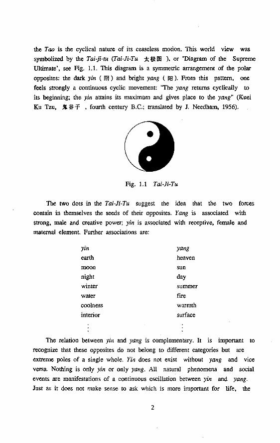
the Tao is the cyclical nature of its ceaseless motion. This world view was

symbolized by the Tai-ji-tu (Tai-Ji-Tu Ä &t lm ), or 'Diagram of the Supreme

Ultimate', see Fig. 1.1. This diagram is a symmetrie arrangement of the polar

opposites: the dark yin ( WJ ) and bright yang ( ~B ). From this pattern, one

feels strongly a continuous cyclic movement "The yang returns cyclically to

its beginning; the yin attains its maximum and gives place to the yang" (Kuei

Ku Tzu, _.tt--=f , fourth century B.C.; translated by J. Needham, 1956).

Fig. 1.1 Tai-Ji-Tu

The two dots in the Tai-Ji-Tu suggest the idea that the two forces

contain in themselves the seeds of their opposites. Yang is associated with

strong, male and creative power; yin is associated with receptive, female and

matemal element. Further associations are:

yin

earth moon

night

winter

water

coolness

interlor

yang

heaven

sun

day

summer

ftre

warmth

surface

The relation between yin and yang is complementary. It is important to

recognize that these opposites do not belong to different categones but are

extreme poles of a single whole. Yin does not exist without yang and vice

versa. Nothing is only yin or only yang. All natural phenomena and social

events are manifcstations of a continuous oscillation between yin and yang.

Just as it does not make sense to ask which is more important for life, the

2

is good is not yin or yang but the dynamic balance or harmony between the

two; what is bad or harmful is imbalance.

There were two most influential schools in old China: Confucianism,

founded by Kong Fu-Zi (Confucius, fL ~ -T , 551 - 479 B.C.), and Taoism,

founded by Lao Zi (Lao Tzu, :t -T , who was said to be 20 years older than

Confucius). Confucius studied social system; and he believed that in order to

keep the balance of the society there must be a strict convention of social

etiquette. One of the rules Confucius made for the people was that every one

in society should behave according his social position - an emperor should

act as an emperor, minister as minister, father as father and son as son

ti ti lif lif ~~-T-T ). He also advised people not to be extreme and

radical ( J:j:l ldf .:<::. J!t , moderation). Taoists studied more on the relation

between the human being and nature. The harmony of this system is achieved if

people can discover the tao, or the law of nature, acting spontaneously. Wu

wei ( x 1; ) is the action Taoists took; it means follow the nature and do not

act against nature.

In our time, when talking about social life and scientific research, the

following associations of yin and yang might be acceptable:

yin yang

feminine masculine

contractive expansive

conservative demanding

responsive aggressive

cooperative competitive

intuitive rational

synthesizing analytic

integral reductional

Examining this list of opposites, we see that at least since 300 years

ago, Western society and science have consistently favored yang over yin

(when compared with Eastern culture): compeuuon over cooperation,

exploitation of nature over conservation, rational knowledge over intuitive

wisdom, reduction over integration, analysis over synthesis, and so on.

After having recognized this imbalance, it is not difficult to understand

why Western scientists are so fond of forma! mathematics; why they are so

good in differentiating problems into their smallest possible components; and

why they often forget to put the pieces back together again. This imbalance

3

also shows that there is a need to emphasize more strongly yin in Western

research, i.e., to emphasize intuition, synthesis and integration.

Under such a guideline, in this work, we will try to integrate

identification and control for industrial manufacturing systems; we will show

how this philosophy can be useful for choosing a research topic and even for

generating new ideas.

In the last few centuries in the history, however, Chinese preferred yin

to yang (when compared with Western culture) - they would give response to

the nature rather than exploit it, they tried to follow the rules in order to

avoid conflicts, they preferred talking about general philosophy to the

completion of a concrete project, they preferred intuitive wisdom and common

sense to analytica! reasoning. This is perhaps one of the reasoos why modern

science has not been bom in China.

One might ask what modern China cao learn from Western culture. The

author believes that there is a need to emphasize yang. Por example, make

competition fair play and bring it into the public eye from underground; give

individuals more freedom and opportunities for self-fulfilment; use more

scientific reasoning and analytica! approach to study social, politica! and

economical problems; test theories by facts instead of by doctrines; and so

on. The science and technology in modern China, however, suffer the same

illness as in the West, that is, there is in general a lack of intuition and

integration approach. One of the reasoos is that most researchers in China

are in the learning period, we do not have enough experience and confidence

yet to go further to combine the Western and the Chinese approaches. Time and

an open policy are needed to achieve a good combination of the W es tem and

the Eastern approaches and, more broadly, their cultures. But if this

happens, there will be a renaissance of Eastern culture, which will be

enjoyed , this time, by both Eastern and Western people due to modern

communications. More discussions on this topic is beyond the scope of the

thesis.

1.2 The Philosophy of ldentification

There are basically two ways of building models of systems the

mathematica! modelling approach and the identification approach.

Mathematica! modelling is the most common and conventional method in

Western science and technology. By this approach one starts with decomposing

the system into its subsystems, and subsystems into their elements; then one

4

writes down the equations for each element based on first principles, e.g.,

physical laws; and finally one forms the system model by putting the

equations together according to the interrelations between the elements and

the subsystems. Some people also call this approach physical modelling. From

the methodological point of view, this is typically a reductional, rational

and analytica! approach; a yang approach.

System identification can be defined as deriving system models from

observations and measurements. In this approach, the system is viewed as a

whole; there is perhaps no need or intention to analyze each element of the

system; the systems behavior is observed by measuring some relevant

variables; and such a model is chosen of which the behavior fits best the

measurements. By this approach one does not attempt to go deep into the

system, the precise physical knowledge of the system elements and their

interrelations is not necessary; therefore identification is also called

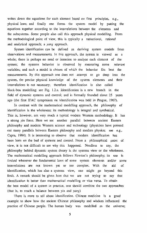
black-box modelling; see Fig. 1.2.a. Identification is a new branch in the

field of dynarnic systems and control; and is formally founded about 25 years

ago (the first IFAC symposium on identification was held in Prague, 1967).

In contrast with the mathematica! modelling approach, the philosophy of

identification is the wholeness; its methodology is integral and synthetical.

This is, however, not very much a typical modern Western methodology. It has

a strong yin force. Here we see another parallel between ancient Eastern

philosophy and modern Western science and technology (physicists have pointed

out many parallels between Eastern philosophy and modern physics; see e.g.,

Capra, 1984). It is interesting to observe that modern identification has

been bom on the bed of systems and controL From a philosophical point of

view, it is not difficult to see why this happened. Needless to say, the

philosophy behind dynamic system theory is the systems view or the wholeness.

The mathematica! modeHing approach follows Newton's philosophy; its use is

lirnited whenever the fundamental laws of some system elements and/or some

interrelations are not known yet or too complex. With the aid of

identification, which has also a systems view, one might go beyond this

limit. A remark should be given here that we are not trying to say that

identification is better than mathematica! modeHing or vice versa. To obtain

the best model of a system in practice, one should combine the two approaches

(that is, to reach a balance between yin and yang)

There is more to tell about identification. Chinese medicine is a good

example to show how the ancient Chinese philosophy and wisdom influenced the

practice of Chinese people. The human body was modelled .as the universe;

5

viewed as an organic whole and there are yin and yang parts. For example, the

back is yang, the front is yin; the skin or surface is yang, the interlor is

yin. lnside the body, there are yin and yang organs. Of the five viscera the

heart and liver are yang organs and the spleen, lungs and kidneys are yin

organs. The balance between yin and yang is maintained by a continuous flow

of qi (chi"' ), or vital energy, cyclically between yin and yang organs.

Whenever the flow between yin and yang is obstructed (hindered), an imbalance

will occur and the body falls ill. To detect the illness, pulse feeling was

the most important methad of diagnosis of Chinese medicine. The examinatien

is made upon both the right and left wrists, the physician using three

fingers (index, rniddle and ring fingers) to fee! the pulse of his patient. It

is recorded that Bian Qiao (Pien Chiao, Ai} ft!6 ) who lived about 255 B.C. was

a. Identification is black-box

modelling

1 oî 1s-B* 1 G-±. ,Q±

2. O·K

b. Performing a diagnosis

for his female parient

Fig. 1.2 The philosophy of identification

6

the inventor of this idea; cf. Wong and Wu, (1936). Before him the pulses

from many places of the body should be measured. But Bian Qiao realized that

one could gather enough înformation only from the two wrîsts of the patient,

which was much more convenient

One of the rules made by Confucianism was that men and women should not

be close with each other ( !f} :9: tJl ~ ;r- ffi: ), except within the family; and

an unmarried girl should not be seen by male outsiders. But this rule was not

really a restrietion for a Chinese doctor to perfarm diagnosis for his female

patient. In such a case, he could simply feels the pulses of the lady behind

the curtain; see Fig. 1.2.b. This procedure, however, fits very well to the

definition of îdentification; and we note that the doctor was identifying a

three output system! This story of pulse feeling suggests that the history of

system identification is at least 2000 years longer than we usually think.

So much about philosophy. Let us now turn to more practical and technica!

issues.

1.3 Defining and Analyzing the Probierus

In the 1980's, due to the world-wide competition, shortage of natural

resources and pollution of the environment, an industrial manufacturer has to

face following challenges:

decreasing delivery times;

increasing demand on product quality;

large variety but smaller series of products;

more constraints on material consumption, energy consumption, and

pollution;

Research on and development of advanced process control systems is one

way to meet such challenges. To this end, many disciplines, such as

modelling, identification, systems and control, microelectronics,

informaties, measurement and sensors, physics and chemistry, need to be used

jointly. It is obvious that we are forced to combine things when solving

practical problems. This is also feasible because most of the fields

mentioned above have experienced a fast development in recent years and much

work has been done on the fundamentals. The main problem is how to put these

pieces together. Due to my academie background and personal interests, the

interalation of two pieces - identification and control - will be studied

m this work.

A wide class of industrial manufacturing plants can be characterized as

7

follows: They are multi-input, multi-output (MIMO) processes.

Modelling by physical laws is only partly feasible or, in other

words, physical modelling alone can not supply a model that is

suitable for control; so identification, that is, denving a process

model from experimental data, is necessary for obtaining a model to

be used in the controller design.

The process dynamics is highly complex, e.g., nonlineacity and time

varlation might occur, and there are process disturbances. These

cause model uncertainties (modelling errors). But still linear and

time invariant models will give good approximations of the process

dynamics at each woricing point

Time delay(s) exist(s) in the process under study; the plant is often

a nonminimum-phase process.

Disturbance attenuation and stability robustness are the main desired

features of the controlled system.

Example 1.1 A glass tube production process (Back:x, 1987).

The process oudine is shown in Fig.1.3. By indirect electric heating the

glass is melted and flows down through a ringshaped hole along the accurately

positioned mandril. The glass tube is pulled down due to gravity and

supported by a drawing machine.

Shaping of the tube takes place at, and just below the end of the

mandril. The longitudinal shape of the tube is characterized by two important

parameters, the averaged wall thickness and averaged diameter, which will be

taken as the process outputs to be controlled. Both of these dimensional

variables are influenced by many process variables:

- the mandril gas pressure,

- the drawing speed,

- the power applied to melt the glass,

- the pressure in the melting vessel,

the composition of raw materials,

- the room temperature,

- and others.

Among these variables, the mandril pressure and the drawing speed can

affect the wall-thickness and the diameter most direcdy and easily, with the

shortest delay times and over the widest frequency range. Hence the process

is modelled as a two input (mandril pressure and drawing speed) and two

8

output (wall-thickness and diameter) process with the other variables being

treated as disturbances. Large time delays exist because the measurement of

the tube dimensions (process outputs) is only possible after the tube has

caoled down to sufficiently low temperatures.

NEEDLE POSITlON IX,Yl

PRESSUftE MEL TI NG VE55EL

POWER SUPPL Y

Fig.1.3 Outline of the glass tube production process

The purpose of the study was to develop a computer controVsupervision

system in order

(1) to reduce the variations of the dimensions at a working point (increase

product quality), and

(2) to automate the change-over between different wor.ldng points and

decrease the change-over time (make production more flexible).

The mathematica! modeHing of the process would result in two partial

differential equations with some important parameters being unknown.

Experience has shown that it is more appropriate to use identification

techniques to derive approximate linear, lumped parameter models of the

process at various werking points from the experimental data, and to design

or adjust the control system based on estimated models. In this approach

mathematica! modeHing can supply a priori knowledge about the process for

the identification and parameter estimation. •

More details about the glass tube production process and discussions on

the characteristics of industrial processes can be found in Backx (1987); abd

we will come back to this process in Chapter 6.

9

1.4 Scope of This Thesis

For such class of industrial processes, control theory and design

techniques that can cope with model uncertainties will be more suitable than

the conventional approach. This topic, usually · called robust control, bas

been studied extensively since 1980. For the analysis and ·design of a . robust

control system, one needs not only a nominal model of . the process but also a

suitable description of the model uncertainty, typically, an upper bound of

the modelling errors in thè frequency domain.

Thus, it is clear that an estimation of the uncertainty of identified

roodels in the frequency domaio will be the key to linking identificati_on and

robust controL This topic, however, bas not received enough attention; most

of recent research on identification bas been focused on time domain

parametrical estimation methods and convergence analysis. Based on these

observations, we decide to deve/op an identification method which de/ivers a

nomina/ model tagether with an upper bound of its errors in the frequency

domain; this should be applicable for industrial processes. This forms the

first part of the work (Chapter 2, 3, and 4).

Here, the idea of integration has motivated naturally such a research

topic. Choosing a research topic might be one of the most difficult parts of

research. Many researchers chose topics based on reductionism: split a

problem into its smaller pieces and analyze deeply one such piece. Here we

can say that the opposite is also possible (even commendable), that is, to

put pieces back together again.

Often identification experiments have to be performed in closed loop,

that is, under feedback control, due to safety and/or economical reasons. It

is well k:nown that, compared to an open loop experiment, there is a

degradation of process model quality when using closed loop data. In this

structure, there is a conflict between identification and control; and the

estimation algorithm may even be unsuccessful (not converge) when the open

loop process is unstable or nearly unstable, which is often the reason for a

closed loop experiment. But,

when viewing identification and control as two aspects of the same

problem rather than two separate problems,

when viewing the closed loop system as a whole,

a question arises: for control system design or adjustment, is it rea//y

necessary to identify the origina/ process dynamics when it a/ready be/ongs

to a c/osed loop system? By answering this somewhat philosophical question,

10

we arrive at a new and natura! solution to the problem: first identify the

closed loop system dynamics, then design a secend loop controller based on

this system model. The model of the original process is not needed for the

design of the second loop controller. This approach is studied in Chapter 5,

which ·is the second part of the work. ~n the new scheme, identification and

control are mutually supporting; there is no need to develop new

identification and control techniques for the scheme.

There is another question to be asked: why such a simple solution for

combining identification and control has not been proposed for so many years?

Perhaps it is not because that it is too simple to mention. The reasen might

be that most researchers fellow Newton' s reductionism: they tend to start

with studying the smaller pieces of the original problem, even when it is not

necessary. Taoists said, the more you know about tao, the more you can

achieve with less effon.

If one wants to know how the ideas work, please read the following

chapters.

11

Chapter Two

ASYMPTOTIC PROPERTIES

OF BLACK-BOX MIMO TRANSFER FUNCTION ESTIMATES

2.1 Introduetion

This chapter presents a study of some properties of identification in the

frequency domain. The asymptotic theory of MlMO transfer function estimation

will be developed. First the metbod of speetral analysis for transfer

function estimation will be studied. The result is asymptotic both in the

number of data and the model order. Then a similar result is derived for thé

MlMO transfer function estimates obtained by preelietion error methods, where

no structure or order is chosen a priori and we allow the model order to

increase when the number of data increases.

This work extends the recent aymptotic theory of Ljung and Yuan; cf Ljung

(1985), Ljung and Yuan (1985) and Yuan and Ljung (1984); and paves the way

towards the estimation of a nominal model as well as a upper bound of

transfer function errors of MlMO models, which will be the contents of the

next chapter. Secdon 2.2 treats the speetral analysis. Section 2.3 derives

the covariance expression of predierion error models in the frequency domain.

Before finishing the introduction, some preliminaries will be given.

Consider a discrete-time process with m inputs and p outputs. A set of

general linear time-invariant models for the relationship between inputs and

outputs can be written as:

y(t) = L g(k)u(t-k) + v(t) (2.1.1) k=1

where: y(t) is a p-dimensional column output vector at time t; u(t) is an

m-dimensional column input vector at time t, and its properties will be

described later; g(k) is a sequence of pxm matrices (Markov parameters); and

{ v(t)} is a p-dimensional stochastic stationary process with zero mean

val u es.

When the unit time delay operator q-1 is introduced:

q'1u(t) = u(t-1)

the model (2.1.1) can be written as

12

y(t) = G(q)u(t) + v(t) (2.1.2)

where 00 k

G(z) = L g(k)z- (2.1.3) k=l

is called transfer operator of the model.

The transfer function matrix of the model is:

G(eiro) = Ï g(k)e-irok -1t ::> ro s 1t (2.1.4) k=l

For the model output disturbances, a common approach is to assume that

they are filtered white noises:

where

v(t) = H(q)e(t)

H(z) = Ï h(k)z-k k=o

h(k) is a sequence of pxp matrices with

h(O) = lp (pxp idenrity matrix)

(2.1.5)

(2.1.Sb)

and { e(r)} is a p-dimensional white noise vector with covariance matrix R.

Both H(q) and H 1(q) are stable. Then {v(t)) will be a stationary process

with speetral density

00 • • •

<l\(ro) = L [ E{v(t)vr(t-t)}le-1rot = H(elfJ))RHT(e·1ro) (2.1.6) t=-oo .

where E means expectation, r means transpose, H(e1~ is the transfer function

matrix of H(q):

H(ei~ = Ï h(k)e-irok -1t s ro s 1t (2.1.7) k=o

The problem of identification is to estimate an approximate model from

observed input-output data. Denote the data sequence by z!':

z!' = y(l ),u( 1 ), ... . .. , y(N),u(N) (2.1.8)

Assume that the true process can be described by

y(t) = G (q)u(t) + H (q)Ç(t) (2.1.9) () ()

0 where ( Ç(t)} is a white noise vector with covariance matrix R. Moreover,

G (q) and H (q) are stabie filters. The output noise spectrum is then 0 ()

(2.1.10)

13

In (2.1.9) the inputs are noise free. This is a realistic assumption because

in practice, in a open loop case, the inputs are often generated by the

computer and applied to the actuator, which is modelled as part of the

process; these signals neither have computer round-off errors nor and nor do

they suffer from disturbances. Process · disturbances as well as measurement

noises are accounted for in v(t).

Denote G(i~ as the model transfer function matrix, then G (i~ can be . 0

represented as .

where L\(ei~ is called additive modeHing errors (pertutbation). Similarly,

for the entries of G (i~, we have 0

im... A iro iro Goi/-e J = Gi}e ) + L\i}e )

where A .. (i~ is called the element additive modelling error; note that it IJ •

is preeisely the (iJ) element of A(i~.

(2.1.11)

(2.1.12)

In practice the true transfer function matrix G (iro) can not be 0

identified exactly beeause of the disturbances, and the limititions on the

experiment and model complexity . Recent theoretica! results have shown that

the nominal process (plant) model and upper bounds of the modelling errors in

the frequency domain are needed for studying the robustness of a feedback

controlled system; cf. Doyle and Stein (1981), Owens and Chotai (1984),

Vidyasagar (1985) and Kouvaritakis and Latchman (1985a, b). So the problem of

identification for robust control consists of: (1) the estimation of the

nomina! model and (2) the estimation of an upper bound of the modeling error.

2.2 Speetral Analysis Method

For industrial process identification, we can often enjoy the luxury of

designing the input signals for the experiment, and having a large number of

data; the disturbances, on the other hand, will often be a main cause of the

model uncertainty. In such a situation, the speetral analysis can be a

natura! nonparametrical method for the estimation of transfer functions.

Speetral analysis has been studied extensively in the field of time

series, cf. Jenkins and Watts (1968) and Brillinger (1975). The transfer

function matrix of a MIMO process can be estimated row by row. The i-th row

of the transfer matrix can be estimated by the following steps:

Calculate the auto- and cross-correlation function estimates:

14

(mxm matrix) }

't = -n,-·,0,-·,n

(mxl vector)

(2.2.1) _N 1 N K~y. ('t) = N I Yj(t)U(t-'t)

l t I

Take the Fourier transform:

ct>~(ro,n) r R~(t)e·i'tro 't = -n } -1t ::;; 0) ::;; 7t

~ y . (ro,n) == r R~y. (t)e- i 'tro 1 't = -n 1

(2.2.2)

Calculate the transfer function estimates:

(2.2.3)

In order to make a comparison with the parametrical method, which will be

stuclied later, we will cal! 2n+ 1 the "order" of this model because it will

show up in the expression of the covariance matrix of the transfer function

estimates. The computations of R~(t), and R~Y/'t) may involve inputs and

outputs prior to the first, and after the N-th sample moment. For the

analysis, these values can be replaced by zeros or by other bounded numbers.

They will not influence the asymptotic result. A better alternative is

offered, however, by taking these values to be the real measurements. This

can be realized by collecting the data sequence z!l+2n instead of zN:

zN+2n :== y(-n+l), u(-n+I), ... , y(N+n), u(N+n)

and computing R~('t) and RN (t) according to (2.2.1). uyi

Denote y0(!) as the noise free outputs, then from (2.2.1) we have

~/'t) == R~y~('t) + ~v.('t) I I I

We can see that for an open loop experiment,

~v.('t) ~ 0 as N ~ "" I

This implies that the influence of { v(t)} on the estimated cross- correlation

functions will be averagecl-out when the number of data N is large.

IS

In order to give a quantitative description of the estimates (2.2.3) we

need the following

Formal Assumptions: Cl: The real process is bounded-inputlbounded-outpUt stable, that is

00

L lg~.(k) I < 00 'ViJ k=1 IJ

C2: The disturbances are filtered white noises as in (2.1.9), where {l;(t)}

is white noise with covariance matrix R , and unifonnly bounded 0

fourth moment, and both H (q) and H- 1(q) are stable. 0 0

From C2, one can show 00

E[v(t)vr(t-t)] =: Rv(t), I: I t luRv(t)ll < oo

t =-"'>

where E denotes the mean value expectation, and 11·11 denotes any matrix

norm, and 00 •

<l>v(ro) := I: Rv(t)e·ttro. u v(ro)u < C (a constant) 'Vro 't=-00

C3: {u(t)} is independent of {v(t)} and llu(t)ll ~ C1

(a constant) 'Vt

C4: u(ro) := I im <l>~(ro,n) exists N~.n~

CS: amax«<>iro)) ~ C2

(a constant), amin(<l>u(ro)) ~ 8 > 0 'Vro

2n C6: ~ I: h lu~(t)ll ~ 0 as N ~ oo, n ~ oo

t=-n C7: n ~ oo as N ~ oo

Remarks: -Cl and C2 are common assumptions in the field of identification. We

wil! show in Chapter 5 how to solve the difficult problem of identification

of even an unstable process , i.e., when Cl does not hold for the original

process.

C3 implies that the identification experiment is performed in open loop.

For closed loop experiment, the speetral analysis will not give consistent

estimates, due to the correlation between the disturbances and the process

inputs; in this case the prediction error method can be used.

C4 and CS wil! hold when input signals are generated by stationary

stochastical processes, which are ergodic; and which are persistently

exciting with order infinity. This signa! is deterministic and is called

16

quasi-ationary signal (Liung, 1987).

C6 means that the auto-correlation functions of the inputs decay

sufficiently fast.

C7 means that we allow the "order" (2n+l) to go to infinity when the

number of data tencts to infinity, but N goes to infinity much faster than

(2n+ 1) does; this is the meaning of C8. •

Theorem 2.2.1: Consicter the estimate G7(eiro) = [G71(eiro) ... G7m(eiro)]

obtained from (2.2.1) - (2.2.3). Assume that Cl - C8 hold. Then

as N ~ oo Vro (2.2.4)

(asymptotic unbiasedness)

where G .(eiro) is the i-th row of G ei~. ~ 0

/ N A n iro 2n + I [G i(e ) (2.2.5)

(asymptotically normal distribution)

where AsN denotes asymptotically normal distribution.

The proof is given in Appendix 2.A.

Due to the nice structure of this result, we know immediately the

properties of each transfer function estimate:

Corollary 2.2.1: Consicter the estimate G7/eiro) obtained from (2.2.1) -

(2.2.3). Assume that Cl - C8 hold. Then

•

IE{ G~ .(eiro)} - G .. (eiro) I ~ 0 IJ olj

as N ~ oo (2.2.6)

Some Comments on the Results

The first part of Theorem 2.2.1 says that the transfer function estimates are

asymptotically unbiased; from (2.2.7) the varianee of each transfer function

estimate is

(2.2.7)

•

A n iro 2n + 1 · · 1 var[G i/e )] = N I cl> u (ro)]i/cl> v/ro)) (2.2.8)

which will decrease when the number of data N increases. This remarkably

17

simple expression has a clear physical meaning: it says that the varianee of

each transfer function estimate at a particular frequency is asymptotically

given by the (generalized) noise-to-signal ratio at that frequency multiplied

by the ratio of model-order-to-number-of-data. Combining (2.2.6) and (2.2.7)

gives the consistency of the estimates. This theory not only brings us

theoretica! insight into identification, but also supplies the applicable

formula for the calculations. The result can be used for optimal input signal

design (see Yuan and Ljung, 1984); and it can also be applied to obtain an

upper bound of the modeHing errors, which is explained in the next chapter.

2.3 Prediction Error Method

During the previous two decades, the theory and techniques of system

identification have developed rapidly and many sophisticated time domain

parametrical methods have been proposed and studied. Many of these methods

can be classified as belonging to the family of predierion error methods,

which will be introduced in the following.

Let model (2.1.1) be parametrized in some way:

y(t) = G(q,8)u(t) + H(q,8)e(t) (2.3.1)

where 8 is a d-dimensional parameter vector. Asuuming {e(t)} is white noise,

we can determine the one step ahead prediction from (2.3.1):

;u I 8) = [IP - 111(q,8)]y(t) + H 1(q,8)G(q,8)u(t) (2.3.2)

by defining the predierion error

;(t) = y(t) - ;(tI 8) = H'1(q,8)[y(t) - G(q,8)u(t)] (2.3.3)

Then a common way to determine the parameters is to minimize the squared sum

of the predierion errors (an maximum likelyhood estimation if { e(t)} has

Gausian distribution):

(2.3.4)

where

1 N ~ ~ YJI.-8) = N 2. eT(t,8)e(t,8)

t =I

and D n c Rd is the parameter space. Here the subscript N is to emphasize that

N samples of data are used for the estimation; n is the model order which

will be defined later; the dimension of the parameter space d depends on the

numbers of process inputs and outputs, the model order and the model

18

structure.

The general description (2.3.1) - (2.3.4) can cover most of the time

domain identification techniques in practice. Specific methods can be

obtained by taking a specific model structure; see, e.g., lanssen (1988).

After the parameter estimation, the transfer function estimates are

~J;;(e~~ = G(~}/n), i 00) }

H;:;<i~ = H(8}/n), e1~ (2.3.5)

Recently, Ljung and Yuan developed a theory on the properties of the transfer

function estimates. In Ljung and Yuan (1985), it was shown that in SISO

cases, for the Markov parameter model (impulse response model), the varianee

of the transfer function estimate is proponional to the noise to input

signal ratio, multiplied by the ratio of model order and number of samples.

The extension of this result to MIMO Markov parameter models can be found in

Yuan and Ljung (1984). In Ljung (1985), it has been shown that the same

result holds for the polynomial-type of SISO models, e.g. ARMA model or ARMAX

model. This section extends the result of Ljung (1985) to MIMO

polynomial-type models, estimated by the prediction error method.

In Section 2.3.1 the Box-Jenkins model wil! be introduced and the shift

property of the polynomial-type models wiJl be emphasized. The main result is

developed in Section 2.3.2.

2.3.1 Black-Box Models and Shift Property

In order to show the idea in a concrete way, we present a special model

structure here. This model is given as

G(q,8) = A -I (q,8)B (q,8) }

H(q,8) = C 1(q,8)D(q,8) (2.3.6)

where A(q,8), B(q,8), C(q,8) and D(q,8) are polynomial matrices with

dimension pxp, pxm, pxp and pxp respectively:

A(q,8) : lp + A1q

-l + ... +A q-n n

) B(q,8) Blq

-1 + ... + B q -n

: n (2.3.7)

C(q,8) = lp + C1q'1 + + C qn

n

D(q,8) = lp + D1q-1 + ... + D q-n

n

(2.3.7) is a special form of the Box-Jenkins model with

19

A = I B = 0 C = I and D = I 0 p' 0 ' 0 p 0 p

(2.3.8)

Por this choice A0

= I, [A(q,9), B(q,9)] is called a monic ARMA model of

G(q,9). It can easily be shown that any ARMA model can be transformed into

the monic ARMA model provided A0

is invertible. B0

= 0 means that G(q,9) is

strictly proper; and th~s assumption is justified by the fact that most

input-output processes are strictly proper indeed. C0

= D 0

= I means that

H(O) = I as in (2.1.5b).

The order of the model (2.3.7) is n, which is the degree of the

polynomials in A, B, C and D matrices. Notice that here the order n is in

general not equal to the McMillan degree of the model; the McMillan degree of

model is defined as the dimension of the minimal state space realization of

the model .

Now we define the parameter vector as

9 = col [A 1 B1 C1 D1 A

2 B

2 C2 D

2 ••• An Bn Cn Dn]

e, 92

(dxl) ( d = np(m + 3p )

where col[·] denotes the column operator, see Appendix 2.B, and

(sxl) for k == 1, ···, n

(2.3.9)

(2.3.10)

Here d is the number of parameters, d = ns, and s = p(3p + m) for the Box

Jenkins model.

Let

T(q,9) := col[G(q,9) H(q,9)]

=

a,, (q,e)

?pm(q,9)

/{I I (q,fJ)

/{pp(q,9)

((p(m+p))xl)

where Gij(q,9) and Hf/q,9) are the {iJ) entries of rational matrices G(q,9)

and H(q,9) respectively. It is easy to verify that

20

(2.3.11)

where

aTT (q,8) = q·kzc 8) ae q, k

Z(q 8) ._ (}TT (q,8) . q · ·- ae

I

(2.3.12)

(sxp(p+m)) (2.3.13)

This holcts because G .. (q,8) and H .. (q,8) are ration al functions of q'1 and 8 l] l.J

is decomposed as in (2.3.9). The reader can verify (2.3.12) by taking a SISO

ARMA model as an example. Equation (2.3.12) is the so called "shift property"

of model set (2.3.6) and (2.3.7), which is one of the keys for deriving our

result.

At the end of this section, a gradient of the prediction is introduced

which will be important for deriving the asymptotic distribution. We will

give an expression which is convenient for our purpose. Let

(dxp)

From (2.3.2) it follows that

H(q,8)y(t I 8) = H(q,8)y(t) - y(t) + G(q,8)u(t)

According to relation (2.B.6) in Appendix 2.B, we have

and in a tranposed version:

T (col[G(q,e)]) [u(t)®l P 1

- y~'(t) + (coliH(q,e)])'~'[y(t)®l P]

(2.3.14)

(2.3.15)

(2.3.67)

(2.3.17)

where ® denotes the Kronecker product; see Appendix 2B. Using (2.B.8) we

obtain the relation for the gradient with respect to 8:

d T · d T = (ffi(col[G(q,8)]) [u(t)®lp] + (ffi(col[H(q,8)) [y(t)®lp] (2.3.18)

Using the properties of the Kronecker product, it can be shown that

21

[/ ®jT(tiB)] dHT(q,9):: d(co/[H(q,9)])T rJ(t!B)®/] p ae aa P

Substituting (2.3.19) into (2.3.18) leads to

where -T means inverse and transpose, and

Ç(t,9) = [ ~(t) ] • ~(t,O) = y(t) - y(t I 0) e(t,9)

It is also easy to show that

[Ç(t,9)®Jp)lfT (q,9) = [/ m+p ®lfT (q ,9)) [ Ç(t,9)®/ p)

Then (2.3.20) becomes

2.3.2 Asymptotic Properties of Prediction Error Models

(2.3.19)

(2.3.20)

(2.3.21)

(2.3.22)

In this section the main result will be developed. First some forma!

assumptions will be given. Then several lemmas will be proved. Finally, we

will end up with Theorem 2.3.1 which gives the expression of the covariance

matrix of the transfer function estimates. Readers who do not like the

tedious technica! details can skip Section 2.3.2.(1) and Section 2.3.2.(2),

and start reading from Theorem 2.3.1.

(1) Some Assumptions

Estimating a transfer function matrix is basically a non-parametrie problem.

Since the process is viewed as a black box, the intemal parametrization via

9 is merely a vehicle to arrive at this estimate. Then, we let the model

order n depend on the number of observed data

n = n(N) (2.3.23)

in order to get the best transfer function estimates. Typically, we allow

n(N) to tend to infinity when N tends to infinity:

22

n(N) -7 oo as N -7 oo (2.3.24)

When the model order n increases, the model may lose "parameter

identifiability", but it wil! retain "system identifiability" under weak

conditions on the experiment design; see Gustavsson et al. (1977) for a

discussion of this point. To deal with this problem, we introduce a

regularization procedure in the following way. Let

(2.3.25)

where

• A 1 N • A

Ef?(t,8)e(t,8) 1 im N :2: Eer(t,8)e(t,8) N-700 t = 1

(2.3.26)

Assume this is a convex function. Here n emphasises that. the minimum is

carried out over n-th order models. Now define the estimate 8N(n,a) by

(2.3.27)

where

1 1 NAT A v ~e(n),a) := 2 [N :2: e u.e)e(t,S) + ace - eYce - e·)]

t 1

(2.3.28)

If the function in (2.3.26) is convex, then V N(S(n),a) is strictly convex

which leads to the uniqueness of the minimization in (2.3.27). Here a is a

regularization parameter, helping us to select a unique minimizing element in

(2.3.27) in those cases where a = 0 leads to non-unique minima. The procedure

here is a technica! way of dealing with the unique estimate

A iro iro A ico A

GN(e ) = G(e ,eN) l im G(e ,8(n,o)) 0-?0

(2.3.29)

by a sequence of unique parameter estimates { eN(n,o)), rather than by the

possibly non-unique (but realizable) estimate SN

Further assumptions

Assume that the true system can be described by

y(t) = G (q)u(t) + H (q)Ç(t) 0 0

(2.3.30)

where { Ç(t)) is a white noise vector with co varianee matrix R and bounded 0

fourth moments. Moreover, G (q), H (q) and H'1(q) are stable. The output 0 0 0

23

noise spectrum is then

~ (ro) = H (i~R HT(e-i00) (2.3.31) V o o o

Assume the predietor filters f{1(q,e) and f{1(q,e)G(q,e) in (2.3.2), along.

with their frrst-, second-, and third-order derivatives with respect to e, are unüormly stabie filters in e e D n for each given n. Let

T~(i~ = T(eiro, e·(n))

A iro i()) A

Tn<e ,n,o) = T(e , eN(n,o))

T (i~ = col [ G ( eiro) H (ei00)] 0 0 0

} Assume that

n~

which implies that T~(ei~ tends to T0 (ei00

) as n tends to infinity.

In the same way as Z(q,e) defined in (2.3.13), we denote Z (q) as 0

êJTT(q) I Z (q) := - 0

- ·q (e is the true .parameter vector) o ëJe e=e 0

I o

and in frequency domain:

. ëJTT ( eiro) . Z (ez~ = o .iro

o ëJe 1

Assume that

z~ci00.e) Z0(ei00,e)

Further, assume that

is invertible

N Ru('C) := Eu(t)uT(t-'C) := I im k L Eu(t)uT(Fc)

N~ t=t

exist and that

for 'C < 0

Define the spectrum ( ro) and <l> ( ro) as u ue 00 •

 u(ro) := L Ru('t)e·lWt 'C = .oo

24

(2.3.32)

(2.3.33)

(2.3.34)

(2.3.35)

(2.3.36)

(2.3.37)

(2.3.38)

(2.3.39)

Finally, assume that

1 N d A A

I i m :E E [OEf eT(t,8)e(t,8) / • ] = 0 (n fixed) N--700 VN t = 1 8=8 (n)

(2.3.40)

Comments on the assumptions

Most of these assumptions are similar to, or the same as, the assumptions Cl

CS given in the previous section; hence the remarks given there can be used

to understand the physical meaning of the assumptions here. Note, however,

there are two important differences: (1) no Jonger do we assume an open loop

experiment, this implies that the results derived later wil! hold for closed

loop experiment as wel!; (2) in the last section, the consistency of the

transfer function estimates is a result that is given by Theorem 2.2.1, but

in this secdon it is taken as an assumption in (2.3.33) (in another form);

the proof of the consistency of prediction error models can be found in Ljung

(1987) and Söderström and Stoica (1989).

(2) Teehoical Lemmas

Now let us start the denvation of the expression for the covariance matrix

of the transfer function estimates. Denote X(t-1 ,8) as the sxp dimensional

process

Z(q,8)(/ ® H·T(q,8))(Ç(t-l ,8)®/p) ln+P

(2.3.41)

where

(2.3.42)

Then from (2.3.22) we have

[

X(t-1,8) l xCt-2,8) 'lf{t,8) = :

xu-n,8)

(2.3.43)

Denote the dxd matrix

25

.ê'lv(t,I:J)'IfT(t,I:J) =: M n(I:J)

It consists of nxn blocks each of dimension sxs, and the (k-J)th block is

Ex(r-k,e)-l(t-j,I:J) =: r X(j-k,6)

M (6) is called the block Toeplitz covariance matrix of the process X(t,I:J). n Introduce the sxn matrix

W (ro) = [i00I ii00I ... enirol ] n s s s

Then the spectrum of X(t,I:J) is

(2.3.44)

(2.3.45)

(2.3.46)

<t>X(ro,e) = ~~ ~ Wn(ro)Mn(O)W~(-ro) (2.3.47)

and, from (2.3.41) and the properties of the Kronecker product, it follows

that

o ÎOO T Î(l) 0 0 tl:ft 1 Î(l) 0 T -iOO o <l>X(ro,v) = Z(e ,0)[/m+p®lf (e , )][<l>ç(ro, )®lp][lm+p'Cilf (e , )]Z (e ,v)

(2.3.48)

where <l>ç(ro,I:J) is the spectrum of Ç(t,I:J) which is defined in (2.3.20).

The idea of the denvation is to find the counter part of the known time

domain results (see, e.g., Ljung, 1987, Chpter 9) in the frequency domain.

The ftrSt lemma builds a relation between the time domain and the frequency

domain.

Lemma 2.3.1 Assume that (2.3.36)-(2.3.40) hold. Suppose also that

C ~ a (<l>u(ro)) , a . [<l>u(ro)l ~ ll > 0 max mm

(2.3.49)

where 0' , a . denote the maximum and the minimum singular values of the max mm

matrix respectively; and

l Ï_ l·d IIR (t)ll ~ 0 ..;;;. t ... n u

as N ~ ""• n(N) ~ oo (2.3.50)

Let Ad (n)={aij} be an arbitrary dxd matrix whose entties depend on n(N)

such that

and

1 im supnAdn ~ C n~

26

as n(N) ~ "" (2.3.51)

(2.3.52)

Then if n(N) -> oo as N -> oo

I im k Wn(w)[Mn(9) + 8Idr1AdW~(-w) [X(ro) + 8Isf1A(ro) (2.3.53)

n~

This result can be roughly understood as: the product of two Toeplitz

covariance matrices in the time domain corresponds to the product of their

spectrum matrices in the frequency domain. Condition (2.3.49) means that the

input spectra are bounded and persistently exciting with infinite order;

condition (2.3.50) means that the autocorrelations of the inputs decay to

zero sufficiently fast; and note the similarity between (2.3.50) and C6 in

the last section.

Proof: The matrix [M n(9) + 81 d] is the block Toeplîtz covariance matrix of

the sxp dimensional process

X(t,9) + va w(t)

where w(t) is an sxp dimensional white noise process with

r = Ew(t)wT(t) = I . w s

s '

•

The spectrum of this process is given by [X(ro) + 81 ]. The result follows

from the corollary to Yuan and Ljung (1984) Lemma 4.3. (Take WJW) = Wn(w),

~d = Mn(9) + 8Jd). o

Similarly we have

Corollary 2.3.1 Under the same conditions as in Lemma 2.3.1, then

I im ! W (w)Ad[M (9) + 8/dr1WT(-ro) = A(ro)[X(ro) + 81 f 1

n n n · n s n~

(2.3.54)

Let us now consicter the parameter estimate (2.3.27). First, from (2.3.25)

and (2.3.27) we have as in Ljung ( 1987)

êN(n,8) -> 9\n) w.p.l as N -> oo (2.3.55)

From the definition (2.3.27) and Taylor expansion, we have ' o = VN(9(n),o)

= V iv<e* (n),8) + VN(I;N(n),8)[êN(n,O) - e"(n)] (2.3.56)

where s~n) belongs to a neighborhood of e·(n) and from (2.3.55)

27

•

lim ~~~n)-e*(n)l =0 w.p.l N_",-

Hence

(2.3.57)

(2.3.58)

We shall consicter each of the factors of the right-hand side of (2.3.58)

in the following lernmas, where the results are expressed in the frequency

domain.

For the proof of the following lemma, we introduce A • •

e(t,a (n)) := ~(t) + r(r,e (n))

From (2.3.33) we have

E[rT(t,9*(n))r(t,9*(n))] ~ C! jn2 , lim C = 0

n_",- n

Lemma 2.3.2 Under previous assumptions and (2.3.60), then

The proof is given in Appendix 2.C.

Lemma 2.3.3 Under condition (2.3.60) and previous assumptions we have

where

v'N [V,N(9*(n),a] e AsN(O,Q(n)) as N ~ oo

=Z(i00,e*) ( (bç( ro,e*)®[/1 r <i00,e•)R 111 <i00,e·)] }Zr(e-iro,e·)

=:(/) xR<ro>

The proof is given in Appendix 2.D.

Combining these two lemmas we obtain the following result:

Lemma 2.3.4 Under all the previous conditions we have

. v'N [6~n,a) - e• (n)J E AsN(0,1<(n,Ö)) as N ~ oo

28

(2.3.59)

(2.3.60)

(2.3.61)

(2.3.62)

(2.3.63)

•

(2.3.64)

•

where

(2.3.65)

• Proof: (2.3.58) anct Lemma 2.3.3 imply that (2.3.64) holcts with

(2.3.66)

Applying Lemma 2.3.2, Lemma 2.3.1 and Corollary 2.3.1 successively, we obtain

then (3.2.65). a

Now we consicter

m rr ~et00,n,o) - r· cet00,n)J

By Taylor expansion

' iro s: • iro iro ' s: iro • T ~e ,n,o) - T (e ,n) = T(e ,9N(n,o)) - T(e ,e (n))

= -;r(ei00,e\n))lêN(n) e·(n)l + O(nêN(n) - e·(n)ll) de

(2.3.67)

(2.3.68)

Thus (2.3.64) implies that the variabie in (2.3.67) will have an asymptotic

normal ctistribution with covariance matrix

d iro • d T -iro • f>(ro,n,Ö) = -rT(e ,e (n))-R(n,Ö)·- T (e ,e (n)) de de

Now consicter the p(p+m)xd matrix

..!!....rci00 9) = [ ..!!...T(i00 e) ..!!...T(ei00,e) deT • de·;· • cte~

Using the shift property (2.3.12) it follows that

Anct using (2.3.46) we have

-4T(i00,e) = zT(ei00,9)Wn(-ro)

de Notice the minus sign in W n< -ro).

Combining (2.3.69) and (2.3.72) gives

29

(2.3.69)

(2.3.70)

(2.3.71)

(2.3.72)

P(ro,nl>) = zT(eiro,e•)w n(-ro):R(n,o)W~(ro)Z(e-iro,e•)

According to Lemma 2.3.4 and the fact that ~(t,e• (n)) -7 ~(t), we get

I im ! P(ro,n,o) = zT(i~[Z (é~s(-ro)ZT(i~ + of f 1•

n~n o o . o s

z (e·i~SR(-ro)ZT(i~-[Z (e·i~S(-ro)ZT(ei~ + OI r 1z (e·i~ 0 0 0 0 ~ 0

where, by suppressing arguments,

Consicter the limit of (2.3.74) as o -? 0. Apply the matrix inversion

lemma

to

and suppressing arguments and indices

[ZSZT + al]'1Z

= [~I - ~(as-t + zTz) -tzT]z

= ~ - Azra<zTz)· 1s 1 + n· 1 (zTzr 1<ZTZ)

se [small 0] !!! ~- lf[l - ocZTZ)" 1S- 1]

= Z ( Z T Z) - 1 S- 1

Hence the limit of (2.3.74) as o -? 0 is

s·1(-ro)SR(-ro)S'1(-ro) = <bj: 1(-ro)®[H <i~R HT(e"i~] " 0 0 0

= <t>((ro)®<bv(ro)

Now it is the time to state

(3) The Main Results

(2.3.73)

(2.3.74)

(2.3.75)

(2.3.76)

A iro Theorem 2.3.1 Consicter the estimate T N(e ,n,o) under the assumptions

(2.3.24)-(2.3.40), (2.3.49) and (2.3.50). Then

m [T ~i00,n,o) - T0

(eiro' n) 1 E AsN(O, P(ro,n,o))

as N -? oo for fixed n,o

30

(2.3.77)

where

I im I im ! P(ro,n,8) ~o n-Y><> n

u u.., ® <Il (ro) [

$ (ro) $ 1:(00) l-T <Ill' ( W) R V

(2.3.78)

..,u 0

This result is very genera!. It covers most of time domaîn identification

methods, and includes the closed loop experiment situatîon.

In order to understand what sort of result we have obtained in (2.3.78),

assume that the process operates in an open loop. Then we have

and

•

cov[colG~eiw,n)] !l! N <Il~T(ro)®<Ilv(ro) (2.3.79)

cov[colHN(i00

,n)] "'N R~1®<Ilv(ro) (2.3.80)

We see that G and H are asymptotically uncorrelate~ in the open loop case.

The expression (2.3. 79) says that the covariance of G at a given frequency is

proportional to the (generalized) noise-to-signal ratio at that frequency.

The covariance increases with the order n, not with the number of parameters

d. We note that (2.3.79) is equivalent to (2.2.8) which is the result of

speetral analysis, where the order is (2n+ l ).

In the development of Theorem 2.3.1, we have used the shift property of

the model strUcture, and the prediction error criterion. Therefore, it should

be clear that the result holds for all the polynomial type models which have

the shift property. The Box-Jenkins model can cover many special

parametrizations of this class, but not all of them.

Equation (2.3.79) is consistent with the result of Yuan and Ljung (1984),

taking note of different definitions of Ru('C) and Rvfr.).

Following the same argument in the proof of Corollary 3.3 of Ljung

(1985), we have

Corollary 2.3.2 Consicter the same situation as in Theorem 2.3.1, but assume

that H(q,8) is fixed, and independent of 8. Assume that the process operates

in open loop, and

n2uG• (ei00,n) - G (ei00) 11 -? 0 'iw as n -? """ (2.3.81)

Th en

31

IN col[Gty(i00,n,o) - d <i00,n)) e AsN(O, P(ro,n,Ö)) as N ~ oo (2.3.82)

lim lim ~ P(ro,n,o) == tl>~T® tl>v<ro) (2.3.83) 0-to ~~~

This result tells us tbat for an open loop experiment the same property holds

for the process transfer funetion estimates, even if the disturbanee model is

incorrect. A special case of Corollary 2.3.2 is to let G(q,e) as given · in

(2.1) and

•

H(q,e) = IP (2.3.84)

This is called tbe output error method.

2.4 Condusions

In this chapter, the asymptotie properties of blaek-box transfer funetion

estimates have been established for both the nonparametrie metbod and tbe

parametrie metbod. The results for both methods are asymptotically

equivalent: tbe transfer function estimates are asymptotieally unbiased; tbe

errors have an asymptotically normal distribution and tbe covariance matrix

is given by tbe noise-to-signal ratio multiplied by the ratio of model order

to number of data. The results are asymptotie in both tbe number of data and

tbe model orders.

The motive to let N and n go to infinity is, of course, deriving simple

expressions of tbe results. The results will be adequate if a large number of

data is used to identify a high order model. For sorne industrial process

identification tbis is justified, if the time of tbe identification

experiment ean be sufficiently long . and the model order should be high to

model tbe complex process dynamies. In the next chapter, some numerical tests

will be performed to illustrate the theory.

Remember tbat tbe result of speetral analysis hold only for open loop

experiment, and tbat tbe result of the predierion error metbod will hold for

botb open loop and elosed loop experiments. In order to let speetral analysis

work well also for elosed loop experiment, tbe procedures proposed for

identification and control in Chapter 5 ean be used. Note also tbat tbe

"order" of speetral analysis will be different from tbe order of parametrie

models; usually tbe order of a parametrie model will be mueh lower than that

of tbe speetral analysis for identifying the same process. According to tbe

tbeory developed bere, the varianee of the parametrie model will be lower

tban that of tbe speetral analysis.

32

Appendix 2.A Proof of Theorem 2.2.1

We will prove the theorem for the SISO case, the extension for the MIMO case

is straightforward.

The input sequence { u(t)) is assumed to be deterministic and is generated

as a realization of a stationary stochastic process · which is ergodic. Then

{u(t)) is called quasi-statîonary (Ljung, 1987) and

l im <l>~(ro) = <l>u(ro) (2.A.l) N-'P>

because, when we make computations, ( u(t)) is deterministic, and the

expectation will be with respect to the noise ( v(t)) for a fixed sequence

{ u(t)).

Asymptotic unbiasedness. Denote Yo(t) as the noise-free output

Yo(t):=Go(q)u(t) (2.A.2)

Th en

l im <l>~Y (ro) = uy (ro) N-'P> o

0 (2.A.3)

It can be shown that (Ljung, 1987)

• uy ( ro) l(îl 0

Go(e ) = ·--- (2.A.4) <l>u(ro)

From the above discussion that the expectation wil! be with respect to

{ v(t)), we have

But

~ y 0 ( (l))

~ ( ro)

l im <l>Nuy (ro) = <l>uy (ro) , l im ~(ro) <l>u(ro) N-'P> o o N-'P> u

Therefore (2.2.4) holds under Cl, C2, C3,C4, and C7.

Asymptotic variance. Denote

GJ0eiro) = bf0iro) E( b~(iro)} then

33

(2.A.5)

w.p.l (2.A.6)

IJ

(2.A.7)

n iro.. cl>~ v ( ro) G~'Je J - ~ 0 as N 4 co

N' - <l>N(ro) u

(2.A.8)

( { u(t)} and { v(t)} are independent) and

var G~ = E{IG~I 2 } (2.A.9)

Now consider (2.2.5)

(2.A.10)

where

Rv(t-s) = E( v(t)v(s)} (2.A.ll)

Denote

l N N P kl = N L. L. u(t-k)u(s-l)Rv<t-s) (2.A.12)

t=t S=t

According to Ljung and Yuan (1985), Appendix B, if C2, and C3 hold

n pkl = L ~(k-1-t)Rv<t) + gr/.k,l) (2.A.l3)

t=-n where

n·g~k,l) ~ 0 as N 4 co

Hence

But

n.max g ~k,l) 4 0 as N 4 co

k ,I

We can thus concentrate on the first term in (2.A.I3). From (2.A.l0)

~ ~ ~ [ ~ RN(k-l-t)R (t)J e-ikro+ilro = [k-l=Tl ] "-" ...

1 k=-n 1=-n t=-n u v

34

(2.A.l4)

(2.A.15)

where

and

n = L j(rl) + m+(n,ro) - m_(n,ro)

Tl =-n

m _ (n,ro)

f(ll) = [ r ~(T\-'t)R/t)J e-ÎT\W 't=-n

We will prove that

m_(n,ro) -? 0, and m/n,ro) -? 0 as N -? oo

Consider the first term in (2.A.l8)

I i 1

J~ll [ r R~(T]-'t)Rv('t)] e-ÎT]W I Tl=-n 't=-n

r r h I + I (j I I RN(o) I . I R ('t) I ,.,. 2n+ I u v

0"= zn • = -n

(2.A.16)

(2.A.17)

(2.A.l8)

(2.A.19)

(2.A.20)

If C2, C6 and C7 hold, (2.A.20) wil! tend to zero as N tends to infinity.

The same reasoning holds for the second term in (2.A.18). Therefore we

have

I m _ (n,ro) I -? 0 as N -? ""'

And similarly

lm+(n,ro) I -? 0 as N -? oo

From the convolution theorem of the Fourier transform, we know that

Um r [ .. :L_:_n R~(f1-'t)R/'t)] e-iT]W = <l>u(ro) <l>v(ro) w.p.l N-?OO T]=-n "

Hence combining (2.A.l6), (2.A.21), (2.A.22) and (2.A.23) gives

35

(2.A.21)

(2.A.22)

(2.A.23)

. N 1 n iw 12 <l>v(w) lzm zn:rr E Ode ) = <l:l (w)

N-'>""' tt

and (2.2.5) is proved.o

Asymptotic normality

From (2A. 7) we have N

;-w- GNn = 2: a(t)v(t) v' Tri+T t=l

where

/ N.2:+1

n 2:

a(t) = 't=-n

Q>u(ro)

According to (2.A.24) we have

N 2: I a(t) 1

2 ~ t=1

u(t-'t)e -iW't

(2.A.24)

(2.A.25)

(2.A.26)

as N ~ oo (2.A.27)

Thus from Ljung and Yuan (1985), Theorem 5.1, we have, if Cl - C8 hold,

rw- n i Q>v(ro) v' Tri+T GN<e ~ e AsN ( 0, (ro) )

u as N ~co (2.A.28)

0

Appendix 2.8 Kronecker Produels

The results here have been adopted from Brewer (1978) and Yuan and Ljung

(1984). Let

B = ( b .. ) IJ

be mxn and pxr matrices, respectively. The Kronecker product of A and B is

defined as an mpXnr matrix, denoted by A ®B

[

a B···a Bl 11 In A®B = : ·. : . . .

a B ···a B m1 mn

It is easy to show that

(A®B)(C®D) = AC®BD

provided the dimensions are compatible. lf A and B are square invertible

matrices, then

36

(2.B.1)

(2.B.2)

(2.B.3)

and for any C and D

(C®D). = c·®n· (2.B.4)

where • means conjugate transpose.

The column vector of matrix B (mxn) is defined as

w/B = [ :: (mnxl) (2.B.5)

where Bj is the jth column of B. If A is a pxm matrix and B is an mxr matrix,

we have the following useful relationship by using Kronecker products

col AB = (I ®A)colB = (BT®I )colA (2.B.6) r p

With the help of the Kronecker product, we can now present a matrix

calculus and some of the properties. Given A (mxn) and B (pxr), the matrix

derivative is defined as

élA ·diJ .-

àA àA élA ~~ ... ~

I I 1 2 l I'

élA rw;;;

Given A (mxn), F (nxt) and B (pxr), it can be shown that

él(AF) = iJA (I ®F) + (! ®A) élF ~ d!Jr p diJ

It can also be shown that

~ = -(lp®A'1) ~ (I r®A'

1)

provided that A is a square and invertible matrix.

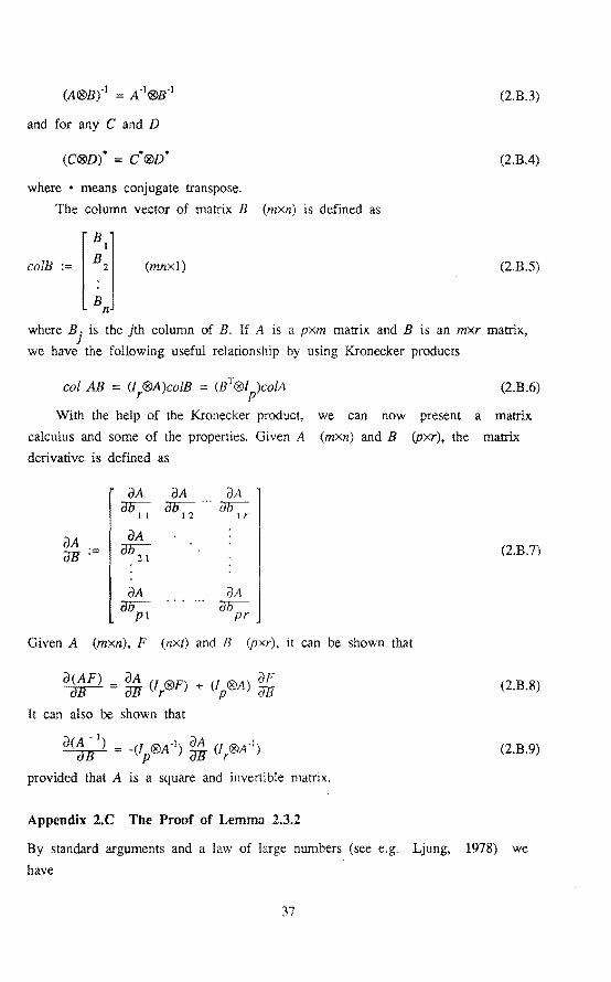
Appendix 2.C The Proof of Lemma 2.3.2

(2.B.7)

(2.B.8)

(2.B.9)

By standard arguments and a law of large nnmbers (see e.g. Ljung, 1978) we

have

37

Vj:j.fJ,Ö) -t l im EVj:;((),Ö) as N -t oo

N-t<X> (2.C.l)

w.p. 1 and uniformly in e e D,( After some ealeularion, we have

11 1 N T 1 N ,· V N(fJ,B) = BId + N I 'Jf(t,e)·'Jf (t,e) + N I 'Jf (t,e)(l d®r(t,e)) (2.C.2)

t=l t=l

where 'Jf'(t,e) (dxdp) is the seeond derivative matrix of ;(tIe). Combining

(2.C.2), (2.3.57) and (2.3.59) gives

Vj:J.~~.B)-7 BI+E'Jf(t,a· (n))'Jf,.(t,e· (n)) + E'Jf'(t,e· (n))[/ d®r(t,a· (n))]

(2.C.3)

using the faet that ~(t) and 'Jf'(t,e) are independent.

Remark The reason why 'Jf(t,e) and 'Jf'(t,e) are independent of e(t) is due to

the faet that the "predietion error" criterion is used: ;(tI fJ) is dependent

only on the previous y and u, i.e. ;(tI ()) is only dependent on the previous

~. and ~(t) is an independent variable, therefore ;(tI fJ)and ~(t) are

independent, this implies that 'Jf(t,e) and 'Jf'(t,8) are also independent of

~(t). •

It remains to be shown that the operator norm of the last term of (2.C.3)

tends to zero as n tends to infinity. We note that E.''Jf'(r,e·(n))-r(t,e·(n)) is

a symmetrie matrix and for the (kJ) entry of the matrix, using (2.3.60)

/ E{rr(t,e·(n))·r(t,e·(n))}E{;eke.<tlfJ) ;eke.<tje)} ::;; een In (2.C.4) .I J

since the predietor filter and their seeond derivatives are stable. Henee

d A

I iE y~ e<tifJ)-r(t,e'(n))j::;; see k= 1 kj n

(2.C.5)

Now, the operator norm of any symmetrie matrix is bounded by its absolute

row sums. Henee we have

IIE'Jf'(r,e*(n))[/d®r(t,e*(n))]n ... 0 as n ... oo (2.C.6)

In view of the definition (2.3.44) and (2.C.6) we obtain (2.3.61). IJ

3!1

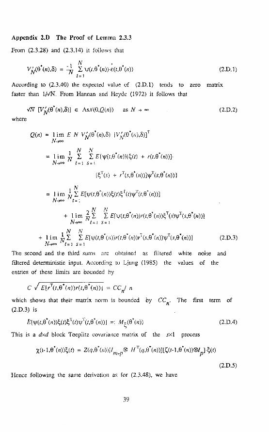
Appendix 2.D The Proof of Lemma 2.3.3

From (2.3.28) and (2.3.14) it follows that

• -1 N • • • Vj.y(9 (n),S) = -"N L \jl(t,e (n))·E(t,e (n))

t= l (2.D.l)

According to (2.3.40) the expected value of (2.D.l) tends to zero matrix

faster than 1/VN. From Hannan and Heyde (1972) it follows that

IN [VN(e\n),S)] e AsN(O,Q(n)) as N -. oo (2.D.2)

where

Q(n) = 1 im E N VN(e*(n),S) [VN(e\n),o){ N-.=

. 1 N N * * = ltm N L L E[\jl(t,e (n))IÇ(t) + r(t,e (n))}

N-.= t=l S=l

T T • T * [Ç (s) + r (s,e (n))]\jl (s,e (n))}

N I im ~ L E[\jl(r,e*cn))Ç(t)ÇT(t)\j/T(t,e\n))] N-.oo t= I

. 2N N • • T T • + l1m N L L E[\jf(t,e (n))r(t,e (n))Ç (s)\jl (s,e (n))]

N-.= t=l S=l

N N 1 · * * T* T• + 1 i m N L L E[\jf(t,e (n))r(t,e (n))r (s,e (n))\jl (s,e (n))] N->""" t=l s 1

(2.D.3)

The second and the third sums are obtained as filtered white noise and

filtered deterministic input. According to Ljung (1985) the values of the

entties of these limits are bounded by

.; T • • c E[r (t,e (n))r(t,e (n))l

which shows that their matrix norm is bounded by CC r( The first term of

(2.D.3) is

E[\jf(t,e· (n))Ç(t)Ç T(t)\j/T(r,e* (n))] =: M ç (8\n)) (2.D.4)

This is a dxd block Toeplitz covariance matrix of the sx1 process

X(t-1,9* (n))Ç(t) = Z(q,e* (n))l/ m+p ® rr'~'(q,e* (n))][Ç(t-I,e• (n))®/p)-Ç(t)

(2.D.5)

Hence following the same derivation as for (2.3.48), we have

39

lim ~ Wn(ro)M;(9\n))W~(-ro) n~

(2.0.6)

and the lemma is proved. t:l

40

Chapter Three

IDENTIFYING THE NOMINAL MODEL AND THE ERROR BOUNDS

3.1 Introduetion

In reality, all models are subject to errors. Hence when using a model,

attention must be paid to the consequences of the modeHing errors. When

identification techniques are used to obtain a mathematica! model of a

dynamica! process, the modeHing errors (model uncertainty) are caused by the

process disturbances, measurement noises, constrained model setand round off

errors of the computer.

In recent years, a so called robust control theory has been developed

which studies the problem of control system analysis and the design in face

of process (plant) modelling errors; cf. Zames (1981), Doyle and Stein

(1981), Vidyasagar (1985) and Kouvaritakis and Latchman (1985a, b). In order

to apply the theory one needs not only a nomina! model of the process, but

also a suitable description of the modelling en·ors, namely an upper bound of

the process transfer function errors.

So far techniques to produce both the model and the error bound, however,

have received re1atively little attention in the control community. Cloud and

Kouvaritakis (1986) proposed an upper bound matrix for the MIMO black-box

finite-impulse-response models, where process output disturbances are assumed

to be white noises. Kosut (1986) derived an upper bound for SISO prediction

error models in the case of an open loop experiment.

Based on the asymptotic theory developed in Chapter 2, algorithms for

calculating black-box models logether with an upper bound of model errors

will be proposed in this chapter. Many techniques should be combined to reach

this goal, but the work here wil! concentrale on the denvation of the upper

bound matrix of MIMO transfer functions. Because of the stochastkal nature

of the theory developed, it is not surprising that a probability bound will

be defined and estimated. Four algorîthms will be given which fit different

kind of applications; the first two are based on non parametrical

identification and the latter two are based on the parametrical

identification. Two numerical tests are used to illustrate the theory.

41

3.2 Algorithms by Speetral Analysis

Based on the asymptotic theory, there are several possibilities for

estimating a bound of the modeling errors. Remember that the results of

speetral analysis given in the last chapter hold only for experimental data

obtained on .a process in open loop; this implies . that the algorithms given in

this section will not work for closed loop data.

3.2.1 Some Practical Aspects of Speetral Analysis Metbod

Before giving the algorithms, some discussion on how to determine the maximum

time lags for speetral analysis is presented bere; because this question is

not yet answered clearly in the identification literature. We will show the

idea in the SISO case. The conventional metbod as described in

(2.2.1)-(2.2.3) uses the same n for calculating <P~(ro) and <P~y<ro); thus the

symmetrical Fourier transform is used for the calculation of <P~y<ro). It will

be shown here that this is not proper for estimating the process transfer

function. A modified estimation method wil! be proposed.

Asymmetrical Windowing

In the last chapter we have seen that the "order" (2n+l) should be chosen as

small as possible to keep the varianee of the estimate small (see (2.2.8));

on the other hand, n should be large enough for unbiased estimation. In fact,

the maximum time lags of R uy<'t) can be determined from the physical knowledge

about the process and the input signa!.

Assume that the process impulse response is finite, with length Ti the

maximum time lag of the input auto-correlation function R u<t) is tu. Then it

is obvious that the maximum time lags of cross-correlation function Ruy(t)

are asymmetrical to the zero-axis, that is,

(3.2.1)

We see that for processes with finite impulse responses, one can use an

input signa! with tu as smal! as possible, and modify the estimation (2.2.2)

as follows:

42

} -lt s; co s; 1t (3.2.2)

Notice the difference in the summatien intervals. The way to calculate <P~y<co) can be seen as using an asymmetrical rectangular window; the physical

knowledge of the process and the input which is often available is used here.

Then from Theerem 2.2.1 it can be shown that we now have

~ -~ 2'C + 'C +1 (Ï) (CO) var[ G-d/ ;] a. u N g · ~ (3.2.3)

u Of course, in general and theoretically, the length of {g

0(k)} is infinite.

But it is well known that one can always truncate a stabie impulse response

with a sufficiently small error. Hence one can take 'Cg to be the practical

length of the process impulse response which can be determined, e.g., by

observing the step response of the process.

Not only can we determine 'C11

easily, but also manipulate it because we

often have the freedom of input design (This problem will be discussed in

Chapter 6).

The asymmetrical window proposed here can be used together with normal

lag windows, such as Bartlett, Tukey or Hamming window, in order to further

reduce the varianee further. Then (3.2.2) becomes

'Cu +'Cg

~Y(co) = 'L 'C - 'C u

} -lt s; co s; 1t

R~Y ( 'C)w(t)e- itco

(3.2.4)

where w('C) denotes the lag window. The effect of these lag windows is

smoothing , so considerable bias of the estimate can be introduced in the

frequency range where the process transfer function changes rapidly (see

Jenkins and Watts, 1968). Therefore, normal lag windows should be used with

caution.

43

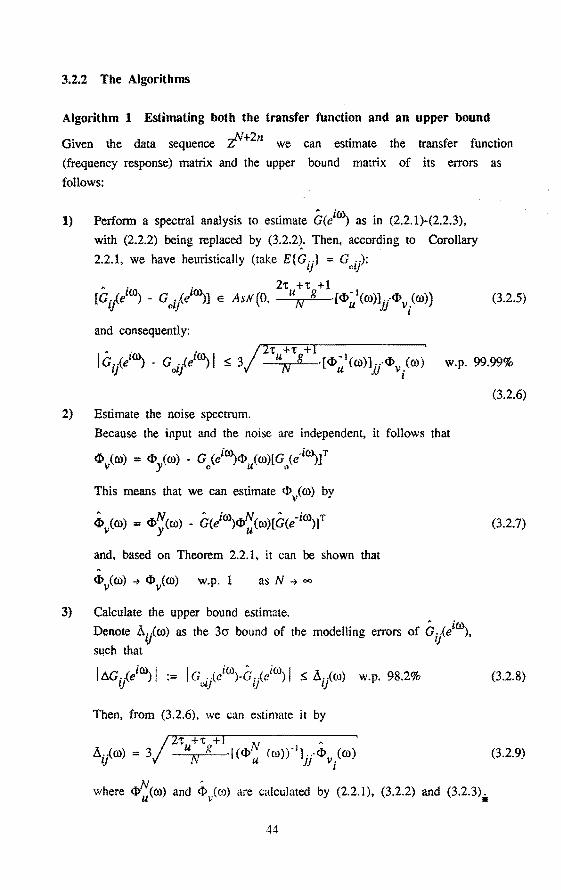
3.2.2 The Algorithms

Algorithm 1 Estimating both the transfer function and an upper bound

Given the data sequence z!'+2n we can estimate the transfer function

(frequency response) matrix and the upper bound matrix of its errors as

follows:

1) Perform a speetral analysis to estimate G(i~ as in (2.2.1)-(2.2.3),

with (2.2.2) being replaced by (3.2.2~. Then, according to Corollary

2.2.1, we have heuristically (take E{Gij} = Gei/

A • • 2t +t +1 [GÎJ.(e

100) - Goi/e'~] e AsN(O, llN g ·[<l>~ 1 (ro)]j/<l>v.<ro))

I

and consequently:

(3.2.5)

w.p. 99.99%

2) Estimate the noise spectrum.

3)

Because the input and the noise are independent, it follows that

<l> (ro) = <l> (ro) - G (i~<l> (ro)[G (e·îro)JT V y o U o

This means that we can estimate <l> v(ro) by

cÎ>v{ro) = <l>~(ro) - G(i~<l>~(ro)[G(e·i~]T

and, based on Theorem 2.2.1, it can be shown that

as N -+ oo

Calculate the upper bound estimate.

Denote lJ.i/ro) as the 3cr bound of the modelling errors of Gy<i~. sqch that

I iro 1 . 1 iro A iro 1 x t:J.G .. (e ) .= G .. (e )-G .. (e ) ::::: L,l .. (ro) w.p. 98.2%

Ij olj l) lj

Then, from (3.2.6), we can estimate it by

/

2t +'t +l A

JJ.i/ro) = 3 u N g ·l(<l>~ (ro)r1Jj/<l>v/ro)

N , where <l> u(ro) and <l> v(û>) are calculated by (2.2.1), (3.2.2) and (3.2.3)•

44

(3.2.6)

(3.2.7)

(3.2.8)

(3.2.9)

Remarks:

Notice that the probability of 3cr bound for a complex random variabie with

normal distribution is higher than that of a real random variable.

It is clear that the maximum time lag for calculating ~(oo) is ('tu +tg>Other windowing techniques can be used to improve the spectrum estimation. If

the windowing technique is used properly, the MSE of the estimates will be

smaller than that given in Theorem 2.2.1. This means that the relation in

(3.2.8) will hold with a higher probability. But caution must be paid in

order not to introduce too much bias.

Algorithm 2 - Estimating the upper bound for a given nomina! model

Speetral analysis is a nonparametrieal method for transfer funetion

estimation. For many applieations, parametrie roodels are used. Sueh roodels

can be obtained by parametrie identification, sueh as prediction error method

(Ljung, 1987; Söderström and Stoica, 1989), or derived from the first

principles (mathematica! modelling). If the model is too complex to be used,

model reduction techniques can be used to obtain a simplified model; see

Oiover (1984). Denote ê}(e10)) as the transfer function matrix of the

parametrie model of the process, where l means "low order". Then, based on 'I . -N+2 G (e'00

) and a properly generated input-output data sequence :c · n, öne can 'l .

estimate an upper bound of the error of G (e1~ as follows:

1) Calculate the output residual from the model,

(3.2.10)

or

' -1 e(t) = b.G(q )u(t) + v(r) (3.2.11)

where

b.G(q-1) = G (q-t) _ (;f(q-t) 0

(3.2.12)

45

where <!>NA (ro) is calculated as in (2.2.1) and (3.2.2) by replacing u ei

yp) by ei(t).

We note that (3.2.11) is a MIMO process with u(t) being the input,

e(t) the output and v(t) the disturbance. Therefore, Theorem 2.2.1

can be applied to the estimate (3.2.12). Then, according to Corollary

2.2.1, we have

A ' 0 2't +'t + 1 [t:.Gij(i~ - t:.Gij(e

100)] e AsH(O, uN g [<!>~1 (ro)]j/<l>v.<ro))

l

and

(3.2.13)

w.p. 99.99%

(3.2.14)

3) Estimate the noise spectrum.

Following the same reasoning as for (3.2.7) we can have an estimate

of <!> y<ro) by

eb (ro) = <l>'f(ro) - ÛJ(ei~ <l>N(ro) ÛJT(e·i~ (3.2.15) v e u

4) Calculate the estimate of the bound.

t:.G.t..i00) = [Û;.~ei~] + fb.G .. (i~ - Ûl .. (i~J lj lj lj lJ

We eaU the first term the bias part and the second term the varianee

part of the modeHing errors t:.Gij(ei~. Then

it:.Gi/i~l :::: !t:.Gi/i~l + !t:.Gij(i00)- t:.Gij(i

00>1

From (3.2.14) we have

(3.2.16)

where t:.a.~i~ is obtained from (3.2.12) and $ (ro) is determined by lJ ~

(3.2.15).

Now, if we denote ~ .. (ro) as an upper bound of the modelling error . Ij

I ÄG;/e'~ I, we have

46

(3.2.17)

Numerical Test 1

In order to illusttate the theory developed here, a numerical test is

performed under the condition that the real process is known exactly,

although that is not ttue in practice. An estimated finite impulse response

(Markov parameters) of the 2 input and 2 output glass tube process (See

Example 1.1) is used as the real process. The length of the Markov parameters

sequence is 50.

The input/output data sequence is generated by simulating this model with

inputs u and disturbances v being both white noises. The data length is

N=!OOO; the signa! (power) to noise (power) ratios at both outputs are about

•

10 dB. The low order nomina! model is obtained by an output error estimation

method using the data sequence. The model is paramettized as a mattix

fraction description (MFD) model, with both row degrees being 2:

(3.2.18)

where

A(q) B(q)

and aii(q), bi/q), iJ = 1,2, are polynomials of q, with degree 2. This

model sttucture is called diagonal form MFD.

Fig. 3.2.1 shows the real impulse responses and those of the low order

model. When the I/0 data of the process (the Markov parameters) and the low

order model are available, Algorithm 2 can used to estimate the upper bound

mattix .ó.(ro) of the modelling errors. Here n is taken to be 100; and the

symetrical Tukey window (i.e., normal window technique) is used for the

speetturn estimation. Fig.3.2.2 gives the real rnadelling error and the

estimated upper bound in the frequency domain. This result confirms our

theory and also shows that the 3cr bound is not very tight.

47

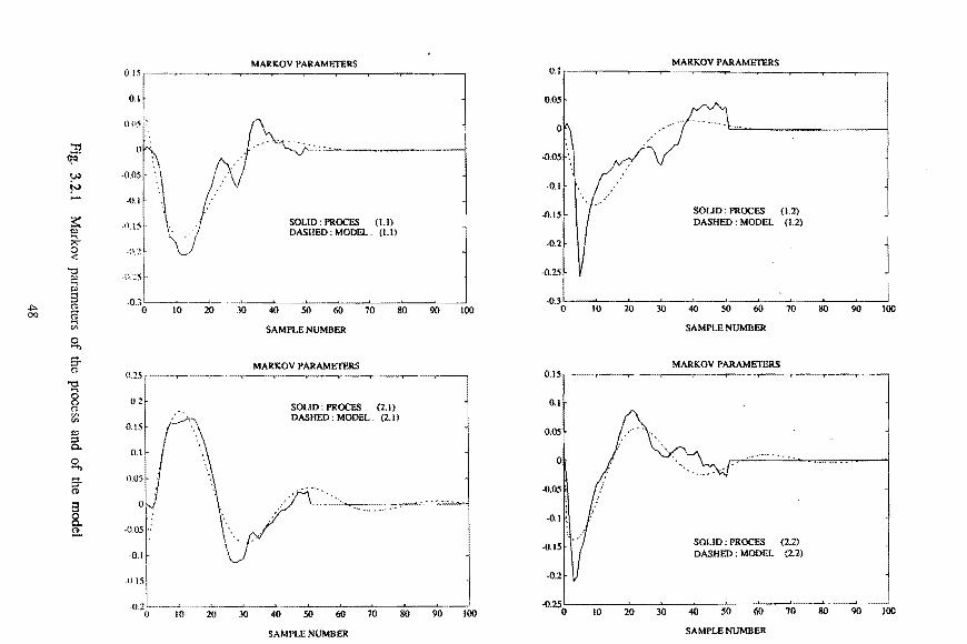
MARKOV PARAMETERS MARKOV PARAMETERS 0.1

0.05

0

::n ~ ·ll.OS ·,

!.>l

!v -0.1 - ·0.1

~ -0.15 SOUD: PROCES (1,2)

-0.15

~-SOLID : PROCES (1.1) DASHED : MODEL (1,2)

El DASBED: MODEL. (1.1)

j ;.;- -0.~ l -0.2 0 <

"0 o::sl -0.25 El "" a ~0.3 ~---'----~~. ' ' ·0.3

-"" (1) 0 10 20 30 40 50 60 70 80 90 100 0 10 20 30 40 50 60 70 80 90 100 00 ~

VI SAMPLE NUMBER SAMPLE NUMBER

0 ....., Er MARKOV PARAMETERS MARKOV PARAMETERS (1)

0.25 --~---yo--·----r-- 0.15 "0 .... g 0,2

SOUD: PROCES 0.1 (1) (2.1) VI DASHED : MODEL (2.1) VI

IX> 0.05 :::;, p..

0 0 ....., Er -0.05 (1)

a &

-005 ':: a -0.15 SOLID: PROCES {2.2)

-0.1 DASHED : MODEL (2.2)

-Olt -0.2

·0,2 ~--~~----1-----4-----l. ·0.25 () 10 20 30 40 50 60 70 80 90 100 0 10 20 30 40 50 60 70 80 90 100

SAMPLE NUMBER SAMPLE NUMBER

:!! q<l

VJ tv tv

s:: 8. ~

..,.. s· \0 (Jq

(\)

::j 0 ... "' § Q.

.... ::r 0

t:: '1::) '1::)

~ er g ::; Q.

"'

3 SIG).!A UPPER BOUND

SOLID: MODEL ERROR (Ll)

DASliED: UPPER BOUND (Ll)

'\;

FREQUENCY (radls)

3 SIGMA liPPER BOUND

SOLID: MODEL ERROR (2.1)

DASHED: UPPER BOUND (2.1)

!'•

'• -,;, ,-,- '·• ,, '"

FREQUENCY (rad/s)

3 SIGMA UPPER BOUND

'• ., '•

·-: SOLID : MODEL ERROR ( 1.2)

DASliED: UPPER BOUND (1.2)

;" '''

j 0.5 L5

FREQlJENCY (radis)

3 SIGMA UPPER BOUND 1.6

1.4

1.2

SOLID: MODEL ERROR (2.2)

0.8' DASHED : UPPER BOUND (2.2)

'.'

0.6

::r~~ l 0 --~-~-- . . - --~-----L-----------__)

3.5 0 0.5 1.5 2 2.5 3.5

FREQlJENCY (ratVs)

3.3 Algorithms by Prediction Error Method

3.3.1 Two Simple Model Structures

ARX-Model (equation error model) One of the simplest parametrical · model

structures for the model (2.1.1) and (2. 1.5) is

A(q)y(t) = B(q)u(t) + e(t) (3.3.1)

where A(q) and B(q) are polynomial matrices:

A(q) = I + A q-1 + ··· +A q·n } p 1 n

B(q) = B q·1+ ··· + B q-n 1 n

(3.3.2)

where n is called the order of the model. Note that this n is different from

the n in speetral analysis; typically, for identifying the same process a

much lower model order can be used for paran1etrical models.

Comparing to the general model this gives

G(q) = A'1(q)B(q), H(q) = A"1(q)

Since the white noise e(t) enters equation (3.3.1) directly, this model is

often called equation error model. The parameter vector is

9(n) = col[A1

B2

... An Bn]

and the dimension of 9 is

d = n(p2 + pm)

Applying (3.3.1) to calculate the prediction error, we get from (2.3.3)

(3.3.3)

(3.3.4)

e(t) = A(q,9)y(t) + B(q,O)u(t) (3.3.5)

Because the error e(t) is linear in the model parameters in (3.3.5), there is

an analytica! solution for the parameter estimation when the quadratic loss

function (2.3.4) is used. This is the most important advantage of the

equation error method. But if the real equation error is not white noise, the

estimates with a low order model will be biased, which is the disadvantage of

the method.

FIR (finite impulse response) Model When talcing

A(q) =lp

(3.3.1) becomes

50

y(t) = B(q)u(t) + e(t) (3.3.6)

This is the FIR model. It has the same advantage as ARX model has. The

disadvantages are: (1) in practiceone needs to take a very high order n in

(3.3.6) in order to model the process dynamics; (2) this model set in general

will not give consistent estimation of the process transfer functions for the

closed loop experiment data, because the model of the disturbance is fixed to

identity which is too simple; cf. Gustavsson et al. (1977).

3.3.2 The Nomina! Model and the Upper Bound Matrix

In this section, we propose two algorithms for the estimation of the nomina!

process model and an upper bound matrix of the model uncertainty. Because the

theory in the previous chapter is asymptotic both in the number of data N and

the model order n, the results wil! be more adequate when the number of data

is large and the model order is high. But in practice low order models are

used for simulation, predietien and controller design. So our approach is to

start with the estimation of a high order model and then apply model

reduction techniques to arrive at low order models.

This approach bas its practical background. For industrial process

identification and control, we can have a large amount of data. For unstable

or nearly unstable processes, a scheme is proposed for increasing the

experiment time in Zhu et al. ( 1988) and Chapter 5 of this thesis. Sometimes

we have to use high order models to fit the complex dynamics of the process.

One can avoid numerical problems when combining high order estimation and

model reduction; cf. Backx (1987) and Wahlberg (1985).

In order to present the idea more clearly, let us assume in this section

that the process is operating in open loop; the closed loop experiment case

can be treated along the same line as in Algorithm 4.

Algorithm 3

The asymptotic theory implies that the model structure is not important for

high order models. Hence if we are only interested to identify the process

dynamics, the FIR model can be used as fellows:

1) Estimate the parameters of the FIR model with the order n sufficiently

large, e.g., n 50-100. In practice n wil! have to be determined

according to the engineering knowledge about the process.

51

2) Calculate G~i'))) as in (2.1.4) when replacing g(k) by Bk. Then

according to Theorem 2.3.1 and (2.3.79), we have heuristically

iro. A n iro ) ( n . 1 ) { G . . (e J - G. ~e ) e AsN 0, •~[4> (ro)] .. ·4> (ro) ol} Ij IV U }} V j

IGoi}i~- G7/i00)1 s 3/N-r<~>~1 (ro)]jf<l>v.<ro)' w.p. 99.99% l

where [<1>~1 (ro)]jj is the (jJ) element of <1>~ 1 (ro), and v.(ro) is the l

(i,i) element of v< ro).

(3.3.7)

(3.3.8)

3) ~erf<?rm a model rednetion on G~(i~ to obtain a low order model

d(e1~. where I denotes the /ow order. Two well known techniques of

model rednetion are the method of trucated balanced realization and

the method of Hankel norm approximation; cf. Glover (1984).

4) Define the modelling errors as

.. iro G iro. GA 1 iro l.J. •• (e ) = .. (e J - .~e )

lj olj lj "diJ (3.3.9)

where oiii~ is the {iJ) element of o~<i~. Then

(3.3.10)

The first term in (2.3.10) we call the bias part of the modelling

errors, and second term the random (variance) part of the modelling

errors. Now

(3.3.11)

From (2.3.8) it follows that

IA.~i~ I s I g~ .(eiro) - lei~ I + 3/N~ [ <l>u.1(ro)]11i'<l>v .<ro)' lj lj. Ij J l

(3.3.12)

This is the basis for estimating the upper bound matrix.

5) Define the upper bound matrix

52

&(ro) = (A .. (ro)} Ij

(3.3.13)

such that

I fli/iro) I s: Ai/ro) 'diJ 'dro (3.3.14)

Then we can estimate A(ro) by

' Here d>u(ro) and <l>v(ro) are the estimates of <l>u(ro) and <t>v<ro)

respectively, which can be calculated by

, 'tu N <l>u(ro) = I. [& I. u(t)uT(t-'t)] -i rot e (3.3.16)

't'=·'t tI u

'tu+n 1 N, 'T

 v(ro) = I. [IV I. e(t)e (t-'t)] e-iro't (3.3.17) 't"'. 't -n t u

where e(t) is the output residuals of the estimated FIR model:

;(t) = y(t) - G~q)u(t) (3.3.18)

• Remarks

It can be shown that

as N -? ""• n -? "" (3.3.19)

based on Corollary 2.3.1 and the large number theorem.

In practice (3.3.16) and (3.3.17) can be modified by using windowing

techniques in order to improve the spectrum estimation as mentioned before.

In formula (3.3.15) we find that the bias part of the modelling errors is

determined by model reduction; the random part can be affected by the input

spectrum, the model order and the number of data, which are design variables

chosen by the user. If the modeHing errors are too big at some frequencies

for a specific use of the model, we know from (3.3.15) that we can reduce the

modelling errors at those frequencies by: (1) performing another model

reduction, (2) modifying the input spectrum, (3) using more data, and (4)

reducing the the model order of the high order model. The first choice will

influence the bias part of the modelling errors and the latter three chokes

will influence the varianee part of the modeHing errors. The last choice

53

should be made with caution, because too low an order will introduce more

bias.

This algorithm can not work for closed loop data, because the

disturbance model is fixed to be the identity. •

Numerical Test 2

A numerical test is performed for Algorithm 3 by using the sarne FIR model of

Numerical Test 1. This is a process with 2 inputs and 2 outputs. The order of

the FIR model n is 50; again we will consicter this model to be the real

process.

First a simulation is performed to generate input/output data, where both

the inputs and the output disturbances are white noise signals. The signa! to

noise ratios at outputs are about 10 dB. Then a 50th order FIR model is

estimated by using 1000 samples from the IlO data from the simulation. The

FIR parameters of the process and of the estimated model are shown in Fig.

3.3.1.

From (3.3.12) it is clear that only the 3o bounds of the random part of

the errors need to be checked for validating (3.3.15). The 3o bounds and the

errors of the FIR model are shown in Fig. 3.3.2, where harnming window is used

for the estimation of input and disturbance spectra. Again we find that 3o

bounds are loose, and 2o bounds (w.p.98.17%) are good enough for the testing

exarnple. More information about these numerical tests can be found in van

Beuningen (1988).

Algorithm 4

If we want to estimate the disturbance model as well, an ARX model structure

can be used with a high order, e.g. n = 20 - 30. The idea is similar to

Algorithm 3, and the following steps are proposed:

1) Estimate the parameters of the ARX model. Then we have

(3.3.20)

and the spectrum estimates of the disturbances are

<Î>v(ro) = ANt(eiro)R Af/(e·i~ (3.3.21)

where R is the estimated covariance of the prediction residuals.

54

0.1 0.1

0.05

-0.1

-0.3 50 0 50

Samples Samples

Fig. 3.3.1 Markov parameters of the process (solid)

and of the FIR model (dashed)

0.1

o.o5 N\.rét.\~.N\..iW: " 0: ~ff -~ ~ :: ~"'\.

0 I 2 3 4 0 2 4

·:~Rç·· ! :~ :·~

0.05~-\./(/J \J.j \t;:;:f\ ol ' · '' 1 • , I

''~" 0.15

0.1 ' ~

0.05 r~: n ,•, " ;: ;. ·~ "f\ i1

l .. ~ v .v1k) \fV'·.i ·' 0 - ~ • " 'f ·~

0 I 2 3 4 0 1 2 3 4

Frequency (rad./sec.) Frequency (rad,fsec.)

Fig. 3.3.2 Errors of the FIR model (dashed) and 3o bounds (solid)

55

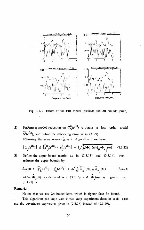
0,15, Error and 2sig'1'a bOltnd (2.1)

Fig. 3.3.3 Errors of the FIR model (dashed) and 2a bounds (solid)

2) Perform a model reduction on G~(i~ to obtain a low order model

ê1ci0\ and define the modeHing error as in (3.3.9)

Following the same reasonin'g as in Algorithm 3 we have

1 i~ 1 1 ~ n iro A I iro 1 /n . 1 • !i;fe s; g de ) - gi/e ) + 2 IV[ u (ro)]j/ v /ro) (3.3.22)

3) Define the upper bound matrix as in (3.3.13) and (3.3.14), then

estimate the upper bounds by

h.ï/ro) = Jg7fi00) - g~fei00) I + 2/ ~r<Î>;/<ro)]j/«Î>v /ro)' (3.3.23)

where <l>u(ro) is calculated as in (3.3.16), and <l>v(ro) is given in

(3.3.21) .•

Remarks

Notice that we use 2a bound here, which is tighter than 3a bound.

This algorithm can cope with closed loop experiment data; in such case,

use the covariance expression given in (2.3.78) instead of (2.3.79).

56

3.4 Conclusions

Based on the newly developed asymptotic theory on MIMO transfer function

estimates, a method for identifying a nomina! model of a MIMO process,

together with an upper bound matrix of the modelling errors in the frequency

domain has been proposed. Four algorithms have been given. The first two

algorithms are based on the properties of speetral analysis, which can not

work for closed loop experiment data. Note that Algorithm 2 can calculate an

upper bound matrix for an existing model which neects not to be a black-box

model. The last two algorithms are based on the properties of parametrical

methods; the ARX and FIR model structure are proposed because they are simple

to compute. The numerical tests have shown the adequacy of the method. The

next chapter will show that the upper bound matrix can be readily used for

robust stability analysis and design of a feedback control system. It will be

shown in Chapter 6 that the result of our method not only supplies useful

information for checking the robustness of a feedback control system, but it

also suggests clearly the ways for remodelling and re-design if the model

and/or the controller cannot pass the test. This is specially useful for

engineering applications of identification and control theory. The upper

bound matrix also provides a new way of model validation.

57

Chapter Four

ROBUST ST ABILITY OF MIMO LINEAR FEEDBACK SYSTEMS

4.1 Introduetion

This chapter presents a study of robust stability analysis. This part of the

work is not original, but it is needed for combining identification and

robust controL

One of the basic approaches for robustness analysis of MIMO systems is

the singular value analysis (Doyle and Stein, 1981). This metbod describes

the process by a nomina! model and a perturbation (model uncertainty) which

is norm-bounded. Here the model uncertainty is described by a scalar, hence

it is called unstructured model uncertainty, meaning that in the description

the matrix structure of the uncertainty is lacking. This method is

mathematically simple, but it can not use the structural information about

model uncertainty which is often available in practice, and thus may lead to

a conservative interpretation of robustness.

One way of representing structured model uncertainty of MIMO processes is

that the matrix additive model error is bounded by an upper bound matrix A((l))

as derived in the previous chapter. Several researchers have studied the

problem of robust stability for systems subject to the structured model

uncertainty. Owens and Chotai (1984) and Lunze (1984) proposed to use the

speetral radius technique for assessing the stability, which is based on the

properties of positive matrices. But their method is not necessarily better

than the singular value analysis, in the sense that the method can give more

conservative results than the singular value method, and vice versa.

Kouvaritakis and Latchman (1985a,b) developed a method for robust stability

analysis, which uses a non-similarity sealing technique. Their result is less

conservative than the last two methods.

In Section 4.2, these methods for robust stability analysis will be

introduced and compared; in Section 4.3, the robust stability of internal

model control scheme is discussed. In Section 4.4 a procedure for combining

identification and robust control is proposed. Section 4.5 gives conclusions.

58

4.2 Robust Stability Analysis

Assume a controller C has been designed for some puryoses, e.g., senstUvtty

reduction, inpu! tracking, based on the process model G, so that C must at

least stabilize G. But this is not enough, C must stabilize the real process

P, which is not completely known. By robust stability analysis we mean

checking whether this condition is fulfilled.

4.2.1 The Class of Perturbations

Followi~g the ideas in the previous chapter, the process is described by the

model G(q) and the upper bound matrix f.(w), such that ~

G (q) = G(q) + L1(q) 0

I L1ij(eiw) I :::; t.i/W) "i iJ "i(() }

where G (q) is the true causal transfer operator of the process, which is 0 ~

real rational; G(q) is the nomina! model of G (q), real rational and proper; A 0

(4.2.1)

G (q) and G(q) are both stable; hence L1(q), the unknown perturbation matrix, 0

is also real rational and stable; and f.(w) is the bound matrix; its entries

take real positive values which are functions of the frequency w; they need

not be rational.

The description of model uncertainty in (4.2.1) is called structured

perturbation, in the sense that it preserves the multivariable nature of the

problem: the amplitude of the error of each transfer function is bounded by

the entries of t.{w) in the frequency domain.

An earlier description of the model uncertainty (see, e.g., Doyle and

Stein, 1981) is given by an upper bound on its maximum singular value (norm),

a(L1(wiw)). This class of model uncenainty is called unstructured

perturbation, because the bound is a scalar, and cannot use any knowledge

about the structure of L1(i~. One might ask what is the relation between the

unstructured uncertainty and structured one given in (4.2.1). It can be shown

(Kouvaritakis and Latchman, 1985a, Zhu 1987).

a(L1(ei<O)) :::; a(L1 +(ei00)) ::; a(Ó{<O)) (4.2.2)

where L1+ := { IL1 .. 1 ). This means that if t.{w) is known, one can calculate from V . it a bound for the maximum singular value of L1(e'~.

Denote the structured class of perturbations from ( 4.2.1) as:

D • := { L1(eiw): I L1;li00) I s f.i} w)

and the class of unstructured perturbations

59

"i iJ "i(() J (4.2.3)

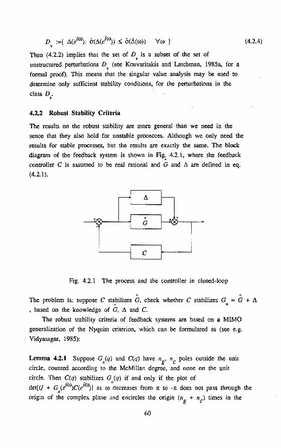
Then ( 4.2.2) implies that the set of D is a subset of the set of $

unstructured perturbations D (see Kouvaritakis and Latchman, 1985a, for a u

formal proot). This means that the singular value analysis may be used to

determine only sufficient stability conditions, for the perturbations in Jhe

class D . •

4.2.2 Robust Stability Criteria

The results on the robust stahility are more general than we need in the

sence that they also hold for unstable procecces. Although we only need the

results for stabie processes, but the results are exactly the same. The block

diagram of the feedback system is shown in Fig: 4.2.1, where the feedback

controller C is assumed to be real rationat and G and A are defined in eq.

(4.2.1).

..

Fig. 4.2.1 The process and the controller in closed-loop

A A

(4.2.4)

The problem is: suppose C stahilizes G, check whether C stahilizes G == G + A A 0

, based on the knowledge of G, A and C.

The robust stahility criteria of feedback systems are based on a MIMO

generalization of the Nyquist criterion, which can be formulated as (see e.g.

Vidyasagar, 1985):

Lemma 4.2.1 Suppose G0(q) and C(q) have ng, nc poles outside the unit

circle, counted according to the McMillan degree, and none on the unit

circle. Then C(q) stahilizes G (q) if and only if the plot of

det[(/ + G (iO)c(iro)] as ro 0

decreases from 1t to ·1t does not pass through the 0

origin of the complex plane and encircles the origin (ng + nc) times in the

60

clockwise sense.

It is obvious that we cannot use this criterion to test the stability of

the system in Fig. 4.2.1, because in eq. (4.2.1) G is not exactly known. 0

What we can check is the number of encirclements (n.o.e.) of

•

According to our assumption, G(s)C(s) and G (s)C(s) have the same number of 0

unstable poles. Hence the system is robustly stable if and only if

(n.o.e.det[/ + (G + .1)C] = n.o.~.det[I + GC] V'ó.eD,}. ~

This is assured if and ~only if det[I+(G+ó.)C] remains non-zero as G is warped

continuously towards (G+-1), i.e.

det[I + (G + EA)C] :;; 0 V'ee [0, 1] V'ro V' MD

But

det[(/+(G+EA)C]

det[ (I +GC)+eó.C]

= det[I + GC]·det[l + EAC(/ + GC)-1]

Because C stahilizes G, we have

det[I+GC] -:~: 0 V'ro

Thus (4.2.5) is assured if and only if

det[I + e.1C(/ + GC)'1] -:~: 0 V'ee [0,1] V'ro V'ó.eD

Denote p(A) as the speetral radius of matrix A:

p(A):= max I A/A) I and \(A) is the i-th eigenvalue of A. Then we have

lemma 4.2.2 The system in Fig. 4.2.1 is stable if

p[.1C(/+GCf1J < 1 V'ro V'ó.eD

proof. Suppose that

det[I + EAC(/+GC)'1] = 0 for some ro, .1 and e

then -1 is an eigenvalue of eó.C(/+GC)-1• But

p[EAC(I + êcr'1 $ p[.1C(I + êcr'1 and hence

p[.1C(I + êcr'J ~ 1

61

V'ee [0, 1]

(4.2.5)

(4.2.6)

(4.2.7)

•

This contradiets (4.2.7).

Again, this can not be used directly, because we only know the upper

bound matrix à. But (4.2.7) is the starting point for deriving other

applicable stability criteria.

0

We know that the speetral radius of a matrix is bounded by its maximum

singular value (Doyle and Stein, 1981). Then for each ro

p[äC(/ + GC)"1] s; á[8C(! + GC)"1

])'1]

s; á(ä)á[C(/ + GCr11

:::; á(à)á[C(/ + GC)"1]

Denote T := C(/ + GC)'1, we get the singular value analysis criterion (see

Vydiasagar, 1985, Doyle and Stein, 1981):

Tbeorem 4.2.1-singular value metbod The system in Fig.4.2.1 is stabie if

á(à)á(T) < 1

As discussed before, this criterion does not use the structural

information of à, it only gives a sufficient stability condition for the

class of (4.2.1) and it can be conservative. The advantage of this metbod is

its numerical simplicity and reliability. Therefore it can be used as a rough

assessment of the stability.

(4.2.8)

The bound matrix 6 is a positive matrix, which means that the entries of

6 are all real and positive numbers. So one can think of using the theory of

non-negative matrices for a robust stability test. From this theory (Berman

and Plemmons, 1979), we have

Thus, (4.2.7) and (4.2.9) give another stability condition (ûwens and Chotai,

1984; Lunze, 1984), which is called speetral radius method:

(4.2.9)

Tbeorem 4.2.2-spectral radius metbod The system in Fig.4.2.1 is stabie if

p(6T') < 1

This metbod uses the structural information of à, but it does not fully

use the information of T; it ignores the phase information in matrix T. In

general T is a complex matrix, hence this metbod can also be conservative.

The advantage of this method is the same as the singular value analysis: it

62

(4.2.10)

•

•

is numerically simple and reliable.

Lunze (1984) claimed that the speetral radius method is superior to the

singular value analysis, because

p(AT") ~ cr<Mcrcn

But the following is a counter-example to (4.2.11).

Let

then

p(AT") = 2 > cr(A)cr(T) =11

(4.2.11)

This implies that (4.2.11) does not hold in genera!, and the speetral radius

method is not necessarily better than the singular value analysis. Later in

this section, we wil! see an example, where (4.2.11) does hold. So, one can

not say that singular value analysis is better than the speetral radius

method either.

If we cannot find a better method, now the best we can do is to use:

Corollary to Theorem 4.2.1 and 4.2.2

The system in Fig. 4.2.1 is stabie if

min [ Ö(Ll)Ö(T), p(AT)} < 1

Fortunately, there is a better way. Let L and R be the diagonal,

positive, non-singular matrices, then

p(!lT) = p(LM·K1TL-1)

~ Ö(LM·K1TL-1)

~ cr(LM)·Ö(K1TL-1)

Using (4.2.2), we know that cr(LM) :::; cr(LLlR), hence

p(!lT) :::; Ö(LLlR)·Ö(K1TL-1)

(4.2.12)

(4.2.13)

where L and R are sealing matrices, introduced by Kouvaritakis and Latchman

(1984a,b). They suggested choosing L and R such that

cr(LAR)·cr(K1TL-1)

is minimized, and developed the following important result:

Theorem 4.2.3-non-similarity sealing metbod The system in Fig.4.2.1 is

63

•

stabie if

k (A,1) := min [Ö'(l..M)·Ö'(R"1TL"1)] < 1

o L,R (4.2.14)

The theorem can be proved by combining (4.2.7) and (4.2.13). This method

makes use of the structural information given in A by the introduetion of the

sealing matrices L and R.

Numerical algorithms are needed for computing the optima! L and R, but a

suboptimal solution to the problem exists which needs only simple matrix

operations; see the following seetion.

4.2.3. Comparing tbe Three Criteria

Now we have three test criteria for robust stability of the closed loop

system, all of them give only sufficiant stability conditions. Here we will

give some more explicit comparison of the three criteria.

In (4.2.14), if we take L = /, R = /, we get the singular value method as

in Theorem 4.2.1. But in general L = I, R = I are not the optimal sealing

matrices, hence

Ö'(A)Ö'(1) ~ min [Ö'(LAR)·Ö'(R"1TL"1)]

L,R

This means that the optimal sealing always give a tighter bound on p(-11).

Because AT+ is a positive square matrix, then according to matrix theory,

Ar bas a positive eigenvalue, equal to its speetral radius; and there is a

positive eigenvector associated with this eigenvalue which is called Perron

eigenvector. The same follows for rA. Let a: and v be the right and left Perron eigenveetors of AT+ respeetively, and u. and ~ be the equivalent Perron

eigenveetors of rA. Define the Perron sealing to be

L. = diag{v'v1/a:1 } and R. = diag{ v'u.1/~j } (4.2.16)

where a; v, i = 1,2, ... , p; u, ~. j = 1,2, ... , m, are the i-th and j-th

element of a; v. u. and ~ respectively. According to Bauer (see Kouvaritak:is

and Latchman, 1985b), we have

min [Ö'(l..M)·Ö'(R"1TL"1)]

L,R

= [Ö'(L.AR.)·Ö'(R~ 1rL:1)]

= p(AT)

Apply (4.2.2} to R"1TL"\ it follows • •

(4.2.17)

64

•

Combining this with (4.2.17) we obtain:

Theorem 4.2.4 (Kouvaritakis and Latchman, 1985b)

(4.2.18)

This theorem provides a suboptimal solution to the non-similarity sealing

problem, which is an explicit improvement over the speetral radius method.

The Perron sealing matrices L. and R. are easy to obtain. The suboptimal

solution gives, in genera!, only sufficient stability eonditions, and can be

conservative.

Example 2.1 (Kouvaritakis and Latchman, 1985b) Suppose at some frequency we

have

0.5 0.6 1 l+il -1+i2 3-i5 -3+i2

11= 2 0.7 0.3 0.3 T= 4-i5 0+i2 -l+iO l+iO ' 1 0.4 0.1 0.8 3-il 2+i4 l-il 0+i3

0.25 0.2 0.2 0.2 O-i4 1+i0 2+i0 l-il

The results are in the following table

è:r ( A)è:r(T) 28.2021

p (AT+) 27.144

min ö(LAR) cr(R. 1TL- 1) 23.75124 L,R

ö(L.AR. ) è:r(R. 1TL' 1) . . 24.2535

Indeed we see that the optima! sealing gives the best result; the suboptimal

sealing gives better result than the singular value result for this example;

note that here the speetral radius result is better than the singular value

result. •

It should be clear that when the process is single-input single-output

(SISO), the class of unstructured perturbation is the same as the class of

structured ones; D =D . The singular value analysis method will give u •

65

•

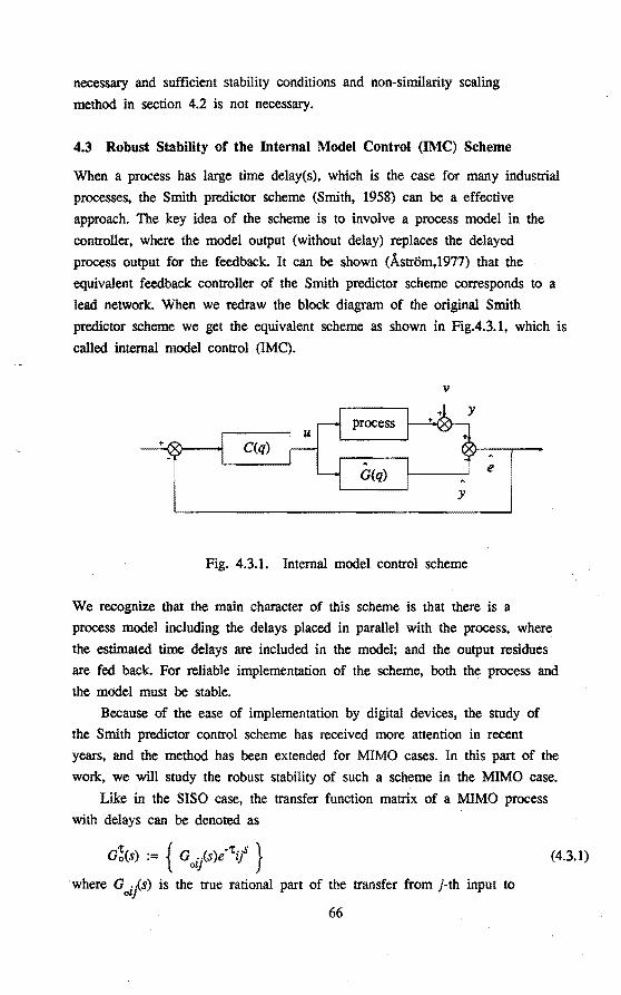
necessary and sufficient stability conditions and non-similarity sealing

metbod in section 4.2 is not necessary.

4.3 Robust Stability of the Intemal Model Control (IMC) Scheme

When a process has large time delay(s), which is tbe case for many industrial

processes, tbe Smitb predietor scheme (Smith, 1958) can be a effective

approach. The key idea of tbe scheme is to involve a process model in tbe

controller, where tbe model output (without delay) reptaces tbe delayed

process output for tbe feedback. It can be shown (Áström, 1977) tbat tbe

equivalent feedback controller of the Smith predietor scheme corresponds to a lead network. When we redraw the block diagram of the original Smitb

predietor scheme we get tbe equivalent scheme as shown in Fig.4.3.1, which is

called intemal model control (IMC).

ll

+

Fig. 4.3.1. Internat model control scheme

We recognize tbat the main character of tbis scheme is that there is a

process model including tbe delays placed in parallel with tbe process, where

the estimated time delays are included in tbe model; and tbe output residuès

are fed back. For reliable implementation of the scheme, botb tbe process and

tbe model must be stable.

Because of tbe ease of implementation by digital devices, tbe study of

tbe Smith predietor control scheme has received more attention in recent

years, and tbe metbod has been extended for MIMO cases. In this part of tbe

work, we will study the robust stability of such ·a scheme in tbe MIMO case.

Like in the SISO case, tbe transfer function matrix of a MIMO process

with delays can be denoted as

G!(s) := { G oip)e-'ti/ }

where G .1ls) is tbe true rational part of the transfer from j-tb input to

ol

66

(4.3.1)

i-th output, 't .. is the true time delay from u .(t) to y .(t). Similarly, the IJ J l

model transfer function matrix is denoted as

A

G't(s) := { êip)e-'ti/ }

where G .. (s) is the estimate of G .. (s) and 't .. is the estimate of 't ... IJ oiJ IJ lJ

Now the true process transfer function matrix is in the following class

= [G .. (s) + _ó .. (s) ]e-'ti/ IJ IJ

} \;f ij ' \;f (J)

Here the error is

.. ' ) G ( ) - ( 't .. -'t .. ) s G. ( ) u."s = .. se IJ IJ - .. s lJ ~ lJ

= G .. (s)e -.ó'ti/ - G .. (s) oiJ IJ

( 4.3.4)

which includes the errors in time delay estimates; and the upper matrix can

be determined by the same methods as in the previous chapter.

With these notations the block diagram in Fig.4.3.1 is equivalent as in

Fig.4.3.2 for studying the stability.

-o()()--~~ C(q) : u I

I

Fig. 4.3.2 Equivalent scheme of Fig. 4.3.1

(4.3.2)

(4.3.3)

Then, applying the Nyquist criteria to the system in Fig.4.3.2. and following

the same reasoning as for Lemma 4.2.2, we know that the system in Fig.4.3.1

is stabie if and only if

p[{ .ói/eiro)e-'tijro ) C(i~ ] < 1

Because

"iw ,"i.óeD

1\

s

:::::,. {I .óiJ(eiro)e-'tir =:; Mw)}

we have similar results as in the Theorems 4.2.1, 4.2.2 and 4.2.3 (with T 't "'t being replaced bt C): Assume that both Go(s) and G (s) are stable. Then we

67

(4.3.5)

(4.3.6)

can state:

(1) Singular value analysis. The system in Fig. 4.3.1 is stabie if

cr<A> cr<C> < 1 (4.3.7)

(2) Speetral radius method. The system in Fig. 4.3.1 is stabie if

p(AC) < 1 'r/ ro (4.3.8)

(3) Non-similarity sealing method. The system in Fig. 4.3.1 is stable, if

(4.3.9)

where L, R are defined similarly as in Theorem 4.2.3.

(4) Suboptimal salution of (3). The system in Fig. 4.3.1 is stable, if

[cr(L.M.> cr<R:1cL:1>1 < 1 'rfro (4.3.10)

where L • .R. are defined similarly as in (4.2.16).

Remark:- We see that in the intemal control scheme, the robust stability

tests become simpler; and the robust stability is related to the controller

•

and the upper bound matrix in a more transparent way, loosely speaking, the

stability criteria are proportional to the controller gains and the upper

bounds.

4.4 A Procedure from ldentification to Robust Control

After having tested the stability robustness of a feedback control system the

next logica! step is to analyze the robust performance of the system; cf.

Lunze (1989), Morari and Zafiriou (1989). But the result of this kind of

analysis will be very conservative. This is because that, when the upper

bound matrix A(ro) is used, it is very hard to derive some sensible

engineering measures of system performance without introducing considerable

conservativity for a MIMO system; cf. Lunze (1989). In our case a more

feasible approach is: (1) to check the nomina! system performance ,i.e.,

ignore the rnadelling errors, by a simulation; and (2) to check the robust

performance of the system by experimental tests. It is economically much

cheaper to perfarm this kind of experiment than the original identification

experiment: the system is under control, there are no extra excitations which

68

disturb the system and the experiment time can be shorter than that of the

identification experiment. This kind of tests must be feasible in case an

identification experiment is permitted.

The following procedure is proposed, see Fig.4.3.1, which will give the

reader a clear picture how the work in the previous chapters contributes to

linking identification and robust controL

Remarks on the procedure

Input design is an important issue in practice; and this problem will be

addressed in Chapter 6.

This procedure is not restricted to any specific control design

technique. Hence at the step of control design several controllers can be

designed with different techniques; the best one will be determined by the

following robust stability analysis and performance tests. This is not

difficult if some relevant CAD packages are available.

This procedure is iterative. When a controller can not pass the

stability or the performance test, the expression of the upper bound matrix

wiJl indicates directly or indirectly the ways for the redesign of the

identification experiment and/or the re-estimation of the models and/or the

redesign of the controller.

The work presenred in Chapter 6 follows this procedure.

69

•

Input design and identification

Nomina! model and upper bounds es tirnation

Control design r---------~~(PID,LQG,H ,IMC••)

"'

Robust stability analysis

No

?

Simulation and experiment tests of performance

Procedure 4.4.1 From identification input design to robust control

70

4.5 Conclusions

Robust stability analysis has been discussed in this chapter. Process model

uncertainty is described as structured perturbation. Three robust stability

analysis methods have been discussed and compared. The singular value

analysis method and speetral radius method are both simple, but the results

are conservative. The nonsimilarity sealing method makes best use of the

knowledge in the upper bound matrix which is best of the three methods with

respect to the conservarivity, but it needs some optimization procedure to

find the optimal sealing matrices. The suboptimal solution to the problem,

however, is easy to obtain, and gives better result than the speetral radius

method. The robust stability of internal model control scheme has been

studied as well; this scheme is specially useful when there are big time

delays, and those results are even simpler in the sense that the ralation

between robust stability and the controller become more explicit. The work

for searching the necessary and sufficiant robust stability condition is

still a chanlenge for the research.

All the results given here are computable; therefore they form part of

the basis for computer aided control system analysis and design.

Finally, a procedure for linking identification and robust control has

been proposed which shows that the work of Chapter 3 and this chapter can be

combined with many control system design techniques, such as PID, LQG, H00

,

and IMC to solve industrial control problems. At this stage the reader might

see how the theme of "integration" is being realized.

So far, the theories and techniques have been developed under the

assumption that the process is linear, time-invariant and stable. This can be

criticized easily because some nonlinearity and/or time-varlation is

inevitable in a real life industrial process, and the process can be nearly

unstable or even unstable. In the following chapter a scheme of combining

identification and control is proposed and stuclied which takes the above

mentioned difficulties into account and will extend the applicability of

linear systems and control theory and techniques.

71

Chapter Five

AN APPROACH TO LINKING IDENTIFICATION AND CONTROL

A scheme for identification and control is proposed in this chapter. This

method can overcome such difficulties as: the process in open loop is

unstable or nearly unstable, the noise level is too high, the process has

some nonlinearity and slight time-variation. In these cases open loop

identification with a linear and time-invariant model set may be very

difficult or inadequate. So the idea is: first apply a primary feedback

controller to the original process, for stabilization and diminishing of the

drawbacks mentioned; then identify this closed loop system using a linear

model set; fmally design a controller in the second loop in order to

optimize the overall system. It wiJl be shown that by this method one will

obtain a better model during the identification procedure, and that the two

loop system will not introduce restrictions for control under a condition

that is easy to check. For validating the idea, a case study is given. This

work extends the applicability of linèar system theory and techniques, such

as developed in previous chapters, to the solving of real life modelling and

control problems where the process is never completely linear and

time-invariant, and can be unstable.

5.1 Introduetion

The class · of processes considered here is assumed to be nearly linear and

nearly time-invariant. This implies that a linear time-invariant dynamic

model will give a reasonable approximation of the process behavior, so linear

control theory and design techniques are applicable to some extent. A typical

example of this class is an industrial process operating around a fixed

working point. The problem at hand is to control the process, in order to

improve or to optimize the performance of the whole system. The control

design is based on the estimated model. Now identification and controller

design are two aspects of the same problem, rather than two separate

problems. The "new scheme", discussed in this chapter means a new way of

integrating identification and control systern design procedures.

Often identification experiments have to be perfonned on systems

operating in closed loop. For industrial processes, in many cases, safety or

72

production-economie reasans do not permit open loop experiments, especially

when the process is unstable or nearly unstable. We will study the problem

mainly for such situations. In Section 5.2, the conventional approaches to

the problem will be briefly reviewed. In Section 5.3, the new solution to the

problem will be motivated; and in Section 5.4, the new scheme will be

analyzed and discussed. In order to validate this new method, a case study

will be given in Section 5.5. Conclusions and discusslons will be given in

Sectien 5.6.

Although the identification and control problem will be treated formally

by linear system theory, it is more realistic ro allow the assumption that

the true process has some nonlinearity and some time variation; and our

metbod is specially useful in practical situations when these effects have to

be recognized. Because there is no theory available to treat the problems of

nonlinearity and time-variatien in genera!, their effects will be discussed

intuitively based on the common knowledge, and also some laboratory

experiments will be used to support the method.

To explain the idea only single-input and single-output (SISO) processes

are used. But the theories and used bere hold for multi-input multi-output

(MIMO) processes too. This means that our metbod is suitable for MIMO

processes.

5.2 The Problem and Some Conventional Solutions

We shall start with the situation that an open loop identification experiment

is not allowed, due to the fact that the process is unstable or nearly

unstable, and/or the open process output would have too big a variance. We

will review briefly some of the conventional solutions to the problem, and

point out some of the difficulties when using these methods.

Manual Controt When the process dynamics are slow, an experienced operator

can control the process while rhe testing signa! is added at the process

input. The human operator can be seen as a feedback controller who stabilizes

the process and keeps the output varianee small. This is shown in Fig. 5.2.1.

The process input-output data are colleered for computing the process

dynamics.

Stabilization by human operator is unreliable or even impossible if the

process has fast dynarnics.

Identification of Processes in Closed Loop. This scheme is shown in Fig.

73

5.2.2, where P denotes the dynamics of the process, C denotes the controller.

The closed loop will be called "system". The signal u is called "process

input" and signal w is called "system input"; y is at the same time the

process and system output; and v is the process disturbance acting on the

process output.

tes ting sign~l-:.o<>--u-----1

V

y

Fig. 5.2.1 Experiment with manual control

V

w • u y

Fig. 5.2.2 Process identification in closed loop

In practice, the system input w is the testing signal (an extra

excitation) applied to the system in order to achieve a good identification

result. We will assume that w is persistently exciting and is also

measurable. Identification of processes when systems operate in closed loop

is called closed loop identification. This topic has attracted a lot of

interest and a great deal of literature has been dedicated to this problem.

This special area of identification has been studied and surveyed thoroughly

by Gustavsson, Ljung and Söderström (1977).

There are mainly three approaches to closed loop identification:

(1) The frrst method treats the process input-output data exactly as if they

were obtained from the open loop experiment. This method is called direct

identification.

(2) If the controller is linear and time-invariant, then an indirect way of

estimating the process parameters can be applied. The closed loop system can

74

be regarded as a whole and its parameters can be determined by some method.

In principle the open loop process parameters may then be determined from the

estimated closed loop system parameters using the knowledge of the

controller. This second approach is called indirect identification.

(3) The third method treats the process input and output jointly as the

output of a system driven by noise only. This is called joint input-output

identification.

The basic problems related to closed loop process identification are

process identifiabi/ity and accuracy aspects. The question of identifiability

is whether or not the process characteristics can be obtained as the number

of data tends to infinity; see Gustavsson et al., (1977) for the definition.

The problem of accuracy is related to the quality of the estimates for a

finite number of data.

Compared to an open loop experiment, the main problem caused by feedback

in the closed loop experiment for process identification is that the process

input u is correlated with the disturbance v. This correlation influences the

process identifiability and the accuracy of the estimation result. More

precisely, it makes things worse. For direct identification, correlation and

speetral analysis will not yield identifiability; the consistency of the

transfer function estimate is no Jonger guaranteed for output error method if

the output disturbance is not white noise. For joint input-output

identification, the same difficulties exist. For indirect identification, the

dynarnics of the closed loop system is operating in "open loop", the system

input w is independent of the disturbance v, see Fig. 2.2, therefore, no

restrietion regarding the estimation methods have to be introduced; for

example, correlation methods and the output error method will work well for

identifying the closed loop dynamics. In the second phase of indirect

identification the process dynamics is obtained from the closed loop system

dynamics and from the knowledge of the controller. This calculation can be

complex and it may or may not be successful.

Conceming identifiability and accuracy, the best way for closed loop

identification, shown by Gustavsson et al. (1977), is the direct

identification used with a prediction error estimation method, that assumes a

causa! relationship between the process input and output. "If they fail, no

other approach will succeed" (Ljung, 1987).

In genera!, prediction error identification methods need a iterative

minimization algorithm for computing the estimates, except in the case of

linearity in the parameters using an ARX (equation error) model. A necessary

75

condition for the success of the algorithm is that the predietors should be

stable. This condition is not guaranteed if the process is unstable or nearly

unstable, which is often the reason for closed loop experiments in practice.

Also some nonlinearity and/or time-varlation may cause the algorithm to fail.

So we see that even the best method for closed loop identification for the

process dynamics can easily fail in practice.

This is the moment to ask a question: For control system design, is it

really necessary to identify the process dynamics when the system is

operating in closed loop? The idea of the "new scheme" for solving

identification and control system design problem, is inspired by this

question.

5.3 The New Scheme

It is well known that feedback control can offer us the following benefits,

cf. Ashworth (1982) and Klein and Zaalberg van Zeist (1967):

decreasing the effect of nonlinearity;

decreasing the effect of time-variation;

attenuation of the effect of disturbances;

stahilizing the unstable process or improving the (relative)

stability; and

achieving desired dynamic characteristics.

All these properties of feedback control are concemed with the closed

loop system, not the original process. Consequently it is clear that feedback

will improve the result of closed loop system identification, if

identification techniques for linear processes are used. These nice

properties of feedback control are not helpfut for the original process

identification, as explained in the previous section.

Based on this observation, we propose the following solution to the

problem:

A Two Step Scherne to ldentification and Control for . Processes

The procedure:

1. Perform a closed loop experiment;

2. identification of the closed loop system dynamics, see Fig. 5.3.1

3. design the second loop controller for the closed loop system, based

on the closed loop system model, in order to improve or to optimize

the performance of the system, see Fig. 5.3.2.

76

w

Fig. 5.3.1

V

_J~ ~---

ldentification of the closed loop system

V

y

Fig. 5.3.2 Design of the second loop controller for the closed loop

Remarks

a. The first loop controller C1

is used to stabilize and/or to reduce the

output varianee and/or to reduce the effects of nonlinearity and the time

variation. In practice, C1

is determined based on some rough a priori

knowledge of the process dynamics, which is often available.

b. The identîfîcation part consists of only the first half of the indirect

identification method mentioned in the last section. Computation of the

process dynamics is skipped.

c. The closed loop system is operating in "open loop", so that the system

77

' input w is independent of the disturbance v. Therefore good statistkal

properties of identification of the closed loop system are guaranteed, the

estimation methods such as speetral analysis metbod and output error metbod

will work. Remember that they will usually fail for obtaining process models

in closed loop identification. It is clear that all the benefits of feedback

control are helpful for identifying the closed loop system dynamics.

d. The implementation of the second loop controller C2

is simple and

reliable: (1) if the two controllers are implemented in the same computer,

the new controller is C1

+ C2

• (2) If the first loop controller C1

already

exists, giving reliable operation, one does not need to remove it; the second

loop controller can be irnplemented in the computer. In case of computer

failure, set the output of the computer to zero; the system goes back to the

old control, no disaster will occur. This certainly will make the process

operator feel more comfortable to cooperate with you, because usually he will

not allow you to remove the existing controller with which he has a lot of

experience and feeling (both technica! and emotional).

5.4 Analysis of the New Scheme

In this section we will try to convince readers that: (1) the identified

system mqdel will have better quality than the process model; (2) in

practice, the two-loop structure in Fig. 5.3.2 will not introduce

restrictions for the overall control performance.

5.4.1 Some Notes on Approximate Modelling.

In applications an engineer usually thinks that feedback control "simplifies"

the dynamics, because most ·of (SISO) systems under feedback control will

behave like a low (second or first) order system, even the original process

is of higher order. However, when writing down the equations, a theorist

fmds that the closed loop system is always more complex than the original

process, because the order of the system dynamics is higher than ( or at least

equal to) that of the original process. Th is contradierion can be resolved by

making the distinction between approximate rnadelling and exact modelling,

which will be discussed in the following.

Since our knowledge about process dynamics (or in general about the real

world) is always limited and the data used for identification are noisy,

exact modeHing is never possible and not really necessary for many model

applications. This implies that identification is approximate modelling and

some model error is accepted. Notice that, in this work we use linear

78

time-invariant model sets for identifying the process (system) dynamics which

can have some nonlineacity and time-variation, this means that our starring

point is already approximate modelling. In this part, however, we will

discuss the problem of approximate modelling in the framework of linear

system theory, i.e., we assume that the process (system) is linear.

Denote G ciro) as the true transfer function of the process P. Suppose 0 ~

that the impulse response coefficients g(k) have been estimated somehow using

the data sequence

ZV= y(l),u(l), ...... , y(N),u(N) (5.4.1)

Denote the conesponding transfer function by GN(eiro) to emphasize that it is

an estimate based on N measurements.

The data sequence is assumed to be a realization of a random variabie

which, in turn, means that t~e es~imate GN(eiro) is a random variable.

If the expected value EGN(e1~ does not give a correct description of the

process, we say that the estimate is biased and denote the bias by

B(i~ := EGN(ei~ - G0(iro)

The varianee of GN(eiro) is

var[GN(eiro)] := EI GN(eiro) - EGN(iro) 12

Then, the mean square error of the estimate can be expressed by

This error can be used as a measure for the accuracy of the estimate.

(5.4.2)

(5.4.3)

(5.4.4)

There are two kinds of model errors: (1) structural error; and (2)

parametrical error. In the SISO case, if the model order is lower than the

order of the real dynamics to be identified, a structural error will occur.

In literature this situation is called that the process (system) is not in

the model set. Even if there is no structural error, i.e., the process

(system) is in the model set, the process disturbances and measurement noîse

will cause uncertainty in the model parameter estimates. In practical

situations, both structural and parameter errors occur, and the joint effect

of the two can be measured by the mean square error (MSE) of the estimates,

if the disturbances are modelled by stochastkal processes. The bias part of

MSE is caused by the structural (including the structure of the disturbance

model) error, while the varianee part of MSE is caused by the disturbances.

Most researchers admit parameter errors; a smaller number of researchers,

79

however, admit structural errors. We find that in the field of identification

and adaptive control, many authors assume that their processes (systems) are

in the model sets. The following example shows that the difference between

the exact order, with which one does not allow any structural· error, and the

approximate order, with which some structural error is allowed, can be very

large indeed. Norlee that for a SISO process, the model otder n defined in

Chapter 2 is equal to the McMillan degree of the process model, provided that

there are no common factors in the polynomials of the numerator and the

denominator in the model transfer operator G(q).

Example 5.4.1 Consider the first 1000 Markov parameters of a stabie frrst

otder process with a pole at a, I a I < 1 :

g(k) = i k = 1, 2, ···, 1000 (5.4.5)

Assume that there is only a small error e in the impulse response

measurements y(k) at k = 1000 so that

y(k) = g(k) k = l, 2, ... ' 999 (5.4.6)

y(lOOO) = g(1000) + e (5.4.7)

Then we have

The minimum order (McMillan. degree) of an approximate realization, which

interpolates the frrst 999 samples and ignores G(1000)+e, is 1. This is easy

to see.

The minimum otder (McMillan degree) of a pardal realization, which

interpolates all the 1000 measured samples, is 500 (see Damen et al. 1985). •

This is really a difference between heaven and heli!

We will allow that the model order is lower than the otder of the

dynamics to be identified; and the effect of feedback control on the

structural error will be discussed. In order to make some quantitative

discussion, we will frrst introduce some definitions.

Approximate Order and Exact Order. Consider a transfer function G(i~. the

otder n is defined as the degree of the denominator of its transfer operator

G(q). Let d'<i~ be A:th order approximation, k < n. Denote the additive

error as

!J.Gk(i~ = G(i~ - Gk(i00) (5.4.8)

Recent development of robust control theory shows that the infinity norm of

the transfer function and its error is a suitable measure for robust

80

controller system design. The infinity norm for a SISO stabie transfer

function G(ei00) is defined as

uG(ei~ll := sup I G()00) I

0<1 (5.4.9)

(jJ

Similarly for the error

nl\GA:.()~n := sup !liGk()00) I

0<> (jJ k' Then a proper measure for the error of G (e100

) can be

(5.4.10)

(5.4.11)

But this can not be evaluated because l\Gk(ei~ depends not only on G(i~. but also on the method of model approximation. In order to circumvent this

difficulty, some advance in model reduction will be introduced.

In recent years, the Ranke! matrix has played a very important role in

approximate modeHing (identification, model reduction)

design (H-infinity control). The Hankel matrix :H of a

G()00) is defined as the double infinite matrix

and control system

discrete-time process

[

g(l) g(2) g(3)···

:H := g(2) g(3) g(4)···

g(3) g(4) g(5)··· . . . . . .

where {g(k)}k=1,. .. ,oo is the impulse response of G(i00).

Denote n as the order of G(ei00), then it is well known that

rank(:H) = n

(5.4.12)

(5.4.13)

The n singular values of :H, h (G), ···, h (G), are called Hankel singular. 1 . n

values (HSV) of the process G(e1~; and, by convention, they are ordered

'ïli (5.4.14)

where h/G) is also called the Hankel norm of G()00).

Then we adopt from Glover (1984):

A Result on Model Reduction. Suppose that G(i~ is stabie and has order n.

Then it is possible to approximate G(i~ by a A:th order model Gk(i~. k < n, with the error bounded by

(5.4.15)

81

where ö S hk+2(G) +···+ hn(G) wiJl often be small. •

~is result shows that hk+l (G) is a suitable measure of the model error

AG"(e10) when a kth order model is used to approximate the nth order process

G(i«). The smaller h ... (G) is, the better the approximation will be. And, n.+l

also from Glover (1984), we know that

h1(G) < uG(i«)n.,.. (5.4.16)

Hence we have

(5.4.17)

Based on the above observations we give

Definition 5.4.1 The integer k is called A% error approximate order of the

nth order process G(i«), if

hk+l ( G) A = ( x 100 ) , and hkt

1 -:~; hkt

2 h1(G)

(5.4.18)

The minimum 0% error approximate order, which is n, is called exact order of

G(i«). •

In this definition the relative value of hkt1(G

0) is used to measure the

structural error of the kth order model approximation of the nth order

dynamics. As we see that by this definition, the approximate order is only

dependent on the distributions of HSV's of the process; hence it is a measure

of the character of the process dynamics. This definition can be used for

both continuoos-time and discrete-time processes, because the result of model

reduction holds for both cases; and it also holds for MlMO processes.

Remark-This definition is not suitable for the transfer function which has

large direct feed through (the D matrix of the state space realization). This

is because that the Hankel matrix can only reflect the dynamic properties of

the transfer function: the Hankel matrix will be zero if the order of

transfer function is zero. In the case that the direct feed through of the

transfer function is large compared to its Hankel singular value, the

following definition of the approximate order can be used instead of (5.4.18):

82

hk+ 1 (G) A=( xlOO),

max[ ID I, h1(G)]

and h :F h k+l k-t2

With this modification, the relation like (5.4.17) still holds and it will

become less conservative. In industrial applications, however, D = 0 for most

of the processes, hence definition (5.4.18) is suitable for our purpose.

Example 5.4.2 (Franklin et al., 1986) The transfer function (continuous

time) of a Boeing 747 model relating yaw rate (output) to rudder (input) and

the actuator at a working point is

0.475(s + 0.498)(s + 0.012 ± i0.488) GB(s) = (s + lO)(s +U.0073)(s + 0.563)(s + 0.033 ±z0.947)

The HSV's of G13(s) are

7.6265, 2.5707, 2.5569, 0.0209, 0.0179

and their relative values with respect to the first HSV, 7.6265, are

1, 0.3371, 0.3353, 0.0027, 0.0023

Then by Definition 5.4.1, we have

0 is the 100% error approximate order of G13(s);

1 is the 33.71% error approximate order of GB(s);

2 is the 33.53% error approximate order of G8(s);

3 is the 0.27% error approximate order of G8(s);

4 is the 0.23% error approximate order of GB(s);

5 is a 0% approximate order and, at the same time, the exact

order of G13(s); and

6 is a 0% approximate order, but not the exact order.

(5.4.19)

We see that a 3rd order model might approximate G3(s) very well. •

In view of approximate modelling, we could say that for a process, the

lower the approximate order is for a predefined error, the simpter the

dynarnics it has. The allowed error is determined by the intended use of the

model.

Based on the foregoing discussion, we have:

Conjecture 5.4.1 Feedback control can reduce the approximate order of a

process. That is, for the same A% error, the approximate order of the closed

loop system can be smaller than that of the original process; or,

equiva1ently, for the same approximate order, the A% error of the system can

83

be smaller than the .1% error of the process. •

Example 5.4.3 The control strategy for the Boeing 747 in Example 3.2 is

simply proportional feedback with a washout circuit (see Franklin et al., 1986). The feedback controller is then given by

C(s) = 1. 71s s + 0.33 (5.4.20)

The HSV's of the closed loop system are

7.5944, 0.2878, 0.2836, 0.0659, 0.0192, 0.0003

and their relative amplitudes with respect to the first HSV, 7.5944, are

1, 0.0379, 0.0373, 0.0087, 0.0025, 0.00004

We see that 1 is the 3.79% error approximate order of the system, which shows

that a frrst order model can give a reasonable approximation of the system

dynamics; remember that 1 is the 33.71% error approximate order of the

process. The exact order of the system is 6 which is higher than that of the

process. One also finds that for approximation orders 3 and 4, the

corresponding .1% errors of the system are greater than those of the process,

but the differences are small. •

Now the contradiction between the engineer and the theorist on the

complexity of process and system dynamics can be resolved: they are both

correct-the engineer thinks in view of approximate modelling, while the

theorist thinks in view of exact modelling.

5.4.2 Accuracy Aspects of the Process Model and System Model

Suppose that the closed loop experiment data is used with the predienon

w

I

I L

+

I

I I

----, I

V I I u I Y

[SYSteffil_ ~--

I I I I I

I .J

Fig. 5.4.1 Process identification and closed· loop system identification.

84

error metbod to identify both the process model and system model, as shown in

Fig. 5.4. 1. Assume that the number of data N is large enough to let us use

the asymptotic results in Theorem 2.3.1.

Denote the closed loop system model transfer function by

a;v<i~ (5.4.21)

and the real system dynamics by

G (=--"-)

+ G C o I

(5.4.22)

The mean square error of the estimates will be used as the measure of

accuracy.

Bias Term. It is well known that when the process (system) is in the model

set the bias of the estimate by the prediction error metbod tends to zero

when the number of data tends to infinity; see, e.g. Ljung (1987). In turn

this implies that if the identified dynamics are linear and time-invariant,

the bias part of the model error can be negleered when the model order is

high and the number of data is very large. For industrial processes N can be

very large when the experiments are performed in closed loop. In other words,

for this class of processes, the bias of the estimates are mainly caused by

the nonlinearity and/or the time variation of the identified dynamics. Hence,

if the process P has some nonlinearity and time variation, they will cause

bias if the linear time-invariant model is used to identify the process

dynamics. But if we consicter the closed loop system extended by the feedback,

it will have less nonlinearity and less time-variant dynamics than the

original process has. Therefore, the process nonlinearity and time varlation

will cause less trouble for the identification of closed loop system dynarnics

when the bias term is concerned. This part of the discussion is intuitive and

heuristic.

From the view of linear system theory, we have shown that the approximate

order of the closed loop system can be lower than that of the original

process. In such a case, this means that if the same approximate order is

used for the estimation of both the system dynarnics and the process dynarnics,

the bias of the system model will be smaller than the bias of the process

model.

Varianee Term. Heuristically, one could rewrite (2.3.78) as

85

(5.4.23)

where n is now also the McMillan degree of the model.

a) For dosed loop system identification

The input-output data sequence used. for system îdentificatîon is

i"= y(l),w(l), ...... , y(N),w(N) s

(5.4.24)

and the equivalent system output disturbance is

v (t) = S(q)v(t) •

(5.4.25)

where

S(q) = I (5.4.26) 1 + G

0(q)C

1(q)

is called sensitivity function. Then

~v(m) = ls(ifi)l 2~yCm) s

This shows that I S(ifi) I should be \<ept small for output varianee reduction;

smaller I S(ifi) I means better controL In practice I S(ifi) I has typically a

high pass character and is less than 1 over the low and middle frequency

range. Because the system input w and process disturbance v are independent, it

follows that

~ we(m) = ~ ew(m) = 0

Denote n as the approximate order of the closed loop system model, used s

in identification. From Theorem 2.3.1, we have

A • n ~ v ( 00 ) A. n <l> (m) Lo:>- • V I io:>-12 varf.Gi./.e Jl 9! N- ----• ...,.---= = N" -- S(e J (5.4.27)

<l>w(ro)R - <l>w/ro) <l>w(ro)

We see that better control (smaller IS I) will reduce

system model; this improves the

identification.

accuracy

b) For process identitication in closed loop

From the feedback relation

86

for

the varianee of the

closed loop system

u(t) = w(t) C1(q)y(t)

we have

u(t) = S(q)w(t) - S(q)C (q)H (q)e(t) I o

Denote n as the process model· order. Then from (5.4.23) we have p

From (5.4.28), we make the following observations:

(1) It is the system input w(t) (external excitation) that accounts for the

overall accuracy of the process transfer function estimate.

(2) Better control (smaller IS I) will lead to poorer accuracy of the process

model. This shows the well known conflict (dilemma) between process

identification and control in the closed loop.

c) Comparison

Because different objects are concerned in system identification and process

identification in closed loop, it is hard to compare (5.4.27) with (5.4.28).

After some calculation, a critica! reader will find that if we calculate

the closed loop system model from the process model, the calculated system

model will have the same varianee as given in (5.4.27), provided n = n and s p

when the first order approximation of the Taylor expansion is used for the

analysis. Then a question arises: what is the benefit of direct system

identification when the varianee of the estimate is concerned?

The answer to this question is twofold. First we argue that this analysis

has some error due to the approximation. Secondly we would like to remind

that a lower approximate order can be used for direct closed loop system

identification, in this case n < n and this means less varianee for closed s p

loop system identification.

5.4.3 The Optimality of the Two Loop System Structure

After the model of the closed loop system has been estimated the next step is

to design the second loop controller C2

based on the system model (and, may

be, also on the system noise model), see Fig. 5.3.2. Although it has been

shown that the identification with Jinear model sets can work better for

deriving the system model than for deriving the process model, one might

argue that the first loop controller C may introduce constraints for the I

second loop controller. The question is: does the system in Fig. 5.3.2 loose

87

the optimality, in other words, can the optima/ controller for the process he

realized by the two-loop structure? It will be shown here, under what

condition the two-loop system maintains optimality.

Let G (q) denote the transfer function operator of the process, and C (q) o I

denote that of the first loop controller C 1

• Then the transfer function

operator of the first loop system is

G (q) a•(q) = ___ o __ _

o 1 + G0(q)C

1(q)

(5.4.29)

In practice, the controller design chooses a controller from the class of

controllers which stabilize the process. If the process transfer function

operator and controller operator are both real rational, the set of all the

stahilizing controllers can be parametrized by Youla's lemma, see e.g.

Vidyasagar (1985).

Denote

!f(G (q)) := the set of all controllers which stabilize the 0

Similarly, denote

process G (q) 0.

!f(G8(q)) := the set of all controllers which stabilize the 0

closed loop system G'(q) 0

Then it is clear that the set of all controllers which stabilize the process

via the two-loop structure when c,(q) has been chosen is

!1/Go(q),C,(q)) := ( c,(q) + C/q) I C/q) E !f(G:(q)) }

We can now put the question in another way: Is it true that

(5.4.30)

(5.4.31)

(5.4.32)

Theorem 5.4.2 (Vidyasagar, 1985) Suppose G0(q) is real rational, C

1(q)

stahilizes G (q). Then 0

where properness of a rational function means that the degree of the

denominator is greater than or equal to the degree of the numerator. •

This result tells us that not all controllers in !f(G (q)) can be realized 0

by the two loop structure; the necessary and sufficient condition to make

88

such a decomposition possible is that C1(q) is proper and stabie a

condition which is easy to check and often satisfied in practice. A process

G (q) is said to be strongly stabilizable if J(G (q)) contains a stabie 0 0

controller. G (q) is strongly stabilizable if and only if the number of real 0

poles (counting the multiplicity) of G (q) between any pair of real zeros of 0

G (q) outside the unit circle is even (where one also has to count the zeros 0

at infinity ); cf. Vidyasagar ( 1985).

Summarizing, if the process G (q) is strongly stabilizable, by choosing 0

C/q) proper and stable, the optima! controller for the process can be

realized by the two-loop structure. Note that if C/q) is not proper and/or

not stable, this does not necessarily imply that the optimality of the two

loop system will be lost. If the optima! controller lies within the smaller

set !I/G0(q),C/q)), the optimality is still maintained; but the conditions

for this are not known yet.

During the design step the modelling error must be considered; then the

two-loop system structure in our case is expected to be superior to the

one-Joop structure. Concerning the robust stability, when designing the

second-loop controller, we are dealing with less restrictive gain and phase

margins compared to the design of the single loop controller, because we have

a better model for the closed loop system than for the process; this means

that we gain more freedom for improving the system performance.

5.5 A Case Study

Our case study concerns the identification and control of a bal! balancing

process which has been developed for research, education and demonstration

purposes (cf. Driessen, 1987); see Fig. 5.5.1. (All figures of this part are

gathered at the end of the section).

The metal ball rolls over a rail as a result of the change in the angle

of the rail. This change of angle is brought about by a servomotor. A voltage

is applied across resistance material on the rail from end to end and the

potential of the bal! is detected as a measure for its position. Using

controllers implemented on a PC, the ball is directed to a desired position

on the rail. The process input is the volrage supplied to the amplifier of

the servomotor, and the output is the ball position.

According to approximate physical modelling, the process has three poles

at the origin, and one real pole in the left half plane. The nonlinear part

of the servomotor is modelled as a dead zone, which is measured roughly and

compensated for by the PC. Then, the physical model of the process is given

89

by the following transfer function:

G(s) = 61 s3(s + 8.35)

(5.5.1)

S.S.l Results of ldentification

All experiments are performed at the sample frequency of lO Hz. The

experiment time is 100 seconds, hence the number of data N = 1000. The later

500 samples are used for identification, whereas the first 500 samples are

used for model validation.

The identification calculation is done by using the System ldentification

Tooibox of PC-Matlab.

Results from Manually Controlled Experiment Data. It is highly difficult to

control the ball balancing process by hand, due to its triple integration

behavior. After some training, manual control to keep the ball from the rail

ends is possible. As test signa!, white noise is used; so the process input

is white noise plus the manual control (swhich on and off) action, see Fig.

5.5.2.

After some experimentation, a 4th order model with one unit time delay is

chosen for the process. This is confirmed by the physical model (5.5.1). The

output error metbod gives the best result according to the validatien by

simulation; see Fig. 5.5.3. Predietien error methods fail to converge. From

Fig. 5.5.3 we see that the simulated output is quite different from the measured output. The reason for this bad fit can be:

(1) bad experimental condition (input satuation), see Fig. 5.5.2;

(2) instability of the process;

(3) nonlinearity of the process; and

(4) numerical problem in simulation.

We know that (2) and (3) cause numerical problems for estimation algorithms.

When a simulation model has poles very close to the unit circle, as in our

case, numerical problems can occur; see Áström and Wittenmark (1984).

Results of Process Identification from Closed Loop Data. The experiment .

scheme is shown in Fig. 5.3.1. The process input-output data is used for

process identification. Fig. 5.5.4 shows the process input and system input,

where the system input is the white noise test signa! with its varianee being

the same as the varianee of the test signa! in the manual control experiment.

90

The feedback controller is a discrete PDD controller and has the transfer

function:

2 c (q) = 46.2q - 85.8q + 40 I q2

(5.5.2)

Again, the predietien error method (ARMAX model) does not converge,

because the predietor is not stable; the output error method seems to

converges to a local minimum.

The process model has an order 4 with one delay. The output error model

is simulated, the simulated output is compared with measured output; see Fig.

5.5.5. We see that the result is not satisfactory. The reasous for this are

(2), (3) and (4) as discussed for the manual control data.

Because the output error method and general predietien error method do

not succeed for the process identification, the choise left for us is the ARX

model, which is equation error method. Hence a 4th order ARX model has been

estimated from the 1/0 data. This model is unstable, the poles of this ARX

model are:

1.0217 ± i0.0739, 0.8525, -0.7083

and the poles of the discrete physical model (with zero order holder) are:

1, 1, 1, 0.4339

This comparison tells us that quality of the ARX model is not very good. This

is, however, what we can achieve when we following the way. So this model

will be used for the single loop controller design which represent the

conventional method.

Results of Closed Loop System ldentification. The system input w and output

y are collected for the system identification, from the same closed loop

experiment as for process identification.

If the process has an order 4, and the controller is 2nd order, the exact

order of the system is 6. The results of identification show that order 3 is

high enough to model the system dynamics. For higher orders effective

zero/pole cancellation takes place. This is not surprising: for the

approximation of the system dynamics, order 3 appears sufficient.

The system model, therefore, has order 3 with one delay; remember that

the process model order is 4. The parameters are estimated by an output error

method. The simulated output is compared with the measured output in Fig.

5.5.6 and the fit is striking! This result should be compared with Fig.

5.5.5, where one wants to identify the process. The crosscorrelation function

91

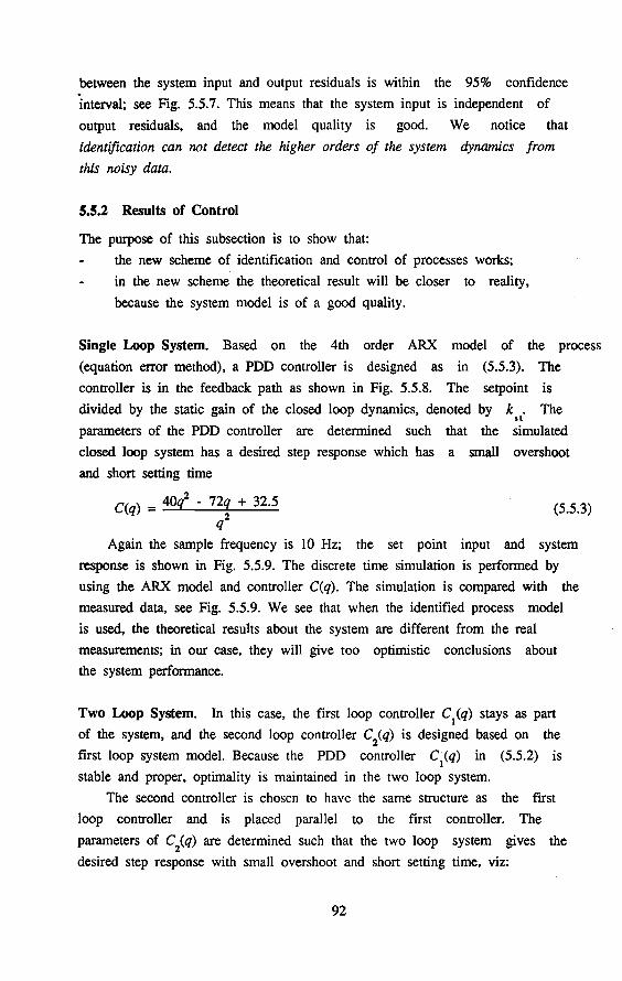
between the system input and output residuals is within the 95% confidence

interval; see Fig. 5.5.7. This means that the system input is independent of

output residuals, and the model quality is good. We notice that

identification can not detect the higher orders of the system dynamics from

this noisy data.

5.5.2 Results of Control

The purpose of this subsection is to show that:

the new scheme of identification and control of processes works;

in the new scheme the theoretica! result will be closer to reality,

because the system model is of a good quality.

Single Loop System. Based on the 4th order ARX model of the process

(equation error method), a PDD controller is designed as in (5.5.3). The

controller is in the feedback path as shown in Fig. 5.5.8. The setpoint is

divided by the static gain of the closed loop dynamics, denoted by k . The st

parameters of the PDD controller are determined such that the simulated

closed Joop system has a desired step response which has a smal! overshoot

and short setting time

2 C(q) = 40q - 72q + 32.5

l (5.5.3)

Again the sample frequency is I 0 Hz; the set point input and system

response is shown in Fig. 5.5.9. The discrete time simulation is performed by

using the ARX model and controller C(q). The simulation is compared with the

measured data, see Fig. 5.5.9. We see that when the identified process model

is used, the theoretica! results about the system are different from the real

measurements; in our case, they wiJl give too optimistic conclusions about

the system performance.

Two Loop System. In this case, the first loop controller C1(q) stays as part

of the system, and the second loop controller C2(q) is designed based on the

first loop system model. Because the PDD controller C1(q) in (5.5.2) is

stabie and proper, optimality is maintained in the two Joop system.

The second controller is chosen to have the same structure as the first

loop controller and is placed parallel to the first controller. The

parameters of C2(q) are determined such that the two loop system gives the

desired step response with small overshoot and short setting time, viz:

92

c2(q) = 6.0299l - 1~.86l6q + 5

q (5.5.4)

The digital feedback controller implemented in the PC for the process has

the form

C1(q) + C

2(q) = 52.2299l - 9~.6616q + 45

q

We see that controller implemented in the two loop

same order as the first loop controller, if C1(q) and

denominator.

(5.5.5)

structure will have the

C2(q) have the same

The two-loop system is shown in Fig. 5.5.10, where the set-point is

divided by the static gain of the two-loop system, denoted by k , which is st

measured from the step response.

The result of the experiment with the two loop system is compared with

the simulation result in Fig. 5.5.11, where the first loop system model and

second controller are used to simulate the two loop system. We find that the

simulation fits the real measurements very welL The measured output bas more

oversboot than the simulated output; this is probably caused by unmodelled

nonlinearities.

It is interesting to compare Fig. 5.5.9 and Fig. 5.5.11, where the single

loop simulation shows better step response than the two loop simulation, but

the real measurements show the opposite.

This case study shows that our proposal in Section 5.3 works well; and it confirms the discussions in previous sections.

93

Fig. 5.5.8

1 rail

2 metal balt

3 perspex tube

4 spindie

5 roll joining

6 end switches

7 servomotor

8 contra-weight

9 front side

10 turn axis (pivot)

11 flexible coupling

Fig. 5.5.1 Bali balancing process

Single loop system with PDD controller

Fig. 5.5.10 Two loop control system

94

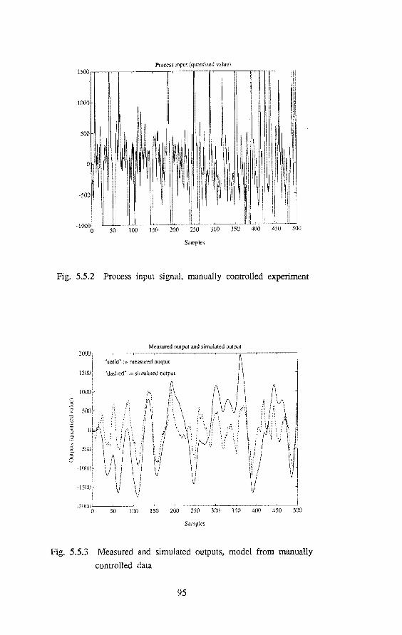
Processinput (quantized valuel

1000

500

0

-500

Samples

Fig. 5.5.2 Process input signa], manually controlled experiment

Measured output and sîmulated outpur

"solid" := measured output

200 250 300 350 400 450 500

Samples

Fig. 5.5.3 Measured and simulated outputs, model from manually

controlled data

95

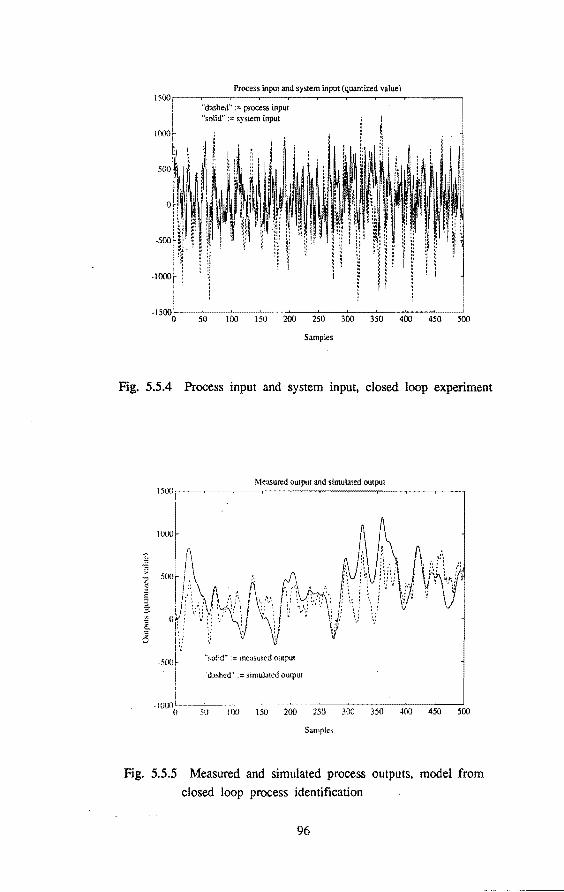
Processinput and system input (quantized value) 1500,----~-~--~-~-~---,---..--..---,.----,

"dashed'' := process input "solid" system input

1000

500

0

-I

0 50 100 150 200 250 300 350 400 450 500

Samples

Fig. 5.5.4 Process input and system input, closed loop experiment

-1000 1

{)

Measured output and simuiared output

"s.otid" :; measured output

'dashed" := simulated output

50 I()() 150 200 250 300 350 400 450

Samrles

500

Fig. 5.5.5 Measured and simulated process outputs, model from

closed loop process identification

96

-500

Measured outpur and simulated outpur

"sotid" := measured output

"da,hed" := simulated output

'Î . I~ 1\ l

NV \J\n 1 V Vj

350 400 450 500

Samples

Fig. 5.5.6 Measured and simulated process outputs, model from

closed loop system identification

lag

Fig. 5.5.7 Cross correlation function between the system input

and output residuals

97

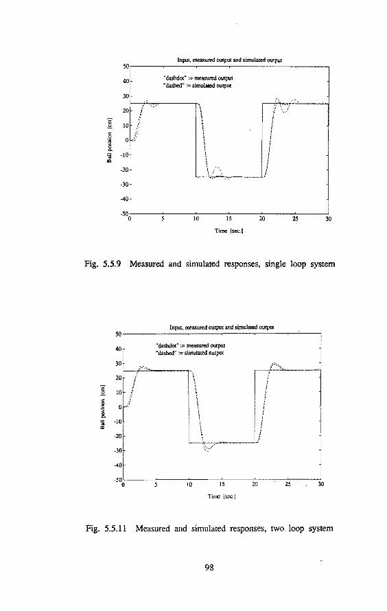
Input, measwed output and simuialed output 50,-----~------~----~------~------~-----,

40

30

20[' i :. 10 /.'

0 t

-20-

"dashdot" := measwed output "dashed" := simuialed output

\ \ \ ' l i l \ \ ' ..

/.:.. .,

l '. I

j I

i i I I

l ~~~~-------V

-50 '-------'-----'-----'---~---..___ __ _J

0 10 15 20 30

Time [sec.]

Fig. 5.5.9 Measured and simulated responses, single loop system

Ë 2. c

:~ s c. :;; IXl

50

40

30

20 I I

10 ! .~

0 li'

-10

-20r ·30r

:-·~~

Input, measwed output and simulated output

"dashdot" := measwed output "dashed" := simulated output

\ ! \ l \ : \ i ' ;

___ \~:--~------~·,/ - ·:\ ·-·.:~_.t"

-40L '50o --5~--~10----1~5 ---2~0 ______ 2,_5 __ ----,l30

Time [sec.]

Fig. 5.5.11 Measured and simulated responses, two loop system

98

5.6 Conclusions

In this chapter, a new way of integrating identification and control is

proposed. We have shown that it is possible to use the advantages of feedback

control to improve the quality of identification of system dynamics, while it

is well known that there is a conflict between feedback control and closed

loop identification of process dynamics, and the difficulties caused by

instability, nonlinearity and time-variation can not be overcome for process

identification in closed loop. Hence we propose: When the system operates in

closed loop for identification experiments, one can identify the closed loop

system dynamics; then design the second loop controller to meet the control

requirements; and the model of the original process is not needed in the

latter step. Any controller for the original process can be realized by the

two loop system structure, provided that the first loop controller is proper

and stabie which is true for many practical situations. The two loop system

is not new in control literature; see, for example, Vidyasagar (1985), where

the process model is assumed to be known and only the problem of control

design is addressed. But we believe that it is a new idea to combine

identification and control system design in such a scheme. The case study is

a successful example of the new method. Compared with conventional methods,

the advantages of our method are

solving the problem of identification/control for unstable processes;

reducing the difficulty caused by process nonlinearity, and

time-variation;

giving an implementation of the scheme which is both reliable and

simple.

These are specially beneficia! for identification/control of industrial

processes. The nice thing about this approach is that we do not have to pay

for the benefits gained, because the method neither needs to develop a new

identification theory/technique nor a control theory/technique; it is just a

new way of integrating identification and control; the key idea is to jump

out of the closed loop, and to view the system as a whole. The only condition

is that a sufficiently rich input is or can be applied to the closed loop

system.

The method can be used not only for situations where the closed loop

experiment has to be perforrned, but also for situations where the open loop

experiment is permitted. The advantages for the latter situation are the

reduction of the influences of nonlinearity, time-variation and disturbances

on the identification, and the increase in experiment time (due to the better

99

experiment condition).

This scheme can also be used to combine linear system theory and

techniques with nonlinear ones. For example, if the process P is severely

nonlinear, a nonlinear· controller C1

can be used for feedback linearization

(provided that P is linearizable); then normal linear identification

techniques can be used to obtain a linear model for the closed loop system;

and finally, based on this model, a linear second loop controller C 2

can be

designed to improve the system performance further.

100

Chapter Six

APPLICA Tl ON TO AN INDUSTRIAL PROCESS

6.1 Introduetion

In this chapter the theories and methods presented in Chapter 2 to Chapter 4

will be applied to an industrial process, the glass tube production process,

as introduced in Chapter 1.

ldentification and control for this process has been studied in Backx

(1987). Basically, his procedure consists of the following steps:

a Select the input and the output variables

As discussed in Chapter 1, the decision was: input 1 is mandril pressure;

input 2 is drawing speed; output 1 is wall thickness; and output 2 is

diameter.

b Determine the input signals for the identification experiment

Two PRBNS (pseudo random binary noise sequence) signals were used as the

input testing signals. The clock frequency of the PRBN signals is the same as

the sampling frequency; this means that the inputs are white-noise-like

testing signals with respect to the process dynamics.

c Pre-processing of the measured input/output data

This step includes peak-shaving, detrending, offset correction, time delay

estimation and correction.

d Process model estimation

First a FIR (finite impulse response) model with order 50 has been estimated

(by output error least squares) from the pre-processed 1/0 data. Then a model

reduction has been applied to the FlR model to obtain a minimal polynomial

start sequence of Markov parameters (MPSSM) model (see Back, 1987, for the

definition); the parameters of such a model have been estimated by using the

1/0 data again with an output error method. Fînally the irrelevant modes of

the MPSSM model have been removed by a model reductîon and a model with a

state space realization has been obtained.

101

e Control system design

The internal model control scheme was used, because there are large time

delays at the process outputs. The other advantages of this scheme are:

It allows for independent control of the process dynamics and

disturbance reduction.

The analysis of robust stability is simpter than the analysis for normal

feedback scheme, and the relation between the robust stability and the

controller dynamics is more explicit; see Chapter 4.

The block diagram A of the control system is shown in Fig. 6.1.1. P denotes the

process dynamics; G is the process model; F is the state feedback from the

model, applied both to the model and to the process. Note that observer

technique can not be used here due to the large time delays. F was designed

such that the process model with the state feedback will have desired

dynamical behavior such as good step response and nearly decoupled transfer

matrix. K 1 is a constant matrix, which equals the inverse of the steady cl

state transfer matrix of the process model with the state feedback. sf is a

filter matrix which was designed for disturbance reduction.

The developed control strategy has been implemented on the glass tube

process and it brought an enorrnous improvement on the quality of the

production; see Fig. 6.1.2.

After some period of successful production, the process engineer asked:

"Is improvement possible for funher disturbance reduction?" The work

presented here is to answer this question. We will follow Procedure 4.4.1,

proposed in Chapter 4; the work of Back can be seen as the first iteration of

this procedure. In Section 6.2 the existing control system is examined and

analyzed. In Section 6.3 a new identification experiment is perforrned and a

new model is estimated and validated. In Section 6.4 the feedback filter Sr

is adjusted for flirther disturbance reduction. In Section 6.5 we will draw

the conclusions.

6.2 Exarnining and Analyzing the Existing Control Systern

In the internat model control scheme of Fig. 6.1.1, there areA at least two

places where improvements are possible: the process model G and the feedback

102

filter matrix sf Because tbe input signals and tbe identification metbod are tbe most

important factors wbicb determine tbe model quality, there is a need to

exarnine if these two are tbe most appropriate cboices; and tbis examinatien

sbould be based on tbe intended use of tbe model. As mentioned in tbe

previous section, the process model G bas been estimated from tbe I/0 data

wbere tbe inputs are wbite-noise-like PRBNS signals; and tbe identification

metbod is basically an output error metbod. Wben taking a closer look at the

control system in Fig. 6.1.1, we find tbat tbere are at least two

applications of tbe process model, tbe first one is on-line simulation and

the second one is to design tbe feedback filter matrix S( A model wbicb is

most suitable for tbe simulation purpose need not be (usually can not be) the

best for tbe feedback controller design. So, ideally speaking, we need

different models of the same process for different purposes. Of course, to

keep the work simple we will try to use tbe same model for different

applications, provided tbat these applications need models with similar

properties.

For tbe use of simulation, it is know tbat the output error metbod is the

most appropriate one. Wbat about tbe input signals? First of all, tbe actual

process inputs (wbicb will be the simulation inputs for tbe model) are never

wbite noises in a closed loop control system. Fig. 6.2.1 compares the the

spectra of the measured process inputs during the feedback control and of the

frequency responses of the modeL We see tbat the power of the these

simuiatien inputs is concentraled at very low frequencies, wbich are not at

all white noises. Our pbysical feeling or engineering intuition suggests that

for the estimation of a simulation model, the testing inputs must resembie

tbe cbaracters of the actual simuiatien inputs; in our case, this means that

it is necessary to put more power at tbe low frequencies for the testing

input signals. The quantitative study of this problem will be done in the

next section.

The use of tbe feedback filter matrix Sr is for disturbance reduction and

maintaining the closed Joop stability; and these two demands are often

conflicting factors. In case of internal model control schemethe feedforward

design technique can be used to design tbe filter matrix.

This can be explained as follows: Assume tbat tbe process model is

perfect, i.e., the model error is zero, then the control system in Fig. 6.1.1

becomes an open loop contiguration and tbe output residuals are equal to the

output disturbances; cf. Fig. 6.2.2. Denote S (J~ as tbe transfer function me

103

matrix of the process with the state feedback; if

there will be total disturbance cancellation at the system outputs. This,

however, is not applicable due to the following limitations:

St must be causal, i.e., the filters should be proper.

sf should be stable.

(6.2.1)

Due to time delays, there is a limit frequency above which the

disturbance rednetion is no ·tonger effective. Denote ro as the limit 0

frequency and 'td as the largest time delay, then

Ol0

S! 1t/td (radls) (6.2.2)

The gain of the filters are restticled by the consideration of robust

stability (modelling errors are taken înto account bere).

Under these limitations, only some approximation of (6.2.1) is possible. A

practical design is to choose the filter matrix sf which follows:

Filter Design Rules 6.2.1:

1) sf consists of proper and stabie filters;

2) sf approximates the frequency responses of the ideal filter sfid of

(6.2.1) in the frequency interval [0, ro); sf tends to zero in the frequency

interval [ro , 1t]; and 0

3) in the frequency interval [0, roo), the gains of the filters of sf are

limited by the robust stability contraint •

The frequency responses of the ideal filter matrix is a diagonal dominant

transfer function matrix. This is because the state feedback achieves a

nearly decoupled transfer. The existing filter matrix is also diagonal,

consisting of two identical first order lowpass filters. Fig. 6.2.3 compares

the used low order filter and the ideal filter. We find that the difference

between the two is quite large. This conservative choice of the filter was

due to the fact that, at that time, there was no knowledge about the · model

uncertainty in the frequency domain available, and in order to guarantee the

robust stability, the gains of the filters had to be kept small.

When the upper bound matrix of the modeHing errors becomes available,

then we can test the robust stability of the existing system. This test will

teil if one can atain more disturbance reduction, which implies the increase

104

of the filter gains. Fig. 6.2.4 shows the results of the test, where three

methods are used: singular value analysis method, speetral radius method and

the suboptimal solution of the non-similarity sealing method; and the 2cr

bound is used for the varianee part of the modelling errors. For this system,

the non-similarity sealing method gives the best result; and the speetral

radius method is sometimes better than the singular value analysis method at

some frequencies, worse at other frequencies. We find that the system is

robustly stabie and that there is still some room . for increasing of the gains

of the feedback filter matrix.

In summary, the analysis and examinatien of the existing system indicate

that, in order to reduce the simulation error of the process model and to

achieve more disturbance reduction, there is a need to improve the model

quality at low frequencies; this can be done by proper design of the

identification input signals. And there is a possibility to increase the

feedback filter gain without the loss of stability robustness.

6.3 Input Design and Model Validation

From the discussions of the previous section, we know that for the simulation

purpose it is necessary to increase the model quality at low frequencies. We

will chose the input signals such that the estimated model is best for the

use of simulation, and the same model will be used for the feedback filter

design. In order to keep the discussion simple, the SISO case will be

treated; there is no principle diference in the MIMO case.

Optimal input spectrum for high order FIR models

When estimating high order FIR models the bias of the model is negligible,

hence only the influence of the varianee is considered.

Now let us assume that the model is used for simulation. Denote u'(t) as

the simulation input with spectrum <l>~(ro) (which is in general different from

the spectrum of the input used in the identification experiment). Then the

simulated output is:

;(t) = GJ:fq)u5(t) (6.3.1)

where GJ:fq) is the n-th order FIR model; and the simulation error is:

e(t) [G~(q) - G0(q)]u'(t) (6.3.2)

This error has the varianee

105

1t A • '

V = S I G~(e1~ - G (e1ro) l 2èP~(ro)dro e -1t o

One can choose the input spectrum such that

1t A o

EVe = S var[G~e1~]·èP~(ro)dro -1t

is minimized. Applying Corollary 2.3.2 it follows that

n 1t èPv(ro) EVe 9! N S ~ -«l>~(ro)dro

-1t u

(6.3.3)

(6.3.4)

(6.3.5)

It can be shown (see Yuan and Ljung, 1985) that the optimal input should have

the spectrum

(6.3.6)

where 11 is a constant which is adjusted with respect to the input amplitude

constraint. This result is physically very appealing: it says that the

process should be excited more at those frequencies where the simuiadon

input has more power and where disturbances make more trouble. Notice that

this spectrum is not related to the process transfer function. In practice,

u'(t) is (partly) known and v(t) can be measured from the process output when

keeping the input constant. Hence the estimated «l>~(ro) and 4>/ro) are

available. This means that the optima! input spectrum can be determined

before identifying the process transfer function.

It can be shown (see Lenssen, 1988) that for MIMO processes, under the

assumption that the testing input signals are mutually independent, the

optimal input spectrum for the i-th input is given by

«l>~~(ro) = 11/«l>~.(ro)-.! èP v .<ro) l I J =I J

(6.3.7)

The optimal input spectrum for the estimation of the FIR model of the

glass tube process has been calculated, based on the input signals measured

from the closed loop system and the output disturbances measured · from the

open loop experiment when keeping the inputs constants; see Fig. 6.3.1. What

we see is that the power of the optima! inputs concentrate at very low

frequencies; this confrrms our physical feeling.

106

Optimal input spectrum for low order models

In the case of low order model estimation, the process dynamics is not in the

model set, therefore, both the bias contribution and the varianee

contribution to the simulation errors should be minimized by choosing the

proper input spectrum.

(1) Minimfzing the varianee contribution

The asymptotic expression of the varianee in Chapter 2 gives a reasonable

approximation for low order models, see Ljung (1985). Hence, following the

same reasoning for deriving (6.3.6), we know that it also gives the optima!

input spectrum which minimizes the varianee contribution for the low order

model.

(2) Minimfzing the bias contribution

Based on the work of Yuan and Ljung (1985), as it can be shown that the

optima! input spectrum which minimizes the bias contribution, for FIR models,

is

This result is also physically appealing, it says that the optima! input

spectrum should be proportional to the simulation input spectrum.

(6.3.8)

We have only presented .the results which treat the bias contribution and

varianee contribution separately for low order models. A more general study

of the problem can be found in Yuan and Ljung (1985).

The Choice for the Glass Tube Process

It is clear that for the estimation of the high order FIR model, the input

spectrum given by (6.3.7) is optimal. For the low order estimation, the

optima! input spectrum for minimizing the bias contribution will in general

be different from that for minimizing the varianee contribution. For the

glass tube process, however, our observation is that these two spectra are

nearly the same; compare Fig. 6.2.1 with Fig. 6.3.1. This implies that the

optima! input for the high order FIR model estimation is also (nearly)

optima! for the low order model estimation for the glass tube process.

Therefore, the input spectrum given in (6.3.7) will be realized for the new

identification experiment; and the measured 1/0 data will be used for both

the high order FIR model estimation and low order model estimation.

107

Each of the realized time domain signals which approximate the desired

spectrum, consists of two PRBNS signals, one with a clock period much larger

than that of the "white noise" PRBNS signal, and the other is a "white noise"

PRBNS with a small amplitude; see Fig. 6.3.2. Let us eaU this a colored

PRBNS signa!.

In order to check if the new model really has a higher precision at low

frequencies, the static gains (DC gains) of the old and new models are

compared with the measured DC gains in Table 6.3.1. We see that the DC gains

of the new model are indeed much closer to the measured ones.

Table 6.3.1 Checking the DC gains of the old and new models

Errors of t he white PRBNS model

Errors of t he colored PRBNS model

DCII

21 .6%

8.3

DCI 2

9.4%

DC21 DC2 2

28.6% 67.7%

9.0% 2.2%

Another way of validaring the models is to supply the simulation inputs

(u5(t)} to the process and to the two models; and then compare the simulation

errors of the two models. This experiment has not been performed.

6.4 Readjustment of the Feedback Filter

As we have seen, the existing feedback filter was more for robust stability

than for disturbance reduction. The robust stability analysis for the old

filter and the new model is shown in Fig. 6.4.1, which again tells that we

can do more for disturbance reduction without distabilizing the system. Now

the problem is how to tune the filter matrix S( The process model has zeros

outside the unit circle (non-minimum phase), and has large time delays. This

means that the ideal filter given in (6.2.1) is unstable and improper, which

makes the filter design difficult. The Nyquist plots of the ideal filters are

shown in Fig. 6.4.2. Following the Filter Design Rules 6.2.1, the used filter

needs to have positive phase at low frequencies in order to have good

disturbance reduction; and the filter gain should decay very fast at higher

frequencies. This, however, is very difficult to realize when the complexity

of the filter matrix is restricted, which is the current situation.

When taking a good look at the Nyquist plots, we find that the identity

matrix, i.e., no filter, will approximate the ideal filter better than the

108

old filter at very low frequencies; see also Fig. 6.4.3. Although the

"identity filter" does not follow the Filter Design Rules 6.2.1, i.e., its

gains do not decay at higher frequencies, we expect some better disturbance

reduction at very low frequencies. Fig. 6.4.4 compares the disturbance

reduction of the old filter and the "identity filter" in the ideal case,

i.e., when assuming the model to be perfect as in Fig. 6.2.2, where measured

disturbances are used for the simulation. The result of the simulation shows

that about 25% reduction of standard deviation at both outputs can be

achieved with the identity filter.

Before we use the identity filter, the robust stability of the system

should be checked. Fig. 6.4.5 shows that the robust stability test criterion,

the sub-optimal solution of the non-similarity sealing method, is greater

than 1 around frequency 0.5 (rad/s) and also at very high frequencies. We

should take this as a warning that the system with the identity filter can be

unstable. Now we have two choices: (1) to go back to perform re-modelling

and/or redesign; and (2) to ignore the warning and imptement the identity

filter.

Let us see what we can do if we take the first choice. Following the

Procedure 4.4.1, we can perform another input design and identification

experiment, this can influence the varianee part of the modelling errors, cf.

Chapter 3, but it is expensive. We can also perform another model reduction,

e.g. take a higher order model than the used one; this can reduce the bias

part of the modelling eqors. Fig. 6.4.6 shows the upper bound matrix , bias

part and 2cr bound of the varianee part respectively. We find that the bias

part of the modelling errors is greater than the varianee part around the

frequency of 0.5 (rad/s) and at highest frequencies; this implies that a

better model reduction will be more effective than a new input design for

improving the model quality in order to achieve more stability robustness.

Another thing we can do, following Procedure 4.4.1, is to reduce the filter

gain from the frequency 0.5 (rad/s) where there is no need for disturbance

reduction, see Fig. 6.4.8, which can easily be done.

Actually, the second choice is not unreasonable. We know that the robust

stability analysis is conservative due to:

The upper bounds are not very tight, because the varanee of the

estimates is proportional to the model order, and this implies that estimated

low order model (with order 6) has much smaller varianee than the high order

FIR model (with order 50), but this is not reflected in the calculation of

the upper bounds (the asymptotic normality does not hold for low order

109

models); and also because an inequality is involved in deriving the upper

bounds; cf. Chapter 3.

The sub-optima! solution of the non-similarity sealing metbod is only a

sufficient stability condition for the whole class of the processes described

by the low order model and the upper bound matrix.

Being aware of the conservativity of the robust stability analysis, and also

noticing that the sufficient stability condition is violated only in a smal!

band of frequencies, we are quite sure that the system with the idenrity

filter is stable.

Fig. 6.4.7 compares the control result of the old filter with the old

model and that of the "identity filter", i.e., no filter, with the new model.

The system is stabie indeed! The new control achieves more disturbance

reduction at very low frequencies, and less at higher frequencies, which was

expected. Fig. 6.4.8 shows the results in the frequency domain, which makes a

clearer demonstranon of the results.

Discussions about the experimental tests

The test results agree with the theoretica! predicrions about the model

quality, stability and the disturbance reducrion. The better disturbance

reducrion at the very low frequencies is the joint effect of a better model

quality and a better approximation of the ideal filter at those frequencies.

The differences between the simulation test of the two filters (Fig. 6.4.4)

and the real test (Fig. 6.4.7) are mainly due to the modelling errors, and

the differences of the process dynamics and disturbances: the simulation

study used the model and the measured disturbances from the process when it

was operaring at another woricing point.

Large time delays (about 15 samples in this case) cause no difficulties

for disturbance reducrion in this system. This is because the disturbances

are very slow signals. Fig. 6.4.8 shows that the bandwidth of the

disturbances is about 0.1 (rad/s), this is lower than the limit frequency

imposed by the time delays which is about 0.2 (rad/s).

There is a need to increase the order of the low order model, in order

to reduce the bias part of the modelling errors; cf. Fig. 6.4.6.

Much better disturbance reducrion can be achieved if more complex

feedback filters can be used to approximate the ideal filters in the

frequency interval [0, 0.1] (rad/s). This better approximarion implies that

the filter gains will be slightly greater than 1 at those frequencies, cf.,

110

Fig. 6.2.3, but it will not cause a stability problem, because there is still

some freedom left in the frequency interval [0, 0.1] (rad/s) for higher

filter gains; cf. Fig. 6.4.5.

6.5 Conclusions

In this chapter we have tested the theory and the methods developed in

Chapter 2 to Chapter 4. The results are convincing. The input design is

another use of the asymptotic theory, which makes it possible to do practical

experiment design with respect to the intended use of the model. The model

validation conflrmed that the new model has a better quality than the old

model at low frequencies. The availability of the upper bound matrix of the

modeHing errors have made it possible to analyze the robust stability of the

existing system; and the result of this analysis has indicated conservativity

of the existing system which brought the hope for further improverneut of the

control performance. Due to the current limit of filter complexity, the

improverneut of disturbance reduction is not so significant. But this is not

the end of the story, the important achievement of this experimental test and

the analysis is that we see the possibility of obtaining much better

disturbance reduction and we know how to do it, which was not clear before

this study.

A good theory should work. After the experience of the real test, we are

more confident about the applicability of our theory and methods. We have

reached what we wanted: to build a bridge which links identification and

control system design; and to let identification serve for industrial process

controL

111

setpoint

soaled watl thickness

o.

scated diameter

o. samples

Fig. 6.1.1 The control scheme

''I I t

10.000 0.

10.000 o.

scaled wal! thickness

scaled diameter

Fig. 6.1.2 Result of the existing control

112

V

y

10.000

samples 10.000

() c._::,__~-~c:---0 (l.l 0.2 0.3 0.4 0.5 0.6 0.7 0.8

Frequency (rad./sec.)

0.1 0.2 0.3 0.4 0.5 0.6 0.7 0.8


Transfer funcrion 1 2

0.8

0.2

0.6L 0.4. . ..... J~ 0.2

0 0 1 2 3 4

Transfer function 2 2

oL-~~======~--~ 0 2 4

Frequency (rad./sec.) Frequency (rad./sec.)

Fig. 6.2.1 Comparison of the band width of the simulation inputs

and the model danymies

113

V

y

Fig. 6.2.2 Equivalent scheme of Fig. 6.1.1 when the model is perfect

Compare the ideal filters and the old filters

___ old filter (1, 1) and (2,2)

02 0.3 0.4 0.5 0.6 0.7 O.X

Frequency (rad./sec.}

Fig. 6.2.3 Comparison of the frequency responses of the filters

114

0.8

Robust stability tesiS for old filter and old model

"solid":=non-similarity sealing mehtod (sub-optim;ll

"dasbed":=specual radius mehtod

"dotted":=singular value analysis mehtod

0.3 0.4 0.5 0.6 0.7 0.8


Fig. 6.2.4. Robust stability tests of the existing system

0.1 0.2 0.3 0.4 0.5 0.6 0.7 0.8

Frequency (rad)sec.}

20~~·· SP<ftrum of optima! inp?t 2

1 15

10~

:L ~~ 0 01 ()2 0.3 0.4 0.5 0.6 0.7 0,8

Frequency (rad./sec.}

Fig. 6.3.1 Spectra of the optimal input signals

115

4~~~~~~~~~~~~~~~~~~~ o ~ g a ~ ~ ~~ 1a ~~ ~ ~

Samples

a a ~ 10 ~~ 1a ~~ ~ ~

Samples

Fig. 6.3.2 Colared PRBNS as the identification input signals

Robust stability test for the old filter and new model

1.4

1.2

stability bound

1 --------········ ............ ----------------------------.---.----- .. -.-----

0.8

0.6

0.4

1.5 2 2.5 3 3.5

Frequency (radJsec.)

Fig. 6.4.1 Robust stability of the old filter and the new model,

suboptimal of the non-similarity sealing mathad

116

0 < ~

2

0

-1

-2

-3 -4 -3 -2 -1 0 2

REAL

Fig. 6.4.2 The Nyquist plots of the ideal and old filters

ro E [0, 0.3] (rad./sec.)

''dashed":=old filter, pole at 0.95

"solld":=identity fitter •.

0.1 0.2 0.3 0.4 0.5 0.6 0.1 0.8

Differenees between !he ideal filter and used filters 22 20

15 ~

10

"solid":=identity filter

0.1 0.2 0.3 0.4 0.5 0.6 0.1 0.8

Frequency (radJsec.)

Fig. 6.4.3 Differences between the ideal and the other filters

117

0 500 1000 1500 2000 0 500 1000 1500 2000

500 1000 1500 2000 500 1000 1500 2000 Samples Samples

Fig. 6.4.4 Disturbance reduction of the two filters,

simulation, setpoint is zero

Robust stabilitytest for the identity filter and new model 2.-----~----~----~----~----~----~-.---,

1.8

1.6

!.4

stability bound

o'~-~~-~- ~-~---~------'"--~------' 0 0.5 1.5 2 2.5 3.5


Fig. 6.4.5 Robust stability test of the system with identity filter,

suboptimal of the non-similarity sealing mathod

118

0 I 2 3 4


O.ZS ~--i"U'ill!!nne:L'T ~bou~nd:!.:l li2.1l,t,2'i-\--,

0.6,.--

0.4

0.2

2


Fig. 6.4.6 Upper bounds (solid), bias part(dotted), and

2a bound of the varianee part (dashed)

I LOl~

O!d ,control, ',"•!! thickt'ess new control wall thickness

0.99

0 500 1000 1500 2000 0 500 I 000 1500 2000

0.995 '---~---~-·-~-----l 0 500 1000 1500 2000

samples samples

Fig. 6.4.7 Comparison of the old and the new control

119

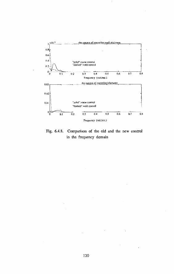
"solid":=new control "dashed":"old control

0.2 0.3 0.4 0.5


0.6

003~ the s ctra of controlled diameter

002:

() OI \ "sohd".=new control l\ "dashed" .=old control

0~ • 0 0.1 0.2 0.3 0.4 0.5 0.6


0.7 0.8

0.7 0.8

Fig. 6.4.8. Comparison of the old and the new control

in the frequency domain

120

Chapter Seven

CONCLUSIONS

The problem of identification and control of MIMO industrial processes has

been studied in this work. The effort has been put on the inlegration of

these two branches in the field of systems and controL We believe that only

by good combination of the two, one can fully make use of the actvances of the

available theories and techniques.

In Chapter 2 the asymptotic theory of black-box transfer function

estimates has been developed; based on the theory, in Chapter 3, the upper

bounds of the errors in transfer function estimates has been defined and the

algorithms for estimating both the nomina! model of the process and the upper

bound matrix of the model uncertainty, have been proposed. The stochatical

approach is taken for modelling the uncertainties in the signals and the

models, which is conventional in process identification. All the results

developed are computable and numerically simple. By the combination of high

order model estimation and model reduction one can avoid the difficult task

of MIMO model structure selection; and the asymptotic theory can be applied

naturally to this procedure to derive the upper bound matrix of the modelling

errors. Notice that the asymptotic theory can also be used for input design,

as described in Chapter 6.

In Chapter 4, we have summarized some results of robust stability

analysis, and shown how the upper bound matrix, which is a "structured"

description of model uncertainty, can be used readily for testing the

stability robustness of MIMO linear feedback systems.

In Chapter 5, we have argued that, for control design, process

identification in closed loop--a problem which has been studied extensively

in the literature-is not rea!ly necessary. Instead, we have proposed to

identify the closed loop system dynamics, and then design the second loop

controller based on the closed loop system model. In this scheme,

identification and control become mutually supporting; and the two loop

system will maintain optimality under realistic conditions. The case study

fully supports the idea.

Chapter 6 validates the work in a real industrial application. The input

design has shown another use of the asymptotic theory. The estimated upper

121

bound matrix of the process modelling errors has been used for analyzing the

stability robusmess of the existing controlled system, and the result has

indicated that there was still some freedom for improving the control of the

glass tube production process. The previously discussed control strategies

have been tested on the real proèess and the results are convincing. Now we

can tell that the theories and the methods developed in this work are indeed

applicable for industrial applications.

Further research is needed to tighten the upper bounds, if possible. To

search for the necessary and sufficient condition for the robust stability is

an interesting topic. And also more effort is needed to study the

approximation of an unstable and noncausal transfer function by a stabie and

causal one, which is important for the feedback controller design in the

internat model control scheme; see Chapter 6.

Basically, in this work, we have done two things: the ftrst is the

derivation of the upper bound matrix which bridges the gap between

identification and robust control (Chapter 2, 3, and 4); the second is the

proposal of a scheme for identification and control, which combine the two in

a natural way (Chapter 5). Both ideas follow, and are inspired by, the

philosophy of integration; they are tested by real life experiments, one in

laboratory, one in factory. This shows that indeed some philosophical

thoughts can be beneficia! for research and development. We believe that more

work can be done in systems and control along the line of integration.

122

KEFERENCES

Ashworth, M.J. (1982). Feedback Design of Systems with Significant Uncertainty. Engineering dynamics and control monograph series, John Wiley & Sons Ltd., UK.

Áström, K.J. (1977). Frequency dornain properties of Otto Smith regulators. Int. J. Control, Vol. 26, pp. 307-314.

Áström, K.J. ( 1980). Maximum lîkelihood and predietien error methods. Automatica, Vol. 16, pp. 551-574.

Áström, KJ. and P. Eykhoff (1971). System identification - a survey. Automatica, Vol. 7, pp. 123-162.

Áström, K.J. and B. Wittenmark (1984). Computer Controlled Systems: Theory and Design. Prentice-Hall, Englewood Cliffs, NJ ..

Áström, K.J. and B. Wittenmark (1989). Adaptive Contro/. Addison-Wesley, Reading.

Backx, T. (1987). ldentification of an lndustrial Process: A Markov Parameter Approach. Dr. Thesis, Dept. EE., Eindhoven University of Technology, Eindhoven, The Netherlands.

Backx, A.C.P.M. and A.A.H. Damen (1989). Identification of industrial MIMO processes for fixed controllers-part 1 and part 2. Journal A, Vol. 30, pp. 3-12, and pp. 33-43.

Berman, A. and R.J. P1emmons (1979). Nonnegative Matrices in the Mathematica/ Sciences. Academie Press, New York.

Beuningen, E. van (1988). ldentification for Robust Control. Master thesis, group Measurement and Control, Dept. EE., Eindhoven University of Techno1ogy, Eindhoven, The Netherlands.

Boekhoudt, P. (1988). The H00

Control Design Method: A Polynomial Approach.

Dr. Thesis, University of Twente, The Netherlands.

Brillinger, D.R. (1975). Time Series: Data Analysis and Theory. Holt, Rinehart and Winston, New York.

Capra, F.(1984). The Tao of Physics. Bantam Books, Toronto.

Capra, F.(1983). The Turning Point. Bantam Books, Toronto.

Cloud, DJ. and B. Kouvaritakis (1986). Statistica! bounds on multivariable frequency response: an extension of the generalized Nyquist criterion. lEE Proc., Vol. 133, Pt.D., pp. 97-110.

Damen, A.A.H., R.P. Guidorzi, A.K. Hajdasinski and P.MJ. Van den Hof (1985). On multivariable partial realization. Int. J. Control, Vol. 41, pp. 589-613.

123

Damen, A.A.H., Y. Tomita and P.M.J. Van den Hof (1985). Equation error versus output error methods in system identification. Intemal report ER/06, Group Measurement and Control, Dept. EE., Eindhoven University of Technology, Eindhoven, The Netherlands.

den Brinker, A.C. (1989). Modelling the Transient Visual System. Dr. Thesis, Eindhoven University of Technology, Eindhoven, The Netherlands.

Doyle, J.C. (1982). Analysis of feedback systems with structured uncertainty. JEE Proceedings, Part D, Vol. 129, pp. 242-250.

Doyle, J.C. and G. Stein (1981). Multivariable feedback design: concepts for a classicallmodem synthesis. IEEE Trans. Autom. Control, Vol. AC-26, pp. 44-16.

Driessen, M.H. (1987). Realization of a Mechanica/ Test Process for Education Purposes (in Dutch). Master thesis, Group Measurement and Control, Dept. EE., Eindhoven University of Technology, Eindhoven, the Nether lands.

Eykhoff, P. (1974). System ldentiflcation: Parameter and State Estimation. John Wiley & Sons, New York.

Francis, B.A. (1987). A Course in H00

Control Theory. Lecture Notes in Control

and lnformation Sciences, Vol. 88, Springer-Verlag, Berlin.

Franldin G.F., J.D. Powell and A. Emami-Naeini (1986). Feedback Control of Dynamic Systems. Addison-Wesley, Massachusetts.

Gevers, M and L. Ljung (1986). Optimal experiment design with respect to the intended model application. Automatica, Vol. 22, pp. 543-554.

Glover, K. (1984). All optimal Hankel-norm approximations of linear multivariable systems and their L

00-error bounds. Int. J. Control, Vol.

39, pp. 1115-1193.

Grimble, M.J. (1986). Optimal H00

robustness and relationship to LQG design

problems. Int. J. Control, Vol. 43, pp. 351-372.

Gunnarsson, S. (1988). Frequency Domain Aspects of Modeling and Control in Adaptive Systems. Dr. Dissertation, Dept. EE., Linköping University, Linköping, Sweden.

Gustavsson, I., L. Ljung and T. Söderström (1977). Identification of processes in closed loop Identifiability and accuracy aspects. Automatica, Vol. 13, pp. 59-75.

Hann, E.J. and C.C. Heyde (1972). On limit theorems for quadratic functions of discrete time series. Ann. Math. Stat., Vol. 43, pp. 2258-2066.

Heij, C. (1988). Deterministic Jdentification of Dynamica/ Systems. Dr. Thesis, University of Groningen, Groningen, The Netherlands.

Janssen, P.H.M (1988). On Model Parametrization and Model Structure Selection for Jdentification of MIMO Systems. Dr. Thesis, Eindhoven

124

University of Technology, Eindhoven, The Netherlands.

Jenkins, G.M. and Watts (1968). Speetral Analysis and lts Applications. Holden-Day, San Francisco.

Kailath T. (1980). Linear Systems. Prentice-Hall, Englewood Cliffs, N.J ..

Klein, G. and J.J. Zaalberg van Zeist (1967) Precision Electronics, Cleaver-Hume Press Ltd. London.

Kosut, R.L. (1986). Adaptive calibration: an approach to uncertainty modelling and on-line robust control design. Proc. 25th Conf Decision and Contra/, Athens, Greece, December, 1986, pp. 455-461.

Kouvaritakis, B. and H. Latchman (l985a). Singular-value and eigenvalue techniques in the analysis of systems with structured perturbations. Int. J. Contra/. Vol. 41, pp. 1381-1412.

Kouvaritakis, B. and H. Latchman (1985b ). Necessary and sufficient stability criterion for systems with structured uncertainties: the major principal direction alignment principle. Int. J. Control. Vol. 42, pp. 575-598.

Kwakernaak, H. (1985). Minimax frequency domain performance and robustness optimization of linear feedback systems. IEEE Trans. Autom. Control, Vol. AC-30, pp. 994-1004.

Kwakemaak, H. (1986). A polynomial approach to minimax frequency domain optimization of multivariable feedback systems. Int. J. Control, Vol. 44, pp.117-156.

Lenssen, M. (1988). Optima/ Input Design for MIMO Processes. Master Thesis, Dept. EE., Eindhoven University of Technology, Eindhoven, The Netherlands.

Ljung, L. and P.E. Caines (1979). Asymptotic normality of prediction error estimation for approximate system models. Stochastics, Vol. 3, pp. 29-46.

Ljung, L. (1985). Asymptotic varianee expressions for identified black-box transfer function models. IEEE Trans. Autom. Control, Vol. AC-30, pp. 834-844.

Ljung, L. and Z.D. Yuan (1985). Asymptotic properties of black-box identification of transfer functions. IEEE Trans. Autom. Control, VoL AC-30, pp.514-530.

Ljung, L. (1987). System Identification: Theory for the User. Prentice- Hall, Englewood Cliffs, N.J..

Lunze, J. (1984). Robustness tests for feedback control systems using multidimensional uncertainty bounds. Syst. & Cont. Letters, Vol. 4, pp. 85-89.

Lunze, J. (1989). Robust Multivariable Feedback Control. Prentice Hall, New York.

Miller, K.S. (1974). Complex Stochastic Processes: An Introduetion to Theory and Application. Addison-Weslley, Inc., London.

125

Morari, M. and E. Zafrriou (1989). Robust Process Control. Prentice-Hall, Engtewood Cliffs, N.J..

Needham, J. (1962). Science and Civilization in China. Vol. 1, Cambridge University Press, Cambridge.

Ogata, K. (1980). Modern Control Engineering. Prentice-Hall, Engtewood Cliffs, N.J..

Owens, D.H. and A. Chotai (1984). On eigenvalues, eigenveetors and singular values in robust stability analysis, Int. J. Control, Vol. 40, pp. 285-296.

Smith, O.J.M. (1958). Feedback Control Systems. McGraw-Hill Book Company, Inc., New York.

Söderström, T. and P. Stoica (1989). System ldentification. Prentice-Hall, New York.

Sternad, M (1987). Optima/ and Adaptive Feedforeward Regulators. Dr. Thesis, Uppsala University, Uppsala, Sweden.

Van Broekhoven, E. (1987). On a bound of black-box modelling errors. Report of Practical Project. Dept. EE., Eindhoven University of Techno1ogy, Eindhoven, The Netherlands.

Van den Hof, P.M.J. (1989). On Residual-Based Parametrization and ldentification of Multivariable Systems. Dr. Thesis, Eindhoven University of Technology, Eindhoven, The Netherlands.

Vidyasagar, M. (1985). Control System Synthesis: A Factorization Approach. MIT Press, Cambridge, Massachusetts.

Wahlberg, B. (1985). Connections between system identification and model reduction. Technica/ Report LiTH-/SY-1-0146, Dept. EE., Linköping University, Linköping, Sweden.

Wong, K.C. and L-T. Wu (1936). History of Chinese Medicine. AMS Press, New York.

Yuan, Z.D. and L. Ljung (1984). Black-box identification of multivariable transfer functions: asymptotic properties and optimal input design. Int. J. Control, Vol. 40, pp. 233-256.

Zames, G. (1981). Feedback and optimal sensitivity: model reference transformations, multiplicative seminorms, and approximate inverses. IEEE Trans. Autom. Contra/, Vol. AC-26, pp. 301-320.

Zames, G. and B.A. Francis (1983). Feedback, minimax sensitivity, and optimal robustness. IEEE Trans. Autom. Control, Vol. AC-28, pp. 585-601.

Zhu, Y.C. (1987). On the bounds of the modelling errors of black-box MIMO transfer function estimates. BUT-Report 87-E-183, Dept. EE., Eindhoven University of Technology, Eindhoven, The Netherlands.

Zhu, Y.C. (1988). On the bounds of the modelling errors of black-box MIMO

126

transfer function estimates. Proc. 8th IFACIIFORS Symp. on Identification and System Parameter Estimation, Beijing, P.R. China, pp. 734-739.

Zhu, Y.C. (1989a). Estimation of transfer functions: asymptotic theory and a bound of model uncertainty. Int. J. Control, Vol. 49, pp 2241-2258.

Zhu, Y.C. (1989b). Black-box identification of MIMO transfer functions: asymptotic properties of predierion error models. Int. J. Adaptive Control and Signa/ Processing, VoL 3, pp. 357-373.

Zhu, Y.C., M.H. Driessen, A.A.H. Damen and P. Eykhoff (1988). A new scheme for identification and controL EUT-Report 88-E-2I3, Dept. EE., Eindhoven University of Technology, Eindhoven, The Netherlands.

Zukav, G. (1979). The Dancing WU U Masters: An Overview of the New Physics. Fontana, London.

127

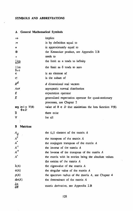
SYMBOLS AND ABBREVIATIONS

A General Mathematica! Symbols

:=

À.im lim ~0 E

c

Rd

AsN

E

E

arg min V(9) 8eD

3 'r;f

B Matrices

À.(A)

cr(A)

p(A)

det(A)

à A ëJH

implies

is by definition equal to

is approximately equal to

the Kronecker product, see Appendix 2.8

tends to

the limit as n tends to infinity

the limit as ö tends to zero

is an element of

is the subset of

d dimensional real veetors

asymptotic normal distribution

expectation operator

generalized expectation operator for quasi-stationary

processes, see Chapter 2

value of 9 e D that minimizes the loss function V(9)

there exist

for all

the (iJ) element of the matrix A

the transpose of the matrix A

the conjugate transpose of the matrix A

the inverse of the matrix A

the inverse of the transpose of the matrix A

the matrix with its entries being the absolute values

the entries of the matrix A

the eigenvalue of the matrix A

the singular value of the matrix A

the spectrum radius of the matrix A, see Chapter 4

the determinant of the matrix A

matrix derivative, see Appendix 2.B

128

I, lp

colA

identity matrix, identity matrix with dimeosion pxp

column operator stacking the columns of the matrix A

on top of each other, see Appendix 2.B

C Signals, processes and models

u(t)

y(t)

v(t)

{ e(t)}

z!l Rit)

~('C) u< ro) p

{go(k)}k=l ··· oo ' '

{g(k)} k=l ... 00

' ' {ho(k)}k=l ··· oo

' ' {h(k)} k=J,. .. ,oo

e, e, e ·l q

0

G (q) 0 ~

G(q), G(q)

G(i~ 0

C(q), C(ei~

ó(i00)

b.(ro)

uG(i~u 00

m-dimensional input vector at time t

p-dimensional output vector at time t

p-dimensional output disturbance vector at time t

p-dimensional white noise vector

input/output data sequence, see Chapter 2

autocorrelation function matrix of u(t)

estimated Ru(t), see Chapter 2

auto specxtrum matrix of u(t)

process dynamics

impulse response of the process

impulse response of the process model

impulse response of the disturbance filter

impulse response of the disturbance model

parameter vector, its estimate and the true value

delay operator

the transfer operator of the process

the model and the model estimate of the process

transfer operator

the transfer function (frecquency response) matrix of

the process

the model and the model estimate of the process

transfer function matrix

the transfer operator and the transfer function matrix

of the feedback controller

modelling errors of the transfer function estimates

upper bound matrix of the modeHing errors

infinity norm of the transfer function matrix, see

Chapter 5

129

D Abbreviations

w.p.

ARMA

ARMAX

ARX FIR

IMC

I/0 MA

MIMO SISO

sv

with probability, see Chapter 2

Auto Regressive Moving Average

Auto Regressive Moving Average eXogeneous

Auto Regressive eXogeneous

Finite Irnpulse Response

Intemal Model Control

Input/Output

Moving Average

Multi Input Multi Output

Single Input Single Output

Singular Value

130

Curriculum Vitae

ZHU Yu-Cai was bom in Bole, Xinjiang Province, China, on 17 April, 1960.

From October 1978 to July 1982 he studied at Department of Information and

Control, Xi'an Jiaotong University, China; where he obtained bachelors degree

of engineering. From July 1982 to August 1983 he was a teaching assistant at

Xi'an Jiaotong University. From August 1983 to October 1985 he studied at

Department of Electrical Engineering, Eindhoven University of Technology, The

Netherlands; and he obtained Ir. (M.Sc) title. From January 1986 to February

1990 he was a research assîstant at Department of Electrical Engineering,

Eindhoven University of Technology. He is now with Process Identification

Unit, Datex Industry, 's-Hertogenbosch, The Netherlands.

131

CORRECTIONS

1) On page 2, the last line should read: "Just as it does not make sense

to ask which is more important for life, the sun or water, it does not

make sense to say yin or yang is good or bad. What"

2) In Chapter 4, on page 61, Lemma 4.2.2 and the proof should be:

Lemma 4.2.2 The system in Fig. 4.2.1 is stabie if and only if

p[öC(l+GC)'1J < 1 'ïloo

proof "If part"-Suppose that

det[l + EilC(l+GC)'1] 0 for some oo, ö and E

then -1 is an eigenvalue of EÖC(I+GC)'1• But

p[EilC(/ + GC)'1] :::; p[öC(l + GC)'1]

and hence

p[öC(/ + êC)-11 :::: 1

This contradiets (4.2.7).

"Only if part"-First we will show that

'ïiEE[O, 1)

p[roC(/ + GC)-1] * 1 'ï!Ee[O, 1), 'ïlöeD,

is a necessary condition for (4.2.6). If for some !lED, and some E so that

p[roC(I + êcr1J = 1

then 3 ae "R such that, for the same ö and E

À.[E(eiaö)C(/ + GC)-1] -1

but ciaA)eD, hence (4.2.6) is violated. ' Now suppose that 3 such that

p[öC(/ + GC)'1] > 1

then 3 Ee [0, 1], such that, for the same !lED

p[EilC(l + GC)'1]

and (4.2.6) is violated.

'

(4.2.7)

•

D

STELLINGEN (PROPOSITIONS)

behorende bij het proefschrift

"ldentification and Control of MIMO Industrial Processes:

An Integration Approach"

van

ZIIU, Yu-Cai

Eindhoven, 13 februari 1990

I

A system is a complex entity fom1ed of many interrelating elements subject to

a common plant or serving a common purposeY1 There are two basic properties

of systems: dynamic property and organic property. If a system is dynamic it

means that its behavior involves or includes time-dependent operations. If a

system is organic it means that it is life-like, its elements have the

ability of processing information (reasoning) and making decisions. Another

important feature of an organic system is its inseparability: its elements or

subsystems will behave in a totally different way or will cease to exist,

when they are separated from the system. System theory can describe the

dynamic property to some extent, but the Jack of recognition of the organic

property in system theory hampers its applicability to the study of

biological, social and economical systems, which are all organic systems.

c11 Sage, A.P. (1987). In Systems & Control Encyclopedia. Pergamon Press,

Oxford, Vol. 7, p. 4767.

II

In systems and control literature, very little attention has been paid to

feedforward compensation (in the case of measurable disturbances): in the

book by Astrom and Wittenmark (1984), in total only one page is devoted to

this topic; in the 8 volume Systems & Control Encyclopedia (Pergamon Press,

1987) only two terms are related to this topic. This shows some imbalance in

the field of systems & control.

III

Uncertainty is the enemy of accuracy in modelling, prediction and control.

But a modelling approach which tolerates uncertainty will describe the

(uncertain) reality more accurately than an approach which does not recognize

uncertainty. Quantum mechanics and Kalman filter are the proof.

IV

One of the main goals of adaptive control is to compensate for time

variations of the process behavior. But in theoretical analyses of adaptive

control systems, a common assumption is that the process is not time variant.

This implies that paradox is allowed in academic research. In fact, this is

the rule rather then the exception.

v The main cause of conflict in world politics and in social life is not the

conflict of interests to be found in the different parties, but the

misunderstanding and mistrust between them.

VI

In early times, the computer was a simple system. There was only one CPU

(central processing unit) which controlled every thing in the system. Later

the computer system became more complex, and more CPU's were added; but one

of them had the highest priority and controlled other CPU's and the whole

system. At present the computer system has become even more complex and the

trend is decentralization, i.e., no CPU should have the absolute power.

This reminds us of the evolution of society.

Due to

spectral

the causal relations

analysis it is more

VII

between

natural to

the

use

process inputs

asymmetrical

and outputs,

windows than

in

the

normally used symmetrical windows, for the estimation of the process transfer

functions; see Chapter 3 of this thesis.

VIII

Assume that the process is linear and

noise filter is stable. Then it can

identifiable under the prediction error

identification literature.

IX

In Chapter 6 of this thesis we find

time invariant, but unstable,

be shown that the process

method. This fact ., is hidden

and the

is not

in the

that the "identity filter", which does

not filter, can do a better job than the ex1stmg low pass filter for

disturbance reduction; cf., Fig. 6.4.4 and Fig. 6.4.7. This tells us that

sometimes nothing is better than something.

x

A conference or symposium is meant for communication, but some people come in

order to show that they can make something, which others do not understand.

II

identification and control of mimo industrial processes : an integration approach · identification...

Documents