identification of dangerous contingencies for large scale...
TRANSCRIPT

1
Identification of dangerous contingencies for large scale power system security assessment
Florence Fonteneau-Belmudes
Department of Electrical Engineering and Computer ScienceUniversity of Liège, Belgium
PhD defense - March 1st

2
1. Introduction
Electric power systems - structure

3
1. Introduction
Power system security assessment - objective
➢ what Transmission System Operators (TSOs) want to avoid:
+ →
contingency degradation of the security of the system
normal situation

4
1. Introduction
Power system security assessment – notion of contingency
➢ definition:
any unexpected event triggering a change in the current operating conditions;
➢ examples:
- equipment outages (the simultaneous loss of k equipments is called an N-k contingency);- transient faults;- error of an operator;
➢ note:
the notion of contingency can also be used to model the uncertainties on the future generation and load patterns.

5
1. Introduction
Power system security assessment - usual practice
➢ using models of their network and simulation tools, TSOs simulate the occurrence of each potential contingency;
➢ the contingencies leading to unacceptable operating conditions are classified as dangerous;
➢ for each dangerous contingency, adapted preventive or corrective control actions are designed to preserve the level of security of the system.

6
1. Introduction
Large scale power system security assessment
➢ the size of the set of potential contingencies grows with the size of the studied system and with the considered time horizon;
➢ when the contingency space is too big, it is no longer possible to analyze each contingency individually in a reasonable amount of time;
➢ traditional solutions:
- increase of the computational resources and parallelization of the security assessment task;
- use of filtering techniques to determine thanks to some light computations which contingencies to simulate.

7
1. Introduction
Large scale power system security assessment
➢ problem considered in this thesis:
- we address large scale power system security assessment problems with bounded computational resources (not allowing an exhaustive screening of the contingency space);
- we consider that only detailed contingency analyses are performed;
➢ proposed approach:
we propose an algorithm exploiting at best the number of contingency analyses that can be carried out so as to identify a maximal number of dangerous contingencies.

8
1. Introduction
Definitions
➢contingency severity:
based on the definition of an objective function O : X → ℝ (where
X is the contingency space) that quantifies the effect of each contingency on the operating conditions of the system;
➢ dangerous contingencies:
contingencies x such that O(x) ≥ Í, where the threshold Í is defined by the user;
➢ computational resources:
a fixed budget in terms of CPU time, expressed as a maximal number of evaluations of the objective function that can be performed.

9
1. Introduction
Reformulation of the problem addressed in the thesis
➢problem statement:
identify a maximal number of contingencies x such that O(x) ≥ Í while evaluating the function O a bounded number of times.
➢ procedure developed to solve it:
an iterative sampling framework inspired from derivative-free optimization algorithms.

10
Outline
1. Introduction
2. An iterative sampling approach based on derivative-free optimization methods
3. Embedding the contingency space in a Euclidean space
4. Case studies
5. On-line selection of iterative sampling algorithms
6. Estimating the probability and cardinality of the set of dangerous contingencies
7. Conclusion

11
Comparison with an optimization problem
➢usual formulation of an optimization problem:
given a search space X and a real-valued function f : X → ℝ,
identify an element x0 in X such that f (x
0) ≥ f (x) 8 x 2 X ;
➢ problem addressed here:
given a search space X, a real-valued function O : X → ℝ and
a real number Í, identify a maximal number of points w in X such that O(w) ≥ Í with a bounded number of evaluations of the function O.
2. An iterative sampling approach based on derivative-free optimization methods

12
Comparison with an optimization problem
➢ the configuration (search space and objective function) is the same;
➢ we do not only want to identify one maximum of the objective function, but the set of points such that O(x) ≥ Í ;
➢ if Í = max O(x), our problem is equivalent to a classical
optimization problem aiming at identifying all the maxima of the
objective function.
2. An iterative sampling approach based on derivative-free optimization methods
x 2 X

13
Specificities of our ''optimization-like'' problem
➢the search space is very large;
➢we want to be able to solve this problem in a generic way, whatever the contingency space and objective function at hand;
➢no derivative of the objective function is available, and only the pairs (x,O(x)) can be used for solving the problem;
➢ since the objective function can only be evaluated a given number of times, the number of such pairs (x,O(x)) is bounded.
2. An iterative sampling approach based on derivative-free optimization methods

14
Derivative-free optimization algorithms
➢ they only use values taken by the objective function for different points of the search space to search for a maximum of this function;
➢they are split into different categories:
- algorithms building models of the objective function based on samples of its values;
- algorithms directly exploiting sets of values of the objective function and iteratively trying to improve a candidate solution to the problem.
2. An iterative sampling approach based on derivative-free optimization methods

15
Our basic iterative sampling (BIS) algorithm for dangerous contingency identification: illustration
➢considered problem:
2. An iterative sampling approach based on derivative-free optimization methods
O (x)
x
Í9

16
Our basic iterative sampling (BIS) algorithm for dangerous contingency identification: illustration
➢ first iteration: drawing a sample of points from ℝ according to an initial sampling distribution;
2. An iterative sampling approach based on derivative-free optimization methods

17
Our basic iterative sampling (BIS) algorithm for dangerous contingency identification: illustration
➢ first iteration: evaluating the objective function for all the points of this sample;
2. An iterative sampling approach based on derivative-free optimization methods

18
Our basic iterative sampling (BIS) algorithm for dangerous contingency identification: illustration
➢ first iteration: selecting the ''best points'' of the current sample to compute a new sampling distribution;
2. An iterative sampling approach based on derivative-free optimization methods

19
Our basic iterative sampling (BIS) algorithm for dangerous contingency identification: illustration
➢ second iteration: generating a new sample according to this updated sampling distribution;
2. An iterative sampling approach based on derivative-free optimization methods

20
Our basic iterative sampling (BIS) algorithm for dangerous contingency identification: illustration
➢ second iteration: generating a new sample according to this updated sampling distribution;
2. An iterative sampling approach based on derivative-free optimization methods

21
Our basic iterative sampling (BIS) algorithm for dangerous contingency identification: illustration
➢ third iteration: the points in the current sample are located in a tighter area around the maximum of the objective function;
2. An iterative sampling approach based on derivative-free optimization methods

22
Our basic iterative sampling (BIS) algorithm for dangerous contingency identification: illustration
➢ third iteration: the points in the current sample are located in a tighter area around the maximum of the objective function;
2. An iterative sampling approach based on derivative-free optimization methods

23
Our basic iterative sampling (BIS) algorithm for dangerous contingency identification: illustration
➢ fourth and last iteration: the current sampling distribution is now focused on the maximum of the objective function;
2. An iterative sampling approach based on derivative-free optimization methods

24
Our basic iterative sampling (BIS) algorithm for dangerous contingency identification: illustration
➢ fourth and last iteration: the current sampling distribution is now focused on the maximum of the objective function;
2. An iterative sampling approach based on derivative-free optimization methods

25
Our basic iterative sampling (BIS) algorithm for dangerous contingency identification: illustration
➢ a large majority of the points drawn from the contingency space during the execution of the algorithm are dangerous contingencies;
2. An iterative sampling approach based on derivative-free optimization methods
Í9
26
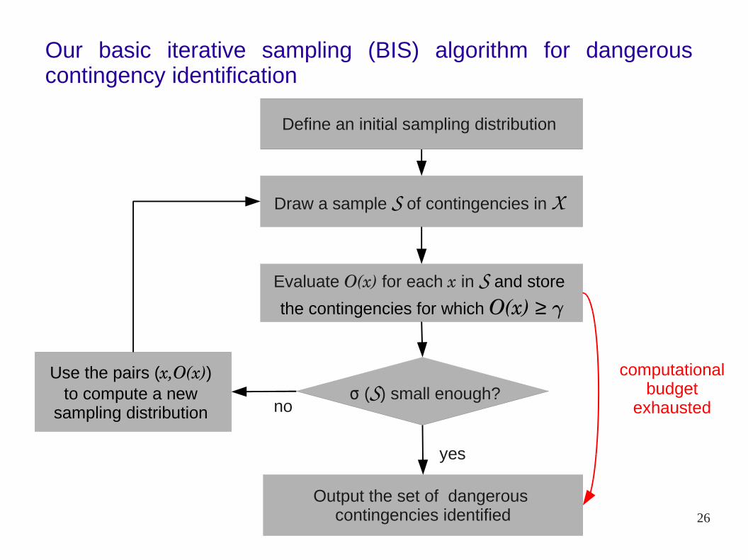
Our basic iterative sampling (BIS) algorithm for dangerous contingency identification
Draw a sample S of contingencies in X
Output the set of dangerous contingencies identified
yes
Evaluate O(x) for each x in S and store
the contingencies for which O(x) ≥ Í
Define an initial sampling distribution
Use the pairs (x,O(x)) to compute a new
sampling distribution σ (S) small enough?
no
computational budget
exhausted

27
Our comprehensive iterative sampling algorithm for dangerous contingency identification
➢ the basic iterative sampling algorithm is repeated as long as the available computational resources have not been exhausted;
2. An iterative sampling approach based on derivative-free optimization methods
Execute BIS algorithm
Computational budget
exhausted?
Output the set of different dangerous contingencies identified
yes
no

28
The objective function
➢role
- direct the sampling process towards dangerous contingencies;
➢examples
- global criteria: impact of unsupplied energy, distance of some system variables to their acceptability limits, voltage stability limits;
- equipment-based criteria: nodal voltage collapse proximity indicators, post-contingency line flows.
2. An iterative sampling approach based on derivative-free optimization methods

29
3. Embedding the contingency space in a Euclidean space
Motivation
➢ our comprehensive iterative sampling algorithm works in a Euclidean space and uses the Euclidean metric;
➢ there is no natural metric in the contingency spaces in power system security assessment problems;
=> to use this algorithm for power system security assessment,
we propose to embed the contingency space X in a Euclidean
space Y in which the algorithm is executed.

30
3. Embedding the contingency space in a Euclidean space
Metrization process, illustration
Contingency space, X Euclidean embedding space, Y(e.g., ℝ² or ℝ2k)
Projection operator

31
3. Embedding the contingency space in a Euclidean space
Metrization process, illustration
Contingency space, X Euclidean embedding space, Y(e.g., ℝ² or ℝ2k)
Projection operatorPreimage function
32
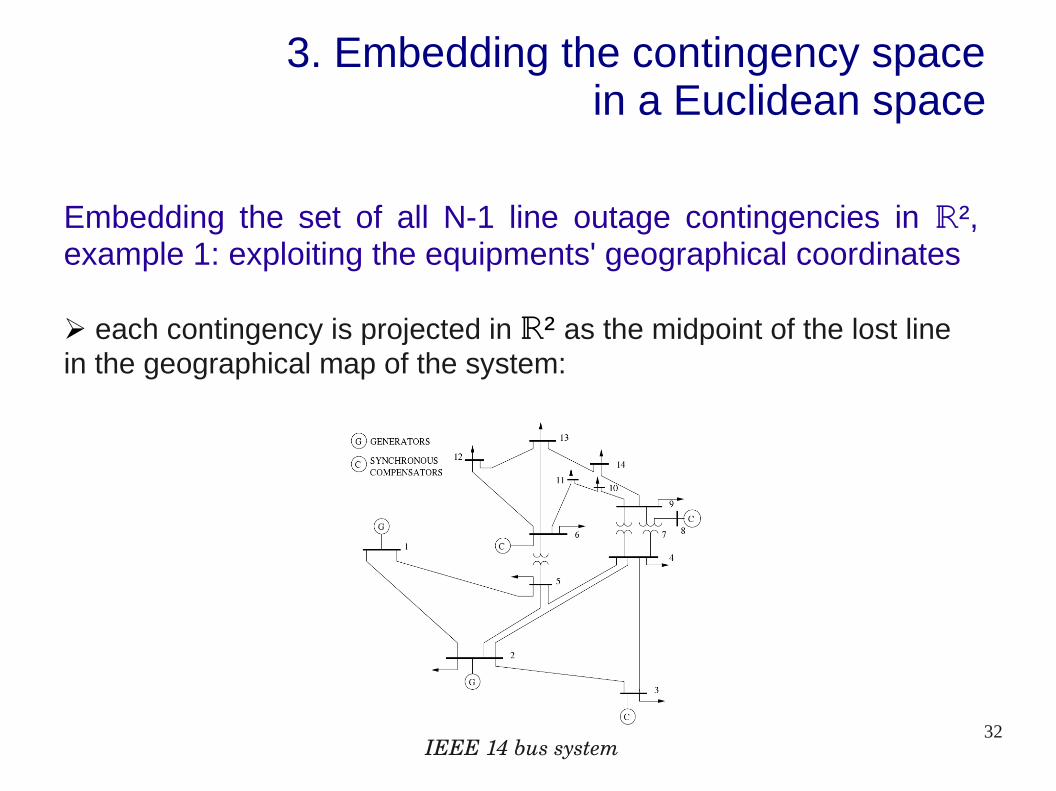
3. Embedding the contingency space in a Euclidean space
Embedding the set of all N-1 line outage contingencies in ℝ², example 1: exploiting the equipments' geographical coordinates
➢ each contingency is projected in ℝ² as the midpoint of the lost line in the geographical map of the system:
IEEE 14 bus system

33
3. Embedding the contingency space in a Euclidean space
Embedding the set of all N-1 line outage contingencies in ℝ², example 1: exploiting the equipments' geographical coordinates
➢ each contingency is projected in ℝ² as the midpoint of the lost line in the geographical map of the system:
Projection of the contingencies as the midpoints of the transmission lines

34
3. Embedding the contingency space in a Euclidean space
Embedding the set of all N-1 line outage contingencies in ℝ², example 1: exploiting the equipments' geographical coordinates
➢ the pre-image function associates to each point of the plane the projected contingency it stands the closest to:

35
3. Embedding the contingency space in a Euclidean space
Extension of example 1: embedding set of all N-k line outage contingencies in ℝ2k
➢ projection of the contingency (l1 , l
2, ..., l
i ,..., l
k):
point with coordinates (y1 , y
2 , ..., y
2i1 , y
2i , ..., y
2k),
coordinates of the midpoint of line li in the geographical
map of the system.

36
3. Embedding the contingency space in a Euclidean space
Extension of example 1: embedding set of all N-k line outage contingencies in ℝ2k
➢ pre-image of the point of coordinates (y1 , y
2 , ..., y
2i1 , y
2i , ..., y
2k):
contingency (l1 , l
2, ..., l
i ,..., l
k),
line whose midpoint is the nearest neighbor of the point with coordinates (y
2i1 , y
2i).

37
3. Embedding the contingency space in a Euclidean space
Embedding the set of all N-1 line outage contingencies in ℝ2, example 2: exploiting ''electrical'' equipment coordinates
➢ based on the electrical distances between equipments, we first compute new bus coordinates thanks to a multi-dimensional scaling algorithm;

38
3. Embedding the contingency space in a Euclidean space
Embedding the set of all N-1 line outage contingencies in ℝ2, example 2: exploiting ''electrical'' equipment coordinates
➢ each contingency is projected in ℝ² as the midpoint of the lost line in the ''electrical'' map of the system;
➢ the pre-image function also associates to a point of ℝ2 the nearest projected contingency;
➢ this procedure can be extended to the set of all N-k line outage contingencies in the same way as the previous one.
39
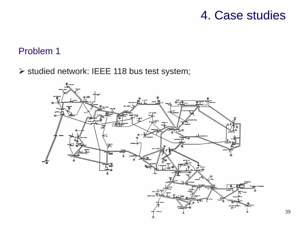
4. Case studies
Problem 1
➢ studied network: IEEE 118 bus test system;

40
4. Case studies
Problem 1
➢ contingency space: N-3 line tripping contingencies in a given base case (1 055 240 potential contingencies);
➢ objective function: number of iterations required by an AC load-flow algorithm applied to the post-contingency situation to converge;
➢ dangerous contingencies: contingencies such that O(x) ≥ 11;
➢ Euclidean embedding space: ℝ6 (electrical distances).

41
4. Case studies
Results
➢ number of contingencies screened when the first dangerous contingency is identified (our approach):

42
4. Case studies
Results
➢ number of contingencies screened when the first dangerous contingency is identified (classical Monte Carlo sampling):
43
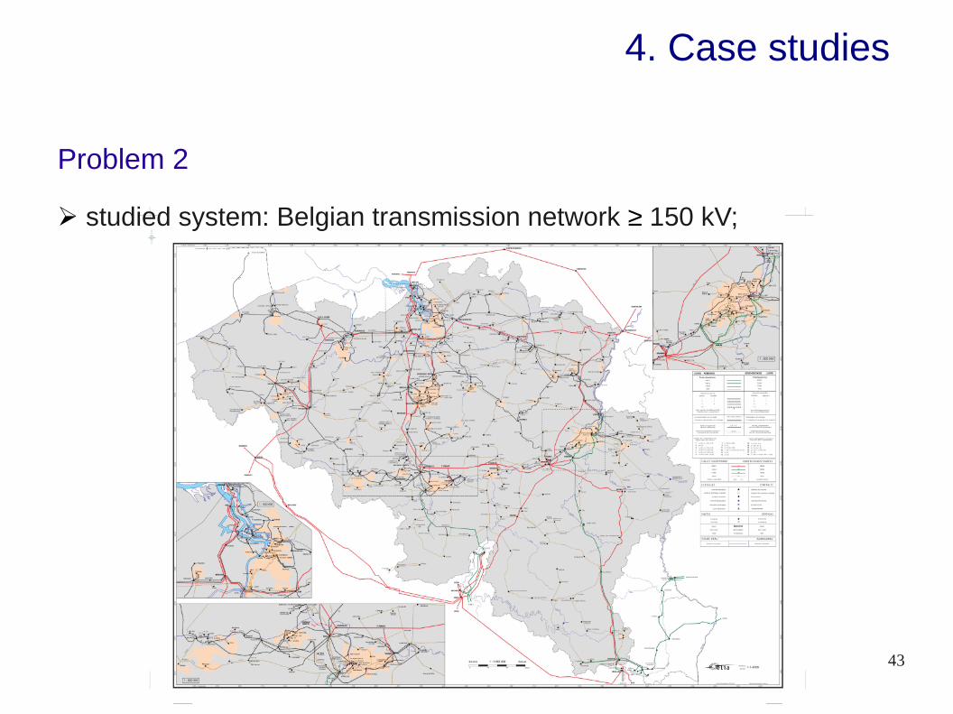
4. Case studies
Problem 2
➢ studied system: Belgian transmission network ≥ 150 kV;

44
4. Case studies
Problem 2
➢ contingency space: N-2 line tripping contingencies in a given base case (201 295 potential contingencies);
➢ objective function: maximal loading rate (in %) observed over all the lines in the post-contingency steady-state;
➢ dangerous contingencies: O(x) ≥ 170;
➢ Euclidean embedding space: ℝ4 (geographical coordinates).

45
4. Case studies
Simulation results
➢ number of dangerous contingencies identified vs available computational budget (mean and standard deviation over 100 runs):
210

46
4. Case studies
Simulation results
➢ number of dangerous contingencies identified vs available computational budget (mean and standard deviation over 100 runs):
210

47
4. Case studies
Simulation results
➢ probability of identifying at least n dangerous contingencies with a computational budget of 750 contingency analyses:

48
4. Case studies
Simulation results
➢ probability of identifying at least n dangerous contingencies with a computational budget of 750 contingency analyses:

49
5. On-line selection of iterative sampling algorithms
Context
➢ several basic iterative sampling algorithms (differing by their parameters) are available;
BIS1
(λ0
1, s1, m1)
BIS3
(λ0
3, s3, m3)
BIS4
(λ0
4, s4, m4)
BIS2
(λ0
2, s2, m2)
Probability of identification of dangerous contingencies 1 to 6

50
5. On-line selection of iterative sampling algorithms
Context
➢ several basic iterative sampling algorithms (differing by their parameters) are available;
BIS1
(λ0
1, s1, m1)
BIS3
(λ0
3, s3, m3)
BIS4
(λ0
4, s4, m4)
BIS2
(λ0
2, s2, m2)
Probability of identification of each dangerous contingency

51
5. On-line selection of iterative sampling algorithms
Objective
➢ we consider that these algorithms can be executed sequentially until the available computational resources are exhausted;
➢ we want to schedule their execution so as to maximize the number of dangerous contingencies identified.
BIS ? BIS ?BIS ? ...
Computational resources exhausted
Step 1 Step 2 Step t

52
5. On-line selection of iterative sampling algorithms
Proposed strategy
➢ a discovery rate-based strategy, scoring at each step the different algorithms according to their ability to discover new dangerous contingencies and selecting the one with the highest score;
Definition of the discovery rate: number of new dangerous contingencies identified over the last T runs of algorithm i.
➢ this strategy is compared to a strategy looping over the series of algorithms at hand.

53
5. On-line selection of iterative sampling algorithms
Simulation results: studied problem
➢ considered system: Belgian transmission system ≥ 150 kV;
➢ contingency space: N-1 line tripping contingencies in a given base case (634 potential contingencies);
➢ objective function: loading rate (in %) induced on one specific transmission line, the line Ruien-Wortegem 150 kV;
➢ dangerous contingencies: O(x) ≥ 100;
➢ Euclidean embedding space: ℝ2 (geographical coordinates).

54
5. On-line selection of iterative sampling algorithms
Simulation results: studied problem
➢ projection of the N-1 contingencies in ℝ2 (in blue) and dangerous contingencies (in red);

55
5. On-line selection of iterative sampling algorithms
Simulation results: studied problem
➢ set of BIS algorithms at hand: 9 different algorithms initialized in the 9 areas delimited in black on the picture;

56
5. On-line selection of iterative sampling algorithms
Simulation results
➢ number of different dangerous contingencies identified by the two selection strategies with increasing computational budgets;

57
6. Estimating the probability and cardinality of the set of dangerous contingencies
Main ideas
➢ we focus here on discrete contingency spaces, in which we consider that all contingencies are uniformly distributed (with probability p);
➢ we use our basic iterative sampling algorithm and exploit the principle of the cross-entropy method for rare-event simulation so as to estimate the probability l of the event {O(x) ≥ Í}:
;
➢ we also propose to derive from this latter probability an estimation of the cardinality n
dang of the set of dangerous contingencies:

58
6. Estimating the probability and cardinality of the set of dangerous contingencies
Simulation results
➢ considered problem: N-2 analysis of the Belgian transmission network, as in section 4;
(objective function: maximal overload induced on the lines of the system, Í = 170, contingency space embedded in ℝ4 using the equipments' geographical coordinates);
➢ results obtained after 100 runs of our BIS algorithm and of a naive Monte Carlo sampling algorithm:

59
7. Conclusion and future work
We have proposed in this thesis to apply iterative sampling techniques to the field of power system analysis.
Further research directions
➢ explore new variants of the proposed algorithms;
➢ integrate the developed approach to the security assessment procedures used by TSOs;
➢ extend the use of such algorithms to the control part of the security assessment task.

60
Thank you!

61