identification of desired operational spaces via numerical
TRANSCRIPT

Identification of Desired
Operational Spaces via Numerical
Methods
Prevlen Rambalee
©© UUnniivveerrssiittyy ooff PPrreettoorriiaa

Identification of Desired
Operational Spaces via Numerical
Methods
Prevlen Rambalee
©© UUnniivveerrssiittyy ooff PPrreettoorriiaa
Identification of Desired Operational Spacesvia Numerical Methods
by
Prevlen Rambalee
A dissertation submitted in partial fulfillment
of the requirements for the degree
Master of Engineering (Control Engineering)
in the
Department of Chemical Engineering
Faculty of Engineering, the Built Environment and Information
Technology
University of Pretoria
Pretoria
January 2012
©© UUnniivveerrssiittyy ooff PPrreettoorriiaa

Identification of Desired Operational Spaces via Nu-
merical Methods
Synopsis
Plant efficiency and profitability are becoming increasingly important and operating at
the most optimal point is a necessity. The definition of proper operational bounds on
output variables such as product quality, production rates etc., is critical for plant opti-
misation. The use of operational bounds that do not lie within the region of the output
operational space of the plant can result in the control system attempting to operate
the plant in a non attainable region. The use of operational bounds that lie within the
bounds of the output operational space of the plant and if the output operational space
is non convex can also result in the control system attempting to operate the plant in a
non attainable region. This results in non feasible optimisation.
A numerical intersection algorithm has been developed that identifies the feasible re-
gion of operation known as the desired operational space. This is accomplished by finding
the intersection of the required operational space and the achievable output operational
space. The algorithm was simulated and evaluated on a case study under various scenar-
ios. These scenarios included specifying operational bounds that lie partially within the
bounds of the achievable operational space and also specifying operational bounds that
lie within the bounds of the operational space which was non convex. The results yielded
a desired operational space with bounds that were guaranteed to lie within an attainable
region on the output operational space. The desired operational space bounds were also
simplified into a rectangle with high and low limits that can be readily used in control
systems.
Keywords: constraints, feasible regions, intersection algorithms, optimisation, desired
output space.
i
©© UUnniivveerrssiittyy ooff PPrreettoorriiaa

ACKNOWLEDGEMENTS
Firstly I thank the Lord for creating all the opportunities and abilities given to me. To
my late father, thank you for all the inspiration you have given to me to have the never
say die attitude. To my study leader, thanks for the direction and great ideas you have
given during this journey.
Lastly to my pillar of strength, my wife Kershnie. Thank you for all the understanding,
patience, love and laughs throughout all the long nights and weekends.
ii
©© UUnniivveerrssiittyy ooff PPrreettoorriiaa

CONTENTS
1 Introduction 1
1.1 Background . . . . . . . . . . . . . . . . . . . . . . . . . . . . . . . . . . 1
1.2 Problem Statement . . . . . . . . . . . . . . . . . . . . . . . . . . . . . . 4
1.3 Objective . . . . . . . . . . . . . . . . . . . . . . . . . . . . . . . . . . . 5
1.4 Method . . . . . . . . . . . . . . . . . . . . . . . . . . . . . . . . . . . . 8
2 Literature 11
2.1 Plant Operability . . . . . . . . . . . . . . . . . . . . . . . . . . . . . . . 11
2.2 Plant Optimisation . . . . . . . . . . . . . . . . . . . . . . . . . . . . . . 18
2.3 Optimisation . . . . . . . . . . . . . . . . . . . . . . . . . . . . . . . . . 26
2.3.1 Objective Functions . . . . . . . . . . . . . . . . . . . . . . . . . 26
2.3.2 Optimisation Techniques . . . . . . . . . . . . . . . . . . . . . . . 28
2.3.3 Uncertainty . . . . . . . . . . . . . . . . . . . . . . . . . . . . . . 30
2.3.4 Real Time Optimisation . . . . . . . . . . . . . . . . . . . . . . . 31
2.4 Process Modelling and Simulation . . . . . . . . . . . . . . . . . . . . . . 34
2.4.1 Process Modelling . . . . . . . . . . . . . . . . . . . . . . . . . . . 34
2.4.2 Simulation . . . . . . . . . . . . . . . . . . . . . . . . . . . . . . . 35
2.4.3 Simulation Results . . . . . . . . . . . . . . . . . . . . . . . . . . 35
2.5 Geometric Intersection . . . . . . . . . . . . . . . . . . . . . . . . . . . . 37
2.5.1 Two-Dimensional Intersection . . . . . . . . . . . . . . . . . . . . 37
2.5.2 Three-Dimensional Intersection . . . . . . . . . . . . . . . . . . . 42
3 Experimental 45
iii
©© UUnniivveerrssiittyy ooff PPrreettoorriiaa

3.1 Case Study . . . . . . . . . . . . . . . . . . . . . . . . . . . . . . . . . . 48
3.1.1 HCl Flash . . . . . . . . . . . . . . . . . . . . . . . . . . . . . . . 48
3.2 Modelling and Simulation . . . . . . . . . . . . . . . . . . . . . . . . . . 50
3.3 Intersection . . . . . . . . . . . . . . . . . . . . . . . . . . . . . . . . . . 52
3.3.1 Data Pre-processing . . . . . . . . . . . . . . . . . . . . . . . . . 52
3.3.2 Intersection Test . . . . . . . . . . . . . . . . . . . . . . . . . . . 55
3.3.3 Data Post Processing . . . . . . . . . . . . . . . . . . . . . . . . . 56
3.4 Key Performance Metrics (KPM) . . . . . . . . . . . . . . . . . . . . . . 60
4 Results 63
4.1 Method . . . . . . . . . . . . . . . . . . . . . . . . . . . . . . . . . . . . 63
4.2 OOS region . . . . . . . . . . . . . . . . . . . . . . . . . . . . . . . . . . 64
4.3 ROS region . . . . . . . . . . . . . . . . . . . . . . . . . . . . . . . . . . 66
4.4 DOS region . . . . . . . . . . . . . . . . . . . . . . . . . . . . . . . . . . 67
5 Discussion 72
iv
©© UUnniivveerrssiittyy ooff PPrreettoorriiaa

LIST OF FIGURES
1.1 Plant IOS and OOS regions. . . . . . . . . . . . . . . . . . . . . . . . . . 2
1.2 Plant ROS and OOS regions. . . . . . . . . . . . . . . . . . . . . . . . . 3
1.3 Various ROS and OOS region of intersections. . . . . . . . . . . . . . . . 4
1.4 Power plant heat versus power generation. . . . . . . . . . . . . . . . . . 6
1.5 Identifying plant DOS region. . . . . . . . . . . . . . . . . . . . . . . . . 7
1.6 DOS region upper and lower bounds. . . . . . . . . . . . . . . . . . . . . 8
2.1 Achievable output space of a binary mixing system. . . . . . . . . . . . . 15
2.2 Approach to plant optimisation. . . . . . . . . . . . . . . . . . . . . . . . 19
2.3 Effect of additional cooling capacity on profitability. . . . . . . . . . . . . 20
2.4 Generalised optimisation strategy. . . . . . . . . . . . . . . . . . . . . . . 25
2.5 Generalised optimisation strategy with DOS region. . . . . . . . . . . . . 27
2.6 Multilayer control structure. . . . . . . . . . . . . . . . . . . . . . . . . . 32
2.7 Identifying DOS region by geometric intersection. . . . . . . . . . . . . . 38
2.8 Convex(a) and non-convex (b and c) polygons. . . . . . . . . . . . . . . . 39
2.9 Triangulation of a polygon. . . . . . . . . . . . . . . . . . . . . . . . . . . 40
2.10 Horizontal plane sweep of polygon P. . . . . . . . . . . . . . . . . . . . . 41
3.1 Generalised approach when defining plant operational parameters. . . . . 46
3.2 Generalised approach when defining plant operational parameters using
the DOS region. . . . . . . . . . . . . . . . . . . . . . . . . . . . . . . . . 47
3.3 HCl FLASH circuit. . . . . . . . . . . . . . . . . . . . . . . . . . . . . . . 49
3.4 Data flow of simulating the process model. . . . . . . . . . . . . . . . . . 52
3.5 OOS data from simulating a model. . . . . . . . . . . . . . . . . . . . . . 53
v
©© UUnniivveerrssiittyy ooff PPrreettoorriiaa

3.6 Normalised meshed OOS data. . . . . . . . . . . . . . . . . . . . . . . . . 54
3.7 Simulation OOS data normalisation flow. . . . . . . . . . . . . . . . . . . 54
3.8 ROS data normalisation flow. . . . . . . . . . . . . . . . . . . . . . . . . 55
3.9 Summation of OOS and ROS matrices. . . . . . . . . . . . . . . . . . . . 56
3.10 Left right plane sweep of intersected matrix. . . . . . . . . . . . . . . . . 57
3.11 Identifying optimised rectangles from plane sweep matrix. . . . . . . . . 57
3.12 Post processing data flow. . . . . . . . . . . . . . . . . . . . . . . . . . . 58
3.13 Summary data flow to identify DOS region. . . . . . . . . . . . . . . . . 59
4.1 OOS region for Flash Solvent Flow versus Bottom HCL Flow. . . . . . . 65
4.2 OOS region for Flash HCL Flow versus Bottom HCL Flow. . . . . . . . . 65
4.3 DOS regions for Flash HCL Flow versus Bottom HCL Flow ROS. . . . . 68
4.4 DOS rectangles for ROS parameter Set 2. . . . . . . . . . . . . . . . . . 69
4.5 DOS rectangles for ROS parameter Set 3. . . . . . . . . . . . . . . . . . 71
vi
©© UUnniivveerrssiittyy ooff PPrreettoorriiaa

LIST OF TABLES
3.1 HCL flash process operational specifications. . . . . . . . . . . . . . . . . 50
3.2 Final DOS parameters. . . . . . . . . . . . . . . . . . . . . . . . . . . . . 58
4.1 HCl process Input Operational Space. . . . . . . . . . . . . . . . . . . . . 64
4.2 HCl process Available Output Space. . . . . . . . . . . . . . . . . . . . . 64
4.3 ROS parameters Set 1. . . . . . . . . . . . . . . . . . . . . . . . . . . . . 67
4.4 DOS parameters Set 1 . . . . . . . . . . . . . . . . . . . . . . . . . . . . 67
4.5 DOS optimised parameters Set 2. . . . . . . . . . . . . . . . . . . . . . . 70
4.6 DOS parameters Set 2. . . . . . . . . . . . . . . . . . . . . . . . . . . . . 70
vii
©© UUnniivveerrssiittyy ooff PPrreettoorriiaa

NOMENCLATURE
Acronyms
DOS Desired Operational Space
HCl Hydrochloric Acid
IOS Input Operational Space
KPM Key Performance Metric
Max Maximum Value
Min Minimum Value
MPC Model Predictive Control
OCI Output Controllability Index
OOS Output Operational Space
ROS Required Operational Space
RTO Real Time Optimisation
Symbols
Bs Bin Size
G Plant Model
viii
©© UUnniivveerrssiittyy ooff PPrreettoorriiaa

No Number
R Matrix Size
X Input Variable Matrix
Y Output Variable Matrix
∩ intersected with
⊃ super set
/∈ not an element
� Feasible Region
�̃ Non Feasible Region
� Utilisation of a Region
� Time in seconds
� Representing a function
Subscripts
l Lower bound of variable
u Upper bound of variable
i Element of matrix
n Normalised value
ix
©© UUnniivveerrssiittyy ooff PPrreettoorriiaa

CHAPTER 1
INTRODUCTION
1.1 Background
The ability of a plant to operate efficiently and on desired specifications is becoming
increasingly important. The global competitive market requires cost effective, quality
products therefore production facilities around the world are constantly optimising pro-
cesses. Optimisation of a plant involves gaining maximum utilisation of current equipment
while being safe and economically efficient. This requires identifying bounds for key plant
output parameters and operating within desired bounds. These output parameters are
typically measurements such as product quality, temperatures, product flows etc. The
output parameters of the plant are a function of and limited by input parameters, such
as valve positions, pump speeds, etc. The bounds on the input parameters can be a
result of various factors such as physical equipment limitations, safety constraints etc.
These bounds define a region known as the input operational space, IOS, of the plant.
Simulating the IOS in a steady state model of the plant will result in output parameters
forming a region known as the output operational space, OOS. This is illustrated using
a two input, two output plant in Figure 1.1;
The inputs, X1 and X2, in Figure 1.1.(a), form the IOS, where the constraints on the
input variables are;
X1l < X1 < X1u (1.1)
where X1l and X1u are lower and upper bounds of input X1.
1
©© UUnniivveerrssiittyy ooff PPrreettoorriiaa

CHAPTER 1. INTRODUCTION 2
IOS
X2U
X2L
X1L X1U
X1
X2
Plant
Model = X
Y1
Y2 OOS
(a) (b) (c)
Figure 1.1: Plant IOS and OOS regions.
X2l < X2 < X2u (1.2)
where X2l and X2u are lower and upper bounds of input X2.
Simulation of the steady state plant model with inputs within the constraints of the
IOS generates the OOS region. The OOS region is generated as follows;
OOS = G(X) (1.3)
where G represents a linear plant model in Figure 1.1.(b), as a function of the IOS
parameters. The plant model, G, is representative of a linear systems as in nonlinear
systems, the input space may not map the output space in some non linear systems as
one set of inputs may have more than one associated output points and the above OOS
region would not be valid.
The outputs, Y1 and Y2, in Figure 1.1.(c), form the OOS. The OOS region has an
irregular shape and includes a region within the boundaries that is non attainable. Op-
erational bounds on outputs Y1 and Y2 due to requirements such as production, product
quality, economics, down or up stream requirements form the region known as the re-
©© UUnniivveerrssiittyy ooff PPrreettoorriiaa

CHAPTER 1. INTRODUCTION 3
quired operational space, ROS and typically the ROS region is defined by upper and
lower bounds. In Figure 1.2, a ROS region is superimposed on the OOS region identified
in Figure 1.1.(c);
Y1
Y2 OOS ROS
YR1L YR1U
YR2U
YR2L
Figure 1.2: Plant ROS and OOS regions.
The ROS region bounds, for outputs, Y1 and Y2, in Figure 1.2, are as follows;
Y1Rl < Y1 < Y1Ru (1.4)
where Y1Rl and Y1Ru are lower and upper bounds of output Y1.
Y2Rl < Y2 < Y2Ru (1.5)
where Y2Rl and Y2Ru are lower and upper bounds of output Y2.
It is desirable to operate the plant within bounds such that OOS ∩ ROS. The ROS
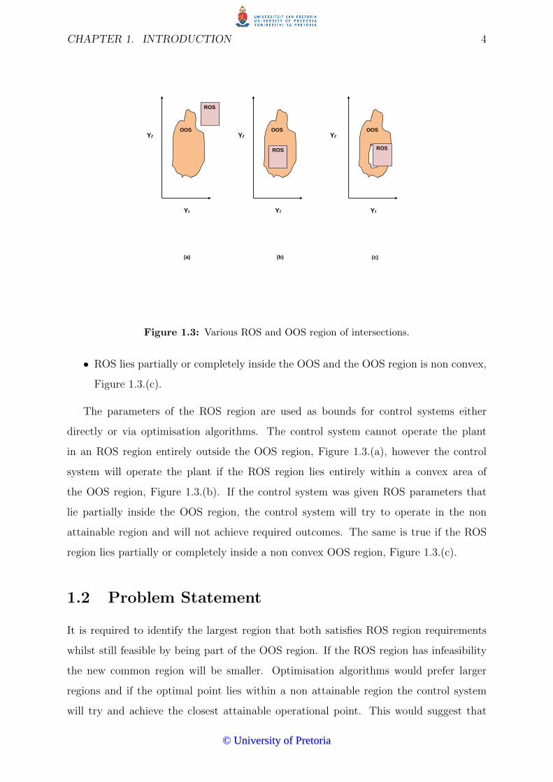
region can lie in one of three areas regarding the OOS region as shown in Figure 1.3,
In Figure 1.3 the regions can be described as follows:
• ROS lies entirely outside the OOS, Figure 1.3.(a).
• ROS lies partially or completely inside the OOS and the OOS is convex, Fig-
ure 1.3.(b).
©© UUnniivveerrssiittyy ooff PPrreettoorriiaa
CHAPTER 1. INTRODUCTION 4
Y1
Y2 OOS
ROS
Y1
Y2 OOS
Y1
Y2 OOS
(a) (b) (c)
ROS
ROS
Figure 1.3: Various ROS and OOS region of intersections.
• ROS lies partially or completely inside the OOS and the OOS region is non convex,
Figure 1.3.(c).
The parameters of the ROS region are used as bounds for control systems either
directly or via optimisation algorithms. The control system cannot operate the plant
in an ROS region entirely outside the OOS region, Figure 1.3.(a), however the control
system will operate the plant if the ROS region lies entirely within a convex area of
the OOS region, Figure 1.3.(b). If the control system was given ROS parameters that
lie partially inside the OOS region, the control system will try to operate in the non
attainable region and will not achieve required outcomes. The same is true if the ROS
region lies partially or completely inside a non convex OOS region, Figure 1.3.(c).
1.2 Problem Statement
It is required to identify the largest region that both satisfies ROS region requirements
whilst still feasible by being part of the OOS region. If the ROS region has infeasibility
the new common region will be smaller. Optimisation algorithms would prefer larger
regions and if the optimal point lies within a non attainable region the control system
will try and achieve the closest attainable operational point. This would suggest that
©© UUnniivveerrssiittyy ooff PPrreettoorriiaa

CHAPTER 1. INTRODUCTION 5
finding a region that is attainable both in the ROS and OOS region has very little value
apart from giving the control system achievable limits. However if the ROS bounds of
operation are non attainable and these bounds are used in optimisation for deliverable’s
such as production rates, quality, etc., unrealistic expectations are made and this can
severely affect operations and profitability. A motivating case study by Makkonen &
Lahdelma (2003) on the optimisation of a non convex power generation unit highlights
the need for optimisation bounds that accurately represent the process. The European
electricity market has changed to smaller competing power generating companies as op-
posed to previously large monopolised companies. These companies must now optimise
processes to meet hourly spot market variations and adhere to emission regulations whilst
realising maximum profitability under this competitive environment. These power plant
feed costs, electricity prices, electricity demand are extremely volatile such that produc-
tion optimisation and planning is based on the spot price and short term forward prices.
There are also penalties associated for slack and surplus energy production. Makkonen
& Lahdelma (2003) considered a combined power and heat plant which comprised of a
boiler, a back pressure turbine with an optional reduction bypass, condensing operation
and auxiliary cooling.
The OOS region for the combined power plant is shown in Figure 1.4. Areas two
and three are only available if the auxiliary cooling circuit is operating. The auxiliary
cooling circuit enables the plant to produce more power. If the auxiliary cooling circuit is
not operational, part of the ROS shown in Figure 1.4 is unattainable. This can result in
optimisation requiring a specific power output that the control system cannot achieve and
will result in sub optimal operation leading loss in revenue due to penalties or increased
operational costs. Therefore finding the largest feasible region between the ROS and OOS
region is sometimes required.
1.3 Objective
Optimisation algorithms including advanced controls require constraints on plant pa-
rameters to operate the plant within the desired regions. Incorrect definition of these
constraint parameters could result in the optimisation requiring the control system to
operate the plant in an unattainable region. As shown in Figure 1.1 a simulation of the
©© UUnniivveerrssiittyy ooff PPrreettoorriiaa

CHAPTER 1. INTRODUCTION 6
Power
Heat
AREA3
AREA1
AREA2
ROS
Figure 1.4: Power plant heat versus power generation.
©© UUnniivveerrssiittyy ooff PPrreettoorriiaa

CHAPTER 1. INTRODUCTION 7
plant model with the IOS constraints can be used to identify the OOS region. The con-
straints that define the ROS region can originate from various sources and as shown in
Figure 1.3 may not necessarily lie within the OOS region. This can be overcome by iden-
tifying a region known as the desired output space, DOS. The DOS is the common region
between the ROS and the OOS and is determined by finding the geometric intersection
of the OOS and ROS regions. The DOS is defined as follows;
DOS = OOS ∩ROS (1.6)
The resulting DOS region is illustrated in Figure 1.5;
Y1
Y2 OOS
ROS
DOS
Figure 1.5: Identifying plant DOS region.
In Figure 1.5 the ROS region is positioned within non attainable parts of the OOS
region. The DOS region, represented by the green shaded area in Figure 1.5, finds the
region such that equation 1.6 is satisfied. The DOS region can also be irregular in shape
which could prove difficult for control systems that require upper and lower bounds of
operation. This can be overcome by finding the largest set of upper and lower bounds
within the DOS region, as depicted in Figure 1.6;
©© UUnniivveerrssiittyy ooff PPrreettoorriiaa

CHAPTER 1. INTRODUCTION 8
Y1
Y2 OOS
ROS DOS
YD1L
YD2L
YD2U
YD1U
Figure 1.6: DOS region upper and lower bounds.
The DOS region bounds, for outputs, Y1 and Y2, in Figure 1.6, are as follows;
Y1Dl < Y1 < Y1Du (1.7)
where Y1Dl and Y1Du are lower and upper bounds of output Y1.
Y2Dl < Y2 < Y2Du (1.8)
where Y2Dl and Y2Du are lower and upper bounds of output Y2.
The objective of this study is to develop a method of identifying the DOS region via
numerical methods.
1.4 Method
To achieve the objective of identifying the DOS region via numerical methods, the fol-
lowing approach was used in this study;
©© UUnniivveerrssiittyy ooff PPrreettoorriiaa

CHAPTER 1. INTRODUCTION 9
Literature Review
The literature review study was approached as follows;
• Review previous controllability assessments methods that have been developed.
Identify the shortcomings of previous work in relation to the identification of the
DOS region, this is accomplished via a gap analysis.
• A feasible DOS regions is mainly required for plant optimisation therefore ap-
proaches to plant optimisation in different industries were reviewed. Common key
aspects are summarised to form a generic approach to plant optimisation.
• Concepts around optimisation are reviewed in further detail, this includes objective
functions, optimisation techniques, uncertainty and real time optimisation.
• Based on the above analysis of optimisation approaches, developing the DOS region
requires modelling and simulating the plant. The different methods of process
simulation are reviewed and important aspects of simulating this process model are
discussed.
• This study proposes the identification of the DOS regions via numerical methods
by reviewing geometric intersection and analysing various techniques that were
previously developed.
Experimental
Based on the information analysed in the literature review the algorithm was developed
and tested on a case study in the following manner;
• A HCL flash system was chosen as the case study. The parameters and specifications
of the circuit are specified.
• The case study was modelled and simulated based on the analysis of the literature
study.
• The simulation provided results to allow the intersection test. The data was pre-
processed to increase efficiency of the intersection as identified in the literature
study.
©© UUnniivveerrssiittyy ooff PPrreettoorriiaa
CHAPTER 1. INTRODUCTION 10
• Post processing of the intersection algorithm.
• Key performance metrics are defined to evaluate the success of the proposed tech-
nique.
Results
The proposed algorithm to numerically identify the DOS was tested and evaluated on
the case study as follows;
• The simulated case study was analysed i.e. the OOS region.
• Three sets of ROS regions were used to evaluate the intersection algorithm. The
ROS parameters included a feasible region, partially feasible region and a non con-
vex region.
• For each of the above parameter sets the results were evaluated in accordance to
the key performance metrics defined.
Discussion
The discussion summarises the approach to numerically identify the DOS region and
includes the results obtained through the case study and recommendations for future
work are discussed.
©© UUnniivveerrssiittyy ooff PPrreettoorriiaa

CHAPTER 2
LITERATURE
The literature review for this study reviews plant operability, optimisation approaches in
industries, principles of optimisation and geometric intersections.
2.1 Plant Operability
Prior to optimising a plant it is required to identify if the process is operable and con-
trollable within the bounds defined by the DOS region. A process is defined as operable
(Georgakis et al, 2003) if in the presence of disturbances and without violating any pro-
cess constraints, the desired steady state and dynamic performance of the process are
met with the available IOS. A process is defined as controllable if the ability of the IOS
keeps the process under steady state conditions in the presence of disturbances.
Several controllability assessment methods have been developed over the past three
decades. This section will review these methods and highlight the differences in their
applicability through a GAP analysis. The controllability assessment techniques include
the following:
• Time Domain analysis (Kuo & Golnaraghi, 2003 233-317).
• The use of open loop frequency response characteristics by the use of Bode and
Nyquist criterion (Seborg, Edgar & Mellichamp, 2004 376-383).
• The measure of resiliency using the Morari Resiliency Index (Lyuben,1990 573-575).
• Relative gain arrays, RGA, to determine multi-variable interaction (Marlin, 2000
334-337).
11
©© UUnniivveerrssiittyy ooff PPrreettoorriiaa

CHAPTER 2. LITERATURE 12
• Singular value decomposition with the use of condition number (Skogestad & Postleth-
waiteet, 1996 66-69).
• Steady State Feasibility using the Output controllability Index (Georgakis et al,
(2003)).
The above analysis techniques aid in the understanding of the process operability. The
first three techniques are commonly used on single input single output analysis whereby
the latter three techniques are used in multivariate analysis.
Time Domain Analysis
Involves evaluating the system’s responses with respect to time. A reference signal is
applied to the system and the performance of the system is evaluated by its time response.
Typically a unit step signal is used as an input for time response evaluations. The
following parameters are evaluated with regards to time domain analysis:
• Maximum overshoot: this is the difference between the maximum output and steady
state value. Maximum overshoot is used to measure relative stability of the control
system; a large maximum overshoot is usually undesirable.
• Time Delay: time required for the step response to reach 50% of its final value.
• Rise time: time required for the step response to rise from 10% to 90% of its
final value. The quicker the rise time the more likely the system will suffer from
overshoot. Similarly a slow rise time will result in the system taking an extended
period to reach steady state.
• Steady state error: discrepancy between the output and the reference input signal
when steady state is reached.
The above parameters are useful in evaluating and design control systems. The sta-
bility and performance of the system can be determined by analysing the time domain
characteristics.
©© UUnniivveerrssiittyy ooff PPrreettoorriiaa

CHAPTER 2. LITERATURE 13
Frequency Domain Analysis
Frequency Domain Analysis is a graphical method and it indicates how the output re-
sponse characteristic of a system depends on the frequency of the input signal. The
frequency response characteristics are calculated from the transfer function of the linear
process. Typically a sinusoidal input is used to obtain the frequency response which is
represented graphically via techniques such as the Bode and Nyquist diagrams.
Bode: Bode diagrams provide information about the amplitude ratio and phase angle
of the system as a function of frequency i.e. amplitude ratio vs. frequency and phase
vs. frequency. The amplitude ratio is defined as the ratio of the output magnitude over
the input magnitude and the phase angle is the phase difference between the input and
output signal. A critical frequency is defined whereby the phase of the system = -180
degC and the gain crossover frequency is defined when the gain =1. The control system
will become unstable if it operates at frequencies above the critical or crossover frequency.
The Bode analysis provides information about the control system stability and design.
Nyquist: Provides a polar plot of the gain and phase of the system. A Nyquist
diagram can be constructed directly from the gain and phase of the system for different
frequencies. The Nyquist plot uses the point (-1,0) and the number of times the plot
encircles this point. The Nqyuist plot can be used to analyse the stability of control
systems and can also be used for the design of control systems to ensure the process is
stable.
Morari Resiliency Index
The MRI gives an indication of the inherent controllability of a process. It is based on
the relationship between how invertible the transfer function matrix of a system is and
its resilience. The MRI is defined as the minimum singular value of the process. The
larger the minimum singular value the easier the plant is to control. This is based on
the fact that every controller tries to invert the plant directly or indirectly to find the
suitable inputs that will keep the plant at its set point. According to the MRI there are
four fundamental factors preventing the inversion of the process. These include right-
half-plane zeros, time delays, constraints on the input variables, and model uncertainty.
©© UUnniivveerrssiittyy ooff PPrreettoorriiaa

CHAPTER 2. LITERATURE 14
Relative Gain Array
In multivariate systems there are several single loop controllers which have interaction
whereby a process input affects more than one process output. Therefore the range and
controllability of multivariate systems are influenced by process interactions. This range
defines an operating window for the feasible steady state process variables that can be
achieved with the available equipment. A quantitative measure interaction is known as
the relative gain array, RGA. The RGA is a matrix composed of elements defined as
ratios of open loop to closed loop gains i.e. a matrix of relative gains. The analysis of
RGA’s can be used to pair input and output variables for control system designs and large
RGA elements indicate the plant is difficult to control due to interaction or sensitivity to
uncertainty.
Singular Values
Directions in multivariate systems are important as it provides information about the
system gains. Singular value decomposition of the system indicates the input direction,
output directions and the singular values. The singular values indicate the strongest and
weakest directions of the process. This identifies which direction the plant is more easily
controllable. The system condition number is another analysis which provide information
about the system controllability. The condition number is the ratio between the maximum
and minimum singular values. A large condition number will indicate controllability
problems.
Output Controllability Index
A technique presented by Vinson & Georgakis (2000) is a steady state controllability
measure called the output controllability index, OCI, which determines the steady state
feasibility of the ROS region based on the OOS region. The OCI uses the plant input-
output relationship to determine the limited range the input has on achieving the ob-
jectives of the process. The OCI is intended to be a single number to evaluate process
controllability and operability. The OCI is defined as follows;
OCI = �(OOSR
OS)/�(ROS) (2.1)
©© UUnniivveerrssiittyy ooff PPrreettoorriiaa

CHAPTER 2. LITERATURE 15
where � represents a function calculating the size of the space for example, in two
dimensions, it represents the area, and in three dimensions, it represents the volume. If
the OOS space is not large enough to cover the ROS space then the controllability of the
process is less than a 100 % thus resulting in a OCI less than 100%. This would imply
the IOS would require to be extended to allow the ROS region to be controllable over
the OOS region. For illustration, let us consider a continuous process where two (binary)
streams of different compositions are mixed. The input variables in the problem are the
two feed stream flow rates, F1 and F2. The outputs of interest are the product flow rate
F and its composition x: The OOS shown in Figure 2.1 is derived from the IOS given in
the in set of the same figure. If the OOS calculated is compared with DOS and the OI is
less than 1, the IOS is not sufficiently large enough to deliver all the outputs in ROS.
Figure 2.1: Achievable output space of a binary mixing system.
Georgakis et al (2003) have evaluated the OCI with other controllability measures
such as RGA, singular value, condition number, etc., and have demonstrated that the
OCI is superior to the compared techniques. The OCI highlights aspects of the process
design which require to be changed thus making a useful tool during initial process design.
©© UUnniivveerrssiittyy ooff PPrreettoorriiaa

CHAPTER 2. LITERATURE 16
In the case of an existing plant where process design changes are not always possible the
OCI does not identify the bounds of a feasible region of operation such as the DOS
region. The OCI provides open loop feasibility of both linear and non linear processes.
In industry non-linear processes are generally controlled using linear controllers, Sentosa,
Bao & Lee (2009) have proposed a technique to evaluate whether a steady state region
within the non linear process is attainable using linear feedback control. The technique
defines the largest set of initial steady-state operating points in the IOS from which the
closed loop system with linear control is guaranteed to converge to the feasible steady-
state within OOS region. It was noted that the results are only theoretical and cannot
be readily used in practise.
Other methods that have been developed on operability include (Georgakis et al,
2003):
• Swartz (1996) presented a computational framework for plant operability assess-
ment. The formulation takes the form of a convex optimisation problem and utilises
Q-parametrisation to search over all stabilising linear feedback controllers. The
solution obtained represents an upper bound on the performance of all linear sta-
bilising feedback controllers.
• Another class of operability tools and measures are those that utilise nonlinear mod-
els. The concept of a flexibility index was introduced by Swaney and Grossmann
(1985a) for quantifying the steady-state operability of nonlinear processes. This is
defined as the maximum normalized uncertainty in its parameters that a process
can tolerate without violating any constraints.
• Bahri, Bandoni, and Romagnoli (1996) formulated an optimisation-based approach
for making sure that the plant is operable in the presence of disturbances. They
moved the nominal operating point away from the constraints so that the con-
straints would not become active even when disturbances enter the plant. If the
objective function is given in terms of economic factors, the cost difference between
optimum point and back-off point quantifies the maximum savings that can be ob-
tained by decreasing the process variability by either reducing the magnitudes of
the disturbances or installing a control system
The above analysis techniques highlight the importance of ROS region being a feasible
©© UUnniivveerrssiittyy ooff PPrreettoorriiaa

CHAPTER 2. LITERATURE 17
part of the OOS region for the implementation of plant optimisation. Optimisation on a
plant that is not controllable or has limited operatability will provide little or no benefits.
GAP Analysis
The DOS region of intersection is defined as OOS ∩ ROS, however in the case when OOS
/∈ ROS, will result in a plant with limited operability. Fisher, Doherty & Douglas (1988)
suggested that lack of operability can be rectified by;
• Modifying plant flow sheets to include more or improved manipulated variables.
• Over-designing certain pieces of equipment to compensate for the complete range
of disturbances.
• Ignoring the optimisation of least important variables.
There have been several controllability assessment methods developed as discussed
previously hence a GAP analysis was performed to identify the areas of improvement. In
order for a plant to have the ability to operate efficiently and on desired specifications it
requires the following from a controllability assessment technique:
• The process must be controllable.
• The level of controllability must be identified.
• The design of controls system to provide stable performance when maintaining
required set points.
• Identify available spaces of operation for optimisation algorithms.
• Provide bounds of operation for optimisation algorithms.
Time domain and frequency domain analysis will address process controllability, level
of controllability and provide required information for the control system design. These
analyses are typically used for SISO control systems and do not address optimisation.
The MRI, RGA and singular will address process controllability and the level of
controllability. These analyses can be used on multivariate systems however do not
address optimisation.
©© UUnniivveerrssiittyy ooff PPrreettoorriiaa
CHAPTER 2. LITERATURE 18
The OCI index does address optimisation and does not analyse control system stability
or control system design. It however does identify the available achievable output space
and the limitations of the plant input variables.
The time domain, frequency domain, MRI, RGA and singular values are more relevant
to control system stability and design. The OCI and other optimisation techniques are
used once the system is controllable and stable. These optimisation techniques do not
provide feasible bounds of operation. Generally plants are required to operate optimally
within bounds defined by the end user i.e. the ROS region. This ROS region defined by
the end user may not necessarily have gone through rigorous checks for feasibility. This
creates a gap as no technique identifies the DOS region based on the ROS and OOS region.
The closest analysis is the OCI which identifies the IOS regions that requires changes to
ensure the ROS is attainable within the OOS regions. All above techniques do not
explicitly provide solutions for non convex OOS operating spaces that are not feasible.
The next section will address methods and key concepts concerning plant optimisation.
2.2 Plant Optimisation
Once the process is analysed for controllability and the various analysis have been per-
formed to ensure the process control system can keep the plant stable, optimisation can
occur. Optimisation involves changing process parameters such as feed conditions, prod-
uct and utility prices as well as equipment parameters so that the economically optimal
operating conditions of the process is realised. Thus optimisation requires the continual
adjustment of the plant operating point to coincide with the economic optimum (Young,
Baker & Swart, 2004). Several methods and techniques have been used in the process of
optimising plants around the world and these techniques vary with the type of industry
and specific plant requirements. This section will review the various approaches to opti-
misation in different industries and a general optimisation methodology is summarised.
The industries reviewed and their optimisation objectives are as follows;
• Chemical - IOS Limitations (Diaz et al, 1996)
• Chemical - Environmental (Zhang, Pike & Hertwiget, 1995)
• Power - OOS Accuracy (El-Nagger, Alrashidi & Al-Othman, 2009)
©© UUnniivveerrssiittyy ooff PPrreettoorriiaa
CHAPTER 2. LITERATURE 19
• Nuclear - Efficiency (Sayyaadi & Sabzaligol, 2009)
• Mining - Throughput (Svedensten & Evertsson, 2005)
• Petrochemical - Real Time Optimisation (Van Wyk & Pope, 1991)
Economic Factors
Determine ROS
Available OOS
Optimal Operation
Current Plant
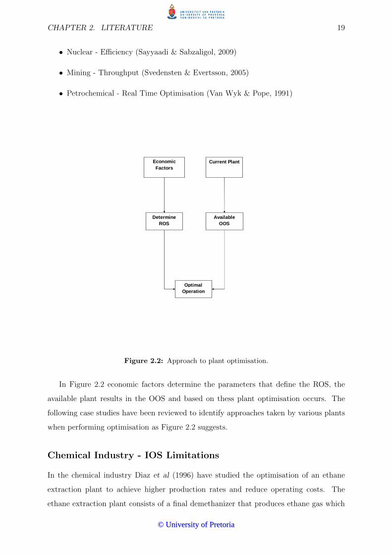
Figure 2.2: Approach to plant optimisation.
In Figure 2.2 economic factors determine the parameters that define the ROS, the
available plant results in the OOS and based on thess plant optimisation occurs. The
following case studies have been reviewed to identify approaches taken by various plants
when performing optimisation as Figure 2.2 suggests.
Chemical Industry - IOS Limitations
In the chemical industry Diaz et al (1996) have studied the optimisation of an ethane
extraction plant to achieve higher production rates and reduce operating costs. The
ethane extraction plant consists of a final demethanizer that produces ethane gas which
©© UUnniivveerrssiittyy ooff PPrreettoorriiaa

CHAPTER 2. LITERATURE 20
is compressed through three stages and delivered as sales gas. The compressors are driven
by gas turbines and form a large part of the plant operating costs. It was required to
determine if design alternatives to the current plant offer higher recoveries and lower
operating costs which would result in a better operating plant. In order to achieve this
goal a mathematical model of the current plant was built and simulated. The model
used was extended from a previous model. The simulation of the plant model included
constraints such as process specifications and bounds on equipment capacities, the IOS
region. To evaluate profitability, an economic objective function was considered in the
simulator used. The analysis indicated the optimal economic point of the plant achieves
maximum production in spite of compressor operational costs. The results have also
shown that the feed is a bottleneck to the plant. The cooling capacity of the plant was
insufficient for higher feed rates. Increasing feed rates reduces the recovery of the current
plant, thus adding additional capacity to cool the feed will result in higher production
and plant profitability. The impact of additional cooling capacity is shown in Figure 2.3
below
Figure 2.3: Effect of additional cooling capacity on profitability.
The current plant OOS does not allow for high feed rates while trying to achieve
high recoveries. If the ROS region required high feed rates the optimisation would try
to operate the current plant in a non attainable region. This case study highlights the
©© UUnniivveerrssiittyy ooff PPrreettoorriiaa

CHAPTER 2. LITERATURE 21
limitation the IOS region places on the OOS region which could cause the ROS region
to lie in a non attainable space. For the current plant using the OOS region developed
by the simulated model and the ROS, the DOS can be identified to ensure the plant will
operate in a feasible region.
Chemical Industry - Environmental
Plants around the world are also becoming more aware of their impact on the environ-
ment. Zhang, Pike & Hertwiget (1995) have implemented optimisation to reduce the
emissions of a sulphuric acid plant. The approach selected was to use a process model,
an economic model and an optimisation algorithm. The process model was developed
using a previously developed kinetic model. The process model included constraint equa-
tions such as conservation of mass and energy, reaction kinetics, equilibrium relations
and equipment operational bounds. The process model was simulated and the simulation
results, the OOS region, was compared with plant data to assess the validity and accuracy
of the process model. The economic model of the plant defined the profitability of the
plant. The process model, economic model and constraints were solved by the optimisa-
tion algorithm. Implementation of the online optimisation resulted in 25% reduction in
emissions and a 17% improvement in profit.
Power Industry - OOS Accuracy
The following case study highlights the importance of having a highly accurate OOS
region. Thermal power plant with multiple power generating units are commonly used
for providing power to the countries they serve and are an integral part of the economy.
The economic objective of these plants is to minimise fuel costs corresponding to various
generating units (El-Nagger, Alrashidi & Al-Othman, 2009). In multiple power gener-
ating units, optimal power flow and operation of each unit is important for planning
and operation. The demand for power is inconsistent and is determined by consumer
demand which can vary significantly. Producing high outputs at low demands will result
in economic losses. The estimation of the power plant heat curve, also known as the
fuel cost function curve is a key factor for optimal operation. This curve is derived from
each generating unit’s input-output characteristic hence is essentially an estimation of
the OOS region. Depending on the power demand it would be required to operate each
©© UUnniivveerrssiittyy ooff PPrreettoorriiaa

CHAPTER 2. LITERATURE 22
power generating unit at the minimum achievable cost which is based on the fuel cost
curve. In the case of the thermal power plant presented by El-Nagger et al (2009), correct
estimation of the fuel cost curve is vital for the optimisation of the plant., if the estima-
tion is not correct the optimisation algorithm will try and operate in a non attainable
region. Several methods were considered to achieve and solve the estimation:
• static estimation techniques e.g. least error square.
• dynamic estimation techniques e.g. Kalman filters.
• methods based on artificial intelligence e.g. artificial neural networks and expert
systems .
According to El-Nagger et al (2009) different algorithms produce varying levels of accu-
racy. In this case study the higher the accuracy of the estimated coefficients, the more
accurate the results for the economic operation of the power generating units.
Nuclear Industry - Efficiency
In the nuclear industry defining a ROS region without knowing the OOS region can
result in highly undesirable outcomes. Increasing profitability or throughput is only valid
if safe plant operation and adherence to legislation are achieved. The following case
study illustrates identifying the OOS region of the plant can assist in determining the
ROS region depending on the plant objective. Sayyaadi & Sabzaligol (2009) considered
a pressurised water reactor nuclear power plant for optimisation. Nuclear power plants
generally have lower efficiencies than fossil fuel plant such as the case considered by El-
Nagger et al (2009). Nuclear facilities use fuels such as uranium which are costly and not
readily available due to rarity and safety. The objective would therefore be to utilise as
much out of the nuclear fuel energy feed to the plant as possible to preserve resources.
However, it is also required to produce power in a cost effective manner. Thus there are
two different objectives for the operation of the plant. Two analyses were considered to
address each objective, the first being an economic and the second thermodynamic. To
analyse the economic performance of the plant a thermo economic model of the plant
was considered which focused on economical operation and not conservation of resources.
The thermodynamic analysis of the plant consisted of modelling based on the energy
©© UUnniivveerrssiittyy ooff PPrreettoorriiaa

CHAPTER 2. LITERATURE 23
analysis of the plant. The results showed that the thermodynamic model required more
equipment and hence a larger capital outlay but lower operational costs and vice versa
for the economic analysis. There is a tradeoff between economic versus thermal efficiency.
If the ROS is required to meet both objectives, the DOS region can be used to identify
the region which can be part of both the ROS and OOS regions.
Mining Industry - Throughput
In the mining industry, plants that process mined ore are required to be very versatile as
mined ore compositions can vary significantly which can cause the OOS region of these
plants to vary. Crushing plants are used widely in the mining industry and efficiency of
these plants severely affect profitability. The individual performance of production units
within a crusher plant affects the efficiency of the entire plant. A change in upstream
operations such as a primary crusher unit will affect the downstream production in the
plant in such a way that the quality and amount of products produced changes. Sve-
densten & Evertsson (2005) proposed a novel method for optimisation of a crusher plant
which aimed at determining the most profitable settings of the plant that maximised
profits as well as production which adhered to customer requirements. The approach
of the crusher plant included modelling the plant, feed quality, economic operation and
customer requirements. The total production of the plant was described by a plant model
such that each production unit in the crushing plant was modelled by a number of mathe-
matical models and constraints related to the specific unit. These individual models were
connected to form the crushing plant model. The feed rock material transported between
the different production units were also modelled. The rock model included parameters
such as the properties of the rock after each production unit. The economic operation of
the production costs for each production unit was modelled and the total cost comprised
of total operation costs including labour and transportation. In a crushing plant the
properties of the products produced by the crushing plant must fulfil customer demands.
This naturally places constraints on production and was included in the optimisation
process. Using the above approach the crusher plant was modelled and simulated and
the OOS region was identified. This was used to calculate the most profitable setting for
the plant.
©© UUnniivveerrssiittyy ooff PPrreettoorriiaa

CHAPTER 2. LITERATURE 24
Petrochemical Industry - On-line Optimisation
A petrochemical refinery implemented online optimisation based on a detailed mathemat-
ical model of the process and defining all potential constraints (Van Wyk & Pope, 1991)
which form the boundaries of the OOS region. The refinery planning and scheduling pro-
vides the optimisation system with economic data and quality constraints on a time scale
of days to weeks which represents the ROS region. Based on the information received by
the planning and scheduling system, the optimisation level decides the operating point
for the plant every few hours. These operating points where required to be accepted by
plant operators after which targets were downloaded to a number of advanced process
controllers. This total cycle takes about three hours. The impact on the operation of
the optimisation system was immediate; not only did the system succeed in its primary
objective of finding a more profitable operating point, but operation also became steadier
as constraints were handled more effectively. However the optimisation assumed the OOS
region was convex and the optimisation can request targets which are non feasible which
can be rejected by the plant operator. This can be solved by identifying the DOS region
and using DOS region boundaries as constraints in the optimisation.
Generalised Optimisation Strategy
The above case studies have shown that in the various applications of power genera-
tion, nuclear, chemical, mining, refinery and environmental, optimisation results in more
profitable plants whilst still adhering to specified requirements. There is a generalised
approach to process optimisation as shown in the Figure 2.4 below.
The generalised approach to optimisation shown in Figure 2.4 is as follows:
Choose Plant Area Choose an area of the plant that requires to be optimised. This
will allow input and output boundaries of the process to be defined.
Model the Plant the plant area and associated equipment.
Identify Economic Parameters Identify the various factors which influence the eco-
nomic operation of the plant.
Define Objective Function defines the objective of the chosen plant area.
Simulate Developed Model using the plant model and IOS constraints.
©© UUnniivveerrssiittyy ooff PPrreettoorriiaa

CHAPTER 2. LITERATURE 25
Start
Choose Plant Area
Identify Economic Parameters
Identify ROS
Model the Plant
Simulate developed model
Define Objective Function
Identify OOS
End
Use Optimization Algorithm
Implement Optimized Plant
Parameters
Figure 2.4: Generalised optimisation strategy.
©© UUnniivveerrssiittyy ooff PPrreettoorriiaa

CHAPTER 2. LITERATURE 26
Identify ROS is identified based on the plant requirements and economic considera-
tions.
Identify OOS is identified by the simulated model.
Use Optimisation Algorithm Once the objective function, ROS and OOS bounds are
defined, these can be used in the optimisation algorithm to solve the optimal point
of operation.
Implement Optimised Plant Parameters The output targets from the optimisation
are used as operational parameters for the plant.
The above strategy assumes the region within boundaries of the OOS is convex or
feasible. It is also not guaranteed that the ROS bounds lie within the OOS bounds or
the optimisation targets to the plant are attainable. This can be solved by determining
the DOS region as shown in Figure 2.5
The DOS region is identified by finding the feasible ROS region within the OOS
region. This will ensure that the bounds used in the optimisation will result in attainable
targets to the plant. To identify the properties the DOS should possess, each step in
the generalised optimisation approach will be reviewed in more detail in the following
sections. This includes objective functions, optimisation techniques, process modelling
and simulation.
2.3 Optimisation
The generalised optimisation approach in Figure 2.4 requires a process objective function
and an optimisation algorithm. These two aspects in addition to uncertainties faced
during optimisation and the implementation of real time optimisation will be discussed
in more detail in this sections.
2.3.1 Objective Functions
As shown in the generalised approach to optimisation in Figure 2.4, a problem statement
or objective function is required for the optimiser to solve. In order to solve constrained
optimisation objectives, the constraint variables are required (the ROS bounds and/or
©© UUnniivveerrssiittyy ooff PPrreettoorriiaa

CHAPTER 2. LITERATURE 27
Start
Choose Plant Area
Identify Economic Parameters
Identify ROS
Model the Plant
Simulate developed model
Define Objective Function
Identify OOS
End
Use Optimization Algorithm
Implement Optimized Plant
Parameters
Identify DOS
Figure 2.5: Generalised optimisation strategy with DOS region.
©© UUnniivveerrssiittyy ooff PPrreettoorriiaa

CHAPTER 2. LITERATURE 28
the OOS bounds). These constraints are grouped into economic and process constraints.
The economic constraints will include factors such as feed costs, operational costs etc.,
that are either required to be minimised or maximised. These economics are grossly af-
fected by external factors to a plant which include feed and energy costs, market demand,
price for end product, etc. The process constraints can originate either from the OOS
region that is identified by simulating a steady state process model with design param-
eters and constraints; or from the ROS which includes customer product specifications,
equipment constraints due to maintenance etc. Thereafter the objective function and
associated constraints are solved by an optimiser to determine the most profitable region
of operation. The optimisation of a process can be described by equation 2.2 (Seborg et
al, 2004 376-383);
maxF (Y1, Y2, Y3) (2.2)
subject to constraints
G(Y1, Y2, Y3) < 0 (2.3)
Hi(Y1, Y2, Y3) = 0 (2.4)
F(Y) is the objective function of the process and the constraints are defined in equa-
tions 2.3 and 2.4, which can be either equality or inequality. The inequality constraint
is represented by equation 2.3 and equality constraint represented by equation 2.4. The
optimiser is required to solve equation 2.2 whilst adhering to equations 2.3 and 2.4. Cor-
rectly defining constraints from the OOS and ROS regions is crucial for optimiser to solve
the optimisation problem.
2.3.2 Optimisation Techniques
Optimisation problems can either be constrained or unconstrained. In unconstrained
optimisation there are no inequality constraints and all equality constraints can be elimi-
nated by variable substitution in the defined objective function. Hoch & Eliceche (1999)
have shown a constrained optimisation problem in a distillation column being formulated
as unconstrained. In distillation columns the separation constraints include minimum
purity, minimum recovery and maximum impurity in a given product. For conventional
columns the operating design variables are the reflux and product flow rates. These are
©© UUnniivveerrssiittyy ooff PPrreettoorriiaa

CHAPTER 2. LITERATURE 29
two active constraints at the solution of the optimisation problem. The optimisation is
formulated as unconstrained by including the number of stages in each section of the
column as continuous optimisation variables. In the case of constrained optimisation,
the solution is bounded by specified constraints including both equality and inequality
which can either be linear or non linear. Depending on the linearity, different solutions
are required to be used to solve the optimisation problem.
Linear objective functions and linear constraints such as equations 2.3 and 2.4 can
be solved rapidly using linear programming. In the case where the objective function
is quadratic and has linear constraints, the solution can be solved in a similar fashion
as linear programming through an iterative technique known as quadratic programming
(Marlin, 2000 334-337). When the objective function or constraints are non-linear more
advanced optimisation algorithms are required to solve the optimisation problem. Opti-
misation techniques are mostly based on mathematical or stochastic methods (Beyer &
Sendhoff, 2007).
A mathematical approach can involve using modelling or programming. The model-
based methods utilise a steady state process model and programming methods include
those described above such as linear and quadratic programing. According to a survey
conducted by Beyer & Sendhoff (2007) on robust optimisation, model based methods
suffer from model mismatch uncertainty due to available measurements and the unavail-
ability of highly accurate models and mathematical optimisation algorithms such as linear
programming sometimes fail to reach a local optimum when required to solve problems
with large number of variables. A two step process which repeatedly updates uncertain
model parameters and use the updated model in the model based optimisation can be
used to address some of the drawbacks of model based optimisation (Chachuat, Marchetti
& Bonvin, 2007). This two step approach is only valid if the model mismatch is low. Since
the constraints of a model would not exactly match the plant constraints Chachuat et al
(2007) have proposed model based optimisation with a fixed process model and a con-
straint adaption algorithm that uses process measurements to update constraints. The
constraint adaption algorithm was tested on an isothermal continuous stirred reactor.
The steady state model of the process was developed from material balance equations.
The simulation results proved that the constraint adaption algorithm can also be an
alternative in addressing the drawbacks of model based optimisation.
©© UUnniivveerrssiittyy ooff PPrreettoorriiaa

CHAPTER 2. LITERATURE 30
In stochastic optimisation evolutionary algorithms are used to determine steady-state
operating periods. Evolutionary algorithms are stochastic search methods based on prin-
ciples of natural biological evolution and social behaviour of species. These techniques
include genetic algorithms, mimetic algorithms, particle swarm optimisation, ant colony
systems and shuffled frog leaping. A comparison conducted by Elbeltagi, Hagazy & Gri-
erson (2005) of the evolutionary algorithms yielded that the particle swarm optimisation
is the best.
Although most optimisation techniques are based on mathematical or stochastic meth-
ods, Li, Gu & Nui (2008) have taken a different approach to optimisation by using the
correlation analysis technique to define the operational parameters of a power plant. The
approach involved retrieving historical data, validating to remove bad data. Thereafter a
correlation analysis was performed on the cleaned operational parameters. Uncorrelated
and weakly correlation parameters were eliminated from further analysis. The relation-
ships between strongly correlated parameters were further analysed. Optimal operational
parameters settings were determined from these relationships and used as a guideline to
optimise operations.
The various optimisation techniques above have associated positive and negative at-
tributes and the technique best suited to the required application will provide the opti-
misation solution. Correctly defining the objective function and associated constraints
or bounds is important for any optimisation technique used.
2.3.3 Uncertainty
Uncertainties in the process will cause these constraints to differ from the original design
parameters. Uncertainties can be grouped into two types, aleatory and epistemic (Beyer
& Sendhoff, 2007). Aleatory uncertainties are intrinsically irreducible such as noise,
humidity, material parameters etc. These uncertainties are probabilistic in nature and
can be described mathematically. Epistemic uncertainties result from an uncertain model
used to represent the process i.e. approximations, boundary and operating conditions.
Typical uncertainties included the following (Beyer & Sendhoff, 2007);
• Changing environmental and operating conditions such as operating temperatures,
pressure and changing of material properties.
©© UUnniivveerrssiittyy ooff PPrreettoorriiaa

CHAPTER 2. LITERATURE 31
• Production tolerances and actuator imprecision, the plant production accuracy is
limited by the precision of the equipment.
• Uncertainties in the system output, due to measurement errors.
• Feasibility uncertainties that are constraints the design parameters must obey.
In a case study presented by Gao et al (2003), two MPC controllers were implemented
on the same site but on different processes namely a para-xylene unit and a propylene
splitter column. Multivariate controller performance monitoring was implemented for
these two MPC controllers and the initial benefit analysis showed improved performance
with MPC. The routine performance analysis indicated the performance on the para-
xylene unit was sustained however the propylene splitter column performance reduced.
The poor performance was largely due to model mismatch during varying load conditions
and also poor choice of constraints by operators. This finding highlights that changes in
initial plant conditions, a form of uncertainty can result in sub optimal performance and
parameters used in optimisation are required to be updated on a regular interval.
2.3.4 Real Time Optimisation
The optimisation techniques discussed can find a solution to the objective function of-
fline or online whilst the process is operational. There are advantages and disadvantages
associated with each approach. The implementation and architecture of real time opti-
misation on the petrochemical refinery has been briefly discussed by Van Wyk & Pope
(1991). The following objectives should be met when maximising the economical benefit
of an online plant and in order of importance (Tatjewski, 2008);
• Maintain the process in safe operation.
• Meet demands on product quality.
• Maximise the current production profit.
Safety of the control system is most important, once safety is achieved the control
system is required to meet demands on product quality. Once these two aims are achieved,
the process can be optimised. All the above objectives can be achieved in a multilayer
©© UUnniivveerrssiittyy ooff PPrreettoorriiaa

CHAPTER 2. LITERATURE 32
Optimizing Control
Constraint Control
Base Layer Control
Process
Measurements
Disturbances
Controlled Inputs
Figure 2.6: Multilayer control structure.
of control which can be broken up into the hierarchy shown in the Figure 2.6 (Tatjewski,
2008);
In the Figure 2.6 above, the base layer control is responsible for the basic safety of the
process and achieving sufficient stability to meet product qualities. This layer has direct
access to the plant i.e. valves, pumps, etc. The constraint layer is typically advanced
control algorithms which is used to optimise the process. The most dominant advanced
control technology is model predictive control (MPC) due to the following reasons;
• The predictive ability of MPC, it is very efficient in processes with difficult dynam-
ics.
• MPC has a unique ability to take directly into account constraints imposed on
process inputs and outputs which often have an effect on product quality and prof-
itability.
A limitation that occurs in practise is the possible infeasibility of the MPC optimisa-
tion problem due to conflicting constraints. This occurs when the ROS region does not
form part of the OOS region. The optimisation layer performs economic optimisation
related to the controlled process. The aim is to calculate the optimal steady state val-
ues for the controllers in subordinate layers. The values of the optimisation result from
©© UUnniivveerrssiittyy ooff PPrreettoorriiaa

CHAPTER 2. LITERATURE 33
the optimisation of certain objective functions typically defining profitability. Constraint
control is achieved by the use of MPC however it can also be used as an optimiser as it
allows handling of static and dynamic constraints on plant variables. Scattloini (2009)
has reviewed the architectures for MPC and the results are in agreement with the work
of Tatjewski (2008). Scattloini (2009) describes the layers of control as the base layer
having faster dynamics than the constraint layer with the optimisation layer having the
slowest dynamics. Also in a real time optimiser (RTO) the following must be considered;
• The adopted model must be updated periodically.
• Coherence must be guaranteed between the model used in the optimisation layer
and the constraint layer.
• Accurate steady state target optimisation must be done to ensure that the RTO
input and output references computed are feasible.
RTO can be defined as the online economic optimisation of a process which is based
on a steady state plant model and is only executed when the plant is stabilised and the
control problem is solved apart from the optimisation problem (Adetolai & Guay, 2010).
Thus these two layers are not necessarily dealing with the same information and the
operational point is often sub optimal. The integration of the RTO and control can be
solved by the following two techniques (Adetolai & Guay, 2010);
• The one layer approach such that the economic optimisation and control problem
are solved simultaneously in a single algorithm. Using MPC the economic objective
function can be added to the MPC objective function.
• The two layer approach involves dynamic economic optimisation and non linear
MPC. The RTO problem does not solve every sample but based on disturbance
dynamics or plant conditions. The dynamic RTO is triggered when disturbances
with high sensitivities are detected and feasible set points are recomputed.
Integration of RTO and control is still an open research problem and no theoretical
foundation such as stability and performance analysis exists.
There are drawbacks of using RTO as discussed above, however an MPC constraint
controller is sufficient to optimise the process under correctly defined constraints. Once
©© UUnniivveerrssiittyy ooff PPrreettoorriiaa

CHAPTER 2. LITERATURE 34
the DOS region is correctly identified the constraint layer such as MPC can be used to
keep the plant within these bounds.
2.4 Process Modelling and Simulation
The generalised optimisation approach in Figure 2.4 included developing a model of the
process and simulating to identify the OOS region. This section will review key concepts
regarding process modelling and simulation.
2.4.1 Process Modelling
Modelling a process requires defining the relation between inputs and outputs which can
then be used to describe the operation and behaviour of the process. There are several
techniques that can be used to model a process. Marlin (2000 426-427) has outlined the
following procedure when modelling a process;
1. Define goals of the modelling process to solve the engineering problem and the
required accuracy.
2. Identify the process, key variables and defining boundaries and assumptions.
3. Formulate the model by selecting equations based on fundamental principles.
4. Determine the format of the solution such as analytical or numerical.
5. Analyse the results by checking correctness and accuracy.
6. Validate the results by comparing with experimental results.
The first two steps in the process above are general to any modelling exercise. How-
ever, in the third step the process model can be formulated either mathematically or by
data based techniques. Mathematical models as described above by Marlin (2000 426-
427) can be used to develop process models using detailed knowledge of the physics and
chemistry of the system. Industrial processes are complex and non linear thus requiring
large effort to develop and may be subject to inaccuracies. Thus developing mathemat-
ical models of large process can become very costly. Data based modelling techniques
©© UUnniivveerrssiittyy ooff PPrreettoorriiaa

CHAPTER 2. LITERATURE 35
are alternatives to develop input-output process descriptions. There are two main cate-
gories; the first is based on statistical techniques and the second is based on the use of
artificial neural networks (McKay, Willis & Barton, 1997). Simple statistical techniques
assume that relationships between input and output variables are linear and normally
distributed. There are advanced statistical techniques to establish characteristics of non
linear process, however these techniques require a degree of expertise in interpreting these
statically based results. Neural networks are black box modelling tools which are based
on the learning of input output mappings from experimental data. Appropriate inputs
and outputs are required to be selected from the data set for the model. Usually sta-
tistical techniques are used to identify the neural network inputs and outputs. Neural
networks require large amounts of data for training and verification of the input output
mappings.
2.4.2 Simulation
Once the model of the process is developed the OOS region can be identified by simulating
the model. There exist various software modelling and simulation tools to support these
requirements. Modelling tools and simulators can be classified into two groups, block or
equation oriented (Marquardt, 1996). Block oriented approaches compromises of using
predefined blocks from a library of function blocks to model the behaviour of a process.
The parameters of the predefined blocks model can be configured to represent the process
to be modelled. These blocks are thereafter linked in a flow sheet manner to represent
the process. Equation oriented approaches involves defining mathematical equations to
model the process. Going the route of defining equations requires diverse knowledge of
various disciplines such as programming, numerical methods, chemical engineering etc.
Depending on the objective of the activity a model in being used in, different degrees of
detail in modelling will be required which can be achieved using simulation tools.
2.4.3 Simulation Results
When determining the DOS region, the objective of modelling is to identify OOS region
of the plant. In this case the format of the output of the simulated model solution is
important. Marlin (2000 426-427) postulated that the format of the output solution of the
model can be either analytical or numerical. Analytical solutions are used to determine
©© UUnniivveerrssiittyy ooff PPrreettoorriiaa

CHAPTER 2. LITERATURE 36
specific numerical values of the modelling outputs whereas in numerical solutions the
output is represented by equations. The OOS region of the plant model can be identified
using the analytical solution by varying the inputs of the model.
Rodrigues & Minceva (2005) have also summarised a generalised philosophy in process
modelling;
• Start with simple models such that the information from these models should remain
valid for complex models.
• Model validity should not be a result of good data fit but rather have the capabilities
to predict the system behaviour under operating conditions different from those used
to obtain the model.
• Good results can only be obtained if the model represents the system.
• Use the model to obtain useful design parameters and their dependency on operating
conditions.
The goal of developing a model is to predict the behaviour of the process being
modelled and to interpreting results for applications such as process design, control and
optimisation. Erroneous conclusions can be drawn from inadequate models thus building
high quality and validated models are important. Models can be validated by plant
data or experimental exercises. Collecting large amounts of data for model validation
can be resource intensive and poorly designed experiments yield little useful information.
Franceshini & Macchietto (2007) have used a technique called design of experiments.
The technique aims at obtaining the most information from experiments used to validate
models. Experimental design refers to when and how the experimenter will observe
phenomena under investigation. These observations are used to validate the model but
also to improve model parameters.
Bouchama, Sebastian & Nadeau (2003) considered a two stage flash evaporation cir-
cuit which was modelled both theoretically and experimentally. The theoretical model
was developed mathematically using fundamental thermodynamic equations. The ex-
perimental model was validated by experiments on a pilot scale model. The theoretical
model results were compared with the experimental model results. There was a difference
in the results with theoretical model being more precise but slightly inaccurate and the
©© UUnniivveerrssiittyy ooff PPrreettoorriiaa

CHAPTER 2. LITERATURE 37
resolution led to precise numerical results but was far from experimental results. The the-
oretical model parameters were fit to the experimental data using a numerical constraint
solver. The final model was used for decision support during operation.
In conclusion, modelling and simulating a process can be accomplished by a variety
of techniques but it is imperative that the modelling is representative of the process.
Developing a process model can be useful in various applications such as process design,
troubleshooting etc., however in optimisation it is required for the process model to
identify the OOS region. The simulation results of the process model can be used to
numerically determine the DOS region via intersection of the OOS and ROS region. The
next sections discusses geometric intersection.
2.5 Geometric Intersection
To optimise a process, the optimisation algorithm requires bounds on different variables
for constraint optimisation and as highlighted by Gao et al (2003), it is important to
define these limits as accurately as possible. These bounds can originate from the ROS
and or the OOS regions. As identified in the previous section simulation of the process
model will result in the identification of the plant OOS region. The output format of the
simulated model can either be analytical or numerical. An analytical output will allow the
OOS region to be represented geometrically. The ROS bounds as discussed are a function
of various factors and can also be represented geometrically. Thus intersection of these
two geometric regions would result in the desired region of operation DOS region. This
section firstly reviews two dimensional geometric intersection of polygons which includes
defining convexity and the use of triangulation. The intersection of higher dimensions
are also discussed.
In Figure 2.7, the DOS region is identified by the geometric intersection of the ROS
and OOS regions. Intersection of two-dimensional geometric regions is the basis for a
higher dimension intersection.
2.5.1 Two-Dimensional Intersection
Various techniques of two-dimensional geometric objects, polygons, intersection have been
developed. It is critical before performing any intersection tests to define the type of
©© UUnniivveerrssiittyy ooff PPrreettoorriiaa

CHAPTER 2. LITERATURE 38
Identify ROS
Identify DOS
Geometrically represent ROS
Geometrically represent OOS
Geometric Intersection
Identify OOS
Figure 2.7: Identifying DOS region by geometric intersection.
©© UUnniivveerrssiittyy ooff PPrreettoorriiaa

CHAPTER 2. LITERATURE 39
polygons that are to be used in the intersections. Polygons can grouped as either convex
or non convex as shown in Figure 2.8;
(a) (b) (c)
Figure 2.8: Convex(a) and non-convex (b and c) polygons.
In Figure 2.8 (a) a convex polygon has every internal angle less than 180 ∘ and every
line segment of the polygon remains inside the boundary of the polygon. The concave
polygon in Figure 2.8 (b) has an interior angle greater than 180 ∘. The polygon in Fig-
ure 2.8 (c) is considered non convex. When a polygon is non convex it is difficult to detect
intersection in a reasonable time without pre-processing as large amount of computational
effort is required. To improve the efficiency of geometric intersection algorithms when
dealing with non convexity, it is required to simplify the geometric shape. The most pop-
ular techniques for simplifying geometric shape of a polygon is known as triangulation.
Triangulating a polygon requires sub dividing the polygon into triangles without added
new vertices.
Figure 2.9 (a) shows a polygon which has been triangulated in Figure 2.9 (b), the
dashed lines show the triangles formed. Triangulation can become computational inten-
sive and may take a long time to accomplish, there are techniques such as fast trian-
gulation to shorten the process. Fast triangulation techniques involve inferring global
information of the polygon, which can be accomplished by either the top down or left
right up approach. The top down approach uses the polygon cutting theorem that states
©© UUnniivveerrssiittyy ooff PPrreettoorriiaa

CHAPTER 2. LITERATURE 40
(a) (b)
Figure 2.9: Triangulation of a polygon.
that the polygon can be cut along the diagonal into two equal sizes, it is however difficult
to find the diagonal. The left right approach involves computing triangulations of the
sub pieces of the polygon boundary however this requires the processing of vast amounts
of information. The solution presented by Siedel (1991) uses horizontal decomposition,
the left right approach whereby the polygon is firstly decomposed into trapezoids. This
trapezoidalization algorithm relies on the plane sweep line technique. The vertices of the
polygon P must be sorted with respect to their x-coordinates.
A vertical line, V, as shown in Figure 2.10 scans the sorted vertices and the polygon is
decomposed into trapezoids with vertical parallel edges. Once the polygon is partitioned
into simpler polygons, these polygons can easily be split into triangles by using the greedy
algorithm technique presented by O’Rouke (Narkhede & Manocha, 2010). A greedy
algorithm makes locally optimal choices with the hope of finding the global optimum.
It makes a greedy choices to reduce the problem. It is not exhaustive and does not
reconsider choices made and this can lead to a sub optimal solution.
Chazelle (1991) proposed a similar technique by using the left right approach to
build a rough approximation of the triangulation then simultaneously use the information
obtained left right approach in a top down manner to refine the triangulation.
A survey of the overview of triangulation algorithms of polygons (Lamot & Zalik,
©© UUnniivveerrssiittyy ooff PPrreettoorriiaa

CHAPTER 2. LITERATURE 41
Y
X
P
V1 V2
Figure 2.10: Horizontal plane sweep of polygon P.
1999) included various other techniques such as;
• Garey, Johnson, Preparata and Tarjan proposed a divide and conquer algorithm
which is completed in two steps. The first step decomposes simple polygon into
monotone sub-polygons and the second step triangulates these monotone sub-polygons.
• Kong, Everett and Toussaint developed an algorithm which is based on the Graham
scan. The Graham scan is a fundamental backtracking technique in computational
geometry.
• The Delaunay triangulation technique for a set P of points in the plane is a trian-
gulation such that no point in P is inside the circumcircle of any triangle. Delaunay
triangulations maximize the minimum angle of all the angles of the triangles in the
triangulation.
The above survey compared the various algorithms and concluded that the Delaunay
technique provided the highest quality and that the Siedel algorithm is the fastest. The
Siedel algorithm can also be easily modified to handle non convex polygons and is thus
©© UUnniivveerrssiittyy ooff PPrreettoorriiaa

CHAPTER 2. LITERATURE 42
the recommended algorithm for efficient triangulation.
Once the polygons are reduced either to simple polygons or triangles, the intersection
can be determined. Shamos and Hoey (O’Rouke et al, 1982) developed a technique which
determines the intersection of a pair of objects that is based on plane sweep. Each object
is bounded by an aligned box, the objects only intersect if their bounding boxes intersect.
The boxes intersect by comparing their projections on each coordinate axis. The alternate
method of determining whether the intersection exists between the triangulated objects
is to compare the vertices of the objects.
Determining the geometric intersection of polygons would involve the following;
• Identify the convexity of polygons.
• Choose a technique to simplify the polygons.
• Triangulate the simplified polygons.
• Perform an intersection test of the above triangles.
The final parameters from the intersection test will result in the DOS parameters
required in Figure 2.7. The number of output parameters in the OOS regions determines
the dimensions of the intersection, thus higher dimension intersection is discussed in the
following section.
2.5.2 Three-Dimensional Intersection
Intersection of geometric objects in a three-dimensional space is more involved than two
dimensions. Three-dimensional geometric intersection is frequently used in computer
graphics for which it is required to determine collision detection of volumes. These real
time three-dimensional intersections require efficient algorithms and a survey conducted
by Jimenez, Thomas & Torras (2001) provided an overview of various techniques de-
veloped. Most of these real time intersection techniques of three-dimensional objects
eventually require applying a static interference test between the three-dimensional poly-
hedron and similar to the intersection of polygons, convexity of the polyhedron is very
important.
Jimenez et al (2001) deduced that there are two basic contacts between two polyhedra
which reduces the interference problem in detecting edges piercing convex faces. The first
©© UUnniivveerrssiittyy ooff PPrreettoorriiaa

CHAPTER 2. LITERATURE 43
type of contact takes place when a face of one polyhedron is in contact with a vertex of
the other polyhedron and the other contact type is when an edge of one polyhedron
is in contact with an edge of the other polyhedron. Thus, most techniques decompose
the polyhedron or their boundaries into convex polyhedra. The aim is to determine the
closest points of two polyhedra, and then compute the euclidean distance between them by
using techniques such as Dobkin and Kirkpatrick’s hierarchical polyhedral representation
or the Minkowski difference of two polytopes. An alternative technique in identifying
intersection is to navigate along the boundaries of the involved polyhedra in the direction
of decreasing distance. Spherical representations are also appealing due to the simplicity
of calculating the distance between two spheres, thus ellipsoids are used to approximate
convex polyhedra. The sphere-box algorithm presented by Ratschek & Rokn (1994)
incorporates the sphere-box test as used in spatial subdivision techniques and ray tracing.
The midpoint m and the radius r are the sphere parameters. The tests determine the
smallest or largest distance from m to the box, and compare it with r. This determines
if the sphere is inside, outside or partially inside the box.
All the intersection tests for polyhedral above, similar to polygon intersection, are
dependent on the convexity of the polyhedra. A comparative study was presented by
B Chazelle et al (1997) on the techniques used to decompose the surfaces of complex
polyhedras into simpler convex surfaces. The techniques include space partitioning, space
sweeping and flooding.
• The space partitioning technique uses binary space partitioning to split up the
surface into convex patches. The method builds a tree by recursively dividing space
by a cutting plane. Each node v of the tree is associated with a convex polyhedron
Pv. The aim is to explore the two children of v if and only if the portion of the
surface within Pv is not convex.
• In the space sweep technique the cross-section of a surface consists of simple polyg-
onal curves which are decomposed into convex pieces. This technique attempts to
maintain each curve as long as possible while moving the plane, thus producing
convex patches in the process. Each time a convexity violation is found a new
convex curve is started.
• In flooding, let H be the dual graph of the surface, where nodes represent facets
©© UUnniivveerrssiittyy ooff PPrreettoorriiaa

CHAPTER 2. LITERATURE 44
and arcs join nodes associated with adjacent facets. The class of flooding heuristics
refers to the incremental strategy of starting from some node and traversing the
graph H, collecting facets along the way as long as they form a convex patch.
For the above study flooding was concluded to be the method of choice. Although it
is possible to triangulate all convex polyhedral it has been proven that it is impossible
to triangulate non convex polyhedral and little research on convex decomposition of
polyhedra has extended beyond the theoretical stage. This has proven to be a limitation
on the intersection of geometric objects in dimensions higher than two.
The literature review addressed previous controllability and optimisation methods
developed and highlighted the gap for improvement. The various industry approaches
to optimisation was reviewed and a generalised approach to optimisation was formu-
lated. Key concepts around optimisation such as objective functions, uncertainty and
real time optimisation was discussed. The generalised approach to optimisation required
the process to be modelled and simulated to identify the OOS region. The key factors for
modelling and simulation were reviewed. Identification of the DOS region requires the
intersection of the ROS and OOS feasible regions and concepts of geometric intersection
were also reviewed. The information analysed in the literature review can be used to
develop the intersection algorithm.
©© UUnniivveerrssiittyy ooff PPrreettoorriiaa

CHAPTER 3
EXPERIMENTAL
It has been established that optimisation algorithms require feasible constraints on plant
parameters to operate the plant within the desired regions. Incorrect definition of these
constraint parameters could result in the optimisation requiring the control system to
operate the plant in an unattainable region. This problem is addressed by the determining
the DOS region which is the common region between the ROS and the OOS region. The
parameters of the DOS region will provide constraints for the optimisation techniques
which will result in a feasible solution. This section reviews the case study that will
be used to evaluate the algorithm, the modelling and simulation of the case study, the
intersection algorithm and the key performance metrics required for evaluation.
There are various process plants that do not have optimisation techniques, the ap-
proach in defining plant parameters is shown in Figure 3.1;
Figure 3.1 is a simplification of the generalised optimisation approach using the DOS
region shown in Figure 2.5. The parameters for the plant are only a function of the
ROS region. The ROS region is a result of decisions that are defined by the economical
operational of the plant, factors influencing production such costs, customer requirements,
maintenance, in addition to others. These decisions are typically taken on a daily basis
by plant personnel. The bounds of the ROS region must lie within the feasible region.
Correctly defining these bounds are important as Gao et al (2003) have found that poor
choice of constraints by operators led to poor control performance. The same problem of
defining feasible operating regions is faced when using and not using optimisation. Thus
identifying the DOS region is also valid for processes that do not use optimisation as
shown in Figure 3.2;
45
©© UUnniivveerrssiittyy ooff PPrreettoorriiaa

CHAPTER 3. EXPERIMENTAL 46
Choose Plant Area
Start
Identify Economic Parameters
Identify ROS
End
Implement Plant Parameters
Figure 3.1: Generalised approach when defining plant operational parameters.
©© UUnniivveerrssiittyy ooff PPrreettoorriiaa

CHAPTER 3. EXPERIMENTAL 47
Plant Area
Start
Economic Parameters
Identify ROS
Model
Simulate
Identify OOS
End
Plant Parameters
Identify DOS
Figure 3.2: Generalised approach when defining plant operational parameters using the DOSregion.
©© UUnniivveerrssiittyy ooff PPrreettoorriiaa

CHAPTER 3. EXPERIMENTAL 48
Based on the literature and the approach shown in Figure 3.2, automatic constraint
propagation to identify the DOS region via numerical methods will involve the following
during the experimental procedure;
Identify Plant Area Identification of plants to be used as a case study.
Identify ROS region required for the above identified plant.
Model the above chosen process.
Simulate the above model.
Identify OOS from the output of the simulation.
Identify DOS by determining the intersection of the ROS and OOS regions identified.
Evaluate Results based on key performance metrics.
3.1 Case Study
An HCl flash circuit was chosen as the case study to identify the DOS region via the
proposed algorithm.
3.1.1 HCl Flash
The following process uses a flash column to flash off HCl from the available 10N HCl
feed. The feed includes the solvent, water.
The plant is designed to operate on a maximum re-boiler duty with an abundance of
feed. The feed includes a mixture of fresh 10N HCl and recycled HCl. The acid normality
and solvent content of the recycle can vary. Thus the process input variables are;
• Feed rate - kg/h.
• Feed solvent composition - mol/l.
The flash product is required to be within required specifications as determined by down-
stream processes and the bottom product is disposed as waste. The output variables of
interest are;
©© UUnniivveerrssiittyy ooff PPrreettoorriiaa
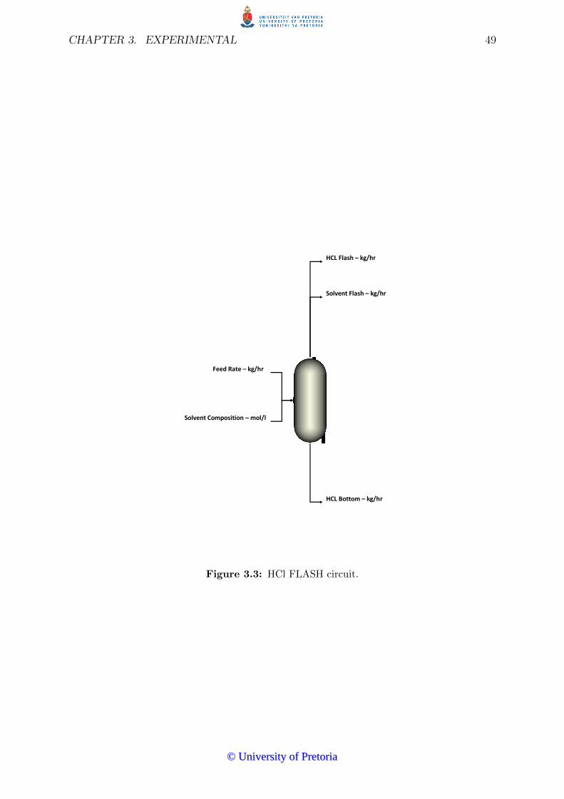
CHAPTER 3. EXPERIMENTAL 49
Feed Rate – kg/hr
Solvent Composition – mol/l
HCL Bottom – kg/hr
HCL Flash – kg/hr
Solvent Flash – kg/hr
Figure 3.3: HCl FLASH circuit.
©© UUnniivveerrssiittyy ooff PPrreettoorriiaa

CHAPTER 3. EXPERIMENTAL 50
• HCl flash product rate - kg/h .
• Solvent flash product rate - kg/h.
• HCl bottom product rate - kg/h.
The typical operating specifications of the plant are shown in Table 3.1.
Table 3.1: HCL flash process operational specifications.
Parameter Value UnitFeed Rate 5 kg/hrFeed Temperature 330.7 KFeed Composition 10 NHCLFlash Temperature 340.7 KBottom Temperature 401.7 KBottom Composition 6 NHCLOperating Pressure 117.2 kPaRe-boiler heat duty 22.4 MW
It would be required to maximise the feed rate particularly the use of recycled acid,
which would imply higher solvent composition in the feed. At the same it would also
be required to minimise HCl bottom flow rate while still being within the solvent flash
product specification.
3.2 Modelling and Simulation
In the literature survey the guideline based on Marlin (2000 334-337) when modelling
a process was discussed. The first step in modelling any process is to define the goal of
modelling, in the chosen case studies the goal is to develop a model that can be simulated
to identify the OOS region. The second step involves identifying all key process variables,
that were been identified in the detailed description of each process. The third step
requires selecting a modelling technique. There are several methods to model a process
which include modelling based on fundamental chemistry and physics or using data driven
methods. The modelling technique adopted is based on the approach illustrated by
Marquardt (1996) which incorporates block modelling tools in a simulator. The fourth
step requires determining the format of the output solution, in order to represent the
OOS region geometrically the output was numerical. The Aspen Plus Modelling toolkit
©© UUnniivveerrssiittyy ooff PPrreettoorriiaa

CHAPTER 3. EXPERIMENTAL 51
was used to model and simulate the chosen process. The following process was followed
when modelling each process in the chosen toolkit;
• The appropriate equipment was selected to best represent the system. The process
was built in a flow sheet manner by connecting various pieces of equipment to
represent the chosen process. The specifications defined in the detail description of
the process was used.
• Operational parameters defined in the detailed description of each process were
used as inputs for the various equipment and connections that made up the model.
• Key input variables were simulated by selecting variables on a rectangular mesh to
identify the effect on key output variables creating the required OOS region. Each
input variable was incremented by a fixed step size between its high and low limits.
• The simulation of the input variables via the model resulted in corresponding values
for the output variables which represented the OOS region.
Each input variable was incremented by a total number of steps, ts, between the low
and high limits. When two input variable exist, input variable one is incremented through
its entire range for each increment of the second variable. The same will apply for systems
with larger than two variables. Each increment in an input variable will result in a value
for an output variable thus the total number of data points per output variable, do, are
as follows;
do = txis (3.1)
where xi is the number of input variables incremented. Increasing the number of
steps or the number of input variables will exponentially increase the number of output
values. These increases require a more computational effort and have an impact on the
simulation time required. The converse will result in quicker simulation time however
there is a risk of losing process information due to low resolution. There is a tradeoff
between computational effort and loss of information.
The flow of data is shown in Figure 3.4, the input variables, X, are simulated which
results in output variables, Y. The output matrix Y comprises of vectors for each output
variable, i.e. the columns of Y. The matrix Y is the OOS.
©© UUnniivveerrssiittyy ooff PPrreettoorriiaa

CHAPTER 3. EXPERIMENTAL 52
X
1
.
.
.
.
.
.
.
.j
Model
Y
1...
.
.
.
.
.j
Figure 3.4: Data flow of simulating the process model.
3.3 Intersection
3.3.1 Data Pre-processing
Each output of the simulation namely is the columns of matrix Y, Yi, of the OOS region
was normalised, YN , to a range between 0 to 1. The normalised data, YN , was meshed into
an n-dimensional data structure thus the dimensionality of the data structure is based
on the number of output variables. Each dimension of the data structure are the same
size i.e. a matrix data structure will be a square. It is therefore required to specify the
size of data structure YN . Once the size of the data structure is defined the normalised
data can be meshed in the data structure, this implies that each element in YN will be
meshed into bins. Using the size of the data structure the meshing bin size, BS, can be
calculated as follows;
BS = R−1 (3.2)
where R is the size of the data structure. Similarly to equation 3.1 the larger the size
of the data structure the higher the resolution of the data however more computational
effort is required. If a normalised output value lies within a bin, the corresponding
©© UUnniivveerrssiittyy ooff PPrreettoorriiaa

CHAPTER 3. EXPERIMENTAL 53
element is set to 1. The end result is a data structure, YN such that the ones represent
the OOS region. Figure 3.5 below is an example of two output variables generated from
the simulation of the model.
Y1
Y2
20
9
26
6
Figure 3.5: OOS data from simulating a model.
In Figure 3.5 variable Y1 and Y2 range between 20 and 26, 6 and 9 respectively. The
OOS region in Figure 3.5 is represented by the dots. If the size, R, of the normalised
matrix YN was chosen to be 6, the resolution according to equation 3.2, BS is 0.166. The
meshed normalised meshed data is shown in Figure 3.6;
In Figure 3.6 the ones represent a point that is part of the OOS region. Choosing
a large size of the data structure will result in higher resolution however this is limited
to the resolution of the simulated output Y . A summary of the data pre-processing is
shown in Figure 3.7;
The normalisation of data generated by the simulation is summarised in Figure 3.7,
whereby the simulation output matrix Y is normalised and mapped to form YOOS. Sim-
ilarly the ROS bounds, YR can be represented as matrix Y and by following the same
steps, YROS can be found such that the 1’s represent the ROS. The approach shown in
Figure 3.7 can be adopted as follows;
©© UUnniivveerrssiittyy ooff PPrreettoorriiaa

CHAPTER 3. EXPERIMENTAL 54
Y1N
Y2N 0
1
1
0.33
0.66
0.33 0.66
Figure 3.6: Normalised meshed OOS data.
Define R
Indentify BS
Map YN to YOOS
Normalize
YN
1...j
YOOS
1..j
. . j
Y
1...
.
.
.
.
.
.j
Figure 3.7: Simulation OOS data normalisation flow.
©© UUnniivveerrssiittyy ooff PPrreettoorriiaa

CHAPTER 3. EXPERIMENTAL 55
Define R
Indentify BS
Map YNR to YROS
Normalize
YRN
1...j
YROS
1..j
. . j
YR
1...
.
.
.
.
.
.j
Figure 3.8: ROS data normalisation flow.
Using the approach in Figure 3.8, YROS can be determined.
3.3.2 Intersection Test
The OOS and ROS regions after pre-processing are represented by two data structures
YOOS and YROS respectively. In the case of a two output variable system, the data struc-
tures will be in the form of matrices. Identifying the DOS region involves determining the
intersection of YOOS and YROS. The literature survey has shown the most suitable geo-
metric intersection technique is presented by Chazelle (1991) which involves representing
YOOS and YROS as polygons, triangulating these polygons and finding the intersection
of these triangles. The horizontal decomposition technique presented by Siedel (1991)
can be used represent YOOS and YROS as polygons. This technique involves using plane
sweep to determine the vertices of the polygon. An alternative technique to identify the
intersection of YOOS and YROS involves finding the sum, YS of the two matrices as follows;
YS = YOOS + YROS (3.3)
The elements in YOOS and YROS are matrices consisting of 0’s and 1’s, therefore a
summation will result in intersection elements in YS having the value of 2. The DOS will
©© UUnniivveerrssiittyy ooff PPrreettoorriiaa

CHAPTER 3. EXPERIMENTAL 56
become the bounds of elements with the value of 2. This is shown in Figure 3.9;
1 1 0 0
1 1 1 0
0 1 1 0
0 0 0 0
0 0 0 0
1 1 1 1
0 1 1 1
0 0 0 0
1 1 0 0
1 2 2 1
0 2 2 1
0 0 0 0
YOOS
+ =
YROS YS
Figure 3.9: Summation of OOS and ROS matrices.
The region of intersection in Figure 3.9 is circled in red on the YS matrix. The bounds
of the region of intersection can be reconstructed by post data processing.
3.3.3 Data Post Processing
Reconstructing the region of intersection found in YS will firstly involve determining
the vertices of the intersection region boundaries. These vertices can be represented as
rectangles, therefore the horizontal decomposition technique presented by Siedel (1991)
will be used. This technique performs a left right plane sweep of the matrix. Along each
x-axis coordinate the maximum and minimum y coordinates are stored for consecutive
values of 2. This is shown by the red boxes in Figure 3.10;
Using the plane sweep technique produces rectangles, a set of y coordinates for every
sweep on each x coordinate, which can result in a large set of DOS values. In Figure 3.10
there are six rectangles and these six rectangles can be optimised and reduced. This
is accomplished by identifying larger optimised rectangles within the set of coordinates
provided by the plane sweep technique. The optimised rectangles are determined by
finding the rate of change of the x and y coordinates. If the rate of change is zero for
both the axises then those coordinates form part of the trapezoid. This is shown in
Figure 3.11;
©© UUnniivveerrssiittyy ooff PPrreettoorriiaa

CHAPTER 3. EXPERIMENTAL 57
0 1 0 0 1 1
0 1 1 0 0 0
2 2 1 0 2 2
2 2 0 0 2 2
0 0 2 2 2 2
1 1 2 2 2 2
Plane Sweep
Figure 3.10: Left right plane sweep of intersected matrix.
0 1 0 0 1 1
0 1 1 0 0 0
2 2 1 0 2 2
2 2 0 0 2 2
0 0 2 2 2 2
1 1 2 2 2 2
Figure 3.11: Identifying optimised rectangles from plane sweep matrix.
©© UUnniivveerrssiittyy ooff PPrreettoorriiaa

CHAPTER 3. EXPERIMENTAL 58
The coordinates of the optimised rectangles become the DOS, YDOS in the form shown
in Table 3.2;
Table 3.2: Final DOS parameters.
YDOSXMN YDOSXMX YDOSYMN YDOSYMX
1 2 3 43 4 1 25 6 1 4
The parameters YDOSXMN is the x axis lower bound, YDOSXMX is the x axis upper
bound, YDOSYMN is the y axis lower bound and YDOSYMX is the y axis upper bound. A
summary of the data post-processing is shown in Figure 3.12;
YS
1..
.
.
.
.
.
.
.
.
.
j
. . j
Find
Intersection
vertices –
plane sweep
Find
Rectangles
Optimize
Rectangles
YDOS
YN YX XN XM
1 10 5 6
2 3 2 8
Figure 3.12: Post processing data flow.
A summary of the approach of determining DOS from OOS and ROS region is shown
in Figure 3.13;
In Figure 3.13 the procedure is used to determine the DOS region is shown and can
be summarised as follows;
©© UUnniivveerrssiittyy ooff PPrreettoorriiaa

CHAPTER 3. EXPERIMENTAL 59
1 1 0 0 1 1 1 0 0 1 1 0 0 0 0 0
0 0 0 0 1 1 1 1 0 1 1 1 0 0 0 0
1 1 0 0 1 2 2 1 0 2 2 1 0 0 0 0
Find Intersection
vertices – plane sweep
Find Rectangles
Optimize Rectangles
YDOS
Define R
Indentify BS
Map YN to YOOS
Map YNR to YROS
YR
1...
j
YRN
1..
.j Normalize
X
1...j
Model
Y
1...
j
YN
1...
j
Normalize
YOOS YROS YS
+ =
Figure 3.13: Summary data flow to identify DOS region.
©© UUnniivveerrssiittyy ooff PPrreettoorriiaa

CHAPTER 3. EXPERIMENTAL 60
• Model the process in the Aspen Plus software.
• Simulate the model by varying the input variables where the number of output data
points is determined by equation 3.1.
• This will result in the OOS region, Y, for the output variables of interest.
• Normalise Y resulting in YN .
• Define ROS region, YR, for the output variables of interest.
• Normalise YR resulting in YRN .
• Group YN into YOOS by defining the matrix resolution ,R,and bin size BS.
• Similarly re-sample YRN into YROS.
• Find intersection YS by the sum of YOOS and YROS.
• Find vertices of YS by using the plane sweep technique.
• Find the rectangles from vertices found in plane sweep above.
• Find optimised rectangle that represent the largest feasible region.
• The coordinates of the optimal rectangle is reported as the DOS region YDOS.
Once the DOS region is identified optimisation and constraint controllers such as
MPC can be used to effectively drive the process to the optimal operation point.
3.4 Key Performance Metrics (KPM)
Various applications of optimisation in literature across various industries have proven
beneficial. It has also been identified there are different approaches in optimising a process
but the end goal remains the same which is operating as efficiently as possible, yielding the
largest achievable profit margin while adhering to safety as outlined by Tatjewski (2008).
In online optimisation the optimisation model is required to provide feasible solutions to
plant output within an acceptable time frame. Optimisation solutions will prove to be of
little benefit if the solution takes excessively long due to highly intensive computational
©© UUnniivveerrssiittyy ooff PPrreettoorriiaa

CHAPTER 3. EXPERIMENTAL 61
effort. The first KPM to be evaluated will be time, � , required to implement the optimisa-
tion solution. Identifying the most feasible region of operation is extremely dependent on
the constraints the solutions can be optimised within. Gao et al (2003) have shown that
poor choice of constraints lead to a poorly performing plant. Literature provided that
constraints can be determined by either plant personnel or process modelling methods.
Determining constraints using process modelling can be accomplished by determining the
boundaries of operation from a model or the technique of geometric intersection. The
following KPM would be to determine the maximum achievable feasible space attained
by each technique. The feasible region, � will be calculated similarly to the OI developed
by Vinson & Georgakis (2000). The feasible region defined by the ROS region will be
calculated as follows;
�ROS = �(ROS ∩OOS)/�(OOS) (3.4)
where � represents a function calculating the size of the space. If the �ROS is less
than 1, this implies the ROS is non attainable. Thus the non attainable fractions will be
defined as follows;
˜�ROS = 1− �ROS (3.5)
The feasible region defined by the DOS region will be calculated as follows;
�DOS = �(DOS ∩OOS)/�(OOS) (3.6)
If the �DOS is equal to 1, it would also be required to check if the entire OOS region
was utilised. The utilisation of the DOS region, �DOS, is calculated as follows;
�DOS = �(DOS)/�(OOS) (3.7)
Thus the KPM are as follows;
• Computational time required to calculate constraints, � .
• Feasible area due to ROS region, �ROS.
• Non feasible area due to ROS region, ˜�ROS.
• Feasible area due to DOS region, �DOS.
©© UUnniivveerrssiittyy ooff PPrreettoorriiaa

CHAPTER 3. EXPERIMENTAL 62
• Utilisation of OOS region by DOS region, �DOS.
The KPM’s above will be evaluated in the next section of results.
©© UUnniivveerrssiittyy ooff PPrreettoorriiaa

CHAPTER 4
RESULTS
In this section, the intersection algorithm was tested on the chosen case study and results
were observed. This includes the method used to obtain the results, the analysis of
the OOS region, requirements of the ROS region and the DOS region identified by the
proposed algorithm. The results of the DOS region were evaluated according to the
defined KPM’s.
4.1 Method
The methods for determining the DOS have been outlined in the previous section. The
following results were observed for the model system discussed in Section 3.1;
• The IOS and the output variables of interest were specified in the detailed descrip-
tion of the case study.
• The OOS region of the case study was identified by using the process model and
simulation by varying the IOS between the above specified upper and lower bounds.
The OOS region was then represented graphically.
• Thereafter the ROS region was defined whereby these parameters were tabulated
and superimposed on the graph representing the OOS region. Three sets of ROS
operational parameters were defined and are as follows;
– The first set of parameters lie within a feasible region.
– The second set of operational parameters lie in a region that is partially fea-
sible.
63
©© UUnniivveerrssiittyy ooff PPrreettoorriiaa

CHAPTER 4. RESULTS 64
– The third set of parameters lie in a non convex region of the OOS region.
• The intersection algorithm will be used to identify the DOS region parameters. The
DOS region will be represented graphically and the bounds will be tabulated.
• The above DOS parameters found above will be evaluated according to the kpm
defined.
4.2 OOS region
The inputs of the HCL Flash were defined in section 3.1.1 as the feed rate and the feed
solvent composition. The bounds of this IOS space is as follows;
Table 4.1: HCl process Input Operational Space.
Parameter LowerBound UpperBound UnitFeed Rate 1 10 kg/hFeed Solvent Composition 0.1 3.0 mol/l
The Feed Rate was incremented in steps of 0.1 and the Feed Solvent Composition was
incremented in steps of 0.03. Each variable was incremented by 100 steps and according
resulting output of 10 000 data points. The output variables of the HCl Flash were
defined in section 3.1.1 as the HCl Flash Flow, Solvent Flash Flow and the HCl Bottom
Flow. Based on the simulation of the AIS the range of operation of the output variables
are shown in Table 4.2.
Table 4.2: HCl process Available Output Space.
Parameter LowerBound UpperBound UnitHCL Flash Flow 0.056 9.33 kg/hSolvent Flash Flow 0.0006 0.109 kg/hHCL Bottom Flow 0.0015 0.26 kg/h
The normalised OOS region generated in Figure 4.1 shows the achievable solvent flash
flow, Fs, versus the bottom HCl, Fb, flow. The objective function of this process is shown
in the equation 4.1;
min(Fs)& min(Fb) (4.1)
©© UUnniivveerrssiittyy ooff PPrreettoorriiaa

CHAPTER 4. RESULTS 65
Figure 4.1: OOS region for Flash Solvent Flow versus Bottom HCL Flow.
Figure 4.2: OOS region for Flash HCL Flow versus Bottom HCL Flow.
©© UUnniivveerrssiittyy ooff PPrreettoorriiaa

CHAPTER 4. RESULTS 66
Minimising solvent flash flow will result in a more concentrated product being pro-
duced and minimising bottom HCl flow will result in less waste acid. The OOS region
generated in Figure 4.2, shows the achievable flash HCl flow versus the bottom HCl flow.
It would be required to maximise flash HCl flow and minimise flow bottom HCl flow.
The upper bound on the flash HCl flow would be the amount of solvent flow, DS, the
circuits downstream can accommodate. Since the amount of solvent flash flow is directly
proportional to flash HCl flow, the objective defined in equation 4.1 will be as follows;
max(Fs)& min(Fb) (4.2)
Equations 4.1 and 4.2 are only valid if there are no upstream constraints which could
include insufficient storage space for recycled acid. It would then be required to achieve
a minimum plant throughput, PR, this will result in a lower bound on the bottom HCl
flow. Normal plant, PN , throughput is calculated as follows;
PN = BottomHClFlow + FlashHClFlow (4.3)
thus equation 4.2 is subject to the following constraints;
PN > PR (4.4)
and
SolventFlashFlow < DN (4.5)
The objective function in equation 4.2 will maximise solvent flash flow constrained by
downstream capacity that forms the upper bound constraint. The objective function is
required to achieve a minimum production rate which forms the lower bound constraint.
An optimiser or a constraint controller such as MPC will require these upper and lower
bounds of the ROS region for the flash solvent flow and the bottom HCl flow.
4.3 ROS region
Three scenarios, based on normalised operational parameters, have been defined for eval-
uation and are listed in the tables below. For all three parameter sets above the lower
©© UUnniivveerrssiittyy ooff PPrreettoorriiaa

CHAPTER 4. RESULTS 67
bound on flash solvent and bottom HCl flow are defined by production requirements. The
upper bound on flash solvent flow is determined by the capacity of downstream processes.
The upper bound on bottom HCl flow is determined by financial constraints. The ROS
parameters are listed in Table 4.3;
Table 4.3: ROS parameters Set 1.
Parameter LowerBound UpperBound
Set1Flash Solvent Flow 10 30Bottom HCL Flow 10 25Set2Flash Solvent Flow 20 30Bottom HCL Flow 70 90Set3Flash Solvent Flow 20 40Bottom HCL Flow 20 30
4.4 DOS region
The ROS regions in Table 4.3 are represented by the green boxes are resulting DOS
regions is represented by the red boxes as shown in Figure 4.3;
DOS Parameter Set 1
The DOS region in Figure 4.3 is superimposed on the ROS region and is represented by
the red box. The DOS region parameters are shown in Table 4.4;
Table 4.4: DOS parameters Set 1
Fsmin Fsmax Fbmin Fbmax10 30 10 30�ROS ˜�ROS �DOS �DOS
100 0 100 100
The �ROS is 1 which implies the ROS region falls directly within the OOS region
and the plant is not required to operate in a non feasible region. Thus the DOS region
operational parameters are the same as the ROS region operational parameters. As
expected the �ROS and �ROS values are 1.
©© UUnniivveerrssiittyy ooff PPrreettoorriiaa

CHAPTER 4. RESULTS 68
ROS 2
ROS 1
ROS 3
Figure 4.3: DOS regions for Flash HCL Flow versus Bottom HCL Flow ROS.
©© UUnniivveerrssiittyy ooff PPrreettoorriiaa

CHAPTER 4. RESULTS 69
DOS Parameter Set 2
The DOS region in Figure 4.3 is superimposed on the ROS region and is represented
by the red box. The ROS region lies partially outside the OOS region, only 59.7% of
the ROS region lies inside the OOS region. The intersection algorithm first identifies
rectangles of operation and there are 9 different operational rectangles defined for the
DOS region. This is largely due to the fact that the upper boundary of the HCl Flash
flow in the OOS region is not a straight line. These rectangles are shown in Figure 4.4;
DOS Rectangles
Optimized Rectangle
Figure 4.4: DOS rectangles for ROS parameter Set 2.
In Figure 4.4 the DOS regions lie 100 % within the OOS region. The DOS region
operational parameters does not cause the plant to operate in a non feasible region as
opposed to the parameters defined by the ROS region. The largest rectangle in Figure 4.4
only utilises 19.5 % of the OOS region. Thus it is possible that there exists set of
DOS region operational parameters which utilise more than 19.5% of the OOS region.
The optimised DOS region parameters based on the rectangles Figure 4.4 are shown in
Table 4.5;
There is a much larger utilisation of the OOS region with the optimised DOS region
©© UUnniivveerrssiittyy ooff PPrreettoorriiaa

CHAPTER 4. RESULTS 70
Table 4.5: DOS optimised parameters Set 2.
Fsmin Fsmax Fbmin Fbmax20 27 70 80�ROS ˜�ROS �DOS �DOS
59.7 40.3 100 38.1
parameters. The optimised DOS rectangle now represents 38.1 % of the OOS region and
the boundaries shown in Table 4.5 can be used as upper and lower bounds for control
systems and optimisers. These bounds are guaranteed to lie within attainable regions of
operations.
DOS Parameter Set 3
The DOS region in Figure 4.3 is superimposed on the ROS region and is represented by the
red box. The ROS region lies inside the OOS region however only 91.3% of the ROS region
is attainable inside the OOS region. This is a result of the OOS region being non convex
within the ROS region, this is seen by the white spaces in Figure 4.3. The intersection
algorithm first identifies rectangles of operation and there are 28 different operational
rectangles defined for the DOS region. These rectangles are shown in Figure 4.5;
In Figure 4.5 all the DOS regions lie 100 % within the OOS region. The DOS region
operational parameters does not cause the plant to operate in a non feasible region as
opposed to the parameters defined by the ROS region. The largest rectangle in Fig-
ure 4.5 only utilises 52.3% of the OOS region defined within the ROS region. This largest
rectangle is the optimised DOS region and is shown in Table 4.6;
Table 4.6: DOS parameters Set 2.
Fsmin Fsmax Fbmin Fbmax20 30 30 40�ROS ˜�ROS �DOS �DOS
91.3 8.7 100 52.3
In Table 4.6 only 91.3% of the ROS region is feasible inside the OOS region, the
remainder 8.7% is non attainable. This non attainable region is seen by the spaces
between the rectangles is Figure 4.5. The DOS region lies 100% within the OOS region
and the DOS region operational parameters does not cause the plant to operate in a non
feasible region as opposed to the parameters defined by the ROS region. By using the
©© UUnniivveerrssiittyy ooff PPrreettoorriiaa

CHAPTER 4. RESULTS 71
Figure 4.5: DOS rectangles for ROS parameter Set 3.
DOS parameters in Table 4.6 only 52.3% of the OOS region is utilised, however the DOS
parameters are guaranteed to lie within a feasible region.
©© UUnniivveerrssiittyy ooff PPrreettoorriiaa

CHAPTER 5
DISCUSSION
The literature review depicts different industries around the world that are continually
optimising processes. There is a generalised approach with the main objective of iden-
tifying the optimal operational parameters. Defining constraints is crucial when being
used as boundaries for optimisation and these boundaries are specified in the form of the
ROS region. In order for the optimisation to provide feasible solutions the ROS region
must lie within the OOS region. If the ROS region does not lie within the OOS region,
the plant may be required to operate in a non attainable region. There are two general
scenarios whereby the ROS region will not lie within the feasible OOS region:
• Part or the entire ROS region lies outside the boundaries of the OOS region.
• The ROS region lies within the boundaries of the OOS region however the OOS
region is non convex.
In the initial scenario the vertices of the boundaries of the OOS region can be used to
solve for parameters which can results in a feasible ROS region. The second scenario is
not as straight forward and was successfully addressed by this study. The objective of the
study was to develop a method to identify the DOS region via numerical methods. The
following approach was developed to deal with plants having non convex OOS regions;
• Identify the ROS region required for the identified plant.
• Model the above chosen process.
• Simulate the model within the boundaries of the AIS.
72
©© UUnniivveerrssiittyy ooff PPrreettoorriiaa

CHAPTER 5. DISCUSSION 73
• Identify the OOS from the output of the simulation.
• Identify the DOS of the ROS and OOS regions by using the intersection algorithm
developed.
• Simplify the DOS to one rectangular constraint region.
The above methodology is not limited to processes that are utilising optimisation
techniques. Defining a ROS region that is feasible is also required for normal operation.
The method developed to determine the DOS region was evaluated on a HCl flash
circuit. The case study chosen had an OOS which was non convex. Three scenarios where
evaluated which were;
• Scenario 1: ROS parameters within a convex space of the OOS region.
• Scenario 2: ROS parameters partially within a convex space of the OOS region.
• Scenario 3: ROS parameters within a non convex space of the OOS region.
In scenario 1, the DOS region having the same parameters as the ROS region was
expected when the ROS parameters lie within a convex space of the OOS region. In
scenario 1, the plant was required to operate with ROS parameters partially within a
convex space of the OOS region, would result in the control system trying to operate
the plant in a non attainable region. The proposed intersection algorithm found DOS
parameters that will ensure the DOS region lies within the feasible OOS region. In this
scenario the intersection algorithm is similar to a technique that solves the boundaries of
the OOS and ROS region. In the final scenario, the ROS parameters fall within a non
convex space of the OOS region the control system might require the plant to operate
in a non attainable region. However, solving for the feasible region will require using
the intersection algorithm proposed and the resultant DOS region parameters will lie
within the feasible OOS region. The numerical technique developed will guarantee that
the DOS region is feasible. The DOS boundaries can be used in optimisation and general
operations by delivering realistic expectations for throughput and quality to customers
and as shown by Makkonen & Lahdelma (2003) proper definition of these factors will
affect plant profitability.
©© UUnniivveerrssiittyy ooff PPrreettoorriiaa

CHAPTER 5. DISCUSSION 74
Recommendations for Future Work
The DOS parameters generated are in the form of rectangular regions with upper and
lower bound. If general linear constraints are allowed the utilisation of the DOS region
on the OOS region will be higher. This however should be in alignment with the practi-
cal use of linear equations as operational boundaries on real time control systems. The
current intersection algorithm was applied to a two dimensional DOS region. This should
be extended to a multi-dimensional output space. The computational effort will be sig-
nificantly increased as the solution will involve dealing with n-dimension data structures.
The results will be beneficial to large multi-variable systems.
©© UUnniivveerrssiittyy ooff PPrreettoorriiaa

BIBLIOGRAPHY
Adetolai, V and Guay, M, (2010) Integration of real time optimization and model pre-
dictive control˝Journal of Process Control, 20, 125-133.
Beyer, H and Sendhoff, B, (2007) Robust optimization A comprehensive survey˝Computers
Methods in Applied Mechanics and Engineering, 196, 3190- 3218.
Bouchama, A, Sebastian, P and Nadeau, JP, (2003) Flash Evaporation: Modelling
and Constraint Formulation˝Trans IChemE, 81, 1250-1259.
Chachuat, B, Marchetti, A and Bonvin, D, (2008) Process optimization via con-
straints adaption˝Journal of Process Control, 18, 244-257.
Chazelle, B, (1991) Triangulating a Simple Polygon in Linear Time˝Discrete and
Computational Geometry, 6, 485-524.
Chazelle, B, Dobkin, DP, Shouraboura, N and Tal, A, (1997) Strategies for polyhe-
dral surface decomposition: An experimental study˝Computer Geometry, 7, 327 - 342.
Diaz, S, Serrani, A, Bandoni, A and Brignole, EA, (1996) A study on the capi-
tal and operating alternatives in an ethane extraction plant˝Computers and Chemical
Engineering, 20, 1499-1504.
Elbeltagi, E, Hagazy, T and Grierson, D, (2005) Comparison among five evolutionary
based optimization algorithms˝Advanced Engineering Informatics, 19, 43-53.
El-Nagger, KM, Alrashidi, MR and Al-Othman, AK, (2009) Estimating the input
output parameters of thermal power plants using PSO˝Energy Conversion and Manage-
ment, 50, 1767-1772.
Fisher, WR, Doherty, MF and Douglas, JM, (1988) The interface between design
and control˝Industrial and Engineering Chemistry Research, 27, 597-605.
Franceschini, G and Macchietto, S, (2007) Model based design of experiments for
75
©© UUnniivveerrssiittyy ooff PPrreettoorriiaa
CHAPTER 5. DISCUSSION 76
parameter precision: State of the art˝Chemical Engineering Science, 63, 4846 -4872.
Gao, J, Patwardhan, R, Akamatsu, Y, Hashimoto, Y, Emoto, G, Shah, L.S and
Huang, B, (2003)Performance evaluation of two industrial MPC controllers ˝Control
Engineering Practice, 11, 1371-1387.
Georgakis, C, Uzturk, D, Subramanian, S and Vinson, DR, (2003) On the operability
of continuous processes˝Control Engineering Practice, 11, 859 - 869.
Hoch, PM and Eliceche, AM, (1999) Unconstrained optimisation for the design of
distillation columns˝Computers and Chemical Engineering Supplement, 1999, 475-478.
Jimenez, P, Thomas, F and Torras, C, (2001) 3D collision detection: A survey˝Computer
and Graphics, 25, 269 - 285.
Kuo, BC and Golnaraghi, F, (2003) Automatic Control Systems˝, 318-330, John
Wiley & Sons, New York.
Lamot, M and Zalik, B, (1999) An overview of triangulating algorithms for simple
polygons˝, Conference proceedings of the 3rd international conference on information
visualization, London, England.
Li, J, Gu, J and Nui, C, (2008) The operation optimisation based on correlation
analysis of operation parameters in power plant˝, 2008 International Symposium on Com-
putational Intelligence and Design
Makkonen, S and Lahdelma ,R, (2003) Non Convex Power Plant Modelling in Energy
Optimisation˝,TUCS Tehcnical Report No 560, Turkey Centre for Computer Science.
Marquardt, W, (1996) Trends in computer aided process modelling˝Computers and
Chemical Engineering, 20, 591-609.
McKay, B, Willis, M and Barton, G, (1997) Steady state modelling of chemical
process systems using genetic programming˝Computers and Chemical Engineering, 21,
981-996.
Marlin, T, (2000) Process Control: Design Processes and Control Systems for Dy-
namic Performance˝, McGraw Hill, New York.
Narkhede, A and Manocha, D, (2010) Fast Polygon Triangulation based on Sidel’s Al-
gorithm˝,http://www.cs.unc.edu/ dm/CODE/GEM/chapter.html [2010, February 13].
O’Rouke, J, Chien, C, Olson, T and Naddor, D, (1982) A new linear algorithm for
intersecting convex polygons˝Computer Graphics and Image Processing, 19, 92.
Ratschek, H and Rokne, J, (1994) Box-sphere intersection tests˝Computer Aided
©© UUnniivveerrssiittyy ooff PPrreettoorriiaa

CHAPTER 5. DISCUSSION 77
Design, 26, 579 - 584.
Rodrigues, AE and Minceva, M, (2005) Modelling and simulation in chemical engi-
neering: Tools for process innovation˝Computers and Chemical Engineering, 29, 1167-
1183.
Sayyaadi, H and Sabzaligol, T, (2009) Various approaches in optimisation of a typical
pressurised water reactor power plant˝Applied Energy, 86, 1301-1310.
Scattloini, R, (2009) Architectures for distributed and hierarchical Model Predictive
Control - A Review˝Journal of Process Control, 19, 723-731.
Seborg, DE, Edgar, FE and Mellichamp, DA, (2004) Process Dynamics and Control˝,
John Wiley & Sons, New York.
Seidel, R, (1991) A simple and fast incremental randomized algorithm for comput-
ing trapezoidal decompositions and for triangulating polygons˝Computational Geometry:
Theory and Applications, 1, 51 - 64.
Sentosa, H, Bao, J and Lee, PL, (2009) The steady-state region of attraction under
linear feedback control: A numerical approach˝Journal of Process Control, 19, 464 -472.
Skogestad, S and Postlethwaite, I, (1996) Multivariable Feedback Control: Analysis
and Design˝, John Wiley & Sons, New York.
Svedensten, P and Evertsson, CM, (2005) Crushing plant optimisation by means of
a genetic evolutionary algorithm˝Minerals Engineering, 18, 473-479.
Tatjewski, P, (2008) Advanced control and on-line process optimisation in multilayer
structures˝, Annual Reviews in Control, 32, 71-85.
Young, JCC, Baker, R and Swart, CLE (2004) Input saturation effects in optimis-
ing control - inclusion within a simultaneous optimisation framework˝Computers and
Chemical Engineering, 28, 1347 -1360.
Van Wijk, RA and Pope, MR (1991) Advanced Process Control and On-line Op-
timisation in Shell Refineries˝, Conference proceedings of the European Symposium on
Computer Aided Process Engineering.
Vinson, DR and Georgakis, C, (2000) A new measure of process output controlla-
bility˝Journal of Process Control, 10, 185-194.
Zhang, Z, Pike, RW and Hertwig, TA, (1995) An approach to on-line optimization
of chemical plants˝Computers and Chemical Engineering, 19, 305-310.
©© UUnniivveerrssiittyy ooff PPrreettoorriiaa