identifying and removing structural biases in climate ... · pdf fileidentifying and removing...
TRANSCRIPT

Identifying and removing structural biases in climate models with
history matching
Daniel Williamson, Adam Blaker, Meghann Arnfield,Charlotte Hampton, James Salter
September 23, 2013
Abstract
We describe the method of history matching, a method currently used to help quantifyparametric uncertainty in climate models, and argue for its use in identifying and removingstructural biases in climate models at the model development stage. We illustrate the methodusing an investigation of the potential to improve upon known ocean circulation biases in acoupled non-flux-adjusted climate model (the third Hadley Centre Climate Model; HadCM3).In particular, we use history matching to investigate whether or not the behaviour of theAntarctic Circumpolar Current (ACC), which is known to be too strong in HadCM3, repre-sents a structural bias that could be corrected using the model parameters. We find that it ispossible to improve the ACC strength using the parameters and observe that doing this leadsto more realistic representations of the sub-polar and sub-tropical gyres, sea surface salinities(both globally and in the North Atlantic), sea surface temperatures in the sinking regionsin the North Atlantic, and North Atlantic Deep Water flows. We then use history matchingwith 5 further constraints on the ocean circulation and cut out over 99% of parameter spaceof HadCM3. We explore qualitative features of the space that is not ruled out and showthat certain key ocean and atmosphere parameters must be tuned carefully together in orderto locate climates that satisfy our chosen metrics. Our study shows that attempts to tuneclimate model parameters that vary only a handful of parameters relevant to a given processat a time will not be as successful or as efficient as history matching.
Keywords— Tuning, Ensembles, Emulators, Experimental Design
1 Introduction
One of the principal challenges facing the climate modelling community is the removal of system-atic or structural errors in generalised circulation models (GCMs) (Randall et al, 2007). So called“known biases” in a GCM drive the development and improvement of these models. For example,a motivation for the development of HadGEM2 was the improvement of the model ENSO com-pared with its predecessor HadGEM1 (Martin et al., 2010). The Hadley Centre models are notalone in this regard, with each new version of a groups GCM containing biases that the modellersspeculate can be improved or removed with better parameterization schemes or finer resolution(for example, Watanabe et al., 2010; Gent et al., 2011).
As the desire to remove these structural errors drives increases in model resolution and de-velopment of new code and parameterization schemes, it is important to know that the errors inquestion really do represent structural deficiencies of the model and are not merely an artefactof poor tuning of the current parameterization schemes. GCMs necessarily consist of many pa-rameterized schemes designed to approximate the physics in the real world on the grid scale ofthe model. Each scheme contains a number of parameters whose value must be fixed in orderto run the climate model. A major part of the development of a new climate model representsthe tuning of these parameters and schemes in order to ensure the resulting model climate isconsistent with observations over a number of chosen metrics.
1

A climate model bias represents a structural error if that bias cannot be removed by changingthe parameters without introducing more serious biases to the model. Hence, to state that aclimate model bias represents a structural error is to assume that the model has been optimallytuned and yet fails to adequately represent the metric in question. In this paper we argue thatany GCM is highly unlikely to be optimally tuned due to the way the parameters are usuallyselected by modellers.
Climate models are usually tuned on a process by process basis and by trial and error (?).An individual process or module is selected and one or two parameters thought to drive thatprocess are changed. If the change moves the process closer to reality, the change is accepted.For example, Acreman and Jeffery (2007) change two parameters in the mixed layer scheme inthe Kraus and Turner (1967) bulk mixed layer model. The study was used to fix these parametersin studies using the UK Met Office’s 3rd Hadley centre model HadCM3 (Gordon et al., 2000;Pope et al., 2000; Collins et al., 2007). Martin et al, (2011) reduce background tracer diffusivityin the ocean by an order of magnitude to improve SST profiles for HadGEM2. There are very fewguidelines for tuning the parameters of a climate model. The 4th IPPC report (Solomon et al.,2007, sect. 8.1.3) gives 2 guidelines for tuning. The first is that observation-based constraints onparameter ranges should not be exceeded. The second is that climate model performance is onlyjudged with respect to observational constraints not used in tuning. Whilst the second of theseseems sensible, the first is questionable (why is it necessarily true that a numerically integratedsolution to climate model equations over a relatively coarse spatial grid be most informative forthe true climate when theoretically observable parameters are within their real-world ranges?).Taken together, these guidelines offer little actual instruction for tuning.
Mauritsen et al. (2012) offer a tuning protocol, which was used to develop the latest versionof the MPI-ESM model. Their protocol is based on identifying model biases and targeting thosein particular by iteration through steps that first involve short runs with prescribed SSTs tofind promising parameter choices. These choices are then subjected to longer simulations andcompared to observed climate. If the are still promising , they are changed in the coupled modeland the resulting model climate is evaluated.
Though the use of short runs in preliminary tuning steps seems promising, the focus ontuning only parameters influencing specific processes using an uncoupled version of the model isproblematic. Experiments such as these represent “one factor at a time” (OFAT) designs. Thehope is that after changing the parameter choices individually in order to improve each process,the coupled climate model will also have improved. This type of experimental design is well knownin the statistics literatire for being both inefficient and dangerous (Fisher, 1926; Friedman andSavage, 1947; Daniel, 1973). In particular, if parameters controlling different processes interact,that is, by changing them simultaneously in some way the effect is different to changing themseparately, OFAT type designs cannot find these interactions. Partly because of this and partlydue to inefficiency, this type of design is prone to missing optimal settings of the parameters.
More formal procedures for climate model tuning in the literature do exist. For example,Severijns and Hazeleger (2005) treat tuning as a global optimizations problem which the solveusing the downhill simplex method. A class of data assimilation methods approach tuning withrespect to the key uncertainties: observation error and structural error. These methods, based onthe ensemble Kalman filter, combine the parameters with the climate model state vector in orderto fine tune a model, and have been applied to intermediate complexity climate models (Annanet al., 2005c; Hargreaves et al., 2004) and to the atmosphere component of a GCM (Annan etal., 2005a,b).
Though giving treatment to the relevant sources of uncertainty as part of tuning, these meth-ods are extremely computationally intensive, requiring evaluation of the climate model at everystep and requiring a very complex model-specific data assimilation to be developed and managedon supercomputers capable of running the climate model. As such they may not be appropriatefor state of the art models with long run times, or when sufficient resources and expertise required
2
for a data assimilation are not present.With data assimilation based approaches, it is not completely clear that the data are effi-
ciently used to tune the parameters as they must simultaneously nudge the climate model statevector (which will be many orders of magnitude larger). The correlation structure between theparameters and the entire state vector are required as input into this type of analysis, and justspecifying this should be seen as an extremely daunting task. ADD COUPLE OF LINES ONHOW IT IS A LOCAL OPTIMIZATION ROUTINE AS OPPOSED TO GLOBAL HM
In this paper we present a statistical approach to climate model tuning using an existingtechnique called history matching (Craig et al., 1996). History matching is currently used as a toolfor quantifying parametric uncertainty in computer models and has been applied to intermediatecomplexity climate models Edwards et al. (2011) and to GCMs (Williamson et al., 2013). Theidea is for all parameters to be varied simultaneously in the generation of a perturbed physicsensemble (PPE). The PPE is then used to train emulators (fast statistical approximations tothe climate model that give a prediction of the climate model output for any setting of theparameters with an associated uncertainty on the prediction) that are then used, in tandem withobservations, to cut out regions of parameter space that lead to models deemed “too far” fromthe observations according to a robust measure.
We argue that history matching is an effective and intuitive tool for tuning and that it can beused to determine whether a perceived structural error actually exists or if it can be corrected bychanging the model parameters. History matching can be applied on the most computationallyexpensive climate models and with small ensembles, and represents a far simpler undertakingthan a data assimilation based approach. We illustrate the method by investigating a number ofknown ocean circulation biases in HadCM3.
In particular we investigate the perceived structural bias in the Antarctic Circumpolar Current(ACC) strength. This current is known to be too strong in the Hadley centre climate models(Russell et al., 2006; Meijers et al., 2012), however, we show that this may not represent astructural error at all. We show that by jointly varying both ocean and atmosphere parameterstogether, it is possible to find models that cannot be ruled out as having physical global surfaceair temperature and precipitation profiles using the metrics defined by Williamson et al. (2013),that also have no ACC bias. We explore the properties of the ocean circulation in these modelsand compare them to the standard HadCM3. We use history matching to identify a region ofparameter space containing not implausible ACC strengths and further refine this region using 5further constraints designed to remove other ocean circulation biases.
In section 2 we briefly describe emulation and history matching and discuss its implementationfor tuning expensive climate models. In section 3 we use history matching to search a subsetof the HadCM3 parameter space with not implausible SAT and precipitation profiles found byWilliamson et al. (2013) for models with not implausible ACC strength. We identify a subset ofthis space predicted to contain not implausible ACC strengths and find some models therein. Weinvestigate properties of the ocean circulation for runs without the usual ACC bias and comparethem to the standard HadCM3. In section 4 we match to 5 further constraints on the globalocean and discuss the properties of the parameter space that is not cut out. Section 5 containsdiscussion and appendix A contains some details on the emulators built for the history match.
2 Emulation and history matching
We write the climate model as the vector valued function f(x) where x corresponds to a vectorof climate model parameters. History matching requires an emulator for f(x) to be fitted so that,for any setting of the parameters x, and expectation and variance for those elements of f(x)we intend to compare with observations (E [f(x)] and Var [f(x)]) may be computed from theemulator.
3

An emulator for element i of f(x) might typically be fitted as
fi(x) =∑j
βijgj(x) + εi(x) (1)
where g(x) is a vector of specified functions of x, β is a matrix of coefficients, and ε(x) is astochastic process with a specified covariance function. Emulators are trained by specifying eithera prior probability distribution or prior first and second order moments for the set {β, ε(x)}. APPE is then used to update this prior using Bayesian methods. There are many different waysof doing this, see Craig et al. (2001); Rougier (2008); Haylock and O’Hagan (1996); Sacks et al.(1989) and the book by Santner et al. (2003). Applications of emulation to climate models includeRougier et al. (2009); Challenor et al. (2009); Sexton et al. (2011); Williamson et al. (2012) andWilliamson and Blaker (2013).
Once an emulator is fitted, history matching proceeds by ruling out choices of x as beingconsistent with chosen observational constraints, z, using and implausibility function I(x). Acommon choice is I(x) = maxi{Ii(x)} and
Ii(x) =|zi − E [fi(x)] |√
Var [zi − E [fi(x)]], (2)
but others do exist (?Vernon et al., 2010) Large values of I(x0) at any x0 imply that, relativeto our uncertainty, the predicted output of the climate model at x0 is very far from where wewould expect it to be if f(x0) were consistent with z. A threshold a is chosen so that any valueof I(x0) > a is deemed implausible.
The remaining parameter space, {x ∈ X : I(x) ≤ a} is termed Not Ruled Out Yet (NROY).The value of a is often taken to be 3 following the 3 sigma rule (Pukelsheim, 1994), which statesthat for any unimodal probability distribution, at least 95% of the probability mass is within 3standard deviations of the mean.
The form of Var [zi − E [fi(x)]] will depend on any statistical model used to establish a re-lationship between observations of climate and output of the climate model. The most popularmodel, termed the ‘best input approach’ (Kennedy and O’Hagan, 2001) expresses the observationsvia
z = y + e
where y represents the underlying aspects of climate being observed and e represents uncorrelatederror on these observations (perhaps comprising instrument error and any error in deriving thedata products making up z). The best input approach then assumes that there exists a ‘bestinput’ x∗ so that
y = f(x∗) + η
where η is the model discrepancy (or structural error) and is assumed independent from x∗ andfrom f(x) at any x. Model discrepancy, being independent from any evaluation of the climatemodel, represents the extent to which the climate model fails to represent actual climate owing tomissing or poorly understood physics, parameterisation schemes and the resolution of numericalsolvers.
The best input approach has been used in studies with climate models by Murphy et al.(2009) and Sexton et al. (2011) and is described by Rougier (2007). The statistical model leadsto
Var [zi − E [fi(x)]] = Var [e] + Var [η] + Var [fi(x)]
where Var [e] is the variance of the observation error, Var [η] is model discrepancy variance andVar [fi(x)] is a component of the emulator for f(x).
If model discrepancy variance can be specified or estimated by experts, then history matchingcan proceed straightforwardly. If this is not the case we can choose to be nuanced in the waywe treat the discrepancy variance and view it as our tolerance to structural error. This enables
4

us to explore parameter space and discover whether or not regions containing parameter settingsthat are not inconsistent with the observations we would like to match to exist with respect todifferent tolerances to this error.
The notion of specifying a tolerance to error should not be unfamiliar to model developerstuning their climate models, where the goal is often to tune components of the climate model sothat they are “close to” observations. How close is acceptable will be known to the modellerswho are often varying one or a handful of parameters thought relevant to that process at anyone time until an “acceptable” setting of the model parameters is found (or it is thought that astructural error exists).
History matching represents a formal statistical procedure for tuning climate models by rulingout implausible regions of parameter space. It is at its most effective when it is performedin “waves”, where, within each “wave” of the analysis a PPE of NROY parameter settings isobtained, emulators for each constraint are built and used to further reduce NROY space. Vernonet al. (2010) demonstrate this procedure through five waves on a computer model simulating theevolution of galaxies after the big bang. After 5 waves (with each ensemble containing 1000different parameter settings) they found hundreds of computer model runs that were consistentwith their observations when, prior to the study it was though that no such parameter settingsexisted. Given this success in other fields, we believe that it is highly likely that at least someof the perceived “structural errors” in modern GCMs will be eliminated by history matchingwithout compromising model performance with respect to other physically important metrics.
Though we are unable to obtain further ensembles of HadCM3 for this study, we demonstratethe potential effectiveness of history matching for tuning climate models by using 6 furtherconstraints on our original NROY space. These constraints are designed both to remove regionsof parameter space with poor ocean circulations (including the standard HadCM3) and regionswith the observed SST biases. Following this second history match, we can plot projectionsof NROY parameter space and find which parameters drive the majority of the reduction ofparameter space.
2.1 Computationally expensive models
One objection to adopting a rigorous statistical approach to climate model tuning that uses PPEsis that the latest climate models are too expensive to run, so that PPEs large enough to buildemulators with cannot be obtained. This is not a problem for history matching.
History matching only requires an emulator for a climate model. Though one effective way toemulate a climate model is to use a large PPE, it is not the only way. In fact an emulator can bebuilt for a model for which you have no data at all (Goldstein and Rougier, 2009; Williamson andGoldstein, 2013)! The most practically effective way to build an emulator for a slow, expensiveclimate model is to use a large PPE on a coarse resolution version of it. For example, as mentionedearlier, the ocean component of HadGEM3 is the 0.25o resolution version of the NEMO oceanmodel. This model can also be run much more quickly at 2o and 1o resolution.
The idea is to use large ensemble of coarse resolution models ant to write down an emulatorfor the expensive model as a function of the emulator for the coarse version. Note that this is anemulator and that we need no runs of the expensive model to construct it. Though this emulatoris likely to have large uncertainties on the predictions it makes, particularly when changes inresolution lead to changes of parameterization schemes, it can then be efficiently tuned usingvery small ensembles from the expensive model in order to reduce these uncertainties.
For example, Williamson et al. (2012) emulate 200 year time series of the Atlantic MeridionalOverturning Circulation (AMOC) in the coupled HadCM3 using a PPE with just 16 members anda large ensemble of a coarse version called FAMOUS. Given the prior emulator for the expensivemodel, one can use its uncertainty specification to aid experimental design decisions so that a finitebudget of model evaluations can be spent on removing as much parameter space as possible. Thiswill be more efficient that the “one factor at a time’ type of approach that is currently used. For
5

more information on emulating expensive models using coarse resolution versions see Cummingand Goldstein (2009); Kennedy and O’Hagan (2000) and Williamson (2010).
3 The Antarctic Circumpolar Current in HadCM3
RAPIT (which stands for Risk Analysis, Probability and Impacts Team) is a National Envi-ronment Research Council project that aims to use perturbed physics ensembles (PPEs) andobservations to quantify the probability and impacts of slowdown of the Atlantic MeridionalOverturning Circulation (AMOC). As part of our investigation we held a workshop at the insti-tute of advanced study (IAS) at Durham University aimed at working towards quantifying modeldiscrepancy for the AMOC in HadCM3. The workshop brought together a group of oceanogra-phers who discussed key processes in the ocean that drive the AMOC and that would have tomodelled correctly in order for them to have confidence in the modelled transient response toCO2 forcing.
Of the processes mentioned, some of those deemed more important included location andstrength of the sub-polar and sub-tropical gyres, temperature and salinity in the sinking regionsin the North Atlantic and the strength of currents in the Southern ocean. These discussions alsoled to a number of ocean processes in HadCM3 that were thought to impact upon AMOC strengthbeing identified as having “known structural biases”. We are motivated in this illustration ofhistory matching as a tool for tuning climate models by investigating the nature of the biasesthat our experts deemed influential on the AMOC. We begin with the ACC strength.
ACC strength (Sv), measured across the drake passage, is an ocean transport that has proveddifficult to capture accurately in AOGCMs. In the multi-model ensemble used to support theIntergovernmental Panel on Climate Change’s fourth assessment report (IPCC-AR4 Solomon etal., 2007) known as CMIP3 (Coupled Model Intercomparison Project phase 3 Meehl et al., 2007),the range of ACC transports given by the then state of the art climate models (including HadCM3)was huge compared to the observations and their associated uncertainty (134±15 to 27Sv thoughthis error is misquoted as being 11.2Sv Cunningham et al., 2003). The CMIP3 models rangedfrom −6 to 336Sv, but, perhaps more surprisingly, only two of the models returned an ACCstrength consistent with the observations (see Russell et al., 2006, for details). The CMIP5models (Meijers et al., 2012) fare a little better with a range of 90 − 245Sv and only 2 modelsconsistent with the observations. The Hadley centre models are all too strong in CMIP5.
If an overly strong ACC strength represents a structural error in HadCM3, this would implythat it is not possible for HadCM3 to simulate a realistic climate with an ACC strength close toobservations. We investigate this possibility using the RAPIT ensemble, a large PPE of HadCM3runs described below.
3.1 The RAPIT ensemble
As part of RAPIT we designed a large PPE on the coupled, non-flux-adjusted, climate modelHadCM3 (Gordon et al., 2000; Pope et al., 2000).
This ensemble varied 27 parameters controlling both the model physics in the atmosphereand ocean of HadCM3 and was generated using Climate Prediction Dot Net (CPDN, http:
//climateprediction.net). CPDN is a distributed computing project through which differentclimate models are distributed to run on personal computers volunteered by members of thepublic. A copy of the model, along with a specific prescribed setting of the model parameters, isdownloaded by the “client” computer, where it runs in the background using any spare computingresources available. Data is returned to CPDN where it is stored and made available for accessby the general public.
The RAPIT ensemble consists of a 10,000 member design in the chosen parameters submittedin April 2011. At the time of writing there are over 3500 unique ensemble members that havecompleted 120 years of integration. Information on the design of the ensemble can be found
6

in Williamson et al. (2013) and Yamazaki et al. (2012), including a comprehensive list of theparameters varied.
3.2 NROY space
Williamson et al. (2013) perform a history match on HadCM3 using 4 observational metricsto cut out over half of the original parameter space. The NROY space for HadCM3 derivedin Williamson et al. (2013) consists of all those parameter settings that couldn’t be ruled outusing global mean surface air temperature (SAT), global mean precipitation (PRECIP), theglobal mean surface air temperature gradient (SGRAD) and the global mean seasonal cycle insurface air temperature (SCYC). Hence any parameter setting in NROY space already has anot implausible surface air temperature profile and global mean precipitation with respect to thechosen constraints.
3.3 NROY ACC in the RAPIT ensemble
In order to further constrain NROY space using the ACC strength by history matching, werequire an emulator for the ACC strength as well as an observational error variance and a dis-crepancy variance. We describe the emulator for ACC strength in appendix A and we interpretthe Cunningham et al. (2003) range (134±15 Sv) as 3 standard deviations using the 3 sigma rule(Pukelsheim, 1994). This gives Var [e] = 25. We note here that there are many ways one mightinterpret the error quoted in data range statements such as this. One is that the range representshard boundaries on the value of the true process. Under this interpretation our representationof the range as 3 standard deviations leads to a larger error variance than necessary and so lessparameter space ruled out through history matching. The interval might be viewed as a confi-dence interval for the true value of the data, and our interpretation is consistent with the quotedrange as a 95% confidence interval under the assumption that the underlying distribution of theobservations is unimodal (Pukelsheim, 1994). A third way might be to interpret the quoted rangeas 1 standard deviation, however we do not use this interpretation here as quoting uncertaintyusing a 1 standard deviation range would be quite misleading.
For this constraint we specify zero tolerance to climate model error via a model discrepancyvariance of 0, so that we demand the model output lies within the range of the observationuncertainty. In specifying zero tolerance to model error we are testing to see if the model iscapable of replicating the observations. If we were actually looking to tune the climate modelthese tolerances would be unlikely to be zero and may well be correlated across constraints as amodeller may tolerate more error in one type of constraint (e.g. AMOC strength) in favour ofless error in another (e.g. SST).
From Williamson et al. (2013) we know that 56% of parameter space is removed using the first4 constraints. Demanding not implausible ACC strength reduced the remaining space by 90.4%leaving just 4.3% of the parameter space not ruled out yet. We explore the properties of theparameters in this NROY space in section 4, however, we note that we have ensemble membersthat satisfy each of our 5 constraints and focus the rest of this section on exploring the behaviourof these models. Figure 1 plots the mean ACC strength for the final decade of every member ofthe RAPIT ensemble against the mean AMOC strength. Dashed lines represent the lower andupper bounds on the observations. Points outside of this box don’t have both ACC strength orAMOC within the range given by the observations and may be thought of as having unphysicalocean circulations. Of these points we colour those with realistic AMOC, but not ACC, in darkblue and those with unrealistic AMOC in green. We colour the points with ACC and AMOCstrength within the observational uncertainty in our ensemble according to whether or not theyare in NROY space.
From this plot we can see that we have a number of not ruled out yet ensemble members witha not implausible ACC strength. We also see that the standard HadCM3 (plotted as the pink
7

●
●
●
●
●
●
●
●
●
●●
●
●
●
●
●
●
●
●
●
●●
●
●
●
●
●
●
●
●
●
●
●
●
●
●
●
●
● ●
●
●
●
●
●
●
●●
●●
●
●
●
●
●
●
●
●
●
●
●
●
●
●
●
●
●
●
●
●
●
●
●
●
●
●
●
●
●
●
●
●
●
●
●
●
●
●
●
●
●
●
●
●●
●
●
●
●
●
●
●
●
●
●
●
●
●
●
●
●
●
●
●
●
●
●
●
●
●
●
●
●
●
●
●
●
●
●
●
●
●
●
●
●
●
●
●
●
●
●
●
●
●●●
●
●
●
●
●●●
●
●
●
●
●
●
●
●
●
●
●
●
●
●
●
●
●
●
●
●
●
●
●
●
●
●
●
●
●
●
●
●
●
●
●
●●
●
●
● ●
●
●
●
●●
●
●●
●
●
●
●
●
●
●
●
●
●
●
●
●
●
●
●
●
●
●
●
●
●
●
●
●
●●
●
●
●
●
●
●
● ●
●●
●
●
●
●●
●
●
●
●
●
●
●
● ●●
●
●
●
●●
●
●
●
●
●
●
●
●
●
●● ●
●
●
●
●
●
●
●
●
●●
●
●
●
●
●
●●
●
●
●
●
●
●
●
●
●
●
●
●
●
●
●
●●●
●
●
●
●
●
●
●
●
●
●
●
●
●●
●
●
●
●●●
●
●
●
●
●●
●
●
●●
●
●
●●
●
●
●
●
●
●
●
●
●
●
●
●
●●
●
●●
●
●
●
●
●
●
●
●
●
●
● ●●
●
●●
●
●
●
●
●
●●
●
●
●
●
●
●
●
●
●
●
●
●
●●
●
●●
●
●
●
●●
●
●
●
●
●
●
●
●
●
●
●
●
●
●
●
●
●
●●
●
●
●
●
●
●
●
●
●
●
●
●
●
●●
●
●
●
●
●
●
●
● ●
●
●
●
●
●
●
●
●
●
●
●
●
●●
●
●
●
●
●
●
●
●
●
●
●
●
●
●
●
●
●
●
●
●
● ●
●
●
●
●
●
●
●
●●
●
● ●
●
●
●
●
●
●
●
●
●
●
●
●
●
●
●
●
●
●
●
●
●
●
●
● ●
●
●
●
●
●
●
●
●
●
●
●
●
●
●
●●
●
●●
●
●
●
●
●
●
●
●
●
●
●
●
●
●
●
●
●
●
●
●
●
●●
●●
●
●
●
●
●
●
●
●
●
●
●
●
● ●
●●
●
●●
●
●
●
●
●
●
●
●
●
●
●
●
● ●
●
● ●
●
●●
●
●
●
●
●
●
● ●
●
●
●
●
●
●
●
●
●
●
●
●●
●
●
●
●
●●●
●
●
●
●
●
●
●
●
●
●
●
●
●
●
●●
●●
●
● ●
●
●
●
●
●
●
●
●
●
●
●
●
●
●
●
●
●●
●
●
●●
●
●
●
●
●
●
●
●
●
●
●
●●
●
● ●
●
●
●
●
●
●
●
●
●
●
●●
●
● ●
●
●
●
●
●
●
●
●
●
●
●
●
●
●
●●
●●●
●
●
●
●
●
●
●
●
●
●
●
●
●
●
●
●
●
●●●
●
●
●
●
●
●●
●
●
●●
●
●
●
●
● ●●
●●
●
●
●
●
●
●
●
●
●
●
●
●
●
●
●
●
●
●
●
●
●●
●
●
●
●
●
●
●
●
●
●
●
●
●
●
●
●
●
●
●●
●●
●●
●
●
●
●
●
●
●
●
●
●
●
●
●
●
●
●
●
●
●
●
●
●
●
●●●
●
●
●●●
●
●
●
●
●
●
●
●
● ●
●
●●
●
●
●
●
●
●
●
●
●
●
●
●
●
●
●
●
●
●
●
●
●
●
●
●
●
●●
●
●
●
●
●
●
●
●
●
●
●
●
●●
●
●
●
●
●
●
●
●
●
●
●
●●●
●
●
●
●
●
●
●
●●
●
●
●
●
●
●
●
●
●
●
●
●
●
●
●
●
●
●
●
●
●
●
●
●
●
●
●
●
●
●●
●
●
●
●
●● ●
●
●
●
●
●
●
●●
●
●
●
●
●
●●
●
●
●
●●
●
●
●
●
●
●
●●
●●
●
●
●
●
●
●
●
●
●
●
●
●
●
●
●
●●
●
●
●● ●
●
●
●
●
●
●
●
●
●
●
●
●
●
●
●
●
●
●●
●
●
●
●●
●
●
●
●
●
●
●
●
●
●
●
●
●
●
●
●
●
●
●
●
●
●
●
●
●
●
●
●
●
●
●
●
●
●
●
●
●
● ●
●●
●
●
●
●
●
●
●
●
●
●●
●
●
●
●
●
●
●●
●
●
● ●
●
●●
●
●
●
●
●
●●●
●
●
●
●
● ●
●
●
●
●
●
●
●
●
●
●
●
●
●
●
●
●
●
●
●
●
●
●
●
●
●
●
●
●
●
●
●●
●
●
●
●
● ●
●
●
●
●
●
●●
●
●
● ●
● ●
●
●
●
●
●
●
●
●
●●
●
●
●
●
●
●
●
●
●
●
●
●
●
●●
●
●●
●
●
●
●
● ●
●
●
●
●
●
●
●
●
●
●
●●
●●
●
●
●
●
●
●
●
● ●●
●
●
●
●
●
●
●
●●
●●
●
● ●
●
●
●
●
●
●
●●
●
●●
●
●
●
●
●
●
●
●
●
●●
●●
●
●
●
●
●
●●
●
●
●
●
●
●
●
●
●
●
●
●
●
●
●
●
●
●
●
●
●
●
●
●
●
●
●●
●
●
● ●
●
●
●
●
●
●
●
●●
●
●
●
●●
●
●
●
●
●
●
●
●
● ●
●
●●
●
●
●
●
●
●
●●
●
●●
●
●
●
●
●
●
●
●
●
●●
● ●
●
●
●
●
●
●
●
●
● ●
●
●
●
●
●
●
●
●
●
●
●
●
●
●
●
●
●●
●
●
●
●
●
●
●
●
●
●
●
●
●
●
●
●
●
●
● ●
●
●
●
●
●
●
●
●
●
●
●
●
●
●
●
●
●●
●●
●●
●
●
●
●
●
●
●
●
●
●
●
●●
●
●
●
●
●
●
●
●●
●
●
●
●
●
●
●
●
●
●
●
●
●
●
●
●
●●
●
●
● ●
●
●●
●
●
●
●
●
●
●
●
●
●
●
●
●
●
●
●
●
●
●●
●
●●
●●
●
●
●
●
●
●
●
●
●
●
●
●
●
●
●
●
●●
●
●
●
●
●
●
●
●
●●
●
●
●
●●
●
●
●
●
●
●
●
●
●
●
●●
●
●
●
●
●
●
●
●●
●●
●
●
●
●
●
●
●
●
●
●
●
●
●
●
●
●
●
●
●
●
●
●
●
●
●●
●
●
150 200 250
05
1015
2025
30
ACC (Sv)
AM
OC
(S
v)
●●
●
●
●
●
●
●●●
●
●
● ●
●
● ●●
●●
●
●
●
●● ●
● ●●
●
●●● ●
●
●
●
●
●●
●●
●●
●
●
●
●
● ●
●
●●●
● ● ●●●
●●
●
●
●●
● ●
●●
●
●
●
●●
●●● ● ●
●
●● ●
●
●
●
●
●● ●
●
●
●●
●●
●
●●● ●
●●
●
●
●●
● ●
●●●
●●
●
●● ●●●●
●● ●●
●
●
●
●●
●●
●
●
●
●
●
●
●
●
●
●
●
●
●
●
●
●
●●
●
●
●
●
●
●
●
●
●
●
●
●
●
●
●
●
●
●
●●
●●
●
●
●
●
●
●
●
●
●
●
●
●
●
●
●
●
●
●
●
●
●
●
●
●
●
●
●
●
●
●
●
●
●
●
●
●
●
●
●●
●
●
●
●
●
●
●
●
●
●
●
●●●
●
●
●
●
●
●
●
●
●
●
●
●
●
●
●
●
●
●
●
●
●
●
●
●
●
●
●
●
●
●
●●●●
●
●
●
●
●
●
●
●
●
●
●
●●
●
●
●
●
●
●
●
●
●
●
●
●
●
●
●
●●
●
●
●
●
●
●
●● ●
●
●
●
●
●
●
●
●
●
●
●
●
●
●
●
●
●
●
●
●
●●
●
●
●
●
●
● ●
●●
●
●
●
●●
●
●
●
●
●
●●
●●
●●
●
●
●
●
●
●
●
●
●
●● ●
●
●
●
●
●
●
●●●
●●
●
●
●
●
●
●
●
●
●
●
●
●
●
●
●●
●
●●●
●
●
●
●
●
●●
●●●
●
●
●
●
●●
●
●
●
●
●
●●
●
●
●
●
●
●
●
●
●
●
●
●
●
●●
●
●
●
●
●
●
●
●●
●●
●
●
●
●●
●
●
●
●
●
●
●
●
●
●
●●
●
●●
●
●
●
●
●
●
●
●
●
●
●
●
●
●
●
●
●
●
●
●●
●
●
●
●
●
●
●
●
●
●
●
●
●
●
●
●
●
● ●
●
●
●
●
●
●
●
●
●
●
●
●●
●
●
●
●
●
●
●
●
●
●
●
●
●
●
●
●
●
●
●
●●
●
●
●
●
●●
●
●
●
●
●
●
●
●
●
●
●
●
●
●
●
●
●
●
●
●
●
●
●
●
●
●
● ●
●
●
●
●
●
●
●
●
●●
●
●
●
●
●
●
●
●
●
●●
●
●
●
●
●●●
●
●
●
●
●
●
●
●
●
●
● ●
●●
●
●●
●
●
●
●
●
●
●
●
●
●
●
●
●
●●
●
●
●
●
● ●
●
●
●
●
●
●
●
●
●
●●
●
●
●
●
●●
●
●
●
●
●
●
●
●
●
●
●
●
●●
●●
●
●
●
●
●
●
●
●
●
●
●●
●
●
●
●●
●
●
●●
●
●
●
●
●
●
●
●
●
●
● ●
●
●
●
●
●
●
●
●
●
●
● ●
●
●
●
●
●
●
●
●
●
●
●
●
●●
●●●
●
●
●
●
●
●
●
●
●
●
●
●
●
●
●
●
●
●
●
●
●
●
●
●
●●
●
●
●●
●
●
●
●
● ●●
●●
●
●
●
●
●
●
●
●
●
●
●
●
●
●
●
●●
●
●
●
●
●
●
●
●
●
●
●
●
●
●
●
●
●●
●
●
●
●
●
●
●
●
●
●
●
●
●
●
●
●
●
●
●
●●
●
●
●●●
●
●
●
●
●
●
● ●
●
●●
●
●
●●
●
●
●
●
●
●
●
●
●
●
●
●
●
●
●
●
●●
●
●
●
●
●
●●
●
●
●●
●
●
●
●
●
●
●
●
●
●
●●
●
●
●
●
●
●
●
●●
●
●
●
●
●
● ●
●
●
●
●
●
●
●
●
●
●
●
●
●
●
●
●
●
●●
●
●
●
●
●● ●
●
●
●
●
●
●
●
●
●
●
●●
●
●
●
●●
●
●
●
●
●
●
●
●
●
●
●
●
●
●
●
●
●
●
●
●●
●
●
●● ●
●
●
●
●
●
●
●
●
●
●
●
●
●
●
●●
●
●
●
●
●
●
●
●
●
●
●
●
●
●
●
●
●
●
●
●
●
●
●
●
●
●
●
●
●
●
●
●
●
● ●
●
●
●
●
●
●
●
●
●
●
●
●
●
●
●
●
●
●●
●
●
● ●
●
●●
●
●
●
●
●●
●
●
●
● ●
●
●
●
●
●
●
●
●
●
●
●
●
●
●
●
●
●
●
●
●
●
●
●
●
●
●
●●
● ●
● ●
●
●
●
●
●
●●
●
●
● ●
●
●
●
●
●
●
●
●
●
●
●
●
●
●
●
●
●
●
●
●●
●
●●
●
●
●
●
●
●
●
●
●
●
●
●●
●●
●
●
●
●
●
●● ●
●
●
●
●
●
●
●
●●
●
● ●
●
●
●
●
●
●●
●
●●
●
●
●
●
●
●
●
●
●
●
●
●
●
●
●
●●
●
●
●
●
●
●
●
●
●
●
●
●
●
●
●
●
●
●
●
●
●●
● ●
●
●
●
●
●
●
●●
●
●
●
●●
●
●
●
●
●
● ●
●
●●
●
●
●
●
●
●●
●●
●
●
●
●
●
●
●
●●
● ●
●
●
●
●
●
●
●
● ●
●
●
●
●
●
●
●
●
●
●
●●
●
●●
●
●
●
●
●
●
●
●
●
●
●
●
●
●
●
●
●
●
●
●
●
●
●
●
●
●
●
●
●
●●
●●
●
●
●
●
●
●
●
●
●
●
●
●
●
●
●
●
●
●●
●
●
●
●
●
●
●
●
●
●
●
●
●
●
●●●
●
●
● ●
●
●
●
●
●
●
●
●
●
●
●
●
●
●
●
●
●●
●●
●
●
●
●
●
●
●
●
●
●
●
●
●
●
●
●
●
●
●
●●
●
●
●
●●
●
●
●
●
●
●
●
●
●
●
●●
●
●
●
●
●
●
●●
●●
●
●
●
●
●
●
●
●
●
●
●
●
●
●
●
●
●
●
●
●
●
●●
●
●
●
●
● ●
●
●
●
●
●
●
●
●
●
●
●
●
●
●
●●
●
●
●
●
●
●
●
●
●
●
●
●
●
●
●
●
●
●●●
●
●
●
●
●
● ●
●
●
●
●
●
●
●
●
●●●
●
●
●
●
●
●
●
●
●
●
●
●
●●
●
●
●●
●
●
●
●
●
●
●●
●
●
●
●
●
●
●
●
●
●●
●●
●
●
●
●
●
●
●●
●
●
●
●
●
●
●
●
●
●
●
●●
●●
●
●
●
●
●
●
●
●
●
●
●●
●
●
●
●
●
●
●
●
●
●
●●
●
●
●
●
●
●
●
●
● ●
●
●
●
●
●
●●
● ●●
●
●
●
●
● ●●
●●●
●●
●
●
RONROYStandard HadCM3
Figure 1: The ACC (Sv) across the Drake passage plotted against the AMOC (Sv) at 26oN in theRAPIT HadCM3 ensemble. The dashed lines represent upper and lower bounds on observationsof ACC and AMOC. We colour those ensemble members with both ACC and AMOC withinthe observation error by their membership of NROY space, with red points representing thoseensemble members not ruled out by our previous history match. The standard HadCM3 ishighlighted on this plot as the pink triangle.
triangle) has an overly strong ACC.
3.4 Comparison with the standard HadCM3
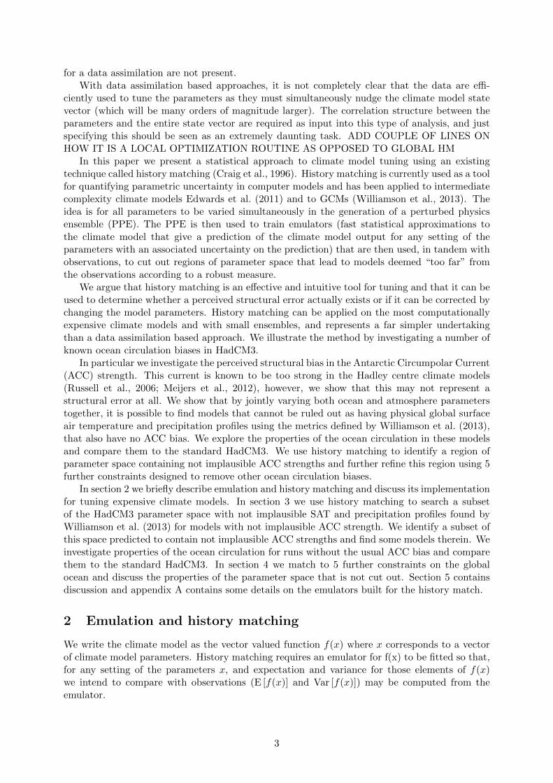
Figure 2 plots sea surface salinity (SSS) anomalies (left panels) and the Barotropic streamfunc-tion (BSF, right panels) for the standard HadCM3 (top panels) and an NROY ensemble memberwith realistic ACC and AMOC strength (one of the red points in figure 1) in the bottom panels.The chosen ensemble member was representative of the difference between the standard HadCM3and those NROY members with realistic AMOCs and ACCs. A number of supposed “structuralerrors” in HadCM3 can be identified on the upper panels and have been improved by the alterna-tive parameter choice. For example, the standard HadCM3 has a fresh bias in the subpolar gyreand in the Norwegian sea that is not present in the alternative model. This is at the expense of aslight freshening of the subtropical gyre. However, it is perhaps more important that the salinityprofile is correct in the AMOC sinking regions.
The subpolar gyre is too far east in the standard HadCM3 and the subtropical gyre is toodiffuse. The improved ACC model has a much stronger subtropical gyre at the western boundaryand a shifted subpolar gyre that extends into the labrador sea as it should.
The gyres are not the only places we see improvements to the ocean circulation. Figure 3shows a cross section of the AMOC stream function at 26oN for the standard HadCM3 (top),the improved ACC model (middle) and the 1/12 degree NEMO ocean model ORCA12 (bottom).In the standard model the return flow is too shallow at the western boundary and there arereturn flows at the mid-Atlantic ridge and on the eastern boundary. The improved ACC modelcompares more favourably with ORCA12 with the North Atlantic Deep Water appearing morephysical on the western boundary and no large return flows away from it. By simply finding aNROY model with a more physical ACC strength at the drake passage, we have found a modelwith an improved ocean circulation in the North Atlantic.
8
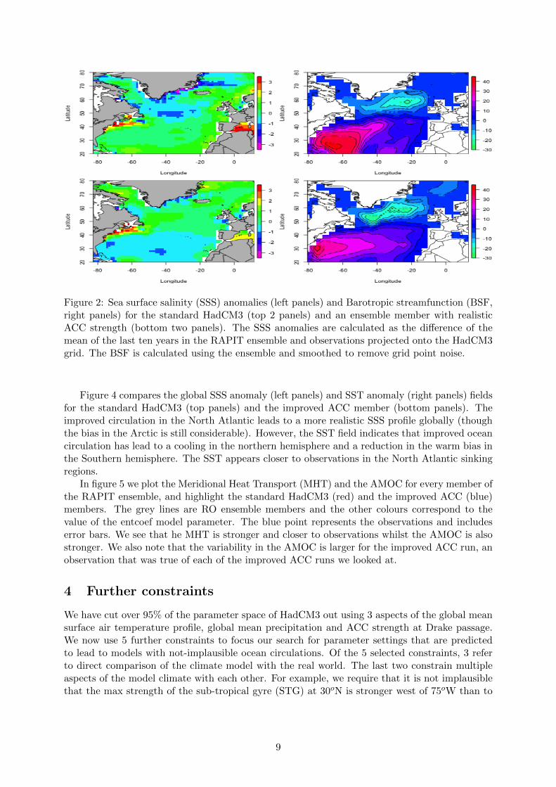
Figure 2: Sea surface salinity (SSS) anomalies (left panels) and Barotropic streamfunction (BSF,right panels) for the standard HadCM3 (top 2 panels) and an ensemble member with realisticACC strength (bottom two panels). The SSS anomalies are calculated as the difference of themean of the last ten years in the RAPIT ensemble and observations projected onto the HadCM3grid. The BSF is calculated using the ensemble and smoothed to remove grid point noise.
Figure 4 compares the global SSS anomaly (left panels) and SST anomaly (right panels) fieldsfor the standard HadCM3 (top panels) and the improved ACC member (bottom panels). Theimproved circulation in the North Atlantic leads to a more realistic SSS profile globally (thoughthe bias in the Arctic is still considerable). However, the SST field indicates that improved oceancirculation has lead to a cooling in the northern hemisphere and a reduction in the warm bias inthe Southern hemisphere. The SST appears closer to observations in the North Atlantic sinkingregions.
In figure 5 we plot the Meridional Heat Transport (MHT) and the AMOC for every member ofthe RAPIT ensemble, and highlight the standard HadCM3 (red) and the improved ACC (blue)members. The grey lines are RO ensemble members and the other colours correspond to thevalue of the entcoef model parameter. The blue point represents the observations and includeserror bars. We see that he MHT is stronger and closer to observations whilst the AMOC is alsostronger. We also note that the variability in the AMOC is larger for the improved ACC run, anobservation that was true of each of the improved ACC runs we looked at.
4 Further constraints
We have cut over 95% of the parameter space of HadCM3 out using 3 aspects of the global meansurface air temperature profile, global mean precipitation and ACC strength at Drake passage.We now use 5 further constraints to focus our search for parameter settings that are predictedto lead to models with not-implausible ocean circulations. Of the 5 selected constraints, 3 referto direct comparison of the climate model with the real world. The last two constrain multipleaspects of the model climate with each other. For example, we require that it is not implausiblethat the max strength of the sub-tropical gyre (STG) at 30oN is stronger west of 75oW than to
9

Figure 3: Cross section of the AMOC streamfunction at 26oN for the standard HadCM3 (top),an ensemble member with realistic ACC strength (middle), and ORCA 12 (bottom).
Figure 4: Left panels are global sea surface salinity anomalies and right panels and global seasurface temperature anomalies. The top panels are anomalies for the standard HadCM3 and thebottom panels are anomalies from an ensemble member with realistic ACC strength.
10

Figure 5: The Meridional Heat Transport (top panel) and AMOC time series for each memberof the RAPIT ensemble. Grey runs have been ruled out by history matching. NROY runs arecoloured by their value of entcoef. The highlighted red line in each image is the time series forthe standard HadCM3 and the highlighted blue line is the time series for our alternative withrealistic ACC transport. The curves on the left shows the unscaled density of the final year datafor the NROY part of the ensemble (blue) and the ruled out part of the ensemble (red).
the east. For constraints of the type nfi(x∗) > mfj(x
∗), the implausibility measure is
I(x) =mfj(x)− nfi(x)√
Var [mfj(x)− nfi(x)]
where
Var [mfj(x)− nfi(x)] = m2Var [fj(x)] + n2Var [fi(x)]− 2mnCov [fi(x), fj(x)] .
Large values of this type of implausibility, for some x0, indicate that even accounting for ouruncertainty about the values of fi(x0) and fj(x0), it is very unlikely that nfi(x) > mfj(x) sothat x0 can be ruled out as a possible setting of x∗.
Our first constraint is the SST anomaly in the sub-tropical gyre. By constraining with thismetric, we hope to find models with a more realistic global SST than those found in section 3.We define this metric to be the mean SST in a box from 70oW to 30oW and from 26oN to 36oN.The models with improved ocean circulation found in section 3 have anomalies of around 5oC inthis region. We specify a tolerance to error of half of that, so that we specify model discrepancywith a 3 standard deviation range of 2.5oC. Our discrepancy variance is therefore 0.69.
Though we do not have access to observation error for SST in this region, we note that theobservation error variance derived in Williamson et al. (2013) for global mean SAT was 0.0625,an order of magnitude lower than the discrepancy variance here. We also note that the region ofthe Atlantic we are assessing here is very well observed compared with global SAT, so that theobservation error variance is likely to be lower than for global mean SAT. We therefore ignoreobservation uncertainty for this constraint, taking the view that it is negligible relative to modeldiscrepancy variance.
11

Our next constraint is the maximum absolute sea surface salinity (SSS) in the sub-polar gyre(SPG), as it is believed that salinity in the sinking regions for the AMOC contributes towardsdeep convection and so may be a source of structural uncertainty in climate models. We takeSSS from a box from 50oW to 27.5oW and from 49oN to 57oN and had a tolerance to error forthe absolute maximum SSS in that box to be within 1 PSU of the observations. However, theabsolute maximum SSS turned out to be an unstable model output and was difficult to emulate.We therefore opted for the more stable mean of the largest 7 grid boxes in absolute value andrelaxed our tolerance to error by specifying a 3 standard deviation range of ±0.9PSU. As withSST we take the view that relative to this the observation error is negligible as this region of theAtlantic is well observed.
Our next two constraints demand that the location of the gyres is broadly physical. First,we constrain the STG to be closer to the western boundary by demanding that the maximumtransport at 30oN is west of 75oW. The second demands that the SPG is in a more physicallocation by ensuring that the mean of the gyre transport in the strongest 7 grid boxes in a boxbetween 52oW and 37oW and 50oN and 58oN is 1.5 times stronger than that in a box between35oW and 18oW and 52oN and 62oN.
Our final constraint was upon the SST around the coast of iceland. In the standard HadCM3and the improved ocean circulation versions we had seen, there is a large warm SST bias aroundiceland (see figure 4). We constrain using mean SST in a box from 27oW to 10oW and from 62oNto 70oN in order to attempt to remove this “structural error”. We again assume that observationuncertainty is dominated by our tolerance to model error whose 3 standard deviation range wetake to be double that for SST in the STG at 5oC.
Given our new constraints, our implausibility function now has 7 levels requiring 12 emulatorsfor different outputs of HadCM3. The first level, with 4 emulators, checks whether a point x is inour original NROY space (Williamson et al., 2013). The next 6 check that it is not implausiblethat HadCM3, run at x, passes each of our 6 constraints, with those constraints comparing gyrestrengths at different locations, each requiring the evaluation of 2 emulators. The emulators forthe original NROY space are described in Williamson et al. (2013) and the remaining emulatorsare described in appendix A.
4.1 Results
To save computing power we match to each of the constraints in turn so that, for any x, if anyimplausibility is found to be greater than 3, the parameter setting is deemed implausible and theother constraints need not be checked.
The standard way to explore NROY space is by rejection sampling, where an x ∈ X isgenerated uniformly and accepted if I(x) < 3 (see,forexample Vernon et al., 2010; Williamsonet al., 2013). Williamson and Vernon (2013) develop a genetic search algorithm that the callimplausibility driven evolutionary Monte Carlo (IDEMC) designed to efficiently explore NROYspace over multiple waves of constraint and to generate uniform samples from the space. Thisis useful for subspaces of parameter space that are extremely small. In some applications, forexample, these subspaces can be less than 1 millionth of the size of the original space. The sizeof this space is near the limit of the capabilities of rejection sampling.
We generated 10000 samples from NROY space in order to determine some of its properties.We found that 0.47% of parameter space could not be ruled out using all 10 of our constraints.After matching to the ACC strength in section 3 we had ruled out over 95% of the parameterspace of HadCM3. This remaining NROY space is further reduced by 82.5% by restricting tonot implausible SST in the subtropical gyre, with SSS in the sub-polar gyre removing a further29.8% of that space. Only a further 0.4% is removed by restricting the location of the STG, anda further 8.2% is removed by demanding a more realistic sub-polar gyre. The final constraint onthe SST around iceland removed 4.5% of the remaining parameter space.
The relatively poor constraint provided by the SSS and the location of the gyres is due to a
12

Figure 6: Marginal probability density plots 9 of the parameters.
lack of predictability in the chosen constraints. The HadCM3 output was difficult to emulate forthese constraints in that the underlying parameter-based signal was dominated by noise. Thoughwe were able to validate each emulator by ensuring that predictions for ensemble members thatwere reserved from the emulators were accurate with respect to the emulator uncertainty, thisuncertainty was sufficiently large that the predictions were not very informative. This lead toa large variance on the denominator of the implausibility calculation for these constraints and,hence, lower implausibilities with diminished space reducing capabilities.
This highlights the need for care when defining the chosen constraints. They must be chosenso that they are physically interesting or important, but must also be responsive to changes inthe parameters and not dominated by internal variability. It may also be the case that newensembles with all members within the subspace NROY by the ACC and SST constraints wouldincrease the density of points in that region sufficiently to improve our emulators and generatefurther space reduction.
These results indicate that there is a small region of parameter space where we cannot ruleout the possibility that not only will our constraints on the ocean circulation be met, but therewill also be a not implausible SST and SSS profile in the north Atlantic. The uniform samplesthat we have generated from this region can be used to explore its shape and to discover which,if any, parameters can be tuned in order to lead us to this not implausible region.
Figure 6 shows marginal density plots for 9 of the more interesting atmosphere and oceanparameters. The first panel, showing the convective cloud entrainment rate coefficient, entcoef,indicates that low values of entcoef are implausible but that there are more NROY models at theupper end of its range than in the range between 2-4 that is often determined to contain the bestmodels (Sexton et al., 2011; Rowlands et al., 2012). Isopycnal diffusivity in the ocean (ahi1 si) isalso very active, with values towards the top end of its range favoured. The cloud droplet to rainconversion rate, ct, and the relative humidity threshold for cloud formation, rhcrit, have similarprofiles as do the cloud droplet to rain threshold over land, cwland, and the boundary layer cloud
13

Figure 7: Probability density plots for 2D projections of the parameters generated by kerneldensity estimation. White regions indicate parameter settings with no points in NROY space,the colour scale from low to high density is cyan, blue, purple, red, yellow.
fraction at saturation, eacf. There is also a similarity in the marginal form for the ocean mixedlayer parameters lamda, the wind mixing energy scaling factor and delta si, the wind mixingenergy decay depth, with lamda in particular quite active.
Perhaps more revealing are the probability density plots for 2D projections of the parameters,shown in figure 7. Each panel shows the approximate probability density of the samples projectedonto the two labelled dimensions, with high density coloured yellow, low density in blue, andwhite regions empty. The image reveals important interactions between parameters for differentprocesses.
We note that the conclusion we gained from figure 6 where lows values of entcoef are notimplausible can be seen from the white region at the bottom of each plot in the top row. Thereare other regions of space that are completely cut out with more interesting shape. For exampleif both ct and ahi1 si are near the bottom of their ranges, the parameter setting is implausible.However, if only one of these parameters is at the bottom of its range, it is possible to tunethe other parameters in order to obtain not implausible models. This is one way to spot crucialinteractions between parameters. We see similarly that when ct is low, there are ruled out regionsof parameter space when rhcrit is low or eacf, the boundary layer cloud fraction at saturation ishigh or lamda is low.
There are strong interactions between the ocean parameters with, in particular, a large regionof space cut out when lamda or delta si are low and ahi1 si is low. We also note a greater densityof predicted good points if both lamda and delta si are increased.
Though each panel shows interaction between the two relevant parameters, indicating thatthe parameters must be jointly varied in order to locate the not implausible region, the mostinteresting panels are those that show strong interactions between atmosphere and ocean param-
14

eters. For example, though the not implausible region is generally denser for high values of theisopycnal diffusivity in the ocean, a greater density of models can be found if ct is also high,cwland is also low or entcoef is in the centre of its range. This result shows that, in order to tunea climate model accurately, both ocean and atmosphere parameters must be varied together sothat these interactions can be revealed.
5 Discussion
Tuning a climate model with a high dimensional parameter space and a long run time is adifficult task. Currently this task is undertaken without taking advantage of the latest statisticaltechnologies for managing uncertainty in complex models. These methods allow for targetedand comprehensive search of parameter space for models satisfying numerous criteria. We haveargued that many perceived structural errors or “known biases” in climate models may be downto an inefficient search of the existing model parameter space during model development.
We have presented history matching, a technique already used to quantify parametric uncer-tainty with climate models, as a method for climate model tuning based on sound principles ofstatistical design. The method seeks to tune all parameters simultaneously by using PPEs andemulators to rule out regions of parameter space that lead to models that do not satisfy observa-tional constraints imposed by the model developers. We describe how the procedure should beundertaken iteratively, with new constraints and new PPEs used to refine the search for modelswithout perceived structural biases. We also discuss how to use coarse resolution versions of anexpensive model so that history matching can be used to assist in tuning the expensive versionwithout the requirement for large ensembles or long runs.
We have illustrated the power of this technique in investigating perceived structural biases inthe HadCM3 ocean circulation. We found that the perceived structural bias in the ACC strengthcould be corrected by jointly varying both cloud and ocean model parameters and showed thatthese changes also improved important physical properties of the ocean circulation, withoutcompromising the surface air temperature profile.
We showed that the location of the sub-polar gyre was more realistic in the models we foundthan in the standard HadCM3 and that the sub-tropical gyre was far more concentrated near thewestern boundary than previously thought possible for this model. We showed that the profileof North Atlantic deep water flows, unphysical in the standard HadCM3, compares favourablywith the current physical understanding of these flows as represented by the 1/12o NEMO oceanmodel.
We showed that the global sea surface salinity profile was closer to observations, but thatthe models found in this first wave of history matching had a larger cold bias in the northernhemisphere SST, though the Southern ocean warm bias in the standard HadCM3 was improved.
We then illustrated the method of iterative history matching by imposing 5 further constraintson parameter space designed to look for models with improved ocean circulations without thecold bias in the northern hemisphere SST. We ruled out over 99% of the model parameter spaceas possibly containing models that satisfied our constraints and showed the joint structure of theremaining space using 1 and 2 dimensional projections of 10000 uniform random samples fromit. We found that jointly tuning the cloud parameters, particularly entcoef, ct and rhcrit, withisopycnal diffusivity in the ocean, ahi1 si, and the mixed layer parameter lamda, was importantfor finding these regions of parameter space.
Though we have no further access to ensembles of HadCM3 as part of this work, a subset ofthese 10000 samples would represent a good design of a new PPE designed to further constrainthe HadCM3 parameter space. History matching is most effective with multiple waves of PPEs, asthe the emulators improve in the region of parameter space potentially containing good climatesdue to a higher density of model runs there. The improved emulators have lower variances, whichserves to increase implausibilities and rule out more space.
15

Our work suggests that an overly strong ACC strength in HadCM3 is not a structural error,but a calibration error. However, it may be the case that more realistic ACC strengths are onlypossible at the expense of introducing new biases in processes deemed more important than theACC by model developers. However, the best way we know of to find out for sure is to use historymatching with all of the important constraints included. If this is done at the model developmentstage, structural errors in a process can be identified by an attempt to history match using thatprocess ruling out all of the parameter space. If the constraints are introduced iteratively, inorder of importance, the modellers can determine where the structural errors are and use thisinformation to focus their research into improving the model in order to reduce or remove theseerrors.
Given the cost of developing GCMs and their importance for decision making and globalpolicy strategy, it is important that every opportunity to improve the accuracy of these modelsis taken. History matching offers a robust and rigorous statistical methodology that is easy toimplement and can be used to help to efficiently tune the parameters of GCMs.
Acknowledgements
This research was funded by the NERC RAPID-RAPIT project (NE/G015368/1). We would liketo thank the CPDN team for their work on submitting our ensemble to CPDN users. We’d alsolike to thank the Institute of Advanced Study at Durham University for funding and hosting ourworkshop on ocean model discrepancy which formed the motivation for these investigations. Inaddition, we thank the oceanographers who participated in this workshop. We’d like to thankthe CPDN users around the world who contributed their spare computing resource as part of thegeneration of our ensemble.
ReferencesAcreman, D. M. and Jeffery, C. D. (2007), “The use of Argo for validation and tuning of mixed layer models,” Ocean. Model.,
19, 53–69.
Annan, J. D., Hargreaves, J. C., Edwards, N. R., Marsh, R. (2005), “Parameter estimation in an intermediate complexityearth system model using an ensemble Kalman filter”, Ocean Modelling, 8, 135–154.
Annan, J. D., Lunt, D. J., Hargreaves, J. C., Valdes, P. J. (2005), “Parameter estimation in an atmospheric GCM using theensemble Kalman filter”, Nonlinear Processes in Geophysics, 12, 363–371.
Annan, J. D., Hargreaves, J. C., Ohgaito, R., Abe-Ouchi, A., Emori, S. (2005) “Efficiently constraining climate sensitivitywith ensembles of paleoclimate simulations”, SOLA, 1, 181-184, doi:10.2151/sola.2005-047.
Challenor, P., McNeall, D., and Gattiker, J. (2009), “Assessing the probability of rare climate events,” in The handbook ofapplied Bayesian analysis, eds. O’Hagan, A. and West, M., Oxford University Press, chap. 10.
Collins, M., Brierley, C. M., MacVean, M., Booth, B. B. B. and Harris, G. R. (2007) “The Sensitivity of the Rate of TransientClimate Change to Ocean Physics Perturbations,” J. Clim., 20, 23315–2320.
Craig, P. S., Goldstein, M., Seheult, A. H., and Smith, J. A. (1996), “Bayes Linear Strategies for Matching HydrocarbonReservoir History,” in Bayesian Statistics 5, eds. Bernado, J. M., Berger, J. O., Dawid, A. P., and Smith, A. F. M., OxfordUniversity Press, pp. 69–95.
Craig, P. S., Goldstein, M., Rougier J. C., and Seheult, A. H. (2001), “Bayesian Forecasting for Complex Systems usingComputer Simulators,” J. Am. Stat. Assoc., 96, 717–729.
Cumming, J. A. and Goldstein, M. (2009), “Small sample designs for complex high-dimensional models based on fastapproximations,” Technometrics, 51, 377–388.
Cunningham, S. A., Alderson, S. G., King, B. A. (2003) “Transport and variability of the Antarctic Circumpolar Current inDrake Passage”, Journal of Geophysical Research, 108, No. C5, 8084, doi:10.1029/2001JC001147.
Daniel, C. (1973) “One at a time plans”, Journal of the American Statistical Association, 68, 353–360.
Draper, N. R., Smith, H. (1998), “Applied Regression Analysis,” 3rd Edition, John Wiley and Sons, New York.
Edwards, N. R., Cameron, D., Rougier, J. C. (2011), “Precalibrating an intermediate complexity climate model”, Clim.Dyn., 37, 1469–1482.
16

Fisher, R. (1926) “The arrangement of field experiments”, Journal of the Ministry of Agriculture of Great Britain, 33,503–513.
Friedman, M., Savage, L. J. (1947) “Planning experiments seeking maxima”, in Techniques of Statistical Analysis, edsEisnenhart, C., Hastay, M. W., Wallis, W. A. New York: McGraw-Hill.
Gent, P. R., Danabasoglu, G., Donner, L. J., Holland, M. M., Hunke, E. C., Jayne, S. R., Lawrence, D. M., Neale, R. B.,Rasch, P. J., Vertenstein, M., Worley, P. H., Yang, Z, Zhang, M. (2011), “The Community Climate System Model Version4”, Journal of Climate, 24, 4973–4991.
Goldstein, M and Rougier, J. C. (2009), “Reified Bayesian modelling and inference for physical systems”, J. Stat. Plan.Inference,139, 1221–1239.
Gordon, C., Cooper, C. Senior, C. A., Banks, H., Gregory, J. M., Johns, T. C., Mitchell, J. F. B., and Wood, R. A. (2000),“The simulation of SST, sea ice extents and ocean heat transports in a version of the Hadley Centre coupled model withoutflux adjustments,” Clim. Dyn., 16, 147–168.
Hargreaves, J. C., Annan, J. D., Edwards, N. R., Marsh, R. (2004), “A efficient climate forecasting method using anintermediate complexity Earch System Model and the ensemble Kalman filter”, Climate Dynamics, 23, 745–760.
Haylock, R. and O’Hagan, A. (1996), “On inference for outputs of computationally expensive algorithms with uncertaintyon the inputs,” in Bayesian Statistics 5, eds. Bernado, J. M., Berger, J. O., Dawid, A. P., and Smith, A. F. M., OxfordUniversity Press, pp. 629–637.
Kennedy, M. C. and O’Hagan, A. (2000), “Predicting the Output from a Complex Computer Code when Fast Approximationsare available,” Biometrika, 87.
Kennedy, M. C. and O’Hagan, A. (2001), “Bayesian Calibration of Computer Models,” J. R. Stat. Soc.. Ser. B, 63, 425–464.
Kraus, E. B. and Turner, J. (1967), “A one dimensional model of the seasonal thermocline II. The general theory and itsconsequences,” Tellus, 19, 98106
Martin, G. M., Milton, S. F., Senior, C. A., Brooks, M. E., Ineson, S., Reichler, T., Kim, J. (2010), “Analysis and reductionof systematic errors through a seamless approach to modelling weather and climate”, Journal of Climate, 23, 5933–5957.
Martin, G. M. and Coauthors (2011), “The HadGEM2 family of Met Office Unified Model Climate configurations”, Geosci.Model Dev., 4, 723–757.
Mauritsen, T., Stevens, B., Roeckner, E., Crueger, T., Esch, M., Giorgetta, M., Haak, H., Jungclaus, J., Klocke, D., Matei,D., Mikolajewicz, U., Notz, D., Pincus, R., Schmidt, H., Tomassini, L. (2012), “Tuning the climate of a global model”,Journal of advances in modeling Earth systems, 4, M00A01, doi:10.1029/2012MS000154.
Meehl, G. A., Covey, C., Delworth, T., Latif, M., McAvaney, B., Mitchell, J. F. B., Stouffer, R. J., and Taylor, K. E.(2007), “The WCRP CMIP3 multi-model dataset: a new era in climate change research,” Bull. Am. Meteorol. Soc., 88,1383–1394.
Meijers, A. J. S., Shuckburgh, E., Bruneau, N., Sallee, J. B., Bracegirdle, T. J., Wang, Z. (2012) “Representation of theAtarctic Circumpolar Current in the CMIP5 climate models and future changes under warming scenarios”. Journal ofGeophysical Research, 117, C12008, doi:10.1029/2012JC008412.
Murphy, J. M., Sexton, D. M. H., Jenkins, G. J., Booth, B. B. B., Brown, C. C., Clark, R. T., Collins, M., Harris, G. R.,Kendon, E. J., Betts, R. A., Brown, S. J., Humphrey, K. A., McCarthy, M. P., McDonald, R. E., Stephens, A., Wallace,C., Warren, R., Wilby, R., Wood, R. (2009), “UK Climate Projections Science Report: Climate change projections.” MetOffice Hadley Centre, Exeter, UK. http://ukclimateprojections.defra.gov.uk/images/stories/projections_pdfs/
UKCP09_Projections_V2.pdf
Pope, V.D. and M.L. Gallani and P.R. Rowntree and R.A. Stratton (2000), “The impact of new physical parameterizationsin the Hadley Centre climate model: HadAM3.”, Clim. Dyn., 16, 123–146.
Pukelsheim, F. (1994), “The three sigma rule”, Am. Stat., 48, 88–91.
Randall, D. A. and Coauthors, (2007), “Climate models and their evaluation”. Climate Change 2007: The Physical ScienceBasis, S. Solomon et al. Eds., Cambridge University Press, 589–662.
Rougier, J. C. (2007), “Probabilistic inference for future climate using an ensemble of climate model evaluations”, ClimaticChange, 81, 247–264.
Rougier, J. C. (2008), “Efficient emulators for multivariate deterministic functions,” Journal of Computational and GraphicalStatistics, 17, 827 – 843.
Rougier, J. C., Sexton, D. M. H., Murphy, J. M., and Stainforth, D. (2009), “Emulating the sensitivity of the HadSM3climate model using ensembles from different but related experiments,” J. Clim., 22, 3540–3557.
17
Rowlands, D. J., Frame, D. J., Ackerley, D., Aina, T., Booth, B. B. B., Christensen, C., Collins, M., Faull, N., Forest, C. E.,Grandey, B. S., Gryspeerdt, E., Highwood, E. J., Ingram, W., J., Knight, S., Lopez, A., Massey, N., McNamara, F.,Meinshausen, N., Piani, C., Rosier, S., M., Sanderson, B., J., Smith, L. A., Stone, D. A., Thurston, M., Yamazaki, K.,Yamazaki, Y., H., Allen, M. R. (2012), “Broad range of 2050 warming from an observationally constrained large climatemodel ensemble”, Nat. Geosci., published online, doi:10.1038/NGEO1430.
Russell, J. L., Stouffer, R. J., Dixon, K. W. (206) “Intercomparisons of the Southern ocean circulations in IPCC coupledmodel control simulations”, Journal of Climate, 19, 4560–4575.
Sacks, J., Welch, W. J., Mitchell, T. J., and Wynn, H. P. (1989), “Design and Analysis of Computer Experiments,” Stat.Sci., 4, 409–435.
Santner, T. J., Williams, B. J., and Notz, W. I. (2003), The design and analysis of computer experiments, Springer-VerlagNew York.
Severijns, C. A., Hazeleger, W. (2005), “Optimizing parameters in an atmospheric general circulation model”, Journal ofClimate, 18, 3527–3535.
Sexton, D. M. H., J. M. Murphy, and M. Collins (2011) “Multivariate probabilistic projections using imperfect climate modelspart 1: outline of methodology”, Clim. Dyn., doi:10.1007/s00382-011-1208-9.
Solomon, S., Qin, D., Manning, M., Chen, Z., Marquis, M., Averyt, K. B., Tignor, M., and Miller, H. L. (eds.) (2007),Contribution of Working Group I to the Fourth Assessment Report of the Intergovernmental Panel on Climate Change,2007, Cambridge University Press.
Vernon, I., Goldstein, M., and Bower, R. G. (2010), “Galaxy Formation: a Bayesian Uncertainty Analysis,” Bayesian Anal.5(4), 619–846, with Discussion.
Watanabe, M., Suzuki, T., O’Ishi, R., Komuro, Y., Watanabe, S., Emori, S., Takemura, T., Chikira, M., Ogura, T., Sekiguchi,M., Takata, K., Yamazaki, D., Yokohata, T., Nozawa, T., Hasumi, H., Tatebe, H., Kimoto, M. (2010), “Improved climatesimulation by MIROC5: Mean states, variability and climate sensitivity”, Journal of Climate, 23, 6312-6335.
Williamson, D. (2010), “Policy making using computer simulators for complex physical systems; Bayesian decision supportfor the development of adaptive strategies,” Ph.D. thesis, Durham University.
Williamson, D., Goldstein, M. and Blaker, A. (2012), “Fast Linked Analyses for Scenario based Hierarchies,” J. R. Stat. Soc.Ser. C, 61(5), 665–692.
Williamson, D., Goldstein, M., Allison, L., Blaker, A., Challenor, P. Jackson, L., Yamazaki, K., (2012b), “History matchingfor exploring and reducing climate model parameter space using observations and a large perturbed physics ensemble”,Climate Dynamics, To Appear.
Williamson, D., Blaker, A. T. (2013), “Evolving Bayesian emulators for structured chaotic time series, with application tolarge climate models”, SIAM J. Uncertainty Quantification, Accepted.
Williamson, D., Goldstein, M. (2013) “On the use of evolving computer models in Bayesian decision support”, Journal ofStatistical Planning and Inference, In Submission.
Williamson, D., Vernon, I. R. (2013) “Implausibility driven Evolutionary Monte Carlo for efficient generation of uniform andoptimal designs for multi-wave computer experiments”, Journal of the American Statistical Association, In Submission.
Yamazaki, K., Rowlands, D. J., Aina, T., Blaker, A., Bowery, A., Massey, N., Miller, J., Rye, C., Tett, S. F. B., Williamson,D., Yamazaki, Y. H., Allen, M. R. (2012), “Obtaining diverse behaviours in a climate model without the use of fluxadjustments”, Journal of Geophysical Research - Atmospheres, Accepted.
A Building emulators for history matching
What follows is a brief description of the methods we used to construct emulators for the con-straints described in this paper. As discussed in section 2 there are many ways to build emulatorsand the way that is chosen will depend on the size of the PPE available, the type of constraint wewish to emulate and the relationships between the data and the parameters that we find. In thisstudy we had access to large ensembles, and each of our constraints was a univariate quantity andso required less sophisticated modelling than a spatial field or time series might. Hence we fit theemulator mean functions, βg(x) in equation 1 using a stepwise regression procedure describedbelow.
The functions we consider adding to g(x) were linear, quadratic and cubic terms in each ofthe parameters with up to third order interactions between all parameters considered. Switch
18
parameters were treated as factors (variables with a small number of distinct possible “levels”)and interactions between factors and all continuous parameters were permitted.
Our fitting procedure begins with a “forward selection”, where we permit each allowed termto be added to g(x) in its lowest available form. For example, if the linear term for vf1 is notyet in g(x), vf1 is available for selection but vf12 is not. If vf1 is already in g(x) then all firstorder interactions with the other linear parameters in g(x) are included and then vf12 is availablefor selection. So, suppose g(x) is (1, entcoef), then the selection of vf1 implies that g(x) willbecome (1, entcoef, vf1, vf1*entcoef). If vf1 is selected, at the next iteration we may select anyof the other parameters but we may also include quadratic terms entcoef2 and vf12. We add theinteractions in this way, and do similar for third order interactions when quadratic terms havebeen included, so that the resulting emulator will be robust to changes of scale (see Draper andSmith, 1998, for discussion). The term that is added to g(x) at each iteration is the term of thoseavailable that reduces the residual sum of squares the most after fitting by ordinary least squares.
When it becomes clear that adding more terms is not improving the predictive power of theemulator (a judgement made by the analyst based on looking at the proportion of variabilityexplained by the emulator and at plots of the residuals from the fit) we begin a backwardselimination algorithm. This removes terms from g(x), strictly one at a time, with the leastcontribution to the sum of squares explained by the fit without compromising the quality of thefit. Lower order terms are not permitted to be removed from g(x) whilst higher order termsremain. We stop when removing the next term chosen by the algorithm leads to a poorerstatistical model. For more details on stepwise methods such as these see Draper and Smith(1998).
We allow ε(x) in equation 1 to be mean zero error with variance specified by the residualvariability from the fits and no correlation between ε(x) and ε(x′) for x 6= x′. Though thislack of correlation might not be appropriate if we had smaller ensembles or, perhaps, if we hadcompleted a number of waves of history matching and were focussing on a densely sampled subsetof parameter space, it is computationally efficient and a reasonable enough approximation to thedata here to be adopted for pragmatism.
Following the fitting of each emulator we validate its quality using 10% of the ensemble thatwas chosen randomly and reserved from the training data prior to the fit. This procedure involveschecking that the emulator accurately predicts each of the unseen ensemble members to withinthe accuracy specified by emulator uncertainty. If the emulators pass this diagnostic check, wethen use them in our history matching.
We give details of our emulator for the ACC strength in HadCM3 to illustrate the complexityof the mean function and the performance of the predictions. The terms selected in g(x) aredisplayed in table 1. Each header corresponds to the names of one of the parameters shortened inan obvious way. Numbers on the diagonal of the table refer to the order of the parameter includedin the emulator. For example, the number 2 implies that both quadratic and linear terms in thatparameter were included in g(x). Numbers on the upper triangle refer to the inclusion (1) or not(0) of interactions between the two relevant parameters in g(x). So, reading from the first row ofthe table, the term (ent ∗ ct) is included in g(x), but the term (ent ∗ rhct) is not. Variables inbold on the lower triangle indicate the inclusion of the given third order interaction. For example,the table indicates that the term (ah2∗cwl) is in g(x). In addition to the terms in the table, thefactor r layers and a linear term in parameter charnock are included, as is 1 so that an interceptis fitted.
Figure 8 shows a validation plot for the ACC emulator. For 65 PPE members, chosen ran-domly, that were reserved from the emulator at the fitting stage, the data are sorted by ACCstrength and plotted in red. We overlay the emulator predictions (black points) and the uncer-tainty on those predictions (error bars). The uncertainty represents approximately 2 standarddeviations for each prediction. We can see that the predictions are generally good with mostunseen PPE members laying within the uncertainty on the prediction. In fact, our uncertainty
19

Table 1: A table indicating which terms are in g(x) for our emulator of ACC in equation (1). Thecolumn and row names refer to the parameter names, shortened in an obvious way in order tosave space. The upper triangle labels which interaction pairs are present. The diagonal indicatesthe order of the highest order term in that variable. The lower triangle indicates which three wayinteractions are included.
ent ct rhct eac cwl vf ah ddif g0 min lam del dkap kap asy ddel
ent 2 1 0 1 1 1 1 0 0 0 0 1 0 1 1 1ct 1 1 0 0 1 0 0 1 1 0 0 0 0 0 0rhct 1 1 0 0 0 0 1 1 1 0 0 0 0 0eac ent 1 1 0 0 0 0 1 0 0 1 0 0 0cwl 1 0 1 0 0 0 0 0 0 0 0 0vf 1 0 0 0 0 0 0 0 1 0 0ah ent ah 2 0 0 1 0 0 1 0 0 0ddif 1 1 0 0 1 0 1 0 1g0 ah 1 1 0 0 0 0 0 0min 1 0 0 0 0 0 0lam 1 1 0 1 0 0del ent 1 0 1 0 0dkap 1 0 0 0kap vf 1 0 0asy 1 0ddel 1
specification may be too conservative, in that we have allowed for more uncertainty in the pre-dictions than is required. If this is the case, that would lead to less space ruled out by historymatching, not more, and it is our preference to remain conservative when ruling out regions ofparameter space.
20

Figure 8: Predicted ACC strength (black points) with error bars showing approximately 2 stan-dard deviations of the emulator uncertainty for each of the withheld PPE members (red points).
21