identifying and removing tilt noise from low-frequency...

952

Bulletin of the Seismological Society of America, 90, 4, pp. 952–963, August 2000

Identifying and Removing Tilt Noise from Low-Frequency (!0.1 Hz)

Seafloor Vertical Seismic Data

by Wayne C. Crawford and Spahr C. Webb

Abstract Low-frequency (!0.1 Hz) vertical-component seismic noise can be re-duced by 25 dB or more at seafloor seismic stations by subtracting the coherentsignals derived from (1) horizontal seismic observations associated with tilt noise,and (2) pressure measurements related to infragravity waves. The reduction in ef-fective noise levels is largest for the poorest stations: sites with soft sediments, highcurrents, shallow water, or a poorly leveled seismometer. The importance of preciseleveling is evident in our measurements: low-frequency background vertical seismicspectra measured on a seafloor seismometer leveled to within 1 ! 10"4 radians(0.006 degrees) are up to 20 dB quieter than on a nearby seismometer leveled towithin 3 ! 10"3 radians (0.2 degrees). The noise on the less precisely leveled sensorincreases with decreasing frequency and is correlated with ocean tides, indicatingthat it is caused by tilting due to seafloor currents flowing across the instrument. Atlow frequencies, this tilting generates a seismic signal by changing the gravitationalattraction on the geophones as they rotate with respect to the earth’s gravitationalfield. The effect is much stronger on the horizontal components than on the vertical,allowing significant reduction in vertical-component noise by subtracting the coher-ent horizontal component noise. This technique reduces the low-frequency verticalnoise on the less-precisely leveled seismometer to below the noise level on the pre-cisely leveled seismometer. The same technique can also be used to remove “back-ground” noise due to the seafloor pressure field (up to 25 dB noise reduction near0.02 Hz) and possibly due to other parameters such as temperature variations.

Introduction

Broadband seismology is moving into the oceans. Asthe recording capacities of ocean floor instrumentation im-prove and as broadband seismometers become smaller andlower power, seismologists have begun measuring broad-band (0.001–50 Hz) seismic signals at the seafloor to answerquestions that cannot be addressed with land-based seis-mometers. For example, researchers used a 320-km-wide ar-ray of ocean-bottom seismometers to study the structurebeneath the East Pacific Rise to 600-km depth usinglow-frequency teleseismic arrivals (the MELT experiment,Forsyth et al., 1998). In another recent experiment, Laske etal., (1998) measured Raleigh wave arrivals in the frequencyband between 0.014 and 0.07 Hz across an array of seafloordifferential pressure gauges to study lithosphere and upperaesthenosphere structure beneath the Hawaiian Swell. Per-manent broadband seafloor seismic stations are needed to fillin the gaps in global seismic networks (Montagner et al.,1998), and several researchers have studied noise and theeffects of seismometer emplacement for proposed perma-nent global seismic network stations (Montagner et al.,1994; Webb et al., 1994; Beauduin and Montagner, 1996;

Collins et al., 1998) and as part of local seismic networks(Romanowicz et al., 1998). A permanent broadband seismicstation was installed on an underwater cable between Hawaiiand California as part of the Hawaii-2 seafloor global seismicobservatory (Duennebier et al., 1998). Low-frequency seis-mic measurements can also be combined with pressure mea-surements to study the oceanic crustal melt distributionunder spreading centers using the compliance method(Crawford et al., 1999).

Unfortunately, the typical background seismic-noiselevel is much higher at the seafloor than on land, especiallyat frequencies below 1 Hz. Although the noise levels ob-served over one week at the French OFM pilot seismic station(in a borehole beneath the Atlantic Ocean) approach thenoise levels of good continental sites (Beauduin and Mon-tagner, 1996), most seafloor seismic measurements havemuch higher noise levels (Sutton and Barstow, 1990; Webbet al., 1994; Romanwicz et al., 1998). Some of the highestnoise has a tidal signature (Romanwicz et al., 1998), indi-cating that it is tied to currents. The noise may be diminishedby burying the sensor beneath the seafloor or placing it in a

Identifying and Removing Tilt Noise from Low-Frequency (!0.1 Hz) Seafloor Vertical Seismic Data 953

borehole (Montagner et al., 1994; Bradley et al., 1997; Col-lins et al., 1998), but this expensive option is probably onlyworthwhile for long-term or permanent stations.

In this article, we show how to reduce the vertical seis-mic noise level at frequencies below 0.1 Hz after the dataare acquired, by subtracting out the coherent signal fromother channels such as the horizontal geophones. On the or-der of 25 dB of the vertical seismic noise in the band from0.002 to 0.1 Hz can be caused by seafloor “compliance” orby tilt noise caused by seafloor currents. This noise can beremoved in the frequency or time domain, by generalizingthe technique described by Webb and Crawford (1999) toremove compliance noise.

Long-period vertical-component noise at the Pacificseafloor should in theory be dominated by the seafloor de-formation under the loading of very low-frequency oceanwaves (infragravity waves). In the absence of other noisesources, the pressure and vertical displacement are nearlyperfectly coherent at frequencies below about 0.05 Hz (thefrequency limit depends on the water depth), as the seafloordeforms under pressure loading (Crawford et al., 1998). Adifferential seafloor pressure gauge is an indispensable partof a broadband seismic station, both to remove the defor-mation signal from the seismic background spectrum and todetect other noise sources. The coherence between the ver-tical seismic and pressure measurements indicates the qual-ity of the low-frequency vertical-component data. Low co-herence in the frequency band 0.002–0.04 Hz suggests thatother noise sources, such as tilting due to ocean currents,dominate the “background” noise level.

The Experiment

We deployed two pressure-acceleration sensors in 900-m-deep water at 31"24#N, 118"42#W, at the outer edge ofthe California Continental borderlands. The sediments thereare about 1-km thick, and the seafloor is relatively flat. Theinstruments, deployed 1-km apart, collected data from 10September to 24 September 1998.

Both instruments carry a differential pressure gauge(Cox et al., 1984)) and a seismometer. In one instrument,the seismometer is a Lacoste-Romberg gravimeter (Lacoste,1967), in the other, a Streckeisen STS-2 three-componentbroadband seismometer. The gravimeter acts as a single-channel (vertical) long-period seismometer (Agnew et al.,1976). Both instruments sample twice per second, giving anupper (Nyquist) frequency limit of 1 Hz. The important dif-ferences between the two instruments are that (1) the STS-2 records horizontal and vertical motions, whereas the gra-vimeter measures only in the vertical, and (2) the gravimeteris much more precisely leveled than the STS-2.

Both the gravimeter and the STS-2 are leveled usingmotorized gimbals to center positions determined in the lab-oratory. We use a precise leveling system for the gravimeterbecause the measured gravity is very sensitive to cross-axistilt and because Lacoste-Romberg gravimeters become un-

stable if they tilt too far off of the long-axis center. On theseafloor, the gravimeter levels to within 5 ! 10"5 radiansof a laboratory-determined center value. We calculate thiscenter value by searching for the maximum apparent gravityas a function of the instrument cross level. The apparentgravity is gcos(h), where g is the local gravity (approxi-mately 9.8 m/sec2), and h is the cross-axis tilt from thevertical. The deviation in measured gravity equals g(1 "cos(h)) # 2gsin2(h/2). The centering precision depends onthe microseism noise that overlies the gravity signal. In thelaboratory, we can distinguish changes in apparent gravityas small as 8 ! 10"8 m/sec2, corresponding to a center valueuncertainty of approximately 1 ! 10"4 radians.

At the seafloor, the STS-2 levels to within 5 ! 10"3

radians of its center value. We estimated the STS-2 centervalue in the laboratory using a manufacturer-installed bubblelevel mounted on the seismometer base. The STS-2 hori-zontal and vertical channels are electronically derived frommeasurements of three geophones aligned in a cube-cornergeometry, allowing the sensor to correct for slightly off-levelemplacements. The sensor specifications suggest that theelectronics correction is accurate to within 1 ! 10"2 radi-ans. We will show that this inaccuracy can introduce signifi-cant vertical channel noise at the seafloor.

Seafloor Seismic Spectra

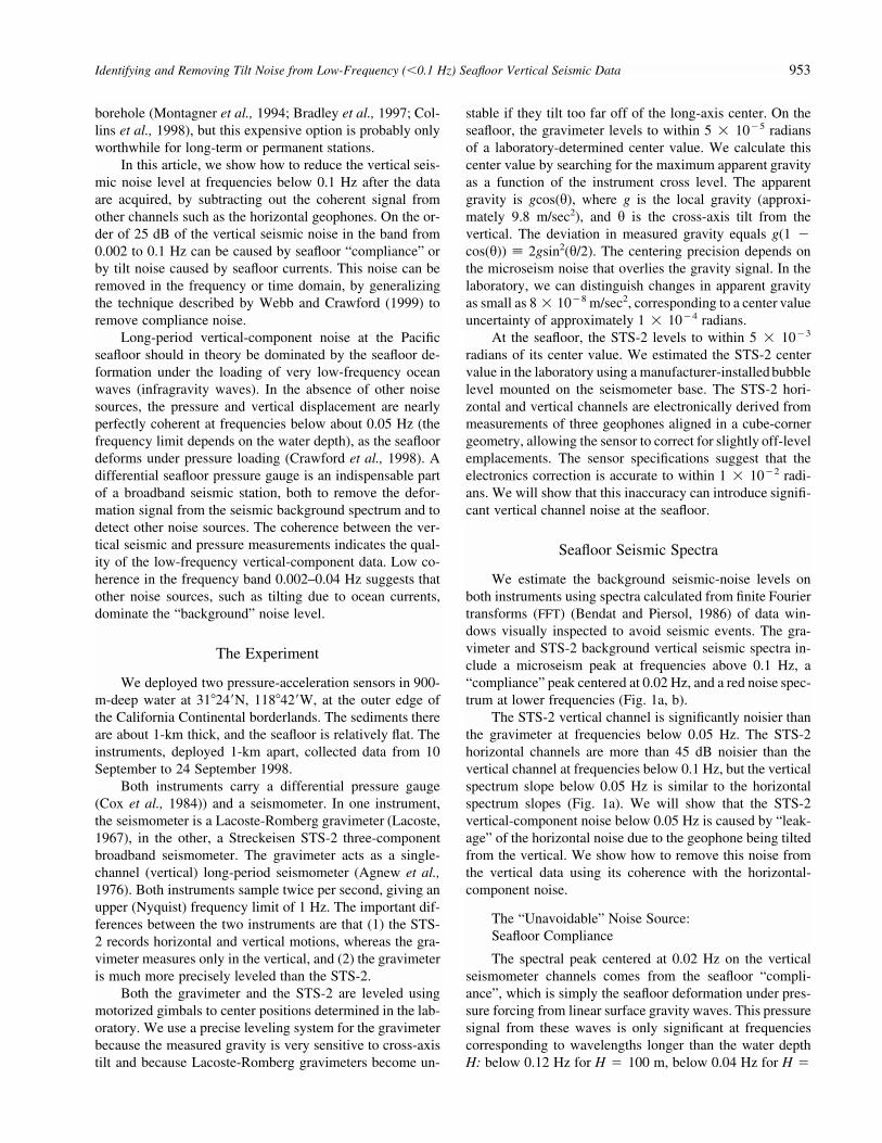
We estimate the background seismic-noise levels onboth instruments using spectra calculated from finite Fouriertransforms (FFT) (Bendat and Piersol, 1986) of data win-dows visually inspected to avoid seismic events. The gra-vimeter and STS-2 background vertical seismic spectra in-clude a microseism peak at frequencies above 0.1 Hz, a“compliance” peak centered at 0.02 Hz, and a red noise spec-trum at lower frequencies (Fig. 1a, b).

The STS-2 vertical channel is significantly noisier thanthe gravimeter at frequencies below 0.05 Hz. The STS-2horizontal channels are more than 45 dB noisier than thevertical channel at frequencies below 0.1 Hz, but the verticalspectrum slope below 0.05 Hz is similar to the horizontalspectrum slopes (Fig. 1a). We will show that the STS-2vertical-component noise below 0.05 Hz is caused by “leak-age” of the horizontal noise due to the geophone being tiltedfrom the vertical. We show how to remove this noise fromthe vertical data using its coherence with the horizontal-component noise.

The “Unavoidable” Noise Source:Seafloor Compliance

The spectral peak centered at 0.02 Hz on the verticalseismometer channels comes from the seafloor “compli-ance”, which is simply the seafloor deformation under pres-sure forcing from linear surface gravity waves. This pressuresignal from these waves is only significant at frequenciescorresponding to wavelengths longer than the water depthH: below 0.12 Hz for H $ 100 m, below 0.04 Hz for H $

954 W. C. Crawford and S. C. Webb

STS-2P

SD

(dB

rel

(m

/s2 )2 /H

z)

10-3

10-2

10-1

100

-160

-140

-120

-100

-80

Gravimeter

10-3

10-2

10-1

100

-160

-140

-120

-100

-80

10-3

10-2

10-1

100

0

0.2

0.4

0.6

0.8

1

Frequency (Hz)

P-Z

Coh

eren

ce

10-3

10-2

10-1

100

0

0.2

0.4

0.6

0.8

1

Frequency (Hz)

XYZ

a b

dc

Figure 1. “Background” seismic autospectral densities and pressure-vertical coher-ence from two seafloor seismometer/pressure gauge packages deployed 1-km apart onthe 900-m-deep seafloor. The shaded region in the spectra shows the bounds of seismicnoise observed on land stations (Peterson, 1993). One sensor contains a three-component, Streckeisen STS-2 broadband seismometer (left panels). The other sensorcontains a Lacoste-Romberg one-component (vertical) gravimeter (right panels). (a)STS-2 vertical and horizontal spectra. (b) Gravimeter vertical spectrum. (c) STS-2pressure-vertical coherence. (d) Gravimeter pressure-vertical coherence.

1000 m, and below 0.02 Hz for H $ 4000 m. The compli-ance signal jumps up rapidly below this frequency and thendecreases approximately proportionally to the frequency(Crawford, 1994). The compliance signal disappears behindnoise from other sources at a low-frequency limit that de-pends on this noise level.

In our data, the compliance peak rises above verticalbackground levels at frequencies between 0.004 and 0.05Hz, peaking at approximately "130 dB referenced to 1 (m/sec2)2/Hz, near 0.02 Hz. The compliance amplitude dependsmostly on the strength of the pressure signal (which is ap-proximately constant in the Pacific Ocean, but which maybe weaker and more variable in the Atlantic; Webb, 1998),and the shear modulus of the underlying basement. For agiven pressure signal, the deformation is approximately in-versely proportional to the basement shear modulus, so the

compliance signal is much stronger at a sedimented site thanat a hard-rock site (Crawford et al., 1998). The compliancesignal can be used to study the shear modulus or shear-velocity structure of the sediments and crust (Crawford etal., 1999), or it can be removed to allow easier detection ofother seismic signals (Webb and Crawford, 1999).

The compliance signal is not seen on the horizontalchannels. In theory, the horizontal compliance signal is 2–4times smaller than the vertical signal, but this is well belowthe measured horizontal background spectral levels. Not sur-prisingly, the horizontal-component data are incoherent withthe pressure data.

We can use seafloor compliance to evaluate the verticalseismic data quality in the frequency band between 0.001and 0.03 Hz. If there are no other significant noise sources,the pressure-acceleration coherence amplitude will be 1. A


decrease in the coherence indicates that there is another noisesource; coherence less than 0.5 indicates that the other noisesource is stronger than the compliance signal.

The pressure-gravimeter coherence has a larger ampli-tude and spans a larger frequency range than the STS-2pressure-vertical coherence, indicating that the STS-2 ver-tical senses more noncompliance noise than the gravimeter(Fig. 1c, d). The pressure-gravimeter coherence is above 0.9from 0.005–0.03 Hz, with a maximum coherence amplitude$0.999. On the STS-2, the pressure-vertical coherence isonly above 0.9 from 0.01–0.03 Hz, and the maximum co-herence amplitude is 0.98. The smaller amplitude and thehigher cut-off frequency of the STS-2 pressure-vertical co-herence indicates an additional low-frequency-noise sourcethat increases with decreasing frequency.

The “Extraneous” Noise Source: Seafloor Currents

Several lines of evidence indicate that the STS-2 verticalspectral levels below 0.01 Hz (and the horizontal spectralevels below 0.1 Hz) are dominated by tilting due to currents.First, the noise levels vary in sync with ocean tides. Second,the slope of the low-frequency noise is the same as that ob-served for seafloor currents. Third, the horizontal and ver-tical spectra have similar slopes and are coherent, with muchlarger noise levels on the horizontals. Finally, the noise isnot seen on the precisely leveled gravimeter.

The STS-2 background noise below 0.1 Hz fluctuateswith the tides. The noise is maximum when the first timederivative of the local ocean tides is maximum, and mini-mum when the first time derivative of the local ocean tidesis maximum (Fig. 2). The pressure-vertical coherence isweakest when the noise levels are highest. Seafloor currentsare primarily tidally driven although near-inertial motionscan contribute significantly (e.g., Thomson et al., 1990;Brink, 1995).

Current-induced tilt noise is caused by seafloor currentsflowing past the instrument and in eddies spun off the backof the instrument (Webb, 1988; Duennebier and Sutton,1995). We can model the effect of seismometer tilting onthe acceleration signal by assuming that the geophones atrest are rotated by an angle h from the vertical and are offsetfrom the instrument center of rotation (usually close to thecenter of mass) by a distance L and an angle h0 (Fig. 3)(Duennebier and Sutton, 1995). Current forcing rotates thegeophones around the center of mass by u $ u0 %!(x)cos(xt). This rotation creates acceleration signals on thegeophone by two processes: (1) a “displacement” term thatis the second derivative of the geophone position:

2% xta $ , x $ L sin(")x % L cos(")z (1)m t2%t

leading to

2 2a $ Lx e["cos u cos(xt) % e sin u cos(2xt) % O(e )]x 0 02 2a $ Lx e[sin u cos(xt) % e cos u cos(2xt) % O(e )]z 0 0

(2)

and (2) a “rotation” term that comes from the change in thegravitational acceleration on the geophones:

h $ g[sin(h % " ) " sinh]g t

e 2 2$ ge[cos h cos(xt) " sin h cos (xt) % O(e )]2

v $ g[cos(h % " ) " cos h]g t

e 2 2$ "ge[sin h cos(xt) % cos h cos (xt) % O(e )]2

(3)

where g is the gravitation acceleration (approximately 9.8m/sec2).

The total tilt-generated acceleration felt by the sensorsis

h $ a cos h % a sinh % ht x z g

2$ Lx e[cos h("cos u cos(xt) % e sin u cos(2xt))0 0

% sinh(sinu cos(xt) % e cos u cos(2xt))]0 0

e 2 2% ge[cos h cos(xt) " sin h cos (xt)] % O(e )2

(4)v $ a cos h % a sin h % vt z x g

2$ Lx e[cos h(sin u cos(xt) % e cos u cos(2xt))0 0

" sinh(cos u cos(xt) " e sin u cos(2xt))]0 0

e 2 2" ge[sinh cos(xt) % cosh cos (xt)] % O(e )2

In general, h, e K 1 and the geophone is not perfectly aboveor to the side of the center of mass (|"0 " np| $ e, n $ 0,1, 2, 3), simplifying equation 4 to:

2h $ e["Lx cos h cos(u ) cos(xt) % g cos h cos(xt)]02v $ e[Lx cos h sin(u ) cos(xt) " g(sin h cos(xt)0

e 2% cos(h) cos (xt))]2 (5)

The “displacement” (Lx2 . . . ) terms have positive am-plitude slopes and dominate at higher frequencies. The “ro-tation” terms (g . . . ) are independent of frequency and dom-inate at lower frequencies (Fig. 4). The rotational term isgenerally much larger on the horizontal channels than on thevertical, so low-frequency tilt noise is much larger on the hor-izontals than on the vertical. The vertical rotational term isapproximately (e/2 % sinh) times the horizontal rotational


-0.4-0.2 0 0.2

261

262

263

264

261

262

263

264

d(Ocean tide)/dT

Julia

n D

ay 1

998

Frequency (Hz)

Frequency (Hz)

P-Z coherence

Frequency (Hz)

X spectra (dB ref (m/s2)2/Hz)) Z spectra (dB ref (m/s2)2/Hz))

0.5 1-140 -140-160 -120-110 -80

10-2 10-110-3

10-2 10-110-3 10-2 10-110-3

originalcorrected

Figure 2. STS-2 horizontal and vertical spectra and pressure-vertical coherence ver-sus time and tides. Periods of high spectral noise are correlated with a high first deriv-ative of the ocean tide amplitude (calculated using the method of Agnew 1997). Toprow, uncorrected vertical channel; bottom row, vertical channel from which coherenthorizontal signals have been removed.

Figure 3. Schematic drawing of the geometryused to calculate the effect of tilt on the geophonesignal. The square represents the geophone, and C isthe center of rotation.

term. It is very small if the instrument is perfectly leveled, butit increases greatly if the geophone is even slightly off level.

The STS-2 low-frequency horizontals and vertical-noiselevels are well fit using equation 3 or 4 with a tilt spectrumSe(f ) $ 1.3 ! 10"2f "1.5 lradian2/Hz and a geophone tilth $ 3 ! 10"3 radians (0.2 degrees) (Fig. 5). The f "1.5

slope of the tilt spectrum is the same as the observed seafloorcurrent spectrum (Duennebier and Sutton, 1995; Webb,1998). The displacement of the geophone from the instru-ment center of mass, which plays a large role at higher fre-quencies, has no effect at frequencies below 0.1 Hz. A sim-ple rotation of the geophones to the vertical should reducethe vertical tilt noise level to near or below the continentallow-noise levels (Peterson, 1993).

The coherence between the three seismometer compo-nents (Fig. 6) help to illuminate the different background-noise sources. At frequencies above 0.1 Hz, the seismicchannels are all dominated by microseism energy, so theyare partly coherent with one another. At frequencies below0.1 Hz, the horizontals are dominated by tilt noise, and any


10-5

100

105

φ0≈0

φ0=π/4

φ0=π/2

θ=3x10-5 radiansθ=0 θ=3x10-2 radians

10-5

100

105

10-5

100

105

10-3 10-1

Frequency (Hz)

10110-3 10-1 10110-3 10-1 101

Sε=104 µrad2/Hz

Sε=1 µrad2/Hz

Sε=104 µrad2/Hz

Sε=1 µrad2/Hz

Sε=104 µrad2/Hz

Sε=1 µrad2/Hz

Sε=104 µrad2/Hz

Sε=1 µrad2/Hz

Sε=104 µrad2/Hz

Sε=1 µrad2/Hz

Sε=104 µrad2/Hz

Sε=1 µrad2/Hz

Sε=104 µrad2/Hz

Sε=1 µrad2/Hz

Sε=104 µrad2/Hz

Sε=1 µrad2/Hz

Sε=104 µrad2/Hz

Sε=1 µrad2/Hz

Figure 4. Tilt-acceleration transfer functions, assuming the geophone is 0.5 metersfrom the center of rotation. Thick lines show the overall transfer function, and thin linesshow the “rotation” (zero slope) and “displacement” (positive slope) components. Theonly important nonlinear term is the vertical acceleration due to rotation, which is signifi-cant if the geophones are perfectly leveled (h $ 0). The thinnest horizontal lines showthe transfer functions due to this nonlinear term, for constant tilt spectra Se(f) $ 1 and104 lradian2/Hz. Each row has the same angle between the geophone and the center ofrotation ("0) and each column has the same geophone tilt from the vertical (h).

horizontal-vertical coherence comes from tilt noise on thevertical. This coherence is high except over peaks in thevertical seismic energy (the “infragravity wave” peak at0.01–0.04 Hz and the small peak at 0.07 Hz, Fig. 1). Thereare no corresponding dips in the coherence between the twohorizontal channels, confirming that the horizontal seismicsignal below 0.1 Hz is dominated by tilt noise.

Removing Tilt Noise from the Vertical Channel

We remove the tilt-generated seismic background noiseby calculating the transfer function between the horizontaland vertical channels, and then subtracting the coherent hor-izontal energy from the vertical channel. For small geophonetilts this is equivalent to rotating the geophone back to the

vertical, except that it can reveal and remove other horizon-tal/vertical noise coupling not accounted for by our tiltmodel. This is the same technique we use to remove thepressure signal from the verticals (Webb and Crawford,1999), and can be generalized to remove vertical noise dueto other measured environmental variables such as tempera-ture. Our technique is inferior to rotation if nonlinear termsare important, but we prefer it because of its more generalapplicability and because nonlinear terms are generally in-significant compared to instrument noise levels and to thecontinental low-noise-level Model (Fig. 5). To subtract thetilt noise from the vertical component, we first estimatethe noise using the vertical-horizontal transfer functions. Wecan also estimate the vertical tilt noise in the time domainusing digital filters calculated from these transfer functions


φ0=0

10-3

10-2

10-1

100

101

-180

-160

-140

-120

-100

-80

φ0=π/2

10-3

10-2

10-1

100

10

-180

-160

-140

-120

-100

-80a bA

ccel

erat

ion

(dB

ref

(m

/s2 )2 /H

z)

Frequency (Hz) Frequency (Hz)

Figure 5. Modeled acceleration signals (Grey lines) versus seafloor STS-2 spectra(black lines). Dashed lines show the horizontal components, solid lines show the ver-tical component. Assumed tilt spectrum "t(f) $ 1.3 ! 10"2f"1.5 lradian2/Hz, L $0.5 m. The upper solid gray line is the modeled vertical acceleration for a geophonetilt of 3 ! 10"3 radians, and the lower solid gray line is the modeled vertical accel-eration for a perfectly leveled geophone. (a) Assuming the geophone is directly abovethe center of rotation ("0 $ 0); (b) assuming the geophone is to the side of the centerof rotation ("0 $ p/2).

Figure 6. Coherence between STS-2 seismometer channels. Upper plots show am-plitude; lower plots show phase. Z is the vertical channel, X and Y are the horizontalchannels. The dotted line in the amplitude plots marks the 95% significance level.

(see Appendix or Webb and Crawford, 1999, for details).Removing the noise in the time domain is useful for pickingseismic arrivals and modeling waveforms, whereas thefrequency-domain method is useful for spectral techniquessuch as normal mode analysis or seafloor compliance mea-surements.

To remove the low-frequency tilt and compliance noisefrom the vertical channel, we assume the horizontal channelsare completely controlled by tilt below 0.1 Hz and that theinfragravity signal is only on the pressure and vertical chan-nels (in other words, the horizontal components and pressuresignal are incoherent). Clearly some component of any ver-


tical seismic signal will be coherent with the horizontal chan-nels, however by a very large factor the horizontal channelsbelow 0.1 Hz on the seafloor are dominated by tilt. Becausethe horizontal-vertical transfer function is much smaller thanunity, the corrected vertical signal is unaffected by any realseismic signal on the horizontals. This method does not workabove 0.1 Hz because the seismometer channels are all dom-inated by the seismic “microseism” signal.

We first calculate frequency-domain transfer functionsbetween the different channels. To calculate the transferfunctions, we estimate the one-sided autospectral densityfunctions Gss and Grr from the Fourier transforms of win-dowed sections of data for variables s and r, (where s is the“source” channel (X, Y, or P) and r is the “response” channel(Z or Y)) and the one-sided cross-spectral density functionGrs to obtain the coherence function crs(f ):

nd2 N2G ( f ) $ |S ( f )| , j $ 0,1, . . . ,ss j ! i jn NDt 2i$1dnd2 N

G ( f ) $ R*( f )S ( f ), j $ 0,1, . . . ,rs j ! i j i jn NDt 2i$1d

G ( f )rsc ( f ) $ (6)rs j 1/2[G ( f )G ( f )]rr ssnd2 N2G ( f ) $ |R ( f )| , j $ 0,1, . . . ,rr j ! i jn NDt 2i$1d

where Si(f ) and Ri(f ) are fast Fourier transforms of data win-dow i for the source and response channels, nd is the numberof data windows, N is the length of each data window, andDt is the sampling interval (Bendat and Piersol, 1986). Eachwindow is tapered using a 4-pi prolate spheroidal functionto reduce broadband spectral leakage. The transfer functionArs(f ) is:

G ( f )rrA ( f ) $ c ( f ) (7)rs rs "G ( f )ss

In the frequency domain the noise seen in component ris linearly related to the s component through the transferfunction. The Fourier transform R# representing R correctedfor the noise in S is then:

R#( f ) $ R ( f ) " A*( f )S ( f ). (8)i i rs i

We calculate the various transfer functions between Z,X, Y, and P and correct the vertical component for noise seenin each of the other components in turn. We only want tosubtract the part of the source channel that is noise on thevertical so we set A(f ) $ 0 for frequencies above 0.1 Hzbefore applying equation 8.

Since the source channels may be coherent with oneanother, we must subtract out the coherent effect from allprevious “sources” before applying equation 8. Otherwise,the transfer function will include information about signals

already removed, adding noise to the vertical channel. Forexample, the two STS-2 horizontal channels are correlated,so we first apply equation 1 to remove the correlated part ofX from both the Z and Y components, forming Z# and Y#,then apply equation 1 to Z# and Y#. To subtract the coherentpressure signal, we calculate the transfer function betweenP and Z& (Z with the X and Y effects removed). This noisesuppression could also be done using multiple coherencetechniques, which perform an equivalent set of operations.

We also check to make sure the transfer functions don’tchange with time. If they do change (for example, if theinstrument tilt changes during an experiment), we wouldhave to calculate and apply different transfer functions be-fore and after the change.

An Example of Noise Removalin the Frequency Domain

To remove the vertical tilt-induced noise in the fre-quency domain, we first calculated the transfer functions be-tween the seismic channels (Fig. 7) in the relatively quiettime interval from 9 a.m. UMT 16 September to 1 a.m. UMT20 September 1998, skipping all time intervals containingnoise spikes or clipped horizontals. The transfer functionsbetween the vertical and horizontal components are roughlyconstant below 0.01 Hz where tilt noise dominates the ver-tical spectrum, and noisy and poorly resolved at higher fre-quencies where the compliance signal dominates the verticalspectrum. The near constant values at long period are con-sistent with a 0.003 radian vertical component tilt from thetrue vertical in x direction and a 0.001 radian tilt in the ydirection. The magnitudes of the horizontal-to-vertical trans-fer functions are small, so we are subtracting only a tinyfraction (less than 1 part in 300) of the horizontal channelsfrom the vertical channel. The effect of contamination ofvertical-component seismic waveforms by horizontal-com-ponent seismic motions caused by this processing is there-fore small.

The transfer function between horizontal components isa measure of the interaction of the two components due tothe flow noise and varies between 0.2 and 1.2. It is presum-ably a complicated function of the site response and the noisesource.

Using these transfer functions, we removed the coherenthorizontal data from the vertical as described previously. Toconfirm that all the coherent noise was removed, we recal-culated the coherence between the three seismic channels.The corrected Z channel is incoherent with the X and Ychannels for all frequencies below 0.1 Hz. The correctedvertical spectral noise levels (solid black line, Fig. 8a) areup to 20 dB lower than in the original spectrum. The coher-ence between pressure and the corrected STS-2 vertical isnow higher than and spans a larger frequency range than thepressure-gravimeter coherence (Fig. 8b). Even small im-provements in pressure-acceleration coherence are importantwhen using seafloor compliance to study crustal structure.

The corrected spectra significantly reduce the tidal ef-


Figure 7. Magnitude of transfer functions between the seismic channels (the phaseis the same as in Figure 6). The complex transfer function is used to subtract the effectof the horizontal channels on the vertical.

Z (

dB r

ef 1

(m

/s2 )2 /H

z))

-160

-150

-140

-130

-120

-110

-100STSSTS minus coh X & YSTS minus coh X, Y, & PL&R

10-3

10-2

10-1

100

0

0.2

0.4

0.6

0.8

1

Frequency (Hz)

P-Z

Coh

eren

ce

STSSTS minus coh X&YL&R

a

b

Figure 8. Vertical spectra and vertical-pressure coherence before and after removingcoherent noise from STS-2 horizontals. (a) Autospectral densities; (b) pressure-verticalcoherence.

fect on vertical seismic data (Fig. 2, bottom row). The cor-rected data are still slightly correlated with tides, but thecorrected vertical spectral noise levels are always lower thannoise levels from the same time in the original data. Thecorrected coherence also fluctuates slightly with the tides,

but the smallest corrected pressure-acceleration coherence islarger than the largest uncorrected acceleration-pressure co-herence.

Finally, to determine the effective noise floor for long-period seismic observations in this area, we removed the


Figure 9. STS-2 vertical seismic record of a magnitude 6.2 earthquake (D $ 44.2").All traces are bandpass-filtered between 0.001 and 0.05 Hz. (a) Original vertical trace;(b) vertical trace after subtracting coherent pressure signal; (c) vertical trace after sub-tracting coherent pressure and horizontal signals.

coherent pressure signal from the vertical spectrum (dash-dotted line, Fig. 8a). The new noise floor is 10–30 dB lowerthan in the original data at all frequencies below 0.04 Hz.

An Example of Noise Removal in the Time Domain

We applied the time-domain correction (see Appendix,and Webb and Crawford, 1999) to a section of data contain-ing the arrivals from a magnitude 6.2 earthquake 45.2" away(Aleutian Islands, 14 September 1998, Fig. 9). The earth-quake energy is mostly above 0.01 Hz, so the compliancecorrection is most noticeable, but the tilt correction is sig-nificant, particularly for waveform modeling. The horizontalcorrection will be more important at sites with low compli-ance (such as a hard-rock seafloor), larger currents, and/or amore tilted geophone.

Other Noise Sources

Below 0.003 Hz, the corrected STS-2 spectrum is lowerand its pressure-vertical coherence is higher than on the gra-vimeter. The higher gravimeter noise probably isn’t causedby currents. The gravimeter leveling uncertainty of approx-imately 1 ! 10"4 radians predicts a vertical noise level 76

dB below the horizontal noise level. The gravimeter spectrallevel is up to 67 dB below the STS-2 horizontal level ("154dB versus "79 dB at 0.004 Hz), and the gravimeter noiseslope below 0.004 Hz is much steeper than the STS-2 hor-izontal noise slope (Fig. 1). This very low frequency gravi-meter noise probably comes from temperature fluctuations,since Lacoste-Romberg gravimeters are much more tem-perature sensitive than STS-2 seismometers.

Discussion

We have shown how to remove tilt noise from low-frequency vertical-seismic data. This noise can be reducedby carefully leveling seismometers and by burying them insediments (Duennebier and Sutton, 1995) or perhaps byplacing in boreholes, although long-period seismic data fromseafloor boreholes up until now have been noisy, probablydue to convection currents (Webb, 1998). In addition, buriedinstallations are often impossible or economically unfeasi-ble. The technique we outline can transform a marginal dataset into a useful one, and is easily modified to account forother noise sources, even when their origin is not well un-derstood.


In the measurements shown here, the compliance noiseis generally larger than the tilt-induced noise, but this is notgenerally the case. We designed our seafloor sensors to mea-sure seafloor compliance (Crawford et al., 1998) and so welevel them more precisely than typical seafloor seismome-ters. Low-frequency vertical-seismic data from other sea-floor experiments such as MOISE (Romanowicz et al., 1998)and OSN-1 (Stephen et al., 1999) have red low-frequencybackground noise with the same slope as the horizontalnoise, indicating that they are dominated by tilt-generatednoise. Even the very quiet OFM site appears to be dominatedby tilt noise at low frequencies, probably because of a muchweaker compliance signal due to smaller infragravity wavesin the Atlantic Ocean (Webb, 1998).

We can not remove the tilt noise from the horizontalcomponent because it isn’t possible to construct a suffi-ciently accurate vertical reference (tilt sensor) that is alsoinsensitive to horizontal acceleration. Direct current mea-surements may be of little value since the horizontal tilt iscaused by the turbulent interaction of the current with thesensor case and surrounding seafloor. On sedimented sea-floors the tilt noise can be significantly reduced by buryingthe sensors a short distance below the seafloor. The theo-retical horizontal compliance signal is 2–4 times smallerthan the vertical compliance peak but measured horizontalspectra, even in buried and borehole sensors, are almost al-ways larger than vertical spectra (Montagner et al., 1994;Collins et al., 1998). The horizontal compliance peak in ourdata set would only be visible if the tilt spectrum is less than10"6 f "1.5 lradians2/Hz (dynamic tilts smaller than 0.03lradians near 0.01 Hz). Data from the recently emplacedHawaii-2 seafloor seismic observatory shows the first evi-dence for tilt levels this low (F. Duennebier, personal com-munication, 1999).

Seafloor noise levels can probably be reduced further.The vertical seismic-noise level after removing complianceand tilt effects is still well above the instrument noise floor,the predicted tilt noise, and the continental Low Noise LevelModel (Peterson, 1993). The vertical-component noise be-low 0.004 Hz is probably caused by temperature variations;adding sensitive temperature sensors to the instrumentshould allow us to further reduce this noise. Simultaneousrecordings of other environmental variables such as currentsand the magnetic field may allow us to identify and removefurther noise sources from seafloor seismic stations.

Acknowledgments

The seafloor measurements and data analysis were funded by U.S.Navy ARL Grant N00014-96-1-0297. We thank Jacques Lemire and TomDeaton for their help in developing and preparing the seafloor seismometer-pressure sensors. We also thank Charles Golden, Alexandra Sinclair, ChrisHalle, Tony Aja, Bill Gaines, and the crews of the R/P FLIP and the USNSNavajo for their help deploying and recovering the sensors.

References

Agnew, D., J. Berger, R. Buland, W. Farrell, and F. Gilbert (1976). Inter-national deployment of accelerometers: a network for very long pe-riod seismology, EOS Trans. Am. Geophys. Union 57, no. 4, 180–187.

Agnew, D. C. (1997). NLOADF: a program for computing ocean-tide load-ing, J. Geophys. Res. 102, no. 3, 5109–5110.

Beauduin, R., and J. P. Montagner (1996). Time evolution of broadbandseismic noise during the French pilot experiment of OFM/SISMOBS,Geophys. Res. Lett. 23, no. 21, 2995–2998, 1996.

Bendat, J. S., and A. G. Piersol (1986). Random Data: Analysis and Mea-surement Procedures, John Wiley and Sons, New York, 566 pp.

Bradley, C. R., R. A. Stephen, L. M. Dorman, and J. A. Orcutt (1997).Very low frequency (0.2–10.0 Hz) seismoacoustic noise below theseafloor, J. Geophys. Res. 102, no. 6, 11,703–11,718.

Brink, K. H. (1995). Tidal and lower frequency currents above FieberlingGuyot, J. Geophys. Res. 100, no. C6, 10,817–10,832.

Collins, J. A., F. L. Vernon, J. A. Orcutt, R. A. Stephen, J. R. Peal, J. A.Hildebrand, and P. N. Spiess (1998). Relative performance of theborehole, surficially-buried, and seafloor broadband seismographs onthe Ocean Seismic Network pilot experiment: frequency-domain re-sults, EOS Trans. Am. Geophys. Union 79, no. 45, 661.

Cox, C. S., T. Deaton, and S. C. Webb (1984). A deep sea differentialpressure gauge, J. Atmos. Oceanic Technol. 1, 237–246.

Crawford, W. C., S. C. Webb, and J. A. Hildebrand (1998). Estimatingshear velocities in the oceanic crust from compliance measurementsby two-dimensional finite difference modeling, J. Geophys. Res. 103,no. 5, 9895–9916.

Crawford, W. C., S. C. Webb, and J. A. Hildebrand (1999). Constraints onmelt in the lower crust and Moho at the East Pacific Rise, 9"48#N,using seafloor compliance measurements, J. Geophys. Res. 104, no.2, 2923–2939.

Duennebier, F. K., D. Harris, J. Jolly, K. Stiffel, J. Babinec, and J. Bosel(1998). The Hawaii-2 observatory seismic system, EOS Trans. Am.Geophys. Union 79, no. 45, 661.

Duennebier, F. K., and G. H. Sutton (1995). Fidelity of ocean bottom seis-mic observations, Mar. Geophys. Res. 17, 535–555.

Forsyth, D. W., D. S. Scheirer, S. C. Webb, L. M. Dorman, J. A. Orcut,A. J. Harding, D. K. Blackman, J. P. Morgan, R. S. Detrick, Y. Shen,C. J. Wolfe, J. P. Canales, D. R. Toomey, A. Sheehan, S. C. Solomon,and W. S. D. Wilcock (1998). Imaging the deep seismic structurebeneath a mid-ocean ridge; the MELT experiment, Science 280,1215–1218.

Lacoste, L. J. B. (1967). Measurement of gravity at sea and in the air, Rev.Geophys. 5, 477–526.

Laske, G., J. P. Morgan, and J. Orcutt (1998). Results from the HawaiianSWELL experiment, EOS Trans. Am. Geophys. Union 79, no. 45,662.

Montagner, J.-P., J.-F. Karczewski, B. Romanowicz, S. Bouaricha, P. Log-nonne, G. Roult, E. Stutzmann, J. L. Thirot, J. Brion, B. Dole, D.Fouassier, J.-C. Koenig, J. Savary, L. Floury, J. Dupond, A. Echar-dour, and H. Floc’h (1994). The French pilot experiment OFM-SIS-MOBS; first scientific results on noise level and event detection, Phys.Earth Plan. Int. 84, no. 1–4, 321–336.

Montagner, J.-P., P. Lognonne, R. Beauduin, G. Roult, J.-F. Karczewski,and E. Stutzmann (1998). Towards multiscalar and multiparameternetworks for the next century; the French efforts, Phys. Earth Plan.Int. 108, no. 2, 155–174.

Peterson, J. (1993). Observations and modeling of seismic backgroundnoise, U.S. Geol. Surv. Open-File Rept., Albuquerque.

Romanowicz, B., D. Stakes, J. P. Montagner, P. Tarits, R. Urhammer, M.Begnaud, E. Stutzmann, M. Pasyanos, J.-F. Karczewski, S. Etche-mendy, and D. Neuhauser (1998). MOISE: A pilot experiment to-wards long term sea-floor geophysical observatories, Earth PlanetsSpace 50, 927–937.


Stephen, R. A., J. A. Collins, J. A. Hildebrand, J. A. Orcutt, K. R. Peal,F. N. Spiess, and F. L. Vernon (1999). Seafloor seismic stations per-form well in study, EOS Trans. Am. Geophys. Union 80, no. 49, 592.

Sutton, G. H., and N. Barstow (1990). Ocean bottom ultra-low frequency(ULF) seismo-acoustic ambient noise: 0.002–0.4 Hz, J. Acoust. Soc.Am. 87, 2005–2012.

Thomson, R. E., S. E. Roth, and J. Dymond (1990). Near inertial motionsover a mid-ocean ridge: effects of topography and hydrothermalplumes, J. Geophys. Res. 95, no. C5, 7261–7278.

Webb, S. C., W. C. Crawford, and J. A. Hildebrand (1994). Long periodseismometer deployed at OSN-1, OSN Newsletter: Seismic Waves 3,no. 1, 4–6.

Webb, S. C. (1988). Long-period acoustic and seismic measurements andocean floor currents, IEEE J. Ocean Eng. 13, no. 4, 263–270.

Webb, S. C. (1998). Broadband seismology and noise under the ocean, Rev.Geophys. 36, no. 1, 105–142.

Webb, S. C., and W. C. Crawford (1999). Long period seafloor seismologyand deformation under ocean waves, Bull. Seis. Soc. Am. 89, no. 6,1535–1542.

Appendix

Removing Coherent Noise in the Time DomainTo remove the coherent noise from the vertical com-

ponent in the time domain, we first calculate the transferfunctions as described in the text. Here again, we assumethat P is incoherent with X and Y and that noise on the ver-tical component is because of tilt noise resolved on the x andy components and compliance noise resolved on the pressurecomponent. The x and y components are partly coherent, sowe first correct the z and y components for the effect of x(labeled z# and y#) and then correct z# for the effect of y#.

We calculate the inverse Fourier transforms (IFT) of thesevarious transform functions as shown below to derive digitalimpulse filters relating z to the x, y# and p components afterfiltering the transform functions to frequencies below 0.1 Hz.We subtract the noise in z due to these components by sub-tracting out the convolution of these digital filters with thedriving channels (Webb and Crawford, 1999). For example,to remove the current and compliance noise from the STS-2 vertical channel, calculate:

a (t) $ IFT(A# ( f ))zx zx

a (t) $ IFT(A# ( f ))yx yxa (t) $ IFT(A# ( f ))z#y# z#y#

a (t) $ IFT(A# ( f ))z&p z&p

The corrected time-domain vertical data z&(t) is then:

z&(t) $ z(t) " x(t)*a (t) " [y(t)zx

" x(t)*a (t)]*a (t) " p(t)*a (t)yx z#y# z &p

where x(t)*a(t) stands for the convolution of the data channelx(t) with the filter a(t). Note the quantity in brackets is y#(t),the y component corrected for x.

Scripps Institution of OceanographyUniversity of California, San DiegoLa Jolla, CA [email protected]

Manuscript received 19 August 1999.

identifying and removing tilt noise from low-frequency...

Documents