1

Identifying expertise and using it to extract the Wisdom of the Crowds

David V. Budescu & Eva Chen

Dept of Psychology, Fordham University, Bronx, NY 10458

Abstract

The "wisdom of the crowds" refers to the ability of statistical aggregates based on multiple

opinions to outperform individuals, including experts, in various prediction and estimation tasks.

For example, crowds have been shown to be effective at forecasting outcomes of future events.

We seek to improve the quality of such aggregates by eliminating poor performing individuals, if

we can identify them. We propose a new measure of contribution to assess the judges'

performance relative to the group and use positive contributors to build a weighting model for

aggregating forecasts. In Study 1, a dataset of 1,233 judges forecasting 104 binary current

events served to illustrate the superiority of our model over unweighted models and models

weighted by measures of absolute performance. We also demonstrate the validity of our model

by substituting the judges with fictitiously "random" judges. In Study 2, we used a dataset of 93

judges predicting winners of games for the 2007 NFL season and evaluated our model’s rate of

convergence with a benchmark of simulated experts. The model does an excellent job of

identifying the experts quite quickly. We show that the model derives its power by identifying

experts who have consistently outperformed the crowd.

1 Introduction

Nostradamus looked to the stars to foretell disasters, Gallup surveys the populace to model

future election outcomes, and sports commentators examines athletes’ past performances to

predict scores of future games (statistically and otherwise). Whether the discussion centers on

the art or the science of forecasting, decades of research have focused on the quality of

predictive judgments spanning various domains such as economics, finance, sports and popular

culture (e.g., Armstrong, 2001; Clemen & Winkler, 1999; Gaissmaier & Marewski, 2011;

Simmons, Nelson, Galak, & Frederick, 2011; Surowiecki, 2004). The simplest approach is to

solicit forecasts, but the literature suggests that individual judgments are riddled with biases,

such as being systematically too extreme or over-confident about reported probabilities, overly

anchored on an initial estimate, biased toward the most emotionally available information,

2

neglectful of the event’s base rate, etc. (Bettman, Luce & Payne, 1998; Dawes, 1979; Gilovich,

Griffin & Kahneman, 2002; Kahneman & Tversky, 2000; Simonson, 1989;). A natural remedy is to

seek experts in the relevant domain and hope that they would be less likely to succumb to such

biases. Unfortunately, expertise is ill defined and, not always easy to identify. Although in some

domains (e.g. short term precipitations) the experts are highly accurate (e.g, Wallsten &

Budescu, 1983), this is not the case in general (see, for example, Tetlock’s work in the political

domain, 2005).

An alternative approach that has received lots of attention recently is to improve

predictive judgment by mathematically combining multiple opinions or forecasts from groups of

individuals – knowledgeable experts or plain volunteers – rather than depend on a sole expert

(Hastie & Kameda, 2005; Larrick & Soll 2006; Soll & Larrick 2009) or a consensus derived from

interactions between the experts in the group (Sunstein, 2006). Surowiecki (2004) has labeled

this approach the “wisdom-of-crowds” (WOC). The claim is that some mathematical or statistical

aggregates (e.g., measures of central tendency) of the (presumably, independent) judgments of

a group of individuals will be more accurate compared to the typical or mean judge by exploiting

the benefit of error cancellation. Indeed, Larrick, Mannes, and Soll (2011) define the WOC effect

as the fact that the average of the judges beats the average judge. Davis-Stober, Budescu, Dana,

and Broomell (2012) propose a more general definition of the effect, namely that aggregate

linear combination of the crowd’s estimates should beat a randomly selected member of the

crowd.

The first demonstration of WOC is attributed to Francis Galton (1907) who, ironically,

hoped to show that “lay folks” are poor at making judgment even when guessing the weight of

an ox at a regional fair (Surowiecki, 2004). Instead, Sir Galton found that, although no individual

was able to accurately predict the precise weight, the crowd’s median estimate was surprisingly

precise, just one pound from the ox’s true weight. The performance of WOC depends on where

the truth is found in respect to the central tendency of judgments. Simple aggregates of the

crowd can be more accurate than the predictions of the best judges when the truth lies near the

average distribution of the forecasts. In instances when the truth is far from the central

tendency (e.g., at the tail or even away from the distribution), WOC produces predictions that

are equal or more accurate than the average judge, but not the best ones (Larrick et al. 2011).

3

The principles of WOC have been applied to many cases ranging from prediction

markets to informed policy making (Hastie & Kameda, 2005; Sunstein, 2006; Surowiecki, 2004;

Yaniv, 2004). Budescu (2006) suggests that aggregation of multiple sources of information is

appealing because it (a) maximizes the amount of information available for the decision,

estimation or prediction task; (b) reduces the potential impact of extreme or aberrant sources

that rely on faulty, unreliable and inaccurate information (Armstrong, 2001; Ariely, Au, Bender,

Budescu, Dietz, Gu, Wallsten & Zauberman, 2000; Clemen, 1989; Johnson, Budescu & Wallsten,

2001; Wallsten, Budescu & Diederich, 1997); and (c) increases the credibility and validity of the

aggregation process by making it more inclusive and ecologically representative. Interestingly,

the judges need not be “experts” and can be biased, as long as they have relevant information

that can be combined for a prediction (Hertwig, 2012; Hogarth, 1978; Koriat 2012; Makridakis &

Winkler, 1983; Wallsten & Diederich, 2001).

Critics of WOC have pointed to instances where the crowd’s wisdom has failed to deliver

accurate predictions because the aggregate estimate was largely distorted by systematic group

bias or by a large number of uninformed judges (Simmons et al., 2011). As an alternative to

simply averaging individual judgments by assigning equal weights to all, researchers have

proposed weighting models that favor better, wiser, judges in the crowd (Aspinall, 2010; Wang,

Kulkarni, Poor & Osherson, 2011). Such models are a compromise between the two extreme

views that favor quality (expertise) and those that rely on quantity (crowds). To benefit fully

from both the quality of the experts and the quantity of the crowd, the dilemma lies in assigning

appropriate weight or building a model to appropriately weigh the judgments (Budescu &

Rantilla, 2000).

We address this weighting problem and propose a novel measure of “contribution to

the crowd”, which assesses the individual predictive abilities based on the difference of the

accuracy of the crowd’s aggregate estimate with, and without, the judge’s estimate in a series of

previous forecasts in the domain of interest. This method explores the diversity of the crowd by

providing an easy to implement approach of identifying the best (and worst) individuals within

the crowd such that they can be over (and under) weighted. In the limit, the best subset of

judges can be identified and averaged while ignoring all the others.

4

We validate this individual contribution measure of performance, and test whether a

weighted model based on individual contributions to the crowd can be reliably better than

simply averaging estimates. Even when there is sufficient knowledge in the crowd to facilitate

prediction of future events, there is a strong element of chance involved in forecasting them, so

assessment of WOC needs to be performed over a substantial number of events and an

extended period of time. Imagine, for example, a stock market which, on average, gains in value

on 60% of the trading days (or a sports league where the home teams win 60% of the games)

and a forecaster who predicts its closing (results) on 10 independent days. There is a probability

of 0.367 (calculated by the Binomial with p = 0.6 and n = 10) that the market will not go up (or

that the home teams will not win) in a majority (6 or more) of the days. Thus, to measure

properly accuracy (of an individual or an aggregate) using cross-validation and dynamic

modeling one requires multiple, and preferably, longitudinal data. We consider two studies. The

first consists of events made over a few months regarding current events in five different

domains: business, economy, military, policy and politics. The second is based on a dataset from

Massey, Simmons and Armor (2011) on NFL football score predictions over games played during

a 17 week season.

2 Wisdom of the crowd

The premise behind WOC is that individual knowledge (signals) can be extracted, while biases or

misinformation (noise) can be eliminated by aggregating judgments (Makridakis & Winkler

1983). For the crowd to be wiser than the individuals, the distribution of estimated forecasts of

the individuals must “bracket” the actual value (Larrick & Soll, 2006). In essence, WOC requires

that judges in the group be knowledgeable, incentivized to express their beliefs, that the

responses be obtained independently from each other, and that there is a diversity of

knowledge to prevent any systematic bias of the group (see also Larrick, Mannes & Soll, 2011).

2.1 Diversity

One of the big selling points of WOC is that the aggregated estimate embodies a diversity of

opinions from the crowd. Indeed, successful implementations of WOC have gone out of their

way to foster diversity of opinions by: (1) selecting judges with different backgrounds, (2)

eliciting their inputs independently, and (3) forcefully injecting diverse thoughts to affect their

original estimates (Herzog & Hertwig, 2009).

5

Jain, Bearden and Filipowicz (2012) analyzed the accuracy of aggregated judgment as a

function of the diversity of personality in the crowd. The authors paired 350 participants. In each

pair, the two judges either had very similar or very different personalities (as measured by the

Big Five personality scores from McRae & John, 1992). Every judge was asked to forecast the

fate of a particular World Cup team and to guess the number of M&Ms candy in a jar. The

aggregated estimates from the diverse pairs were correct 42% of the time for the World Cup

teams compared to 32% for the similar pairs and 30% for individuals. The diverse pairs were also

the closest to the true number of M&Ms (23% off as compared to 26% off for the similar pairs

and 48% for the individuals). Although the underlying psychological principle at work is not

clear, these results highlight the benefit of selecting judges with different personalities and,

presumably, diverse opinions, to improve accuracy of predictions.

Diversity is derived not only from the group’s composition, but also from the method by

which information is shared in the group. If individuals are not given a chance to think

independently before responding, their judgments would be biased by responses from the

group (Larrick et al., 2011). In fact, the higher the correlation between the individual estimates,

the more judges are necessary to achieve the same level of accuracy (e.g., Broomell & Budescu,

2009; Clemen & Winkler, 1986; Hogarth, 1978). Lorenz, Rauhutb, Schweitzera, and Helbing

(2011) demonstrated that even mild social influence can undermine the effect of WOC in simple

estimation tasks. In their experiment 144 judges could reconsider their estimates to factual

questions after having received the mean, trend or full information of other judges’ estimates

but without interacting. The subjects’ estimates were compared for convergence of estimates

and improvements in accuracy over five consecutive rounds with a control (no information of

others’ estimates). The results showed that social influence triggers convergence of the

individual estimates and significantly reduces the diversity of the group without improving its

accuracy. However Miller and Steyvers (2012) showed that group aggregation performance on

more complex tasks, such as reconstructing the order of time-based and magnitude-based

series of items from memory, is better for judges who shared information with another judge

(after they have given their estimates) than for independent ones. Independent judgment

through the initial elicitation process (no social influence triggers) allowed for diversity of

judgment, and later information sharing can increased accuracy of estimates.

6

Taken to the extreme, WOC can be applied by treating the individual judge as a “pseudo

crowd”. Herzog and Hertwig (2009) changed the judges’ perceptions of the facts underlying the

event by asking the participants to assume that the first answer given was incorrect, to think of

reasons that the answer may be wrong, and provide a new answer. By forcefully injecting

diversity, the treatment elicited a greater variance of thought from the participants than simply

asking for repeated answers, and the results also produced the best aggregate estimated.

Diversity not only allows for greater variance, it serves to eliminate high degrees of correlation

among judges that can move the crowd to poor predictions.

2.2 Expertise

Of course, at least some of the judges must possess information , but in some cases the level of

information can be minimal. For example, Herzog and Hertwig (2011) report a study predicting

outcomes of three soccer and two tennis tournaments relying on the recognition heuristic.

Predictions based solely on the judges’ ability to recognize some of the players’ names (through

their exposure to different media) gave the group a diverse collective knowledge that was

sufficient to consistently perform above chance, and as accurately as predictions based on the

official rankings of the teams and players.

In most WOC forecasting applications the aggregation method gives equal weight to

judges without distinguishing any level of expertise. Indeed, most applications of WOC simply

average the judgments (Larrick et al., 2011)1. The outcome of such an approach may be sub-

optimal because it neglects external information (e.g., expertise) and, as such, reduces the

potential of benefiting from implicit wisdom to be found in the crowd. In a recent study,

Evgeniou, Fang, Hogarth, and Karelaia, (2012) found average deviations from consensus of

earnings per share increase as markets become more volatile especially for stock market

analysts of lower skills (measured by both past forecasting accuracy and education). The data

suggest that low performers tend to make bolder prediction – with the potential for greater

reward – driving the average prediction to more extreme positions. Lee Zhang and Shi (2011)

examined the bids of players on the popular game show “The Price Is Right.” The researchers

1 Jose, Grushka-Cockayne and Liechtendal (2012) make a case for robust measures based on trimmed or

windsorized means and Hora, Fransen, Hawkins, and Susel (2012) consider medians.

7

aggregated the bids to produce a price estimate that was superior to the individual estimates.

The aggregation models, especially those that took into account strategy and bidding history,

outperformed all the individuals, and the aggregation models that used external information

outperformed the simple mean. Thus, including the judges’ level of expertise could improve the

quality of the crowd’s forecasts.

WOC is about capturing the central tendency of the group that represents knowledge

beyond the grasp of any individual (Sniezek & Henry, 1989). Nevertheless, WOC is subject to

prediction failures that result from systematic biases and artificially high correlation among

judges2.

3 Aggregating probabilistic forecasts

We focus on aggregation of individuals who provide probabilities of future uncertain events.

Our goal is to combine the, possibly conflicting, probabilistic judgments made by different

individuals into one “best” judgment. French (2011) refers to this as “the expert problem.”

Typically, the judgments are probabilities or odds, but one could also combine qualitative

forecasts (see Wallsten, Budescu, & Zwick, 1993). The literature proposes two main paradigms

for combining individual judgments about uncertainties (Genest & Zidek, 1986): behavioral and

mathematical aggregations.

In behavioral aggregation the judges seek a consensus probability through an

interactive procedure, in which they revise their opinions after receiving feedback. The feedback

can vary from descriptive statistics of the group’s opinions to justifications on individual

probabilistic judgment. Examples of these techniques are the Delphi method, (see Rowe &

Wright, 2001 for a detailed description) and decision conferences (Phillips, 2007) among others.

Behavioral aggregation methods are not without criticism, the main one being that after several

rounds of interactions, the judges may still disagree, and some sort of non-behavioural

aggregation is needed. The second is that the benefits derived from the various methods are

2 Broomell and Budescu (2009) developed a quantitative model of the inter-judge correlations that

identifies the stand – alone contributions of several environmental and individual variables on the inter-

judge agreement.

8

highly dependent on the composition of the groups and the structure of the within group

interaction. Any change to the structure can compromise the interaction process, and thus

reduce the quality of the solution. The third criticism is that identifying real experts and

assembling a panel of experts can be costly without necessarily providing more accurate

forecasts (French, 2011).

The second paradigm is based on mathematical aggregation of the reported individual

probabilities. Two main approaches have been developed: Bayesian aggregation and opinion

pools (weighting models) (see Budescu & Yu, 2006). The Bayesian approaches treat the

individuals’ judgments as data and seek to develop appropriate likelihood functions that allow

the aggregation of probabilities by the Bayes formula applied to a prior probability judgment

(Clemen & Winkler, 1990). The key difficulty in this approach is the development of prior and

likelihood probability models. It is especially difficult to specify the covariance structure among

the data (experts). We focus on pooling because the approach is much simpler to implement

without making assumptions about priors, correlation of errors between experts, and likelihood

functions.

Opinion pools of the individuals’ probability judgments are the most frequently applied

weighting schemes in practice: from predictions of volcanic eruptions to risk assessments in the

nuclear power industry (Aspinall, 2010; Cooke & Goossens, 2004). Although there are more

general formulas (French, 1985; Genest & Zidek, 1986). the most common aggregation rules are

the weighted arithmetic (linear) and the weighted geometric pools (means):

and

where is the individual i’s reported probability for an event of interest (x) and the linear

opinion pool is the results from combining k individuals based on assignment of non-

negative weights (w), such that Σ = 1. In general, ≤ and, as a consequence, it

reduces the influence of the extremely high values. Variations of these themes involve averaging

9

the log-odds, log (pi/(1-pi)), and back transforming the mean log odds to the probability scale

(Bordley, 2011).

The weights in an opinion pool often represent the individuals’ relative expertise, but

the concept of “relative expertise” is ill defined and subject to many interpretations (French,

2011). One possibility is to assign weights based on individuating features of the judges. These

could be objective (e.g., historical track record, education level, seniority and professional

status), subjective (e.g., ratings of expertise provided by the judges themselves or others, such

as peers or supervisors) or a combination of the two. Another approach is to define the weights

empirically based on the experts’ performance on a set of uncertain “test” events, the

resolution of which are unknown to the experts, but known to the “aggregator” (person or

software) that assigns the weights in the opinion pool for the events of interest (Bedford &

Cooke, 2001; Cooke, 1991).

Clemen (2008) and Lin and Cheng (2009) have compared the performance of Cooke’s

empirical linear opinion pool method with equal weighting linear pools (“plain WOC”) and with

the best expert’s judgement. The weighted method generally outperformed both the equal

weights method and the best expert. Note, however, that the weights vary as a function of the

scoring rule used in the elicitation process and different scoring rules lead to different weights.

Wang et al. (2011) proposed that scores be accompanied by a cost (such as an incoherence

penalty based in part on violation of probability axioms and logic principles) to adequately weigh

individuals, especially in longitudinal and conditional probabilistic studies.

A critique of the empirical weighting linear pools is that they over-weight a few

individuals (i.e., true experts), which can lead to extreme predictions (Soll & Larrick, 2009). This

may be advantageous when there is a high correlation between the test events and the actual

events of interest. As the two sets of events diverge and the correlation between performances

of the two is reduced, an equal weighted average may be is preferable because equal weighting

values diversity of opinions, and downplays the “experts”. In this paper, we develop and employ

a new empirically weighted linear opinion pool (with a cost parameter). Unlike Cooke’s

approach, we do not use an independent stand-alone set of pre-test events to identify relative

expertise. Instead, the weights emerge in the process of forecasting and they are based on the

judges’ performance relative to others (i.e., contribution to the crowd). We also develop a

10

dynamic version of the model that adapts to changes in the contribution measure as new events

are being resolved and included in the model.

4 Contribution weighted model

We define an individual’s contribution to the crowd to be a measure of the individual expertise,

relative to the crowd. More specifically, it measures the change in the crowd’s aggregated

performance, with and without the target individual. Once such individual contributions are

calculated, a contribution weighted model (CWM) is devised to be applied in future predictions

by the same crowd of judges. To quantify the effects of WOC we need an appropriate measure

of quality of the aggregate (and the individuals). In the context of probability judgment this

score is, typically, a proper scoring rule (e.g. Bickel, 2007). We use the Brier score (Brier, 1950),

but the proposed approach and procedure can be applied to all other (proper or improper)

scoring schemes. To determine the contributions of each judge:

(1) The performance of the crowd of all N judges is aggregated across all the events,

based on the Brier score (Score):

where T is the number of forecasting instances (events), is the mean probability of the

crowd for event t (where t = 1...T) that takes a value between 0 and 1, and is the binary

indicator of the actual outcome for each event (0=occur or 1=not occur). In our case we use

constants a = 100 and b = -50, which yields Scores ranging from 0 to 100, where 0 indicates the

worst possible performance (assigning a probability of 1 to all events with = 0 and a

probability of 1 to all cases with = 0), 100 indicates perfect performance (assigning a mean

probability of 1 to all events with = 1 and a probability of 0 to all cases with = 0), and, 75 is

the expected score by “chance” (assigning a probability of 0.5 to all events).

(2) Each of the N judges is excluded (separately) from the crowd and the crowd’s Score

is recalculated based on the remaining (N-1) judges, to obtain N “partial” Scores (one for each

judge).

11

(3) The contribution of each judge is calculated by taking the difference between the

crowd’s original Score, and the “partial” Score without the target judge. Each judge’s

contribution can be expressed as the following:

where T is the number of events, is the mean transformed Brier score of the crowd (all N

forecasters) of each event, and is the corresponding mean Score, of that

event, of (N-1) forecasters, excluding the very judge (F) for whom the contribution is being

computed.

A judge’s contribution can be positive (indicating that his / her forecasts improve, on

average, the crowd’s Score) or negative (suggesting that his / her forecasts reduce the average

Score of the crowd), with an occasional 0 for judges whose presence or absence does not affect

the crowd’s mean performance. Clearly, we focus on, and value, positive contributions since the

higher is the contribution of a judge then the more he/she adds to the accuracy of the crowd.

This view of contribution is inspired by statistical literature on measures of influence

(e.g., Kutner, Nachtsheim, Neter, & Li, 2005), that seek to establish if, and by how much, various

parameters and predictions of complex statistical models are affected by specific observations,

by eliminating them (one at a time) from the sample. By analogy, we measure the influence of

each member of the crowd on the group’s performance in the relevant metric (in this case the

Score). We hypothesize that this measure would outperform weights based on the judges past

performance (“track record”). The key intuition behind this prediction is that, on average, and in

most cases the predictions of the various judges will be highly correlated (see Broomell &

Budescu, 2009 for a list of examples). Thus, there will be many cases where almost everyone in

the crowd will have very good Scores and, conversely, cases where practically all the members

of the crowd will perform poorly. Straight measures of absolute performance are not likely to be

very discriminating in such cases. Our contribution measure recognizes good performance in a

relative sense. Judges get high contribution scores if they do well in cases where the majority of

the crowds performs poorly, i.e., when they do not follow the crowd when it is wrong.

One does not necessarily have to perform exceptionally well, to stand out. Imagine an

event that is true (i.e., ot=1) and a crowd of (n-1) judges whose mean judged probability is p, so

12

their Brier score is (p-1)2. Now we consider a new judge, so the crowd’s size has increased to n.

The target judge’s prediction is closer to the truth, say p* = (p+Δ) where 0 ≤ Δ ≤ (1-p). The mean

probability of the new crowd is (p +Δ/n) and their Brier score is [(p-1) + Δ/n]2 . The difference

between the two Brier scores is [(Δ/n)2 – (2Δ(1-p)/n]. It is easy to show that this difference is

always negative (because Δ ≤ (1-p)). In other words, the Brier score with the new judge is closer

to the ideal 0. The magnitude of the improvement increases as a function of Δ and decreases as

the crowd size, n, grows. For example, assume (n-1) = 9 judges estimate the probability to be 0.2

with a Brier score of (1 - 0.2)2 = 0.64. The target judge’s estimate is 0.7 (Δ = 0.5) which is closer

to 1, but far from stellar. The new mean probability is 0.25 which yields a considerably better

Brier score of (1 - 0.25)2 = 0.5625. Under our scoring rule, this judges’ contribution would be

positive.

Our weighted aggregated model, CWM, employs only judges with positive contributions

in forecasting new events. These contributions are normalized to build weights, such that the

aggregated prediction of the crowd is the weighted mean of the positive contributors’

probabilities.

5 Study 1: Forecasting current events

To validate the weighting procedure and verify that it can identify quality judges in the crowd,

we analyzed data gathered from the ACES forecasting website (http://forecastingace.com).

Launched in July 2010, the website elicits probability forecasts from volunteer judges on current

events. The judges sign-up to become forecasters, and can choose to answer, at any time, any

subset of events from various domains including: business, economy, entertainment, health,

law, military, policy, politics, science and technology, social events, and sports. Although there

are a variety of event formats, we focus here only on binary ones that refer to occurrence of

specific target events. Each event describes a precise outcome that may, or may not occu,r by a

specific deadline (closing date) to allow an unambiguous determination of its ground truth at

the deadline. On average, 15 to 20 events are posted at various times every month with various

closing dates (some as short as 3 days and some as long as 6 months) as a function of the nature

of the event. There are no restrictions on the number of events a judge can answer, and every

week a newsletter is sent to all forecasters to announce new events being posted and

encourage participation.

13

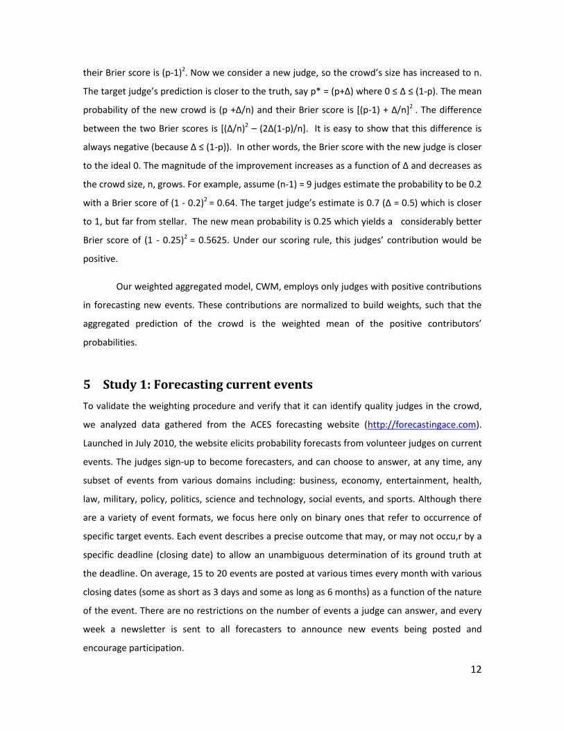
Figure 1 shows a screenshot of an event. Upon viewing the event, the judge first makes

a prediction on whether or not the event will occur, and then enters his / her subjective

probability of the event’s occurrence by moving the slider. The webpage enforces binary

additivity (i.e. forces the probability of the event occurring P(A) and the probability of the event

not occurring P(~A) to sum to 1). Judges have the option of listing rationales to justify their

forecast, but less than 10% of them provide rationales. The predictions and probabilities can be

revised any time before the closing date, but most judges (90%) do not revise their initial

judgments. The current data analysis was conducted only on the last reported probability for

every judge for any given event.

Figure 1 Screenshot of probability elicitation

The judges are scored based on their participation (number of forecasts performed) and

accuracy of prediction. The individual scores serve as an intrinsic motivator for participation and

they are the only explicit incentive provided by the website. In addition to providing forecasts,

judges were encouraged to complete a background questionnaire pertaining to their expertise

in the various domains. The questionnaire covers their self-assessed knowledge of the domains,

the hours they spend reading the news, education level, and years of experience in forecasting.

5.1 Data collection

1,233 judges provided probabilistic forecasts for 104 events between the launch of the site and

January 2012. The judges answered an average number of 10 events (i.e., on average judges

responded to 10% of the events posted) and the average number of respondents per event is

127. Only judges who had answered 10 or more events (n=420) were included in our analysis.

Some descriptive statistics are presented in Table 1. These judges responded to a mean number

14

of 23 events, reported a mean general knowledge on current issues around 5 (1 is no

knowledge, and 7 is extremely knowledgeable) and reported spending on average 23 minutes a

day reading the news. The level of education ranges from high school (4%) to Ph.D. (10%) and

most of them (64%) have at least a Bachelor’s degree. Only 37% of the judges have experience

in forecasting with an average of 5 years. Since judges could choose to make forecasts at various

times we derived a measure of timing3, that ranges from 0 (when an event is answered on the

day it is posted, or on the day a judge joins the site) and 1 (when an event is answered on the

date an event is scheduled to close, or on the date the outcome has occurred4). The mean

timing is 0.19 indicating that most events are answered close to the time they are posted. The

correlations between these variables and individual contributions can be found in the Appendix.

Table 1 Descriptive statistics of contributors (N=420):

Mean Min Q1 Median Q3 Max SD

Number of event answered 22.7 10 13 17 27 97 15.1

General knowledge (from 1 to 7) 5.01 2 4 5 6 7 0.83

Reading news (in hours) 0.39 0 0.25 0.33 0.50 1 0.26

Education (from 1 to 5) 3.17 1 2 3 4 5 1.07

Forecasting Experience (years) 5.20 0 0 0 6 50 0.91

Timing or response (relative to event duration)

0.19 0 0.10 0.17 0.25 1 0.14

5.2 Comparison of aggregation models

We hypothesized that CWM will provide more accurate forecasts by its method of

overweighting positive contributors and underweighting, or even dismissing, negative

contributors. The performance of CWM was compared against seven competing models listed in

Table 2.

Table 2 Alternaive aggregation models considered

3 Timing is the difference between the closing date of the item and the user submit date of the

reported probability, divided by the duration of the item, i.e., close date minus the open date , or

the period the user started participating, i.e., close date minus the first time the user submitted a

forecast , depending on whichever is the shortest period:

4 Some items are resolved at a predetermined fixed date (e.g. item about the mortgage rate in Figure 1),

but others can occur at any point in time prior to a given date (e.g. The DOWJ will drop below 12,000 at

anytime before the end of 2012),

15

Model Description Justification

ULinOp Equally weighted Score for all 1233 judges (the

crowd).

Test CWM against unweighted

Score of entire dataset.

UWM Equally weighted Score for the subset of 420

forecasters, who answered 10 or more events.

Test CWM against unweighted

Score of the same subset.

Contribution Equally weighted Score of all positive contributors

from the subset of 420 forecasters, who answered

10 or more events.

Compare the advantage of

weighting contributors.

BWM Weights are calculated with Score for all of the

420 judges. The weights depend only on the

judge’s past performace (Score).

Compare CWM with weighted

model based on absolute past

performance.

xBWM Same as BWM, but using a percentage of positive

contributors similar to CWM.

Compare CWM with weighted

model based on absolute past

performance with the same

number of positive contributors.

UnifCWM Instead of using the probabilities reported by the

judges to compute contribution as in CWM, the

probabilities are drawn from a uniform

distribution (0,1).

Assess the robustness of CWM

using uniform random distribution.

BetaCWM Instead of using the probabilities reported by the

judges to compute contribution as in CWM, the

probabilities are drawn from beta distributions

whose means and variances match the values for

that event.

Assess the expertise of contributors

using the same mean and variance

for each event.

The first two models (UWM and ULinOp) are unweighted and serve as a baseline to all

other weighted models. The difference between UWM and ULinOp shows the effect of trimming

the sample to include only those who have answered 10 or more events. The Contribution

model is an unweighted model using only positive contributors to assess the effect of the new

“contribution to the crowd” metric. BWM and xBWM are weighted models built with the judges’

past Score, and unlike CWM the weights are independent of the performance of the other

members of the crowd. BWM did not select for best performers, while xBWM, similar to CWM,

selected for a mean number of 220 best judges to compute the weighted model.

In order to use as much information as possible to compute each judge’s contribution,

yet avoid over-fitting, we cross-validated the models by eliminating one event at a time

(jackknifing). The CWM model used all events, except for the one being eliminated to compute

16

the weights and the aggregated forecast of the jackknifed event was determined as a weighted

average of forecasts from positive contributors5. Thus, all predictions being considered are “out

of sample”. The last two models, UnifCWM and BetaCWM, are pure simulations designed to

assess the robustness of CWM. The first, UnifCWM, used a uniform distribution to assign

probabilities randomly to forecasts, and BetaCWN generated probabilities for each event from a

beta distribution with the same mean and variance as the crowd’s estimates for that event. Each

model was ran 100 times.

A summary of all model fits in the Score metric is provided in Table 3 in which the

models are listed according to their mean Scores. CWM produces the highest Score (highlighted

in bold) with Contribution a close second.

Table 3 Model results (In terms of their Score):

Model Judges Included

Mean positive contributors

Score of models across all events

Min. Median Mean Max. SD

CWM 420 220 39.93 91.90 88.26 99.56 12.06

Contribution 420 220 39.52 89.55 86.46 99.50 11.82

UWM 420 --- 41.58 87.45 83.73 98.25 11.51

Union 1233 --- 42.81 87.64 83.62 98.67 11.76

BetaCWM6 420 212 10.07 81.19 81.18 99.92 18.66

xBWM 420 220 9.46 89.16 80.07 99.49 20.92

BWM 420 --- 25.31 82.84 77.35 97.93 17.65

UnifCWM7 420 215 46.15 74.58 74.73 95.94 7.48

Table 3 shows that only CWM, and its close variant, Contribution, beat the unweighted

models, UWM and UlinOp, (which are almost equally good) by about 28%8. The models that

5 BWM, xBWM, unifCWM and betaCWM were cross-validated following the same jackknifing procedure.

6 The values represent an average for all simulations with a unweighted Score of 81.42 and the standard

deviation among simulations was 1.05

7 The values represent an average for all simulations with a unweighted Score of 74.95 and the standard

deviation among simulations was 0.94

8 This relative change (improvement or decline) is calculated based on a bounded maximum for the Score.

% improvement = 100*(difference in Score/(100-Score of the model being compared to)

17

weighted judges by past performance performed worse than the unweighted averages from

UWM with a decline of 39% for BWM and 22% for xBWM.

The results of the simulated models are also summarized in the table. The UnifCWM

converged towards a mean probability of 0.5, which leads, as expected, to a Score of 75. The

BetaCWM was based on the mean and variance of each event and it performed better, but not

as well as the unweighted crowd, or the CWM model. The big difference is that although each

event is predicted equally well, the contributions to the crowd are randomly distributed across

judges.

The CWM’s superior performance stems from its ability to identify the judges with

specific knowledge. The Contribution model (giving equal weights to positive contributors)

produced 17% improvement over the UWM. In other words, 60%9 of CWM’s impact comes from

identifying expertise and the rest is from over-weighting those who perform better than the

crowd consistently.

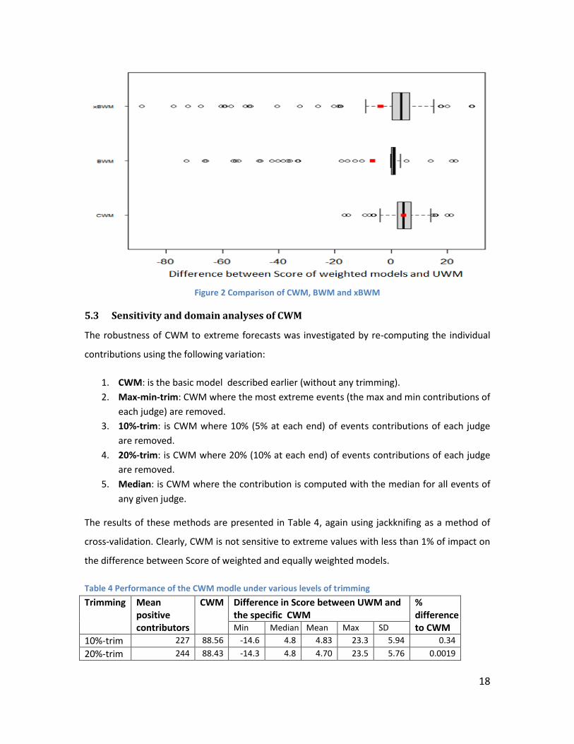
Figure 2 presents boxplots of difference between the Score of three weighted models

(CWM, BWM and xBWM) and the baseline model (UWM). The figure shows that there are less

outliers with CWM because the contribution score is in reference to the group and less about

individual performances, which have higher variances.

9 Percentage of impact = difference in Score between contribution and UWM/ difference in Score

between CWM and UWM

18

Figure 2 Comparison of CWM, BWM and xBWM

5.3 Sensitivity and domain analyses of CWM

The robustness of CWM to extreme forecasts was investigated by re-computing the individual

contributions using the following variation:

1. CWM: is the basic model described earlier (without any trimming).

2. Max-min-trim: CWM where the most extreme events (the max and min contributions of

each judge) are removed.

3. 10%-trim: is CWM where 10% (5% at each end) of events contributions of each judge

are removed.

4. 20%-trim: is CWM where 20% (10% at each end) of events contributions of each judge

are removed.

5. Median: is CWM where the contribution is computed with the median for all events of

any given judge.

The results of these methods are presented in Table 4, again using jackknifing as a method of

cross-validation. Clearly, CWM is not sensitive to extreme values with less than 1% of impact on

the difference between Score of weighted and equally weighted models.

Table 4 Performance of the CWM modle under various levels of trimming

Trimming Mean positive contributors

CWM Difference in Score between UWM and the specific CWM

% difference to CWM Min Median Mean Max SD

10%-trim 227 88.56 -14.6 4.8 4.83 23.3 5.94 0.34

20%-trim 244 88.43 -14.3 4.8 4.70 23.5 5.76 0.0019

19

Max-min- trim

228 88.39 -15.0 4.7 4.66 21.6 5.90 0.15

CWM 220 88.26 -16.7 4.4 4.53 21.5 5.41 ---

Median 291 87.72 -11.6 4.0 3.99 24.3 4.87 -0.61

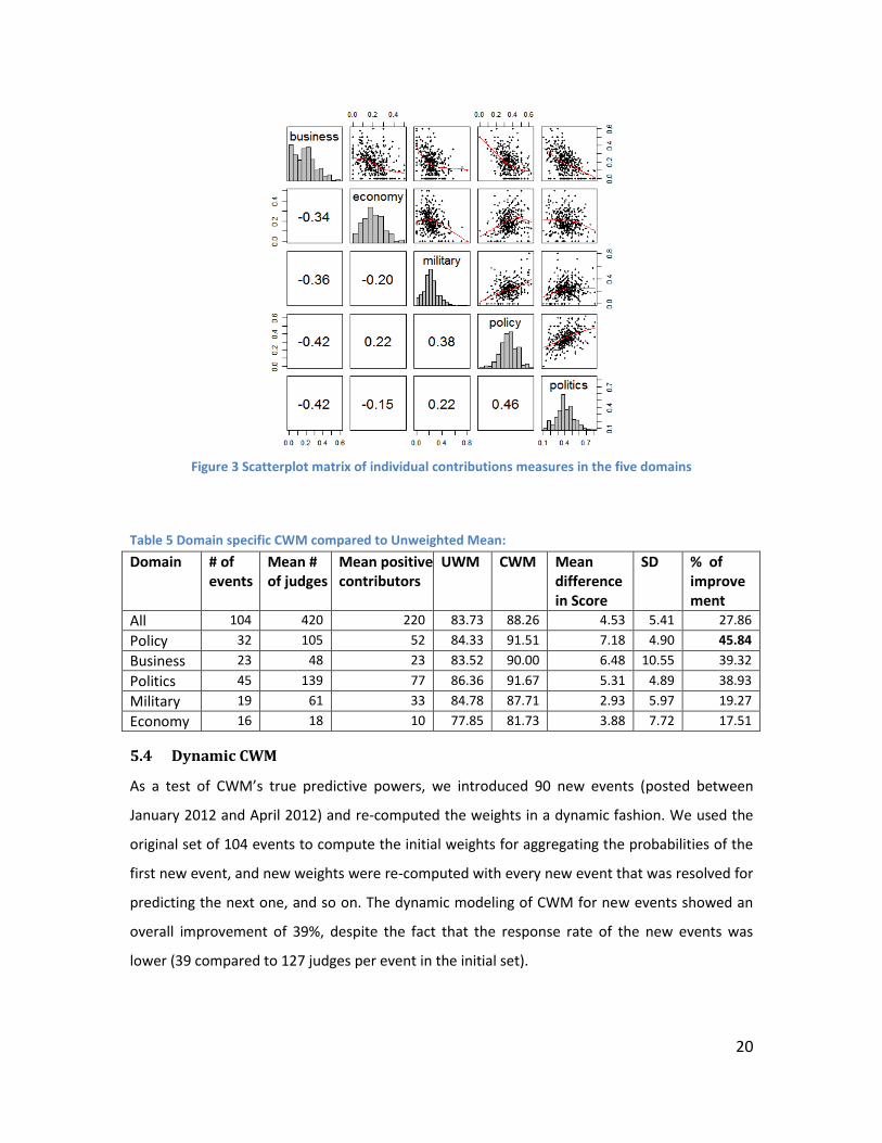
Contributions can be calculated separately for specific domains.. We applied the CWM

model to each of the 5 major domains separately again using only judges answering 10 or more

events in each domain, and cross-validated by jackknifing each event. Figure 5 shows positive

correlations between the domains, validating the interpretation of the Contribution as a

measure of expertise. Table 5 shows that the crowd (not necessarily the same judges in each

domain) performed better under the weighted than in the equally weighted model. The CWM

excelled, compared to the UWM, in the domain of policy with a 46% improvement (in bold) and

fared worst in economy with only an 18% improvement. The normalized average percent

improvement, based on the number of events, for the five domains is 35%. This cannot be

directly compared to the general model of 28% because some events were included in multiple

domains (note that the total number of events across the five domains is 135, which is greater

than the total number of events, 104)10, and the domain specific weights were calculated with a

threshold of 10 events for each domain.

10 For example, an item about military budget approval would count both as a military and policy

20

Figure 3 Scatterplot matrix of individual contributions measures in the five domains

Table 5 Domain specific CWM compared to Unweighted Mean:

Domain # of events

Mean # of judges

Mean positive contributors

UWM CWM Mean difference in Score

SD % of improvement

All 104 420 220 83.73 88.26 4.53 5.41 27.86

Policy 32 105 52 84.33 91.51 7.18 4.90 45.84

Business 23 48 23 83.52 90.00 6.48 10.55 39.32

Politics 45 139 77 86.36 91.67 5.31 4.89 38.93

Military 19 61 33 84.78 87.71 2.93 5.97 19.27

Economy 16 18 10 77.85 81.73 3.88 7.72 17.51

5.4 Dynamic CWM

As a test of CWM’s true predictive powers, we introduced 90 new events (posted between

January 2012 and April 2012) and re-computed the weights in a dynamic fashion. We used the

original set of 104 events to compute the initial weights for aggregating the probabilities of the

first new event, and new weights were re-computed with every new event that was resolved for

predicting the next one, and so on. The dynamic modeling of CWM for new events showed an

overall improvement of 39%, despite the fact that the response rate of the new events was

lower (39 compared to 127 judges per event in the initial set).

21

The dynamic model did better at the aggregate level, and the Score based on CWM was

better than the one based on the UWM in 71 out of 90 events (79%). This split is significantly

better than chance (50%) by a Wilcoxon signed rank test with p < 0.001. We also implemented

the dynamic model for each domain using the same recursive procedure. Table 6 summarizes

the results. The CWM improved the Score in all domains, except for economy, and the greatest

improvement was for military events. The superiority of the CWM over the UWM model was

significant in 3 of the 5 domains (military, politics and policy).

Table 6 Summary of the performance of the dynamic CWM for each domain:

6 Study 2: NFL Predictions

We seek to replicate the results from Study 1 in a different context involving predictions for the

National Football League (NFL) 2007 season. In this replication we apply CWM, as the model is

intended, in a purely dynamic setting while addressing three potential shortcoming of the ACES

dataset. We wanted to eliminate potential effects induced by: (1) the somewhat arbitrary

fashion in which events are forecasted whenever a judge chooses (i.e., in arbitrary order) which

events to predict and in what order by using a data set with a more rigid and systematic

temporal structure where all forecasters follow the same sequence for predicting games, (2)

the possibility of biases induced by the forecasters’ ability to select which events to predict, and

(3) the complexity associated with multiple domains. The intention is to show the rate at which

the metric of contribution can identify experts and CWM can produce an aggregate prediction in

comparison to a benchmark.

6.1 Data collection and simulations

Massey et al. (2011) invited NFL fans to complete weekly online surveys on the following week’s

NFL games. The NFL consists of 32 teams that play 16 games in the regular season over 17

Domain # of events

Mean # of judges

Mean positive contributors

UWM CWM Mean difference in Score

% of improvement

All 90 39.30 17.46 83.56 87.90 4.35 39.40*

Military 15 47.00 13.53 85.41 92.46 7.05 54.12*

Politics 49 36.80 14.84 84.26 91.13 6.87 53.36*

Policy 25 40.96 13.28 81.74 84.35 2.61 30.48*

Business 19 44.68 10.74 82.75 82.97 0.22 14.76

Economy 16 37.31 9.75 83.73 78.59 -5.15 -10.13

Note: * significant (α = 0.05) by a sign test

22

weeks. The sample is composed of 386 judges (45% female and 55% male, mean age = 35 years),

who completed more than 14 weeks of surveys. Each week they were asked to predict the

winning team and list the point differences (i.e., difference between the final score of the two

teams) for all games. They were also asked for their favorite team with a mean number of 12

participants per team (SD =3.57). They were awarded up to $3.50 per week based on the

average absolute difference between their predictions and the game outcomes, and the best

performer of the week was also given a $50 gift card.

Massey et al. (2011) found that the crowd was biased towards their “favorite” teams

more than “underdogs” and the bias increased over the four-month-long experiment despite

the obvious opportunity to learn with experience. The results illustrate a failure of that crowd’s

wisdom due to the systematic bias of the group to follow one’s pull towards the favorite teams

rather than learn from evidence.

We selected a subset of the Massey’s data set for our analysis. To control for favorite

team bias, 3 forecasters were randomly selected among those who identified a particular team

as their favorite. This yielded a sample of (31 teams x 3 judges =) 93 people (one team had only

one participant who picked it as their favorite).

The prediction of football scores is notoriously difficult (Winkler, 1971) with a base rate

of 64%11 for all games in this study compared to 18%12 for events in Study 1. In other words, a

judge answering based solely on these base rates would predict correctly (0.642 + -0.362) only

54% of the games. In contrast, in study 1 a judge answering based on the same principle would

predict correctly (0.182 + 0.822), i.e., 70% of the events. Another indication of this task’s

difficulty is the performance of the 93 judges in our sample. Their predictions have a mean

absolute error of 12.42 points (SD=9.72) with an average individual correlation of 0.21 (SD=0.08)

between the predicted and the actual scores.

11 This is the percentage of agreement between the official estimate at vegasinsider.com and the true

outcome of each game.

12 This is a percentage of the event occurring over the total number of events.

23

Given this obvious lack of “expertise” we decided to validate the CWM model by

simulating “experts”, combining them with the judges and testing if the model can identify

these experts and properly overweight them. For every judge (j), we generated a matched

expert (e) with a smaller error in the predicted point differences (point.diff). More precisely, for

each f the 244 games predicted by each judge, we calculated the absolute prediction error. In

those cases where it was greater than 15 (a value we selected to be 1.5 times the standard

deviation of the prediction errors) we reduced it to 15, preserving its direction When the error

was less than 15 we made no changes. Thus the experts’ predictions are never more than 15

points from the outcome of the game. The experts have a mean correlation between prediction

and outcome of 0.49 (SD=0.03), making them slightly better than the judges.

For the purpose of analysis, we created three mixed groups by replacing, in each case,

one of the three judges favoring each of the 31 teams in the sample with his / her expert

counterpart. Thus, each group is a combination of 62 original judges and 31 simulated experts,

for a total of 93 forecasters. The mean correlation between predictions and outcomes in the 3

mixed groups is 0.31 (SD=0.15).

Figure 4 presents boxplots of the individual correlations between the predictions and

outcomes of the games based on the judges, the experts, and the three mixed groups

Figure 4 Boxplots of correlation analyses for judges and experts

24

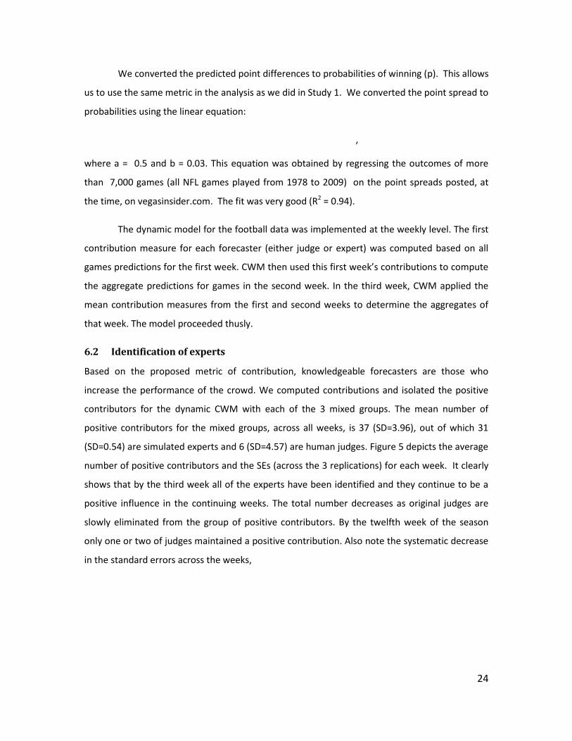
We converted the predicted point differences to probabilities of winning (p). This allows

us to use the same metric in the analysis as we did in Study 1. We converted the point spread to

probabilities using the linear equation:

,

where a = 0.5 and b = 0.03. This equation was obtained by regressing the outcomes of more

than 7,000 games (all NFL games played from 1978 to 2009) on the point spreads posted, at

the time, on vegasinsider.com. The fit was very good (R2 = 0.94).

The dynamic model for the football data was implemented at the weekly level. The first

contribution measure for each forecaster (either judge or expert) was computed based on all

games predictions for the first week. CWM then used this first week’s contributions to compute

the aggregate predictions for games in the second week. In the third week, CWM applied the

mean contribution measures from the first and second weeks to determine the aggregates of

that week. The model proceeded thusly.

6.2 Identification of experts

Based on the proposed metric of contribution, knowledgeable forecasters are those who

increase the performance of the crowd. We computed contributions and isolated the positive

contributors for the dynamic CWM with each of the 3 mixed groups. The mean number of

positive contributors for the mixed groups, across all weeks, is 37 (SD=3.96), out of which 31

(SD=0.54) are simulated experts and 6 (SD=4.57) are human judges. Figure 5 depicts the average

number of positive contributors and the SEs (across the 3 replications) for each week. It clearly

shows that by the third week all of the experts have been identified and they continue to be a

positive influence in the continuing weeks. The total number decreases as original judges are

slowly eliminated from the group of positive contributors. By the twelfth week of the season

only one or two of judges maintained a positive contribution. Also note the systematic decrease

in the standard errors across the weeks,

25

Figure 5 Average number of judges and simulated experts with positive contributors per week

The influence of judges (mean=0.08, SD=0.02) also decreases with the passing weeks as

their weights in the contribution model approached zero, while the opposite effect is observed

for experts (mean=0.94, SD=0.01). Figure 6 illustrates that by the third week 90% of the weights

for the model come from the experts.

Figure 6 Sum of weights for positive contributors for judges and simulated experts per week

In essence, the metric of contribution not only identified the consistently knowledgeable

forecasters, but the variance of contribution also decreased as more information is gathered.

Using only positive contributors diminished the effect of chance over time, and skill emerged

from the model.

6.3 Impact of expertise and diversity on CWM

26

One benefit of simulating experts is the ability to create different groups whose comparison

allows us to test the CWM. We ran the model using (1) only the original judges, (2) only the

simulated experts, and (3) a combination of the two (with expert to judge ratio of 1:2). Figure 7

shows the resulting mean Scores of the judges, experts and average of the mixes for the season.

The average mix group produced a mean Score of 82.79 (SD = 2.97) much closer to that of the

experts (mean=83.63, SD=3.05) than that of the original judges (mean=77.20, SD=3.03). In fact,

CWM of the mixes generated aggregate forecasts in the initial week of prediction almost as

accurate as a benchmark CWM of experts. This pattern of a close match between CWMs of the

average mix and experts is stable over time.

Figure 7 CWM Scores for experts, judges and mix across weeks

The CWM is a composite model that first computes individual contributions and then

uses them to weigh predictions. It is natural to test which of these two stages drives the

performance of the model. The mean improvement in prediction (relative to the unweighted

mean, UWM) for (a) the simple average of positive contributors with no differential weighing

(contribution) was 2.41 (SD=0.57, α < 0.05) or 11.95%, and (b) the differential weighing (CWM)

was 2.98 (SD=0.74, α < 0.05) or 14.77%. Clearly, the strength of the model is derived mostly

from identifying the positive contributors, with 81% of CWM’s improvement over UWM due to

contributions, rather than weighing their predictions.

Although positive contributors have a significant effect on the average mix group (15%

improvement from UWM to CWM), this was not observed in the homogenous groups of experts

(4% improvement) and judges (2% decline). Figure 8 depicts the mean Score for UWM,

27

contribution and CWM for experts, judges and the average mix group. It shows that diversity in

the heterogeneous group allowed significant improvement of Score by the model and that most

of the impact is attributed to identifying positive contributors.

Figure 8 Comparison of models for experts, judges and mix

7 General Discussion

There are two distinct approaches in the quest for the most accurate probabilistic forecasts.

One approach seeks individual expertise, and the other seeks to aggregate multiple opinions

from a crowd without paying much attention to its individual members. The key ideas of WOC

are that the aggregation process can reduce the effects of individual biases, and that one can

use the central tendency of the crowd’s opinions to forecast the target events. We suggest a

new approach that combines the two philosophies by (a) identifying the experts in the crowd

and (b) averaging their opinions, while ignoring the estimates of the non-experts. In a sense this

can also be seen as a compromise between the two approaches. The major technical

contribution of the current paper is the new measure for identifying experts in a crowd by

measuring their contribution to the crowd’s performance.

We often assume that expertise can be identified simply by relying on past performance

on similar tasks. Indeed, if the at some point in the process one would be asked to choose a

single expert, we cannot think of a way of selecting an expert that would beat this intuitive

metric of absolute quality of performance. However, if one continues to rely on a crowd (or at

28

least a subset of its members), our results show that one can do considerably better by relying

on the proposed measure of relative quality. We illustrated this approach in two longitudinal

studies. By isolating the experts (those who make positive contributions to the crowd), the

mean Brier scored improved by 17% in Study 1 and 12% in Study 2 compared to the average of

the crowd. The weighted model (CWM) implemented with positive contributors furthered

improved performance by 28% in Study 1 and 15% in Study 2. This is not to say that every event

predicted in Study 1 was improved by using only the reported probabilities of these experts, but

over time, the variance decreased and the model proved overall significant better than the

simple (unweighted) mean(s) and weighted means relying on past performance. Our selection of

experts is not based on the best performers (highest Scores) because their performances can be

skewed by one or a few extreme predictions (Denell & Fang, 2010). We pick those who have

consistently outperformed the group, and our model is updated dynamically to reduce variance

due to chance results and to reflect “true” expertise that emerges in the process. This is best

observed in the analysis of the NFL games where we can trace how well and how quickly the

simulated experts rise to the top.

The success of our approach is quite intuitive, once one realizes that judges are usually

highly correlated (see Broomell & Budescu, 2009) because they share certain assumptions

and/or have access to the same information. Consequently, crowds often behave like herds as

almost everyone expects certain events to happen (or not). This can backfire when the

assumptions are false and/or the information is incomplete or biased. A good example is the

recent case when prediction markets’ “failed” to predict the US Supreme Court’s decision

regarding the Affordable Care Act (Prediction markets estimated a 75% chance that it would not

be upheld by the court). Our contribution metric identifies and over weights the predictions of

those judges who do not necessarily follow the crowd in such cases and helps avoid such traps.

An interesting theoretical issue is what makes the CWM work – its ability to identify the

experts or their differential weighting. Results from both studies clearly suggest that it is

primarily the model’s ability to identify the experts to be positively weighted (or, in other words,

its ability to identify those members of the crowd who should be excluded), that are responsible

for most of the model’s improvement. This is not surprising, as the relative insensitivity of the

model to departures from optimal weighting is well recognized in the literature (e.g., Broomell &

Budescu, 2009; Davis-Stober, Dana & Budescu, 2010; Dawes, 1979).

29

Sensitivity analyses confirmed the robustness of the CWM model, as its performance

was largely unaffected by various degrees of trimming. Three analyses support the validity of

the approach: (1) the model clearly outperformed randomly simulated responses with matching

means and variances (Model betaCWM in Study 1); (2) its performance improved when it was

applied separately to various domains of expertise in Study 1; and (3) the model was able to

identify – almost perfectly and very rapidly – the simulated experts in Study 2. All three results

indicate that the contribution measures we extract reflect real expertise.

The dynamic implementation of CWM is, probably, the most attractive feature from a

practical point of view. Our results demonstrate that the CWM can easily adapt to new events

and games (producing 39% improvement over UWM in Study 1 and 15% in Study 2) by including

new experts or discarding old ones as their mean contribution changes. For Study 1, the

dynamic model was especially useful in correlated domains like military, policy and politics

(where predictions enhanced by 54%, 53% and 31% respectively) for judges possessing

knowledge that was adaptable to all three. The model improves as more information is gathered

by reducing the variance that is associated with chance success to distil the true experts from

the crowd, as shown by the frequency (Figure 5) and weights (Figure 6) of experts and judges for

positive contributors in the mix groups over time. By benchmarking CWM to a model including

only experts in Study 2, we observed that the predictions of the CWM model were almost as

good as those of the “ideal” model. Clearly, the model can be applied successfully in continuous

and longitudinal setups, even in sparse cases (as in Study 1).

8 Conclusion

We proposed a new measure of individual contribution that is simple, reliable, easily interpreted

and useful for assessing forecaster’s performance relative to the crowd. We tested our model in

two contexts, and it both cases it outperformed models built solely on past, individual

performance and on the simple average of the crowd. The model gets its power mostly by

identifying experts who have consistently outperformed the crowd. It works well when there is

longitudinal data even if in cases of sparse data, and it identifies the experts relatively quickly.

References

30

Armstrong, J. S. (2001). Principles of forecasting: A handbook for researchers and practitioners. Kluwer Academic, Boston, MA.

Ariely, D., W.T. Au., R.H.Bender, D.V.Budescu, C.Dietz, H.Gu, T.S. Wallsten, G. Zauberman. (2000). The effects of averaging subjective probability estimates between and within judges. J. Experimental Psych.: Applied 6(2) 130-147.

Bedford, T., R. Cooke. (2001). Probabilistic Risk Analysis: Foundations and Methods. Cambridge University Press, Cambridge, UK.

Bettman, J. R., M. F. Luce, J.W. Payne. (1998). Constructive consumer choice processes. J. Consumer Res. 25 (2) 187–217.

Bickel, E. (2007). Some comparisons among Quadratic, Spherical, and Logarithmic scoring rules. Decision Analysis 4(2) 49-65.

Bordley, R. (2011). Using Bayes' rule to update an avent's probabilities based on the outcomes of partially similar events. Decision Analysis 8(2) 117-127.

Brier, G. W. (1950). Verification of forecasts expressed in terms of probability. Monthly Weather Rev. 78(1) 1–3.

Broomell, S, D.V. Budescu. (2009). Why are expert correlated? Decomposing correlations between judges. Psychometrika 74(3) 531-553.

Budescu, D. V. (2006). Confidence in aggregation of opinions from multiple sources. K. Fiedler, P. Juslin, eds. Information sampling and adaptive cognition. Cambridge University Press, Cambridge, UK, 327-352.

Budescu, D.V., A.K. Rantilla. (2000). Confidence in aggregation of expert opinions. Acta Psychologica 104(3) 371-398.

Budescu, D.V., H.Y. Yu. (2006). To Bayes or not to Bayes: A comparison of two classes of models of information aggregation. Decision Analysis 3(3) 145-162.

Clemen, R. T. (2008). Improving and measuring the effectiveness of decision analysis: Linking decision analysis and behavioral decision research. T. Kugler, J. C. Smith, T. Connolly, Y.-J. Son, eds. Decision modeling and behavior in complex and uncertain environments . Springer, New York, 3-31.

Clemen, R. T. (1989). Combining forecasts: A review and annotated bibliography. International Journal of Forecasting 5(4) 559-609.

Clemen, R. T., R. L. Winkler. (1999). Combining probability distributions from experts in risk analysis. Risk Analysis 19(2) 187-203.

Clemen, R. T., R. L. Winkler. (1990). Unanimity and compromise among probability forecasters. Management Science. 36(7) 767-779.

Clemen, R. T., R. L. Winkler. (1986). Combining economic forecasts. Journal of Business and Economic Statististics. 4(1) 39-46.

31

Cooke, R.M. (1991). Experts in Uncertainty. Oxford University Press, Oxford, UK.

Cooke, R.M., L.H.J.Goossens. (2007). TU Delft expert judgement database. Reliability Engineering and System Safety 93(5) 657–674.

Davis-Stober, C., J.Dana, D.V. Budescu, (2010). A constrained linear estimator for multiple regression. Psychometrika, 2010, 75, 521-541.

Davis-Stober, C., D.V. Budescu, J.Dana, S.Broomell. (2012). When is a crowd wise? Paper submitted for publication.

Dawes, R. M. (1979).The robust beauty of improper linear models in decision making. Ameican Psychologist 34(7) 571-582.

Denrell, J., C.Fang. (2010). Predicting the next big thing: Success as a signal of poor judgment. Management Science 56(10) 1653-1667.

Evgeniou, T., L. Fang, R.H. Hogarth, N.Karelaia. (2012). Competitive dynamics in forecasting: The interaction of skill and uncertainty. Journal of Behavioral Decision Making (forthcoming – published online July 2012).

French., S. (2011). Expert judgement, meta-analysis and participatory risk analysis. Decision Analysis 9(2) 119-127.

French, S. (1985). Group consensus probability distributions: a critical survey. J.M. Bernardo,

M.H. DeGroot , D.V.Lindley, A.F.M. Smith, eds. Bayesian Statistics, vol. 2, North-Holland, Amsterdam, 183-201.

Gaissmaier, W., J. N. Marewski. (2011). Forecasting elections with mere recognition from small, lousy samples: A comparison of collective recognition, wisdom of crowds, and representative polls. Judgment and Decision Making 6(1) 73–88.

Galton, F. (1907). Vox Populi. Nature 75(March) 450–51.

Genest, C., J.V. Zidek. (1986). Combining probability distributions: a critique and annotated bibliography. Statistical Science 1(1) 114-148.

Gilovich, T., D. Griffin, D. Kahneman. (2002). Heuristics and Biases: The Psychology of Intuitive Judgment. Cambridge: Cambridge University Press.

Hastie, R., T. Kameda. (2005). The robust beauty of majority rules in group decisions. Psychological Review 112(2) 494-508.

Hertwig, R. (2012). Tapping into the Wisdom of the Crowd—with Confidence. Science 336 (6079) 303-304

Herzog, S.M., R. Hertwig. (2011). The wisdom of ignorant crowds: Predicting sport outcomes by mere recognition. Judgment and Decision Making 6(1) 58–72

Herzog, S.M., R. Hertwig. (2009). The wisdom of many in one mind: Improving individual judgments with dialectical bootstrapping. Psychological Science 20(2) 231-237.

32

Hogarth, R.M. (1978), A note on aggregating opinions. Organizational Behavior and Human Performance 21 (1) 40–46.

Jain, K., J.N. Bearden, A. Filipowicz. (2011). Diverse personalities make for wiser crowds: How personality can affect the accuracy of aggregated judgments. (working paper).

Kahneman, D., A. Tversky. (2000). Choices, Values,and Frames, New York: Russell Sage Foundation.

Koriat, A. (2012). When are two heads better than one and why?, Science 336(6079) 360-362. Kutner, M.H., C. J. Nachtsheim, J. Neter, W. Li. (2005). Applied Linear Statistical Models, (5th

ed), McGraw Hill Irwin. Johnson, T.R., D.V. Budescu, T.S. Wallsten. (2001). Averaging probability judgments: Monte

Carlo analyses of asymptotic diagnostic values. Journal of Behavioral Decision Making, 14(2) 123-140.

Larrick, R.P., A.E. Mannes, J.B. Soll. (2011). The social psychology of the wisdom of crowds. In

Krueger, J. I. (Ed.), Frontiers in social psychology: Social judgment and decision making. New York: Psychology Press.

Larrick, R.P., J.B. Soll. (2006). Intuitions about combining opinions: Misappreciation of the

averaging principle. Management Science 52(1) 111-127.

Lee, M. D., S. Zhang, J. Shi. (2011). The Wisdom of the crowd playing the Price is Right. Memory & Cognition 39(5) 914-923

Lin, S.-W., C.-H. Cheng. (2009). The reliability of aggregated probability judgments obtained through Cooke’s classical model. Journal of Modelling in Management 4(2), 149–161.

Lorenz, J., H. Rauhutb, F. Schweitzera, D. Helbing. (2011). How social influence can undermine

the wisdom of crowd effect. Proceedings of the National Academy of Science 108(2) 9020–9025.

Makridakis, S., R.L. Winkler. (1983). Averages of forecasts: Some empirical results. Management Science 29(9) 987-996.

Massey, C., J. Simmons, D.A. Armor. (2011). Hope over experience: Desirability and the persistence of optimism, Psychological Science 22(2) 274 - 281.

McCrae, R.R., O.P. John. (1992). An introduction to the five-factor model and its applications. Journal of Personality 60(2) 175-215.

Miller, B., M. Steyvers. (2012). The wisdom of crowds with communication. In L. Carlson, C. Hölscher, & T.F. Shipley (Eds.), Proceedings of the 33rd Annual Conference of the Cognitive Science Society. Austin, TX: Cognitive Science Society.

33

Phillips, L.D. (2007). Decision conferencing. In Edwards,W., Miles, R.F., vonWinterfeldt, D. (Eds) Advances in Decision Analysis: From Foundations to Applications, Cambridge University Press, Cambridge. 375–399.

Rowe, G., G. Wright. (2001). Expert opinions in forecasting: The role of the Delphi Technique. In J. Armstrong (Ed.). Principles of Forecasting. Boston: Kluwer Academic. 125-144

Simmons, J., L. D. Nelson, J. Galak, S. Frederick. (2011). Intuitive biases in choice vs. estimation: Implications for the wisdom of crowds, Journal of Consumer Research 38(1) 1 - 15.

Simonson, I. (1989). Choice based on reasons: The case of attraction and compromise effects. Journal of Consumer Research 16(2) 158–174.

Sniezek, J.A., R.A. Henry. (1989). Accuracy and confidence in group judgment.Organizational Behavior and Human Decision Processes 43(1) 1-28.

Soll, J.B., R.P. Larrick. (2009). Strategies for revising judgment: how (and how well) people use others’ opinions, Journal of Experimental Psychology: Learning, Memory and Cognition 35(3) 780–805.

Sunstein, C.R. (2006), Infotopia: How many minds produce knowledge, New York: Oxford University Press.

Surowiecki, J. (2004). The wisdom of crowds: Why the many are smarter than the few and how collective wisdom shapes business, economies, societies, and nations. London: Little, Brown.

Tetlock, P.E. (2005) Expert Political Opinion, How Good is it? How Can we Know? Princeton, Princeton University Press.

Wallsten, T.S., D.V. Budescu, I. Erev, A. Diederich. (1997). Evaluating and combining subjective probability estimates. Journal of Behavioral Decision Making 10(3) 243-268.

Wallsten, T. S., D.V. Budescu, R. Zwick. (1993). Comparing the calibration and coherence numerical and verbal probability judgments. Management Science 39(2) 176-190.

Wallsten, T.S., D.V. Budescu. (1983). Encoding subjective probabilities: A psychological and psychometric review. Management Science 29(2) 151-173.

Wallsten, T.S., A. Diederich. (2001). Understanding pooled subjective probability estimates. Mathematical Social Science 41(1) 1-18.

Wang, G., S.R. Kulkarni, H.V. Poor, D.N. Osherson. (2011). Aggregating large sets of probabilistic forecasts by weighted coherent adjustment. Decision Analysis 8(2) 28–144.

Yaniv, I. (2004). Receiving other people's advice: Influence and benefit. Organizational Behavior and Human Decision Processes 93(1) 1-13.

Acknowledgments:

34

This work was supported, in part, by the Intelligence Advanced Research Projects Activity

(IARPA) via Department of Interior National Business Center contract number D11PC20059.

We thank Dr Cade Massey and his colleagues for allowing us to re-analyze their NFL prediction

results

35

Appendix: Correlation analyses of contribution

We computed individual contributions to the crowd for the 420 judges. Note that in this case

each judge’s contribution is based only on the subset of events he / she answered (which varies

in size – as shown in Table 2 – and its composition across judges). As expected, about half of the

judges (220) had positive contributions. The mean contribution is 0.004 and the standard

deviation is 0.089. Figure 9 depicts a scatter matrix of 8 variables: contribution score, Score, the

number of events answered, self-reported knowledge, self-reported time spent reading the

news, timing for answering events, education, and years of experience. Most correlations are

low. As anticipated, the strongest correlation was found between contribution and mean SCORE

of judges (r=0.75). Some mild correlations were also present between timing and other variables

such as contribution (r=0.10), the number of events answered (r=0.21), and years of experience

(r=0.11). Most participants answered events closer to the opening dates, which can be due to

the email alerts that they received when new events are introduced on the site. People with less

experience answered at the opening of the event and those with more experience tended to

answer later. Judges with high contribution scores also tended to answer near the closing date.

Some of the self-reported measures are also correlated, such as education with SCORE (r=0.13)

and years of experience (r=0.10), knowledge with years of experience (r=0.12). Additionally, the

more educated is the participant the more events they answered (r=0.12).

In principle, the later a forecast is submitted relative to the timing of the event, the

more accurate (high Score) it should be, based on the fact that the forecasters have access to

more information with time. To investigate the effect of timing of answers on contribution, we

correlated the two variables for each of the 420 judges, across all the events they answered13.

Figure 10 shows a histogram and boxplot of the distributions for the 420 correlations. The mean

value for the distribution in Figure 10 is -0.0658, describing virtually no correlation between

timing and contributions for the judges.

13 This differs from the analysis described in Figure 9, where the correlation is based on the mean

contribution and mean timing for each judge.

36

Figure 9 Scatterplot matrix14

of correlation for overall descriptive statistics.

14 Missing values for self-reported measures are represented on the last column of each plot.

37

Figure 10 Histogram combined boxplot of correlations for timing and contributions

Correlation of timing vs. contribution