identifying key sectors for green growth in india: an

! 1!

Identifying key sectors for Green Growth in India: An Environmental Social Accounting Matrix multiplier

analysis

Barun Deb Pal, Assistant Professor,

Institute for Social and Economic Change, Bangalore, India,

[email protected]

Abstract

This paper has adopted method of Environmental Social Accounting Matrix (ESAM) and its multiplier to construct a sector specific green growth index to identify key sector for green growth in India. This index comprises of sector wise implications on GDP growth, growth in employment, income growth, GHG emissions and energy use. Results of this analysis show that the cereal productions other than rice and wheat can be given higher priority to promote green economic growth. Meanwhile the hydro electricity production will be in high priority for this followed by other industrial activities. Finally this study has shown that the existing pattern of government expenditure is sub-optimal as its reallocation based on their green growth index increases GDP by 1%, reduces GHG emission by 1.57% and increase employment by 2.57%.

Key words: SAM, Environment and growth, GHG,

JEL Classification: E16, Q44, Q54,

! 2!

1. Introduction

At the outset, green growth has become the centre piece of development strategy of many

countries including India. The recently released 12th Five Year Plan document of India has

talked at length on achieving economic growth concomitant with conservation of natural

resources, minimising environmental pollution, promotion of clean source of energy and

improvement in energy efficiency in all sectors. It has budgeted substantial fund for

improving environment. However, the plan document has been silent regarding the

quantification of the environmental impact of various sectoral investment goals. Nor it has

been attempt to justify whether the target growth rate (9% during the period 2012-17) would

be achieved with minimum environmental damage.

Given the importance of green growth, many countries nowadays produce environmentally

extended social accounting matrix (ESAM) so that one can quantify the environmental effect

of desired sectoral investment or growth1. Since ESAM is an extension of a Social

Accounting Matrix (SAM), the multiplier derived from ESAM will produce direct and

indirect induced impact of the policies on economic growth and environment, which may be

used for understanding sectoral impact of investment/growth on environment. To our best

knowledge, no attempt has been made to construct ESAM for India.

Therefore, this study is an attempt to construct an ESAM for India. The multiplier analysis

derived from the ESAM would enable us to estimate various multipliers to see the direct and

indirect induced consequences of a sector on various economic and environmental indicators.

However, the selection of multiplier depends on the developmental perspective considered by

the researcher. Since our key focus is green growth for Indian economy, various multipliers

effects derived from ESAM have been integrated together to estimate sector specific Green

!!!!!!!!!!!!!!!!!!!!!!!!!!!!!!!!!!!!!!!!!!!!!!!!!!!!!!!!!!!!!1 The countries for which these are available are Netherlands, Bolivia, Chile, China and UK (Keuning (1992); Alarcon, van Heemst and de Jong (2000); Gallardo and Mardones (2013); Jian Xie (2000); Stanislav Edward Shmelev (2010)).

! 3!

Growth Index (GGI) for India. Such analysis enables us to understand key sector for green

growth in India. Again as the green growth is common but differentiated responsibility of

every country across the world, such analysis would help in policy making process for India.

Following this introductory sections, the rest of the paper is organised as follows. The section

2 describes conceptual framework of our proposed ESAM for India. The sectoral scheme and

construction procedure is described in section 3. The section 4 demonstrates the derivation of

ESAM multiplier and section 5 describes application of ESAM multiplier to estimate GGI for

India to identify key sectors for green growth. Section 6 describes an illustrative example of

ESAM multiplier model in policy making process. As a part of this, we have analysed the

impact of fiscal reallocation on economic growth as well as GHG emissions in India. Finally

section 7 gives some concluding remarks of this study.

2. Environmentally Extended Social Accounting Matrix (ESAM): Framework

The structure of our proposed ESAM followed from the National Accounting Matrix

including Environmental Accounts (NAMEA) for the Netherlands for the year 1992

(Keuning, S. J. 1992). Like NAMEA our proposed ESAM also takes into account a

substances account, and an account for environmental themes as an extension of a Social

accounting matrix of India. The detail structure of this ESAM is described in the following

Table 12.

!!!!!!!!!!!!!!!!!!!!!!!!!!!!!!!!!!!!!!!!!!!!!!!!!!!!!!!!!!!!!2!See!Keuning,!S.!J.!(1992),!for!detail!description!about!the!NAMEA!structure!

! 4!

Table 1: Schematic Structure of Environmentally Extended Social Accounting Matrix

Production Factors of production

Institutions Indirect taxes

capital account

Rest of the world

Substances (GHG) Depletion of Natural resource

Env.theme

Renewal of Energy resource

Renewal of land

1 2 3 4 5 6 7 8 9 10

Production 1 Intermediate consumption

Consumption of goods and services

Change in stocks and capital formation

Exports Emission of pollutants from production

Factors of production

2 Payment for factors

Net factor income from abroad

Discovery of Energy capital

Renewal in land through conservation

Institutions 3 Value added income Transfer from other institutions

Total tax receive

Net current transfers

Emission of pollutants from consumption

Indirect taxes 4 Taxes on intermediate

Taxes on purchase Taxes on investment

capital account 5 Depreciation Savings Foreign savings

Rest of the world 6 Imports

Substances (GHG) 7 Absorption of substances in production

Absorption of substances in consumption

Accumulation of substances

Depletable Substances

Depletion of Energy Resources

8 Extraction of Energy stock

Net Reduction in natural stock

Depletion of Land

9 Depletion of land due to land use change

Emission from land use change

Net depletion in land

Env.theme GHG inventory

! 5!

3. Sectoral Scheme and method of construction

At the outset, the core of an ESAM/SAM is the input output table and supplementary

environmental data. Since the input-output table for India is available for the year 2006-

07, we have chosen 2006-07 as the base year of the ESAM.3 The input-output table for

the year 2006-07 gives inter-industry flow for 130 sectors of the Indian economy.

However, the relevant data are not available for all the 130 sectors of the Indian

economy to construct an ESAM for India. Therefore, we have decided to take into

account broad sectors on the basis of their energy and emission intensities. Also we

have decided to model different types of energy and electricity production sectors as

separate entities since the same are relevant for climate change analysis. We have

grouped these 130 production sectors into 35 production sectors to construct ESAM for

India for the year 2006-07. Our ESAM incorporates 3 factors of production and 9

categories of occupational households. Table 2 gives the description of ESAM sectors

and its concordance with 130 sectors of the input-output table while Table 3 gives

description of households’ classes.

Table 2: Map of Concordance between ESAM sectors and sectors of Input-Output

Table

Serial No.

Sector Code

Sectors for SAM Sectors of IO table 2006-07

1 PAD Paddy Rice 1 2 WHT Wheat 2 3 CER Cereal, Grains etc, other crops Part of (3-7,18,19, 20) 4 CAS Cash crops 8,9,10-17 5 ANH Animal husbandry & prod. Part of (21, 22, 23, 24) 6 FOR Forestry Part of 25 7 FSH Fishing 26 8 COL Coal 27 9 OIL Oil 29

!!!!!!!!!!!!!!!!!!!!!!!!!!!!!!!!!!!!!!!!!!!!!!!!!!!!!!!!!!!!!33!Recently!an!input/output!table!for!2007/08!has!been!published.!However,!other!required!environmental!data!are!not!available!for!2007/08.!So,!we!have!constructed!ESAM!for!the!year!2006/07.!

! 6!

Serial No.

Sector Code

Sectors for SAM Sectors of IO table 2006-07

10 GAS Gas 28 11 MIN Minerals n.e.c. 30-37 12 FBV Food & beverage Part of (38-45) 13 TEX Textile & Leather 46-54, 59, 60 14 WOD Wood 56 15 PET Petroleum & Coal Prod. 63,64 16 CHM Chemical, Rubber & Plastic prod. 58,61,62,65,66, 69-73 17 PAP Paper & Paper prod. Part of 57 18 FER Fertilizers & Pesticides 67,68 19 CEM Cement 75 20 IRS Iron & Steel 77,78, 79 21 ALU Aluminum 80 22 OMN Other manufacturing 55, 74, 76, 81, 82, 95-105 23 MCH Machinery 83-94 24 HYD Hydro 107 25 NHY Thermal 107 26 NUC Nuclear 107 27 BIO Biomass Part of (3-7,18,19, 20), Part of (21, 22, 23,

24), Part of 25, Part of (38-45), Part of 57

28 WAT Water 108 29 CON Construction 106 30 LTR Land transport 110, 113 31 RLY Rail Transport 109, 113 32 AIR Air Transport 112, 113 33 SEA Sea Transport 111, 113 34 HLM Health & medical 122 35 SER All other services 114-121, 123, 124-126, 127-130

Table 3: Households and other Institutions of ESAM

Agent code Description

RNASE Rural non-agricultural self employed

RAL Rural agricultural labour

ROL Rural other labour

RASE Rural agricultural self employed

ROH Rural other households

USE Urban self employed

USC Urban salaried class

UCL Urban casual labour

UOH Urban other households

! 7!

3.1. Method of Constructing ESAM of the year 2006-07

The method of constructing ESAM has two parts, namely construction of the SAM and

extension of SAM with environmental indicators. To construct SAM for India, we have

followed the same methods described in the paper by Pal, Pohit and Roy (2012) (see

Figure 1 for successive steps).

Figure 1: Construction procedure of SAM

!

Extend 130 sector commodity X commodity IO tale with hydro, non-hydro, nuclear, biomass and road transport non-motorised sectors.

Aggregate the extended IO table with the help of the concordance map

Decomposition of sector wise gross value added (GVA) into labour, capital and land income and also estimate net labour income and capital income from abroad.

!

Decompose services Incidental to transport sector according to the transport sector on which this services are associated

Estimate capital account to show savings and investment of the economy

Consider 130 sectors commodity X Commodity IO table for India for the year 2006-07 from central statistical organization of India

Distribute! private! final! consumption! expenditure! (PFCE)! and! the! total! indirect! taxes!

imposed!on!household!final!consumption!among!the!household!classes.!

!

Estimate!direct!taxes!paid!by!the!different!household!classes!

Estimate factor income, transfer income (domestic & foreign), tax income (for government only) and income from public debt for the 12 institutions.

! 8!

Primarily we have followed government official sources to obtain relevant data for

extending input output table for SAM. Additionally, we have followed the data

available in previous SAMs of India published by various researchers.

Once we constructed 35 sectors SAM for India for the year 2006-07, our next step is to

extend this SAM to construct ESAM for India. The method of extension is given in the

following Figure 2.

Figure 2: Extension of SAM to construct ESAM

Consider!35!sector!SAM!!

Extended!with!Environmental!

substances!account!!

Extended!with!Environmental!theme!

account!!

Damaging!Substances! Depletable!substances!!

Row!of!damaging!

substances!!

Column!of!damaging!

substances!!

Estimate!GHG!absorptions!

by!production!sectors!!

Estimate!GHG!emissions!

from!production!sectors!!

Row!of!depletable!

substances!!Column!of!depletable!

substances!!

Estimate!depletion!of!

natural!resources!!

Estimate!Renewal!of!

natural!resources!!

Row!of!GHG!emission!

inventory!

Column!of!Sector!specific!

Gross!GHG!emission!

! 9!

To complete the construction of ESAM for India, we have to estimate sector specific

data as mentioned in Figure 3. Below, we have described detailed method of estimating

sector specific data for ESAM for India.

3.2!Estimation of Environmental Data!!!!

As noted earlier, our focus is to capture GHG emissions in our ESAM. To estimate

column and row of damaging substances accounts, we have estimated sector wise

emission and absorption of GHGs for the Indian economy. Additionally we have

attempted to incorporate depletion and renewal of natural resources like; coal, crude oil

and land in our ESAM and the relevant data need to be sourced.

3.2.1 Estimation of sector specific GHG emissions

India has published its second communication on greenhouse gas emission, which

provides updated information on India’s greenhouse gas emission from different sectors

for the year 2007 (MOEF, 2010). The same source is used to estimate India’s sector

specific GHG emissions for the year 2007. Since our sectors do not exactly match with

that of MOEF report, we have derived a concordance between the two which is given in

Table 5.

Table 4: Mapping between ESAM sector and sector of MOEF report

Sector of ESAM MOEF Sectors Pddy rice Agriculture, Rice Cultivation, soils Wheat Agriculture, soils Cereals Agriculture, soils Cash crops Agriculture, soils Animal husbandry Agriculture, Enteric fermentation, Manure management Forestry No emission Fishing Agriculture Coal Fugitive Emission Oil Fugitive Emission Gas Fugitive Emission Food & Beverages Food Processing, Industrial waste water Textiles & Leather Textile & Leather, Industrial waste water

! 10!

Sector of ESAM MOEF Sectors Wood Non-specific industries Minerals n.e.c Mining & qurrying Petroleum & Coal tar product Other energy Industry, Industrial Waste water Chemical, Rubber & Plastic Products Chemicals, Industrial waste water Paper & Paper products Pulp & paper, Industrial waste water Fertiliser & Pesticides Non-specific industries, Industrial waste water Cement Cement Iron & steel Iron & steel Aluminum Aluminum Other manufacturing Ferroalloys, Lead, Zinc, Copper, Glass & cermic, soda

ash, Non-specific industries Machinery Non-specific industries, Industrial waste water Thermal Electricity, Industrial waste water Hydro No emission Nuclear No emission Biomass No emission Water No emission Construction Non-specific industries Land transport Road Transport Railway transport Railways air transport Aviation Water transport Navigation Health and medical No emission Other services Commercial /Institutional !

Since the concordance map indicates absence of one to one correspondence between the

two in many sectors, we need to derive a scheme to disaggregate the GHG emissions for

the MOEF sectors. The method of disaggregation is described in the following Table 5.

! 11!

Table 5: Method of disaggregating source wise GHG emissions in India

Corresponding sector Items to be disaggregated CO2 N2O CH4 Paddy, Wheat, cereals, cash crop and fishing

Energy based emission from Agriculture sector

Petroleum Fuel consumption shares have been used

N.A N.A

Same as above Emission from Soil N.A Fertilizer Consumption shares have been used

N.A

Paddy rice Rice cultivation N.A N.A Directly treated as emission from paddy

Coal, Oil and Gas Fugitive emissions N.A N.A Emission coefficients (CH4 /output) are obtained from MoEF and quantity of output are obtained from Energy statistics (CSO,2007)

Food & beverages, Textiles, Petroleum, chemical, Paper, fertilizer, Machinery and Thermal electricity

Industrial waste water based emission N.A N.A Share of Industrial waste water generated by the specified industries are estimated from MoEF data

Wood, Fertilizer and Pesticides, Machinery, and Construction

Emission from Non-specific Industry Energy use share obtained from our SAM have been used for disaggregating

Urban Households classes Municipal solid waste Amount of solid waste are estimated from MoEF data and households wise shares have been used for disaggregating

Urban Households classes Domestic waste water Amount of waste water are estimated from MoEF data and households wise shares have been used for disaggregating

Rural Households Burning of crop Residue Biomass consumption share obtained from SAM have been used

All households Residential Share of fuel use including coal and petroleum are obtained from SAM for disaggregating

! 12!

Emission due to land use change

Apart from the production and consumption process, the change in land use pattern also

causes GHG emission in India. The MOEF (2010) shows that the emission of 10.49

million tons of CO2 is occurred due to decrease in grassland area by 3.4 million hector

between 2006 & 2007. In our ESAM we have put this data under the column head of

CO2 emission corresponding to the row head of depletion of grass land.

So far, we have discussed about the method of estimating GHG emission from

production sectors as well as from land use change for India. These estimated data are

used to construct column of the substances account for our proposed ESAM. Next, we

need to estimate the row of this same account. To construct row of this account, we have

to estimate abatement or absorption of this substances into the economic activities. The

methodology is discussed in the following paragraph.!

3.2.2 Estimation of Abatement or Absorption

In India, the data on greenhouse gas abatement are not available for production and

consumption activities. However, MOEF reports that the forest area and crop land

removes 67.8 and 207.52 million tons of CO2 respectively in 2006-07 (MOEF, 2010). In

our ESAM, there is a separate account for forestry sector. So we have accounted this data

on CO2 removals in the row of damaging substances corresponding to the column of

forestry sector.

There are 4 agricultural sectors in our ESAM which are responsible for CO2 removal

from crop land. So, the same is distributed among the 4 agricultural sectors. To distribute

this, we have used crop wise share in gross cropped area of the year 2006-07 as available

from Ministry of Agriculture, India (2007).

! 13!

The data obtained in this way are used to complete the row of damaging substances

corresponding to the column of agricultural sectors.

3.2.3 Estimation for Depletable Natural resources

The crude oil, coal and land are considered as the depletable natural resources in our

analysis. The production data in physical unit on crude oil and coal have been taken as

measures of the quantities of depletion of these two types of resources. the data are

available from energy statistics of India (CSO 2006). The data obtained in this way can

be interpreted as ‘free’ intermediate consumption (without direct cost) used in the

production process of the coal and crude oil sector and therefore, we have put this data in

the row of this depletable substances account corresponding to the column of crude oil

and coal sectors.

To construct the column of this depletable substances account, we have used data on

new discoveries of crude oil and coal reserve in India in the year 2006-07. The source of

information is TERI (2009).

In case of land use change, we have used data from MOEF (2010) which provides data

of changes in different types of land use between the years 2006 and 2007. The same

study also gives the data on land conservation in India during 2006 and 2007. The data

obtained in this way are used to construct the row and column of the land use change as

an account of the depletable natural resources in our ESAM.

!3.2.4 Estimation for Environmental Themes!

The column of this account shows sector specific gross GHG emissions of India in 2006-

07. This gross GHG emission is CO2 plus CO2 equivalent of N2O and CH4 emissions. To

estimate CO2 equivalent of N2O and CH4 emissions, we have multiplied sector specific

! 14!

N2O emission by 310 and CH4 emission by 21 (MOEF, 2010). The column total of this

account gives us GHG inventory in India for the year 2006-07. In our ESAM we have

treated this as a natural capital of the economy and incorporated this data in the row of

this account corresponding to the column of factor input.

Following the above mentioned procedure, we have extended the SAM to construct

ESAM for India for the year 2006-07 and this is shown in the Appendix 1 at the end of

this paper. Once we obtain the ESAM for India, our next task would be to estimate

various multipliers for prioritizing key sectors for the Indian economy to achieve green

growth. As mentioned in Table 1, we have to estimate following multipliers namely,

Value Added Multiplier for GDP; Households Income Multiplier for poverty impact;

Output multiplier for sectoral growth; Employment Multiplier for employment; Emission

multiplier for environmental impact and Energy Multiplier for depletion of energy

resources. The method of estimating this multiplier and their applications is described

below.

4. ESAM Multiplier Model

ESAM multiplier analysis basically follows SAM multiplier analysis (Pal, Pohit and

Roy, 2012). Let A be the domestic expenditure coefficient matrix, X be the matrix of

sector-wise gross output and Y be the matrix of exogenous variables. In this case we

have assumed Government expenditure, Foreign Trade and Gross Capital Formation as

exogenous variables. Therefore, SAM can be written as,

X = AX + Y (1)

or

X = (I − A) −1Y (2)

X = M. Y (3)

! 15!

Where, matrix M is the SAM multiplier matrix which shows the direct and indirect

induced impact on the economy due to unitary changes in the exogenous factor. The

multiplier presented here are the accounting multipliers, which are based on average

coefficients and not marginal coefficients. This implies that the structure of the economy

does not change and the incremental income or output will be distributed in the same

proportion as the average obtained in matrix A (Pradhan et.al, 2006). Basically, the

structural change depends on change in technological pattern of the economy, and the

change in ownership of primary factors. The effect of this structural change can be

captured in the dynamic model. Now as we are considering static model for this analysis,

assumption of fixed structure is reasonable for this study.

However the above multiplier analysis does not consider the multiplier impact on GHG

emission. To capture this we have estimated pollution trade-off multiplier following the

approach described in Robert Koh (1975). The pollution trade-off multiplier measures

the direct and indirect induced impact on pollution level due to the exogenous change in

the economy. The mathematical expression of the pollution trade-off multiplier is given

as follows:

XPE ∗= (3)

Where, E is matrix of sector wise emission,

P is the sector wise emission coefficient matrix

Replacing equation (2) into equation (3),

( ) YAIPE ∗−∗= −1 (4)

( ) TAIPYE

=−∗=∂

∂ −1 (5)

! 16!

Here T is the pollution trade-off multiplier matrix which indicates direct and indirect

induced impact on emission due to any exogenous changes into the economy.

5. Estimation of Green Growth Index for India

In this study, the GGI comprises of various economic environmental indicators. The key

economic indicators selected in the study are like- Gross domestic product, employment,

households’ income. Meanwhile, the selected environmental indicators are like – energy

and GHG emissions multiplier. After this we have taken into account the multiplier

effect of every sector on these indicators and add up those to estimate sector specific

GGI for India for the year 2006-07. The multiplier effects are obtained from the various

blocks of SAM multiplier and pollution trade-off multiplier matrix as obtained in

previous section 4. Again though the policy makers in India may have different priorities

for above mentioned indicators, here we have followed a balance approach by

considering equal weights for each indicator to add up them for GGI. The following table

6 describes various multiplier, their rationality and sources for the year 2006-07.

Table 6: Various Multipliers, their rationality and source

Multipliers Rationality Representative blocks of M Matrix

GDP Multiplier Indicates overall economic growth

Factor – Activity

Households Income Multiplier Growth in households income is an indicator for poverty alleviation.

Households – Activity

Energy Multiplier Energy use is key for GHG emissions.

Primary energy (Coal, oil, gas) – Activity

Employment Multiplier Employment generation is crucial for inclusive growth in developing countries

Sector wise no. of person per unit of output * (Activity-Activity)

GHG emissions multiplier GHG emission causes global climate change and India is highly vulnerable due to that

Pollution trade-off multiplier

As the above table shows, except employment multiplier all other multiplier values can

be obtained directly from estimated SAM and GHG emissions multiplier. As the

! 17!

employment multiplier shows the increase in number of employment due to increase in

exogenous injection, we need some additional information about number of employment

per unit of output. In this study we have estimated sector wise number of employment

from the data published in www. Indiastat.com. After estimating all the multipliers

required for this study, we have applied these to identify key sectors of the Indian

economy for green growth. Once we obtain all the indicators, the GGI can be obtained

as shown in following Table 7.

Table 7: Estimation of GGI for each sector

!! ESAM Multiplier Unit Free Score !!

Sect

ors

GH

G

(Ton

s/R

s.lak

h)

Em

ploy

men

t (P

erso

n/R

s.lak

h)

Inco

me

(Rs.l

akh)

GD

P (R

s. L

akh)

ener

gy

(Rs.

Lak

h)

GH

G

Em

ploy

men

t

Inco

me

GD

P

ener

gy

Gre

en

grow

th

inde

x

Ran

k

1 2 3 4 5 6 7 8 9 10 11 12 PAD 17.12 3.72 1.49 1.85 0.13 1.68 2.13 1.56 1.45 0.65 4.18 7 WHT 12.52 4.23 1.59 1.96 0.14 1.23 2.43 1.67 1.54 0.69 5.16 6 CER 7.1 5.6 1.55 1.87 0.09 0.7 3.22 1.63 1.47 0.43 6.3 1 CAS 7.29 4.64 1.54 1.86 0.09 0.72 2.66 1.62 1.46 0.46 5.7 2 ANH 16.78 4.03 1.32 1.74 0.06 1.65 2.31 1.38 1.37 0.31 4.12 8 FRS 1.41 2.75 0.45 0.61 0.02 0.14 1.58 0.48 0.48 0.11 2.83 13 FSH 4.31 4.22 1.34 1.77 0.09 0.42 2.42 1.41 1.39 0.43 5.38 3 COL 7 0.91 0.83 1.21 1.06 0.69 0.52 0.87 0.95 5.34 -2.85 32 OIL 1.03 1.82 0.23 0.34 1.02 0.1 1.05 0.24 0.26 5.14 -3.21 33 GAS 11.25 1.18 0.71 0.95 1.04 1.11 0.68 0.74 0.74 5.26 -3.5 34 FBV 7.08 0.6 1.12 1.46 0.08 0.7 0.35 1.18 1.15 0.42 2.81 14 TEX 6.72 0.69 1.05 1.4 0.09 0.66 0.4 1.1 1.1 0.47 2.69 17 WOD 5.09 0.72 1.09 1.44 0.07 0.5 0.42 1.14 1.13 0.37 2.87 12 MIN 1.63 1.13 0.33 0.48 0.02 0.16 0.65 0.35 0.38 0.12 1.62 23 PET 3.35 1.8 0.38 0.57 0.62 0.33 1.04 0.39 0.45 3.13 -0.79 30 CHM 5.63 2.03 0.72 1 0.09 0.55 1.17 0.75 0.78 0.46 2.71 16 PAP 6.97 0.29 0.7 0.96 0.09 0.69 0.17 0.73 0.76 0.46 1.51 25 FER 10.52 1.82 0.71 1.01 0.21 1.03 1.05 0.75 0.79 1.05 1.57 24 CEM 42.96 0.14 0.72 1.02 0.16 4.23 0.08 0.75 0.8 0.78 -2.4 31 IRS 11.41 0.44 0.74 1.03 0.18 1.12 0.25 0.77 0.81 0.89 0.86 29 ALU 3.16 0.26 0.35 0.47 0.08 0.31 0.15 0.37 0.37 0.39 0.86 28 OMN 4.19 1.14 0.5 0.69 0.06 0.41 0.66 0.52 0.54 0.31 1.79 22 MCH 4.99 0.86 0.63 0.87 0.07 0.49 0.49 0.66 0.68 0.37 1.99 21 NHY 74.63 0.28 1.03 1.49 0.35 7.34 0.16 1.08 1.17 1.77 -5.31 35 HYD 3.83 1.29 1.25 1.71 0.05 0.38 0.74 1.31 1.35 0.27 3.66 9 NUC 13.79 0.18 0.97 1.49 0.09 1.36 0.1 1.01 1.17 0.46 1.47 27 BIO 4.21 4.18 1.3 1.73 0.06 0.41 2.4 1.36 1.35 0.32 5.35 4 WAT 5.97 0.66 1.22 1.64 0.07 0.59 0.38 1.27 1.29 0.35 3.07 10 CON 7.72 1.04 1.03 1.34 0.11 0.76 0.6 1.08 1.05 0.55 2.57 18 LTR 6.51 1.7 0.91 1.23 0.2 0.64 0.98 0.96 0.96 1 2.34 19 RLY 11.22 0.71 1.09 1.44 0.11 1.1 0.41 1.15 1.13 0.54 2.18 20 AIR 14.17 0.52 1 1.33 0.12 1.39 0.3 1.05 1.05 0.62 1.47 26 SEA 5.38 0.41 1.14 1.5 0.08 0.53 0.24 1.2 1.18 0.41 2.73 15 HLM 4.56 0.44 1.18 1.53 0.07 0.45 0.25 1.24 1.2 0.36 2.95 11 SER 4.13 4.52 1.17 1.6 0.06 0.41 2.6 1.23 1.26 0.29 5.32 5

! 18!

The first 6 columns of this Table 7 show the value of various multipliers. Now as these

multipliers are measured in different units, we have to make them unit free for any

addition or subtraction purposes. To do this we have divided each value by their

respective column total and the new values are presented in the column 7 to 12. The

values shown in the column 7 to 12 repreprent relative influence of each sector on each

indicator as compared to the overall influence. For example if this value is greater than

one for any indicator, this implies impact of the corresponding sector on that indicator is

more than the overall impact on that indicator in the economy. Once we get this entire

unit free values we can add them to get column 13 for development indicator. However,

point to be noted here that the higher values corresponding to GHG and energy use show

the increase in GHG emissions and energy use. This implies negative impact in the form

of climate change and resource depletion. Therefore, we have put negative sign before

the GHG and energy values while adding for development indicator. Hence the formula

of getting green development index is:

Green development Index = Employment + Income + GDP + Output – GHG – Energy.

The green growth index obtained in the above mentioned way are arranged in descending

order and rank them to identify priority sectors for green growth in India. The column

14 of the above table shows the rank of every sector on the basis of their influence on

green growth indicators.

Now for better understanding purpose we have arranged these 35 sectors into three

categories namely, (1) high priority sectors (rank is less than or equal to 12); (2) Medium

Priority (Rank greater than 12 to less than and equal to 24); and (3) least priority sector

(Rank greater than 24) and they are presented in the following Table 8.

! 19!

Table 8: Classification of sectors based on Green Development priority

Category Sector

High priority CER, CAS, FSH, BIO, SER, WHT, PAD, ANH,

HYD, WAT, HLM, WOD

Medium Priority FRS, FBV, SEA, CHM, TEX, CON, LTR, RLY,

MCH, OMN, MIN, FER

Least priority PAP, AIR, NUC, ALU, IRS, PET, CEM, COL,

OIL, GAS, NHY

It is observed from the above table that the agriculture sector will be high priority for the

government. Moreover the priority should be given to cereal, cash crop and fisheries as

compared to paddy, animal husbandry and wheat production. Though the paddy and

wheat are main staple food for most of Indians, the significant GHG emissions from

these productions results the lower value of development score as compared to cereals.

Since cropping intensity in India is 136% which can be increased up to 300%

(http://www.icar.org.in/files/state=specific/chapter/3.htm), promoting cereals (other than

paddy and wheat) and cash crops production can help to increase that target. Again as the

profit from cereals and cash crops are higher than paddy and wheat, farmers can

compensate their income loss by cultivating these crops in at least one cropping season.

Furthermore, the government of India is now focusing on adoption of technologies for

conservation agriculture practice especially for rice and wheat to address the livelihood

and food security in India. However, the limited financial capacity to the farmers is

hindering their adoption. Therefore, providing alternative source of income by promoting

cereals and cash crops would increase the financial capacity to adopt those technologies.

Hence, before focusing conservation agriculture in rice and wheat crops, increasing

! 20!

cropping intensity by providing adequate market and institutional support can be in top

of the policy agenda for agricultural growth.

On the other hand the hydro electricity production in India must be given high priority as

compared to nuclear and thermal electricity. Though the Nuclear electricity does not

have significant direct impact on energy based GHG emission but its indirect induced

impact increases GHG emission in India. By contrast, the too much dependency on coal

based power plants makes thermal electricity sector under least priority category sector.

Again we have seen primary energy production sectors are least priority sector as they

lead to depletion of energy resources and increase in fugitive emission in India.

However, this result is not surprising as energy production sectors in the India is highly

energy and emission intensive (NATCOM, 2010).

Now it is evident from the studies that almost half of the Indians do not have access to

electricity (Sunita Narain et.al, 2009). So providing adequate electricity through

renewable sources like hydro electricity generation can be a novel step towards the green

growth initiatives. Again, moving towards urbanization and industrialization may lead to

increase direct and indirect induced impact on GHG emissions due to high dependency

on thermal electricity sector for energy supply to achieve these objectives. Hence, first

priority must be given on securing green energy supply for further structural change in

the Indian economy.

It is now clear from the above discussion that, the ESAM multiplier analysis provides a

clear road map to the policy maker to achieve green growth in India. However, the views

expressed in the above paragraphs require further justification through policy impact

evaluation. In this context we have decided to analyse the impact of fiscal reallocation, as

an illustrative example, on green growth initiatives in India and the detail is given below.

! 21!

6. Policy Implications

The 12th five year plan document published by Planning Commission of India has argued

that government will allocate budgetary support among various sectors based on the

priority basis except defence, education and health sectors (Planning Commission of

India, 2012). Since government expenditure across various sectors acts as a fiscal

stimulus for economic growth, we have considered this as policy instrument for our

analysis. Again as we have kept government expenditure as exogenous factor in our

ESAM model, it becomes easier to us to do such kind of analysis.

Now if we look at the government expenditure pattern in India of the year 2006-07,

almost 80% of total government expenditure, spent on these 35 sectors, goes to health

and service sectors which include public administration, defence, and education and so

on. Out of remaining 20% major share are spent for chemical, land transport, and

construction sectors which are considered here as medium priority sectors in terms of

green growth. Therefore, the current focus of the government is different than the focus

required to achieve green growth in India. The Table 9 given below gives clear

understanding about this fact.

Table 9: Comparison of sectors based or government expenditure and Green Development

Priority

sector Share of Govt.expenditure Rank Rank of

Development Score sector Share of Govt.expenditure Rank Rank of Development Score

PAD 0.24 16 7 CEM 0.00 32 31 WHT 0.13 19 6 IRS 0.00 33 29 CER 0.44 14 1 ALU 0.00 34 28 CAS 0.00 28 2 OMN 1.28 7 22 ANH 0.81 12 8 MCH 1.38 6 21 FRS 0.00 27 13 NHY 1.26 8 35 FSH 0.00 29 3 HYD 0.23 17 9 COL 0.02 24 32 NUC 0.04 23 27 OIL 0.00 30 33 BIO 0.00 35 4 GAS 0.07 21 34 WAT 1.09 9 10 FBV 0.95 11 14 CON 1.75 5 18 TEX 0.78 13 17 LTR 2.01 4 19 WOD 0.00 26 12 RLY 0.36 15 20 MIN 0.00 31 23 AIR 0.05 22 26 PET 1.00 10 30 SEA 0.11 20 15 CHM 2.16 3 16 HLM 5.20 2 11 PAP 0.19 18 25 SER 78.47 1 5 FER 0.00 25 24

! 22!

Therefore, it is evident from the above table that, government of India can change its

focus according to the rank of sectors in terms of green growth and reallocate its

budgetary support to achieve that. However, this argument requires empirical support

and hence we have done such analysis in the following sub section.

6.1. Impact of Government Budget re-allocation on Indian economy

In this case we have followed a conservative approach by keeping aside the defence,

health and education sector from budget reallocation and decided to reallocate 20% of

total government expenditure among the reaming activities listed in ESAM. Here we

have used the rank of the sectors as shown in Table 7 as the criteria for re-allocation. For

example, sector with rank 1 according to green growth index will receive the amount

same as the amount currently received by the sector which has rank 1 based on existing

share of government expenditure. Once we get this re-allocated government expenditure

we put this in the column of government expenditure in our ESAM and run the multiplier

analysis. Results from this multiplier analysis are shown in the following Table 10.

Table 10: Impact of government expenditure reallocation on key development

indicators

Existing Condition

New Scenario % change

GDP (Rs. Lakh) 375954398 379422539 0.92 Household Income (Rs. Lakh) 331147217 334085182 0.89 Employment (person) 391766427 401832389 2.57 GHG emission (tons) 1845745200 1825373538 -1.10 Emission Intensity (tons/Rs.lakh) 5.09 5.00 -1.91 Energy Demand (Rs. Lakh) 26701963 26282632 -1.57 Total Value of Output (Rs. Lakh) 897371524 900034205 0.30

It is observed from the above table that the reallocation of existing government

expenditure according to priority sectors results positive impacts on the economy. The

! 23!

high impacts are observed in the form of GHG emission reduction by 1.10%; emission

intensity reduction by 1.91%; the primary energy demand (intermediate as well as final

demand) reduction by 1.57% and the increase in employment by 2.57%. Though the

impact on GDP, household’s income and value of output are not significant but these are

at least higher than the existing case. Hence we can argue that the existing pattern of

allocating government expenditure is suboptimal and more benefit can be drawn by

efficient allocation through prioritization.

7. Conclusion

Balancing economic growth and GHG mitigation is crucial research agenda in the Indian

economy. This issue is also challenging to the researcher due to the scarcity of relevant

data. In this context, this paper is an attempt to bridge the gap. This ESAM provides

balanced data set for the economy with integration of environmental indicators.

Therefore it is highly useful for researcher working in CGE modelling for climate change

policy analysis. We have also demonstrated here the method of identifying sectors and

provided a solution to achieve green growth in India. The result presented in this paper

reveals that even if we can reallocate 20% of government expenditure spent on various

sectors we can gain almost 1% more GDP growth and substantial reduction in GHG

emission and energy consumption. Therefore, government can set its priority on the basis

of green growth index and reallocate its budgetary support to achieve efficient outcome. !

!

!

!

! 24!

References!

Alarcón, J., J. van Heemst, and N. de Jong (2000), Extending the SAM with Social and

Environmental Indicators: An Application to Bolivia. Economic Systems Research 12

(4): 473_496.

Alvaro Gallardo , Cristian Mardones (2013), Environmentally extended social

accounting matrix for Chile. Environment, Development and Sustainability; 15: 1099

Central Statistical Organisation (2008): Input Output Transaction Table (2003-04),

Government of India.

Central Statistical Organisation (Various Issues), “National Accounts Statistics”,

Ministry of Statistics and Programme Implementation, Government of India,

MOEF (Indian Network on Climate Change Assesment) (2010), “India: Greenhouse Gas

Emission 2007, Ministry of Environment and Forests, Government of India.

Ministry of Environment and Forests (2009), India’s Greenhouse Gas Emission

Inventory: Report of Five Modelling Studies, Government of India.

IPCC (Intergovernmental Panel for Climate Change), (2010), “The Fourth Assesment

Report”, Cambridge University Press, Cambridge.

Jian, Xie (200), An Environmentally Extended Social Accounting Matrix, Environment

and resources economics 16: 391-406.

Keuning, S. J (1992), “National Accounts and Environment; The case for a System”,

Occasional paper Nr, NA-053, Statics Netherlands, voorburg.

Prdhan, Basanta K, M.R Saluja and Singh, S.K. (2006): A Social Accounting Matrix for

India, Concepts, construction and Applications, Sage Publication, New Delhi.

Robert, K (1975), “Input Output Analysis and air pollution control”, Economic Analysis

of Environmental Problem, pp. 259-274. http://www.nber.org/chapters/c2837

! 25!

Sharma, S., Bhattacharya, S., and Garg,A(2006), “Greenhouse gas emission from India:

A perspective”, Current science,Vol, 90 No,3.

TEDDY (2009), “The Energy data Directory Year book”, The Energy and resource

Institute, New Delhi.

Sunita Narian, Prodipto Ghosh, N C Saxena, Jyoti Parikh, Preeti Soni (2009), “Climate

change – Perspectives from India”, United Nations Development Programme, India (

http://www.undp.org/content/dam/india/docs/undp_climate_change.pdf)

WEBSITE

www.moef.nic.in

www.mospi.nic.in

www.ipcc.ch

http://www.livemint.com/Politics/1QvbdGnGySHo7WRq1NBFNL/Poverty=rate=down=to=22=

Plan=panel.html!

www.indiastat.com!!

http://www.icar.org.in/files/state=specific/chapter/3.htm!

!

!

!

!

!

!

!

!

! 26!

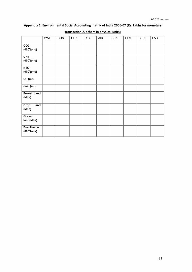
Appendix!1:!Environmental!Social!Accounting!matrix!of!India!2006?07!(Rs.!Lakhs!for!monetary!transaction!&!others!in!physical!units)!!

PAD WHT CER CAS ANH FRS FSH COL OIL PAD 3604537 56673 297765 333 45486 6 513 0 0 WHT 63062 2703447 377231 4 13612 0 6 0 0 CER 53742 128243 1813875 9 2555577 18 7 0 0 CAS 4048 14766 47603 798319 1295 0 0 0 0 ANH 586772 81354 954233 657037 26038 1 83 0 1 FRS 132 24 60 0 40 230 0 0 0 FSH 223 571 1182 0 0 0 246158 0 0 COL 47 35 74 15 202 0 0 11356 2 OIL 0 0 1 0 2590 0 0 0 54713 GAS 0 0 0 19 257 0 0 0 0 FBV 45025 6549 18793 14 272968 0 11467 0 0 TEX 21267 21413 15603 3338 2474 393 140281 88 3 WOD 81 209 433 43 236 11 6893 29899 3 MIN 1 3 9 1 503 0 0 0 16 PET 440637 197486 428076 200894 1292 3538 159517 42221 96751 CHM 3040 3257 5886 2217 19365 1043 9975 305214 68299 PAP 846 1023 1691 419 644 164 0 4436 3 FER 1551704 1351880 1533062 951908 194 44 219 0 0 CEM 0 0 0 0 33 1 0 0 857 IRS 0 1 7 1 1314 1 6856 2 1302 ALU 1 3 8 1 662 19 362 0 23 OMN 13173 8489 8675 4004 2950 3088 105725 109983 157816 MCH 63300 74441 81915 13137 6681 633 9 208316 193424 NHY 303163 292496 154790 47095 919 63 43 105965 28621 HYD 56174 54198 28682 8726 170 12 8 19635 5303 NUC 8532 8232 4356 1325 26 2 1 2982 806 BIO 62499 9197 108434 69230 13710 776 9 0 1 WAT 62 53 71 33 16 28 0 1859 0 CON 299358 186107 241647 95450 4927 3305 42 30402 299685 LTR 465228 308397 416869 214952 470359 10505 62115 145944 54946 RLY 218678 54027 77352 32208 28198 744 2773 8572 3718 AIR 33234 21421 15620 7991 2153 46 2312 697 1147 SEA 1017 1500 3189 362 32522 25 57 869 543 HLM 0 0 0 0 0 0 0 0 0 SER 848437 522990 860076 350991 2020029 9655 56472 179594 192200 Lab 3689555 2645224 13081859 4985874 7939400 155015 1870083 950571 880277 Cap 1115629 799304 3842846 1408910 7823192 166197 1535925 2387623 2272012 Land 2546449 1825601 9153113 3501862 RNASE RAL ROL RASE ROH USE USC UCL UOH PVT PUB GOV ITX -1139709 -1310720 -1108597 -581101 31009 11379 -202612 90587 81514 CAC ROW 53 31699 831853 283794 34943 626973 15046 1059286 14830033 TOT 14960001 10099591 33298342 13059415 21355984 993915 4030348 5696101 19224020

!

!

! 27!

Appendix!1:!Environmental!Social!Accounting!matrix!of!India!2006?07!(Rs.!Lakhs!for!monetary!

transaction!&!others!in!physical!units)!

PAD WHT CER CAS ANH FRS FSH COL OIL

CO2 (000'tons) 46959 30555 56342 73664 67800

CH4 (000'tons)

N2O (000'tons)

Oil (mt) 34

coal (mt) 361

Forest Land (Mha)

Crop land (Mha)

Grass land(Mha)

Env.Theme (000’tons)

!

!

!

!

!

!

!

!

!

!

!

!

!

!

!

!

Contd………..!

! 28!



GAS FBV TEX WOD MIN PET CHM PAP FER PAD 0 480042 41 8 3 0 20196 1773 340 WHT 0 915729 74 20 1 0 36804 137 735 CER 1 3051005 7501 503 81 880 308401 19754 4427 CAS 2 5426983 2056049 341 201 1637 728827 4493 8404 ANH 3 1601763 372582 325 153 308 157594 882 2331 FRS 4 19532 290 55073 37 217 16076 50715 69 FSH 0 458661 40 2 1 0 19972 172 356 COL 957 29140 27400 5525 23948 252434 139313 53150 32516 OIL 1376 194 12 300 58 18673034 211974 556 1 GAS 5 3010 36448 183 1484 886 327777 2027 381218 FBV 2 4300382 16609 498 218 1015 479422 11745 10967 TEX 19 106573 5501608 1518 3789 4247 368217 11427 9356 WOD 2114 170905 78689 14647 2562 9784 268310 67587 24950 MIN 70 4328 6850 1884 26313 2631 193568 4602 162315 PET 11260 406413 407654 7406 63514 1020947 1182041 84364 791718 CHM 28662 1241295 2158888 38087 121069 546658 15269445 421793 1275236 PAP 325 442279 160128 19331 1797 14496 962974 617782 8541 FER 3 61026 1978 6754 80 3612 225431 525 577350 CEM 53 76 370 140 218 3105 7641 70 55 IRS 329 1671 17261 8151 12877 4515 215983 13309 3104 ALU 116 3941 11634 3771 49536 10981 225889 7481 5077 OMN 19255 49225 196681 18950 64147 20287 564638 12863 9520 MCH 25725 275599 558968 7848 33712 41103 484615 15348 23692 NHY 15172 218487 616474 13510 61600 294141 789216 97953 79410 HYD 2811 40484 114228 2503 11414 54502 146236 18150 14714 NUC 427 6149 17350 380 1734 8278 22212 2757 2235 BIO 13 94233 1534 185645 130 781 59890 172836 313 WAT 133 6695 3641 46 404 209 11973 115 1729 CON 18053 333190 411837 2372 58265 192032 328759 9861 49682 LTR 17441 1665994 2120591 44524 45926 120362 1709841 195932 258956 RLY 1848 93918 29913 4081 14546 548377 166346 24430 40166 AIR 153 106956 7532 3512 1299 15347 31377 5648 13136 SEA 114 19230 37301 242 278 3792 52835 5044 1304 HLM 0 0 0 0 0 0 0 0 0 SER 27914 5985966 4626498 126727 171480 986547 4137078 325955 592151 Lab 422077 2468376 3448211 295948 832851 306368 3575263 259182 334750 Cap 423125 3621031 3414704 215792 2092439 4606321 7319453 423864 931988 Land RNASE RAL ROL RASE ROH USE USC UCL UOH PVT PUB GOV ITX 13229 768166 483529 20759 61959 1554145 2787084 233237 301979 CAC ROW 751027 2686079 1315523 78402 8023533 3604127 8735582 820494 548325 TOT 1783816 37164725 28266621 1185711 11783655 32908109 52288252 3998014 6503117

!

!

!

Contd………..!

! 29!



GAS FBV TEX WOD MIN PET CHM PAP FER

CO2 (000'tons)

CH4 (000'tons)

N2O (000'tons)

Oil (mt)

coal (mt)

Forest Land (Mha)

Crop land (Mha)

Grass land(Mha)


!

!

!

!

!

!

!

!

!

!

!

!

!

!

!

!

Contd………..!

! 30!



CEM IRS ALU OMN MCH NHY HYD NUC BIO PAD 0 19 1 1578 281 1309 0 0 5115 WHT 0 30 1 3020 546 2266 0 0 3042 CER 44 378 183 16627 3852 10779 0 0 213747 CAS 111 924 729 34391 9627 16922 0 0 2881 ANH 59 1459 1161 45847 12678 4697 0 0 6689 FRS 19 643 154 35230 2603 704 0 0 1832 FSH 0 17 1 1639 343 1226 0 0 223 COL 217084 2065513 457147 574505 114056 1692816 0 0 164 OIL 2 20936 1085 91313 4544 40917 0 0 209 GAS 35930 317837 26419 70721 35564 325683 0 0 27 FBV 166 2712 2049 22239 6140 12255 0 0 24024 TEX 9504 11516 4827 180233 196041 7383 0 0 3233 WOD 28946 16799 5632 171272 227330 2250 0 0 350 MIN 368646 651084 477031 1175277 213464 0 0 6146 54 PET 126628 734155 145332 863213 521420 1654974 0 0 28271 CHM 137084 308761 232203 2018159 2645906 117745 0 1711 10884 PAP 37859 20696 9488 186071 248553 27143 7055 497 3004 FER 17 5835 198 6348 6177 3234 0 0 6528 CEM 1419 4361 1758 72661 7136 31 24 0 9 IRS 3193 3560402 176752 3869196 6330835 18877 2020 0 147 ALU 1372 3380076 935163 2161226 4271787 18924 2551 0 212 OMN 171932 1036459 217809 7001479 4244945 361252 12119 5426 23057 MCH 7106 342501 157092 2824181 12649358 797475 40206 12174 5690 NHY 248364 1113522 190742 874539 603835 4222060 832 61371 1508 HYD 46020 206328 35343 162046 111887 782319 154 11372 280 NUC 6990 31339 5368 24613 16994 118826 23 1727 42 BIO 176 2237 555 119407 8788 2418 0 0 7717 WAT 23 633 187 20829 1912 21709 0 315 211 CON 9669 103161 68902 858778 1039096 353407 21809 5453 25876 LTR 127948 611392 161034 1316451 1293680 389306 11580 5827 118111 RLY 147032 955566 161873 524171 211815 531289 12148 7897 8184 AIR 13577 51495 11825 41876 12219 53022 406 776 635 SEA 655 3886 1032 32578 33574 4699 853 81 2670 HLM 0 0 0 0 0 0 0 0 0 SER 383060 3200680 651886 5679499 7705456 2107244 139633 32654 240078 Lab 251382 2243925 786206 5060576 3681199 320002 1087917 25610 1877973 Cap 624803 3903004 350669 7187010 4935561 2711260 1466763 241362 1859180 Land RNASE RAL ROL RASE ROH USE USC UCL UOH PVT PUB GOV ITX 111024 1029909 356922 2600023 4055593 -1769435 -32813 834 0 CAC ROW 629557 3333828 7439439 30835793 11813863 0 0 0 0 TOT 3747403 29274019 13074201 76764616 67278659 14966987 2773280 421233 4481857

!

!

!

Contd………..!

! 31!



!

CEM IRS ALU OMN MCH NHY HYD NUC BIO

CO2 (000'tons)

CH4 (000'tons)

N2O (000'tons)

Oil (mt)

coal (mt)

Forest Land (Mha)

Crop land (Mha)

Grass land(Mha)


!

!

!

!

!

!

!

!

!

!

!

!

!

!

!

!

Contd………..!

! 32!



WAT CON LTR RLY AIR SEA HLM SER Lab PAD 49 113 18 0 0 111 3612 718905 WHT 93 80 1300 0 0 117 4530 397700 CER 388 1061416 953328 0 0 712 13580 2341984 CAS 611 800 0 0 2 0 0 146536 ANH 178 601652 0 0 0 0 10338 1285048 FRS 41 83419 0 9 0 0 0 2992 FSH 50 43 0 0 0 0 0 17098 COL 101 1970 0 4164 0 0 0 20790 OIL 619 23 0 0 11 0 0 13295 GAS 163 325 0 0 0 0 0 6777 FBV 543 424 18874 0 0 837 0 2467947 TEX 112 93123 79766 910 50 941 17421 152856 WOD 99 919489 1068 97 0 0 0 23867 MIN 10 3729164 0 0 0 0 0 27148 PET 2190 3355210 12200344 268248 97767 43643 70748 950541 CHM 6332 1141838 2324087 8258 135793 183592 2391228 1138535 PAP 1524 36405 153476 4697 951 460 14464 287397 FER 1241 11379 230 6 0 0 0 14203 CEM 0 3969131 0 0 0 0 0 1738 IRS 2159 10273278 891 409 0 0 0 207244 ALU 57 3853 326 0 0 0 0 122373 OMN 4979 8386495 2113947 1250215 91698 103333 133745 2538691 MCH 4336 2366624 933154 41763 5363 12665 104722 2176907 NHY 22460 895618 28247 695572 2400 5157 15150 647088 HYD 4162 165952 5234 128885 445 956 2807 119901 NUC 632 25206 795 19576 68 145 426 18212 BIO 140 285604 4041 29 0 3 58 20010 WAT 141549 177244 15485 320 985 18334 900 109167 CON 116775 3790532 642021 866250 36259 36649 222340 3491684 LTR 6722 4110131 2382395 91440 60647 77416 227590 3952304 RLY 656 981304 532260 568506 1416 1228 1859 114131 AIR 47 92231 142044 3437 1177 512 1043 57923 SEA 183 25850 41715 1673 375 201 43820 103162 HLM 0 0 0 100676 0 0 0 173246 SER 89571 9607585 8210058 232405 112249 176900 761775 19477882 Lab 326430 22499481 9807816 2462740 263300 578908 4692207 71922015 Cap 363570 9461837 7531709 1774196 197957 415166 2693040 95799645 Land RNASE 13686272 RAL 30655386 ROL 9597032 RASE 23604200 ROH 6014659 USE 17416862 USC 63190125 UCL 9330416 UOH 2282323 PVT PUB GOV ITX 8260 2468171 2627536 224044 44498 48704 414210 790126 CAC ROW 0 0 478851 0 0 0 0 7888498 TOT 1107034 90622999 51231016 8748525 1053410 1706690 11841614 219745567 175777274

!

!

!

Contd………..!

! 33!



WAT CON LTR RLY AIR SEA HLM SER LAB

CO2 (000'tons)

CH4 (000'tons)

N2O (000'tons)

Oil (mt)

coal (mt)

Forest Land (Mha)

Crop land (Mha)

Grass land(Mha)


!

!

!

!

!

!

!

!

!

!

!

!

!

!

!

!

Contd………..!

! 34!



Cap Land RNASE RAL ROL RASE ROH USE USC PAD 921172 1929082 465192 2615038 686698 882091 971107 WHT 527070 1103765 266169 1496249 392909 504706 555640 CER 1827586 3590841 947921 4944834 1532174 2474139 2817419 CAS 299626 627464 151311 850582 223359 286913 315868 ANH 1203885 1541555 566288 4038074 1205631 2093656 2433331 FRS 56650 106912 28156 168129 46044 38522 42409 FSH 270564 566605 136635 768082 201695 259085 285231 COL 2587 4806 1392 7050 2297 3982 4539 OIL 0 0 0 0 0 0 0 GAS 8530 15845 4591 23244 7574 13128 14966 FBV 2337903 4286378 1252981 6672925 2092675 3174404 3775280 TEX 1086663 1857987 535414 3279454 1057461 1576595 1917142 WOD 5587 5428 2970 18109 5942 11599 15773 MIN 0 0 0 0 0 0 0 PET 345403 571748 238310 1112680 650630 723282 1928089 CHM 419787 578193 220158 1431805 465963 850403 1564865 PAP 27994 36969 13736 96565 26651 56321 93756 FER 0 0 0 0 0 0 0 CEM 0 0 0 0 0 0 0 IRS 0 0 0 0 0 0 0 ALU 0 0 0 0 0 0 0 OMN 330690 364709 172486 1016206 356694 699474 968900 MCH 386716 426498 201709 1188372 417126 817979 1133052 NHY 149390 277486 80407 407068 132646 229909 262088 HYD 27681 51416 14899 75427 24578 42600 48563 NUC 4204 7810 2263 11457 3733 6471 7376 BIO 363625 686243 180725 1079176 295545 247261 272214 WAT 9931 18447 5345 27062 8818 15284 17423 CON 170198 280178 90104 537936 181655 295588 465387 LTR 1616071 2134167 792934 5560509 1538523 3251313 5412380 RLY 77718 102633 38133 288570 73988 156357 260284 AIR 18739 24745 9194 -48923 17839 37698 62755 SEA 58125 76759 28519 307632 55336 116939 194666 HLM 534718 1300190 354222 2104424 1185892 930716 1834783 SER 4613267 6644682 2597189 15922245 6145036 10965155 21129082 Lab Cap Land RNASE 11301847 RAL 99289 ROL 591941 RASE 28570049 17027026 ROH 17120543 USE 19042479 USC 4147757 UCL 1346862 UOH 6309825 PVT 32937007 PUB 9545700 GOV 7439300 355411 0 0 4142314 1419397 0 2379634 ITX 802814 1317718 426876 2548941 867247 1406262 2238702 CAC 44737987 10554871 5666113 2167887 18770185 5912228 10750880 25845192 ROW TOT 183190587 17027026 29415175 36203372 11994117 81461420 27233983 42918713 79267896

!

!

!

Contd………..!

! 35!



CAP LAND RNASE RAL ROL RASE ROH USE USC

CO2 (000'tons)

CH4 (000'tons)

N2O (000'tons)

Oil (mt)

coal (mt)

Forest Land (Mha) 0.16

Crop land (Mha) 0.45

Grass land(Mha) 0.01

Env.Theme (000’tons) 1769746

!

!

!

!

!

!

!

!

!

!

!

!

!

!

!

!

Contd………..!

! 36!



UCL UOH PVT PUB GOV ITX CAC ROW TOT PAD 295510 156272 102487 101482 595043 14960001 WHT 169082 89414 53035 -115959 533924 10099591 CER 662037 460271 185878 551811 742389 33298342 CAS 96119 50830 0 709321 141521 13059415 ANH 405042 396006 340150 438181 282915 21355984 FRS 12905 6825 61 4938 212218 993915 FSH 86796 45899 0 4929 656848 4030348 COL 1797 815 6326 -80482 16566 5696101 OIL 0 0 0 -6482 112740 19224020 GAS 5924 2688 27381 11623 75561 1783816 FBV 892075 647357 398033 1400206 2500625 37164725 TEX 342432 326420 328519 594522 8394477 28266621 WOD 1513 2298 107 -1003963 45794 1185711 MIN 0 0 0 -130444 4862982 11783655 PET 211808 209213 421402 -2900636 2787765 32908109 CHM 188901 230639 908608 4992972 6114416 52288252 PAP 11664 15059 80533 94443 167706 3998014 FER 0 0 213 -58531 240268 6503117 CEM 0 0 0 -330620 7135 3747403 IRS 0 0 0 1842627 2699301 29274019 ALU 0 0 0 543543 1313233 13074201 OMN 100834 150272 539350 21869319 21128635 76764616 MCH 117917 175731 580572 30745595 6497608 67278659 NHY 103738 47068 529604 0 0 14966987 HYD 19222 8721 98132 0 0 2773280 NUC 2920 1325 14905 0 0 421233 BIO 82835 43821 0 0 0 4481857 WAT 6896 3129 457828 0 0 1107034 CON 69489 84079 738347 73456402 0 90622999 LTR 673354 869322 844476 1440554 3824555 51231016 RLY 32382 41806 151856 455432 958135 8748525 AIR 7807 10080 20100 33413 106138 1053410 SEA 24218 31267 45962 197583 112451 1706690 HLM 322525 810765 2189457 0 0 11841614 SER 2307761 3926428 33042548 4512415 27110384 219745567 Lab -251300 175777274 Cap -2726500 183190587 Land 17027026 RNASE 3307145 1119912 29415175 RAL 4070341 1378356 36203372 ROL 1348497 456647 11994117 RASE 9158699 3101446 81461420 ROH 3061914 1036868 27233983 USE 4825346 1634026 42918713 USC 8912081 3017933 79267896 UCL 1413124 478532 12568935 UOH 1137160 385081 10114388 PVT 2163093 35100100 PUB 9545700 GOV 3975924 634321 14434600 35574693 4669800 75025393 ITX 330440.287 408564 594826 8762980 795880 35574693 CAC 1007065 227683 20665500 9545700 -7072703 -641415 148137174 ROW 106696599 TOT 12568935 10114388 35100100 9545700 75025393 35574693 148137174 106696599

!

!

Contd………..!

! 37!



UCL UOH PVT PUB GOV ITX CAC ROW TOT

CO2 (000'tons)

CH4 (000'tons)

N2O (000'tons)

Oil (mt)

coal (mt)

Forest Land (Mha)

Crop land (Mha)

Grass land(Mha)


!

!

!

!

!

!

!

!

!

!

!

!

!

!

!

!

Contd………..!

! 38!



CO2 000'tons)

CH4 (000'tons)

N2O (000'tons)

Oil (mt) coal (mt)

Forest Land (Mha)

Crop land (Mha)

Grass and(Mha)

Env.Theme (000'tons)

PAD 11589 3327 41 94028 WHT 8477 0 35 19420 CER 18240 0 40 30705 CAS 3615 0 25 11305 ANH 49426 10216 1 264278 FRS 0 0 0 0 FSH 1 0 0 1 COL 730 8410 15330 OIL 71 20 1495 GAS 708 14872 FBV 27626 7 0 27837 TEX 1861 26 0 2413 WOD 351 0 0 353 MIN 1460 0 0 1465 PET 33788 4 0 33886 CHM 27889 14 17 33555 PAP 5223 25 0 5780 FER 31514 3 1 31765 CEM 129920 129920 IRS 116958 15 1 117621 ALU 2729 0 0 2729 OMN 41822 1 1 42092 MCH 17662 0 0 17776 NHY 715830 980 11 739704 HYD 0 NUC 0 BIO 0 WAT 0 CON 89 0 0 90 LTR 121211 23 6 123554 RLY 6109 0 2 6845 AIR 10122 0 0 10211 SEA 1416 0 0 1431 HLM 0 SER 1568 0 0 1583 Lab 0 Cap 0 Land 0.09 1.34 0.20 0 RNASE 16306 190.189 3 21215.69 21216 RAL 29861 323 5 38226.28 38226 ROL 8866 124 2 12056.42 12056 RASE 49358 602 9 64877.3 64877 ROH 17461 320 5 25597.61 25598 USE 8403 919 4 29074.43 29074 USC 22105 1454 12 56212.31 56212 UCL 2492 284 1 8858.502 8858 UOH 2414 197 1 6943.122 6943 PVT PUB GOV ITX CAC ROW TOT

!

!

Contd………..!

! 39!



CO2 (000'tons)

CH4 (000'tons)

N2O (000'tons)

Oil (mt)

coal (mt)

Forest Land (Mha)

Crop land (Mha)

Grass land(Mha)

Env.theme (000' tons)

CO2 (000'tons) -275358

CH4 (000'tons)

N2O (000'tons)

Oil (mt)

Coal (mt)

Forest Land (Mha)

Crop land (Mha)

Grass land(Mha) 10490


Contd………..!

identifying key sectors for green growth in india: an

Documents