Atmos. Chem. Phys., 21, 15631–15646, 2021https://doi.org/10.5194/acp-21-15631-2021© Author(s) 2021. This work is distributed underthe Creative Commons Attribution 4.0 License.

Identifying the spatiotemporal variations in ozone formationregimes across China from 2005 to 2019 based on polynomialsimulation and causality analysisRuiyuan Li1, Miaoqing Xu1, Manchun Li2, Ziyue Chen1, Na Zhao3,4, Bingbo Gao5, and Qi Yao1

1State Key Laboratory of Remote Sensing Science, College of Global Change and Earth System Sciences,Beijing Normal University, Beijing, 100875, China2School of Geography and Ocean Science, Nanjing University, Nanjing, 210023, China3State Key Laboratory of Resources and Environment Information System, Institute of Geographic Sciences and NaturalResources Research, Chinese Academy of Sciences, Beijing, 100049, China4University of Chinese Academy of Sciences, Beijing, 100080, China5College of Land Science and Technology, China Agriculture University, Beijing, 100083, China

Correspondence: Ziyue Chen (zychen@bnu.edu.cn)

Received: 5 April 2021 – Discussion started: 30 April 2021Revised: 11 August 2021 – Accepted: 1 September 2021 – Published: 19 October 2021

Abstract. Ozone formation regimes are closely related tothe ratio of volatile organic compounds (VOCs) to NOx .Different ranges of HCHO/NO2 indicate three formationregimes, including VOC-limited, transitional, and NOx-limited regimes. Due to the unstable interactions between adiversity of precursors, the range of the transitional regime,which plays a key role in identifying ozone formationregimes, remains unclear. To overcome the uncertaintiesfrom single models and the lack of reference data, we em-ployed two models, polynomial simulation and convergentcross-mapping (CCM), to identify the ranges of HCHO/NO2across China based on ground observations and remote sens-ing datasets. The ranges of the transitional regime estimatedby polynomial simulation and CCM were [1.0, 1.9] and [1.0,1.8]. Since 2013, the ozone formation regime has changed tothe transitional and NOx-limited regime all over China, indi-cating that ozone concentrations across China were mainlycontrolled by NOx . However, despite the NO2 concentra-tions, HCHO concentrations continuously exert a positive in-fluence on ozone concentrations under transitional and NOx-limited regimes. Under the circumstance of national NOxreduction policies, the increase in VOCs became the majordriver for the soaring ozone pollution across China. For aneffective management of ozone pollution across China, the

emission reduction in VOCs and NOx should be equally con-sidered.

1 Introduction

With the significant improvement of PM2.5 pollution, sur-face ozone has become a major airborne pollutant acrossChina since 2017 (Li et al., 2019a; Lu et al., 2020). Due toits severe threat to public health even during a short-periodexposure, ozone pollution has received growing emphasisfrom governments and scholars (H. Liu et al., 2018; Xie etal., 2019). In the past several years, spatiotemporal distribu-tion of ozone concentrations (Wu and Xie, 2017; Shen etal., 2019a) and the influence of meteorological conditions(Chen et al., 2019c; Cheng et al., 2019, 2020) and anthro-pogenic emissions (Chen et al., 2019b; Cheng et al., 2018; Liet al., 2019a, 2020) on ozone concentrations have been mas-sively studied. However, due to the highly complicated ozoneformation regime, effective ozone control remains challeng-ing.

Different from PM2.5, whose main precursors are NOx ,volatile organic compounds (VOCs), and SO2, the forma-tion and decomposition of ozone are closely related to twotypes of precursors, VOCs and NOx . There is a diversity of

Published by Copernicus Publications on behalf of the European Geosciences Union.

15632 R. Li et al.: Identifying the spatiotemporal variations in ozone formation regimes across China

reactions between VOCs and NOx under different meteoro-logical conditions and concentration scenarios (Wang et al.,2017). Since VOCs and NOx can either promote or restrictozone production, the VOCs/NOx ratio is crucial for sur-face ozone concentrations. However, the thresholds at whichVOCs/NOx may promote or restrict ozone production re-main unclear (Jin et al., 2017; Schroeder et al., 2017). Forinstance, under a specific VOCs/NOx scenario, the reduc-tion in NOx may conversely increase surface ozone concen-trations (Sillman et al., 1990; Kleinman, 1994). Furthermore,given the large variations in meteorological conditions andthe ozone level across China, the effects of VOCs/NOx onsurface ozone concentrations also demonstrate notable spa-tiotemporal patterns. In this case, a comprehensive under-standing of how the variations in VOCs and NOx could in-fluence ozone concentrations under different VOCs/NOx cir-cumstances is crucial for setting effective emission reductionpolicies accordingly in different regions.

To examine the complicated nonlinear relationship be-tween ozone concentrations and multiple precursors, a largebody of studies has been conducted (Duncan et al., 2010;Choi et al., 2012; Pusede and Cohen, 2012; Chang etal., 2016; Jin et al., 2020). Through small-scale experiments,NO2 and HCHO proved to be effective proxies for NOx andVOCs (Sillman et al., 1990; Martin et al., 2004). Since NO2and HCHO can be monitored using remote sensing data, thetwo precursors have been increasingly considered in ozone–precursor sensitivity research (Jin et al., 2020; X. Zhang etal., 2020). Cheng et al. (2018) proved that NO2/NO pre-sented a good consistence with long-term ozone concentra-tions in Beijing. However, NO was not an easily recordableprecursor based on satellite observations and not applica-ble in large-scale monitoring. Cheng et al. (2019) suggestedthat satellite-retrieved HCHO/NO2 was strongly correlatedwith surface ozone concentrations in Beijing. DifferentHCHO/NO2 indicates distinct ozone formation regimes, in-cluding VOC-limited, transitional, and NOx-limited regimes.For the VOC-limited (NOx-saturated) regime, the controlof VOC emissions leads to the reduction in organic radi-cals (RO2), the RO2–NOx reactions and thus ozone concen-trations (Milford et al., 1989). In contrast, the decrease inNOx promotes VOC–CO reaction, leading to the increase inozone concentration (Kleinman, 1994). For the NOx-limitedregime, the reduction in NOx slows down NO2 photolysis,which produces free oxygen atoms for ozone formation andreduces ozone concentrations. The variations in VOCs exertlimited influences on ozone concentrations for this regime(Kleinman, 1994). For the transitional (VOC–NOx mixed)regime, both VOCs and NOx impose positive influences onozone concentrations. Since the transitional regime dividesVOC-limited and NOx-limited regimes, the estimation of thetransitional regime range plays a key role in identifying dif-ferent ozone formation regimes.

Duncan et al. (2010) calculated the transitional regimerange as [1.0, 2.0] using the Community Multiscale Air

Quality Modeling System (CMAQ) model, whose uncertain-ties may influence the estimation accuracy (Schroeder et al.,2017). Jin et al. (2020) employed a polynomial model andcalculated the transitional regime range over US urban ar-eas as [3.2, 4.1] based on decades of remote sensing andground observation data. However, given the notable dif-ference in meteorological conditions, ozone levels, and thecomposition of precursors across different countries, whetherthe transitional regime range extracted in the US is appli-cable to other countries remains unclear. Furthermore, thepolynomial model may ignore the complicated inner inter-actions between multiple precursors, meteorological factors,and ozone concentrations in the atmospheric environment(Chen et al., 2020) and may lead to large uncertainties. Con-sequently, ozone–precursor sensitivity, especially the transi-tional regime range across China, requires further in-depthanalysis.

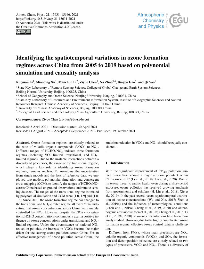
To this end, this research attempts to investigate the spa-tiotemporal variations in ozone formation regimes acrossChina and identify the transitional regime range ofHCHO/NO2 based on the cross-verification of multiplemodels. Firstly, long-term variations in HCHO and NO2across China were analyzed. Next, the datasets of HCHO,NO2, and ozone were examined using a polynomial modeland a causality model, respectively, to reveal the crucialthresholds of HCHO/NO2 that separate the NOx-limited,VOC-limited, and transitional regimes. Specifically, due tothe large area of China and potential spatial variations inozone formation regimes, we respectively investigated ozoneformation regimes in several major regions, including theNorth China Plain (NCP), Yangtze River Delta (YRD), PearlRiver Delta (PRD), and Sichuan Basin (SCB) (the geographi-cal locations of four megacity clusters were shown in Fig. 1),to explore the spatiotemporal variations in ozone formationregimes. Meanwhile, we also compared the ozone formationregimes in urban and rural areas. This research sheds usefullight for better modeling the complicated ozone–precursorrelationship, understanding the major drivers for enhancedozone pollution, and implementing specific emission reduc-tion measures to mitigate ozone pollution across China.

2 Materials and methods

2.1 Data sources

In this study, Ozone Monitoring Instrument (OMI)HCHO/NO2 datasets were employed for exploring thespatiotemporal variations in HCHO and NO2 in Chinaand calculating HCHO/NO2. We connected surface ozonenetwork data to HCHO, NO2, and HCHO/NO2, whichserved as the input data for running third-polynomial modeland convergent cross-mapping (CCM). The MODIS landcover product provided the spatial distribution of urban

Atmos. Chem. Phys., 21, 15631–15646, 2021 https://doi.org/10.5194/acp-21-15631-2021

R. Li et al.: Identifying the spatiotemporal variations in ozone formation regimes across China 15633

Figure 1. The May-to-September mean hourly surface ozone net-work data from 2014 to 2019. Mean hourly surface ozone con-centrations are calculated on the 0.25◦× 0.25◦ grid. Purple, blue,green, and red outlines indicate the boundaries of North China Plain(NCP), Yangtze River Delta (YRD), Pearl River Delta (PRD), andSichuan Basin (SCB), respectively.

areas, which was employed for identifying urban and ruralpixels.

2.1.1 OMI HCHO/NO2

The Ozone Monitoring Instrument (OMI), on board the Aurasatellite, monitors global solar backscatter in the UV–visdomain (270–500 nm). The OMI provides daily global ob-servations and crosses the Equator at 13:38 LT (Levelt etal., 2006). In this study, we employed the daily level-3 grid-ded OMI HCHO product (OMHCHOd) from the Smith As-trophysical Observatory (SAO) (González Abad et al., 2015).The HCHO vertical columns are the weighted mean valuesfor the 0.1◦× 0.1◦ grid. Backscattered solar radiation, rang-ing from 328.5–356.5 nm, was used for fitting HCHO slantcolumns. Air mass factors (AMFs) were employed for con-verting HCHO slant columns to vertical columns (GonzálezAbad et al., 2015). The validation report suggested that theerror in this product was effectively controlled within 30 %over polluted areas (González Abad et al., 2015) and vali-dated for detecting long-term variations in HCHO columns(Zhu et al., 2017; Shen et al., 2019b). The daily level-3 grid-ded OMI NO2 product (OMNO2d), provided by NASA’sGoddard Space Flight Center, was utilized in this study (Buc-sela et al., 2013; Lamsal et al., 2014). The spatial resolu-tion of OMNO2d is 0.25◦, and each grid is generated as theweighted average of the corresponding level-2 data pixels(Krotkov et al., 2017). Differential optical absorption spec-troscopy (DOAS) was employed for retrieving the NO2 slantcolumns, which were successively transformed into tropo-spheric and stratospheric vertical columns through AMFs

(Bucsela et al., 2013). The OMI NO2 column product agreeswell with other satellite products, and its overall uncertain-ties range from 30 %–60 % (Bucsela et al., 2013; Lamsal etal., 2014). To reduce uncertainties, we only selected thoseOMI HCHO and NO2 data that (1) passed quality checks,(2) had a cloud coverage less than 30 %, (3) had a solarzenith angle less than 60◦, and (4) were not affected byrow anomalies for this study (Kroon et al., 2011; Zhu etal., 2014; Krotkov et al., 2017). The May-to-September OMIHCHO and NO2 products were acquired from NASA’s God-dard Earth Sciences Data and Information Services Center(https://disc.gsfc.nasa.gov/, last access: 1 September 2021).

2.1.2 Surface ozone network data

The May-to-September hourly surface ozone concentrationsfrom 2014 to 2019 were obtained from the China Ministry ofEcology and Environment (MEE) (https://quotsoft.net/air/,last access: 1 September 2021). The unit of surface ozoneconcentrations in this dataset is µgm−3. The network had1633 monitoring stations, which were distributed among 330cities across China in 2019. We used the observation datafrom 13:00 to 14:00 LT to match the overpass time of theOMI. This dataset has been employed in many studies toinvestigate the variations in surface ozone concentrations inChina (Li et al., 2019a; Shen et al., 2019a; Lu et al., 2020).

2.1.3 MODIS land cover product

The annual MODIS land cover product (MCD12C1) with aspatial resolution of 0.05◦ from 2005 to 2019 was employedfor extracting urban and rural areas. The urban and waterpixels from the International Geosphere–Biosphere Program(IGBP) classification layer were employed for the followingprocessing. The land cover product was generated based ona decision tree algorithm with boosting techniques, and itsoverall accuracy was about 75 % (Palmer et al., 2015; Ba-jocco et al., 2018). The MCD12C1 product was obtainedfrom NASA’s Earth System Data and Information System(https://earthdata.nasa.gov/, last access: 1 September 2021).

2.1.4 Data pre-processing

Due to the different spatial resolution of OMI HCHO, OMINO2, and MCD12C1, a bilinear interpolation method wasused for resampling all abovementioned products to thesame spatial size (0.25◦× 0.25◦). Meanwhile, we also cal-culated mean hourly surface ozone concentrations on the0.25◦× 0.25◦ grid (Fig. 1).

2.2 Methods

Chemical transport models, such as the global chemicaltransport model (GEOS-Chem) (Jin et al., 2017; Li etal., 2019a) and the Community Multiscale Air Quality Mod-eling System (CMAQ) (Duncan et al., 2010), have been

https://doi.org/10.5194/acp-21-15631-2021 Atmos. Chem. Phys., 21, 15631–15646, 2021

15634 R. Li et al.: Identifying the spatiotemporal variations in ozone formation regimes across China

frequently employed for exploring the ozone sensitivity toVOCs and NOx . However, there were large biases in esti-mating the range of the transitional regime based on chemi-cal transport models (Jin et al., 2017, 2020) due to the uncer-tainties in the emission inventory and the setting of model pa-rameters. Employing observation data alone could effectivelyovercome these limitations, and the relationships betweenozone and its precursors were fitted using linear and polyno-mial models (Sun et al., 2018; Jin et al., 2020). Meanwhile,convergent cross-mapping (CCM) (Sugihara et al., 2012), asa robust causality analysis model, has been widely employedfor quantifying the influences of meteorological factors onsurface ozone and PM2.5 concentrations (Chen et al., 2018,2019c, 2020). It is a promising tool for investigating the re-lationships between ozone and its precursors. To increase thereliability of the estimated range of the transitional regime,both the polynomial model and CCM were employed in thisresearch. We employed the third-order polynomial modelfor fitting surface ozone concentrations to the indicator ofHCHO/NO2. CCM was employed for quantifying the influ-ences of HCHO and NO2 on surface ozone concentrations,and the Wilcoxon test (Gehan, 1965) was used for examiningwhether the differences between the causality of HCHO onozone and NO2 on ozone at different ranges of HCHO/NO2was significant. Since the algorithms of the two models arequite different, their cross-verification provides useful refer-ence for their reliability. Meanwhile, the Mann–Kendall (M–K) test (Kendall, 1970) was employed for exploring the spa-tiotemporal variations in HCHO, NO2, and ozone formationregimes in China. Furthermore, we extracted all urban andrural areas in China and compared the differences in ozoneformation regimes over these two types of areas. The work-flow of the models employed in this study is shown in Fig. 2.

2.2.1 Estimating the transitional range of the ozoneformation regime using polynomial simulation

HCHO and NO2 are considered to be proxies for VOCs andNOx , respectively. HCHO/NO2, as an effective indicator,has been widely employed for determining ozone formationregimes (Duncan et al., 2010; Jin and Holloway, 2015; Jinet al., 2017, 2020; Cheng et al., 2019). Pusede and Cohen(2012) suggested that ozone exceedance probability (OEP)was an effective indicator to interpret the ozone sensitiv-ity to its precursors. The indicator is defined as the propor-tion of non-attainment events (surface ozone concentrationsexceeding 200 µgm−3) in total events at a given range ofHCHO/NO2:

OEP=Eventsnon-attainment

Eventsattainment+Eventsnon-attainment, (1)

where Eventsattainment and Eventsnon-attainment denote the at-tainment and non-attainment events, respectively (Pusedeand Cohen, 2012; Jin et al., 2020).

In this study, we used a third-order polynomial model (Jinet al., 2020) to explore the quantitative relationships betweenHCHO/NO2 and ozone exceedance probability. There were174 868 paired observations of surface ozone concentrationsand HCHO/NO2 from 2014 to 2019. The peak of fittingcurve highlights the turning point of VOC-limited and NOx-limited regimes (Jin et al., 2020). The range of HCHO/NO2,which corresponded to the top 10 % ozone exceedance prob-ability, was defined as the transitional regime. Since weaimed to apply a global model to determine the transitionalrange, it was necessary to examine whether the surface ozoneconcentrations in China were of spatially stratified hetero-geneity (SSH), as suggested by Wang et al. (2016). We em-ployed the geographical detector (Wang et al., 2010) to mea-sure the SSH of surface ozone concentrations. The geograph-ical detector calculates the q statistic to quantify SSH, andthe equation is summarized as follows:

q = 1−∑Lh=1Nhσ

2h

Nσ 2 , (2)

where N and σ 2 denote the number of samples and the vari-ance of population, and h is the number of stratifications.The range of the q statistic is [0, 1]. The larger the q statisticis, the stronger the SSH is. In this study, the boundaries offour megacity clusters served as strata. If the SSH is detectedbased on the abovementioned stratification, we could applythe polynomial model in each strata separately.

2.2.2 Estimating the transitional range of the ozoneformation regime using convergentcross-mapping

We also employed a causality model named convergentcross-mapping (CCM) (Sugihara et al., 2012), which couldreduce the influences of other factors such as meteorologicalconditions (Chen et al., 2019c, 2020), to extract the causalinfluences of HCHO and NO2 on surface ozone concentra-tions. Thanks to its capability of detecting weak coupling,CCM is advantageous for reliably comparing the influencesof different meteorological factors on surface ozone concen-trations (Chen et al., 2020). Therefore, we employed CCMto compare the sensitivity of ozone to HCHO and NO2 atdifferent ranges of HCHO/NO2. CCM utilizes convergentmaps to demonstrate the bidirectional coupling between thetime series of two variables. A convergent curve indicatesthat one variable imposes influences on the other variable,whilst a non-convergent curve denotes no causality betweentwo variables. The main idea of CCM is summarized as fol-lows. Firstly, CCM defines {X} and {Y } as the temporal vari-ations in two variables X and Y . {X} generates the shadowmanifold MX. Following this, the location of the lagged-coordinate vector onMX, x(t) is determined, and then E+1nearest neighboring points of x(t) are extracted. Finally, thecross-mapped estimate of Y (t), Y (t)|MX is calculated as fol-

Atmos. Chem. Phys., 21, 15631–15646, 2021 https://doi.org/10.5194/acp-21-15631-2021

R. Li et al.: Identifying the spatiotemporal variations in ozone formation regimes across China 15635

Figure 2. The workflow of the polynomial simulation and the causality analysis.

lows:

Y (t)|MX =

E+1∑i=1

ωiY (ti), (3)

where ωi stands for a weight calculated based on the dis-tance between X(t) and its ith nearest neighboring point.Y (ti) stands for the contemporaneous value of Y . CCM cal-culates cross-map skill (ρ value), which explains the quan-titative relationships. Number of dimensions for the attrac-tor reconstruction (E), time lag (τ ), and number of near-est neighbors to use for prediction (b) are required param-eters for CCM. According to previous studies (Chen et al.,2019c, 2020), E, τ , and b were set as 3, 2, and 4, respec-tively. Since the existence of missing values imposes nega-tive impacts on CCM results, only the consecutive time serieswere retained for this research. There were 1660 observationrecords of HCHO time series, NO2 time series, and corre-

sponding surface ozone time series. CCM was implementedusing the “pyEDM” package in Python. The Wilcoxon test(Gehan, 1965) was used to examine whether the differencesin ρ values between HCHO and NO2 were significant at thegiven HCHO/NO2. No significant difference was regardedas the transitional regime, while significant difference indi-cated the VOC-limited or NOx-limited regime.

2.2.3 Trend analysis

The Mann–Kendall (M–K) (Kendall, 1970) test, which hasbeen used in recent studies on HCHO and NO2 (Cheng etal., 2019; Wang et al., 2019; Zeb et al., 2019), was employedto estimate the significance of trends. The M–K test is ca-pable of processing samples with random distributions andmitigating the effects of outliers. The Z value is calculated

https://doi.org/10.5194/acp-21-15631-2021 Atmos. Chem. Phys., 21, 15631–15646, 2021

15636 R. Li et al.: Identifying the spatiotemporal variations in ozone formation regimes across China

Figure 3. The geographical locations of urban area, urban fringe,and rural area.

as follows:

Z =

[S−1√

Var(S)(S > 0)

S+1√

Var(S)(S < 0)

], (4)

where S denotes the statistic to be tested, and Var(S) standsfor the variance of S. The sign and absolute value of Z in-dicate the direction and significance of trends, respectively.Specifically, the positive and negative values of Z indicatethe upward and downward trend; 1.28, 1.64, and 2.32 are thethreshold values of |Z|, indicating that the trends of samplespass the tests at 90 %, 95 %, and 99 %, respectively.

2.2.4 Comparison of ozone formation regimes in urbanand rural areas in China

To compare the differences in ozone formation regimes inurban and rural areas in China, the key step is to extract ur-ban and rural pixels, respectively. Urban pixels were used forbuffer analysis (Imhoff et al., 2010) to identify rural pixels.Following Peng et al. (2018), two buffers were set for ur-ban pixels to extract candidate rural pixels (Fig. 3). We setthe size of each buffer as 27.75 km, which was close to thesize of the 0.25◦× 0.25◦ grid (27.75km≈ 0.25◦). The firstand second buffers were determined as the urban fringes andcandidate rural areas, respectively. Water pixels were firstlyremoved from candidate rural areas to avoid following uncer-tainties. Consequently, rural areas were regarded as buffersof 27.75–55.50 km surrounding urban areas. The use of twobuffers not only assisted a complete separation of the urbanand rural areas but also minimized the uncertainties in mete-orological conditions (Yao et al., 2019).

3 Results

3.1 Spatial and temporal variations in HCHO and NO2

Given the national Clean Air Action implemented in 2013,we set this year as a break point to explore the spatial andtemporal variations in HCHO and NO2 in 2005–2012 and2013–2019, respectively. Figure 4 shows the spatial distri-bution of HCHO in the two periods. The mean HCHO val-ues during the period of 2005–2012 and 2013–2019 were4.335×1015 and 4.845×1015 molec.cm−2, characterized by

a 12 % increase. Both periods presented an increasing trendof HCHO, and the averaged values during the two peri-ods were 0.164× 1015 and 0.213× 1015 molec.cm−2 yr−1

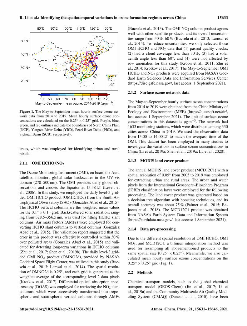
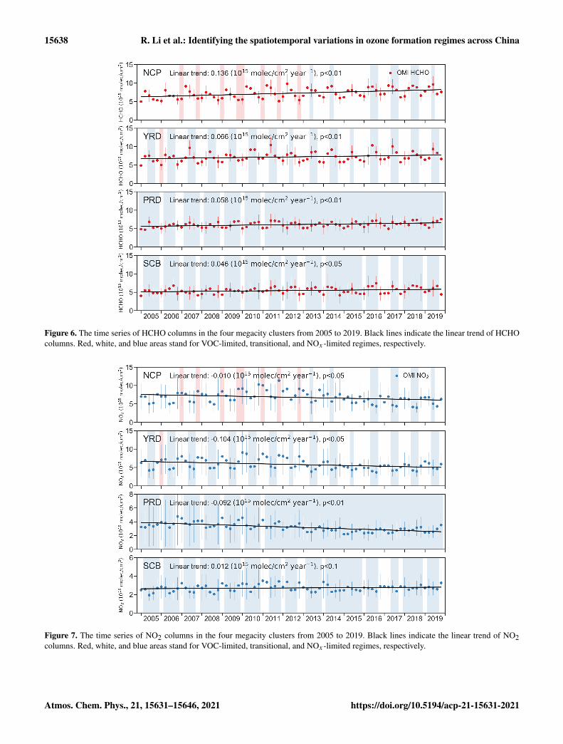
(Fig. 5). A faster increasing trend was detected during theperiod of 2013–2019. The variation trend of HCHO agreedwell with previous studies (Jin and Holloway, 2015; Shen etal., 2019b). We also calculated the overall linear trends ofHCHO in four megacity clusters from 2005 to 2019 (Fig. 6).The largest and smallest increasing trends were shown inthe NCP and SCB, with a mean value of 0.136× 1015 and0.046× 1015 molec.cm−2 yr−1. The increasing trends of theYRD and PRD were 0.066 and 0.058 molec.cm−2 yr−1, re-spectively. Meanwhile, reversed trends were detected forNO2 during the two periods (Fig. 5), which was consis-tent with previous studies (Jin and Holloway, 2015; Li etal., 2019a). From 2005 to 2012, the averaged NO2 was2.027× 1015 molec.cm−2, and the annual mean increasingtrend was 0.098× 1015 molec.cm−2 yr−1. Thanks to the im-plementation of the Clean Air Action, the averaged NO2 wasreduced to 1.900×1015 molec.cm−2, with a decreasing trendof −0.029× 1015 molec.cm−2 yr−1 from 2013 to 2019. Ex-cept for the SCB, all other megacity clusters presented signif-icant downward trends of NO2 from 2005 to 2019. Amongstthese megacity clusters, NO2 in the YRD demonstrated thelargest decreasing trend of 0.104× 1015 molec.cm−2 yr−1.NO2 in the NCP and PRD decreased by 0.010× 1015 and0.092× 1015 molec.cm−2 yr−1, respectively. A slightly in-creasing trend of 0.012×1015 molec.cm−2 yr−1 was detectedin the SCB (Fig. 7).

3.2 Transitional range of the ozone formation regime

According to HCHO/NO2, we divided the paired observa-tions into 200 bins for the whole country, and the ozone ex-ceedance probability was calculated for each bin. The third-order polynomial was employed for fitting ozone exceedanceprobability to HCHO/NO2. As shown in Fig. 8a, the peak ofthe fitting curve was 1.4, and the vertical shaded area indi-cated that the transitional regime over China ranged from 1.0to 1.9. We employed a geographical detector to examine theSSH of annual May-to-September mean surface ozone con-centrations in China. As shown in Table 1, all the q statisticsfrom 2014 to 2019 were greater than zero, which indicatedthat the surface ozone concentrations in China were of SSH.As suggested by Chen et al. (2020), meteorological factorsincluding temperature, humidity, and sunshine duration im-posed great impacts on surface ozone concentration. More-over, the composition of ozone precursors was closely relatedto ozone levels (Cheng et al., 2019). Both the meteorologicalconditions and ozone precursors contributed to the SSH ofsurface ozone concentrations across China. Therefore, in ad-dition to the regime range extracted at the national scale, wealso examined the range of ozone formation regimes in fourmajor megacity clusters. The paired observations of thesemegacity clusters were divided into 100 bins. The range of

Atmos. Chem. Phys., 21, 15631–15646, 2021 https://doi.org/10.5194/acp-21-15631-2021

R. Li et al.: Identifying the spatiotemporal variations in ozone formation regimes across China 15637

Figure 4. May-to-September averaged HCHO and NO2 across China during the period of 2005–2012 and 2013–2019.

Figure 5. The linear trends of May-to-September HCHO and NO2 across China during the period of 2005–2012 and 2013–2019.

the transitional regime for the NCP, YRD, PRD, and SCBwas [1.2, 2.1], [1.0, 1.9], [0.9, 1.8], and [1.1, 2.0], respec-tively, which was generally consistent with the range at thenational scale. The small differences between four megacityclusters across China suggested that the range of the transi-

tional regime at the national scale [1.0, 1.9] can be employedto regional- or local-scale research if small-scale data and in-vestigation were not available.

Statistical bootstrapping was used for estimating the un-certainty in the fitting model. Specifically, we iteratively ex-

https://doi.org/10.5194/acp-21-15631-2021 Atmos. Chem. Phys., 21, 15631–15646, 2021

15638 R. Li et al.: Identifying the spatiotemporal variations in ozone formation regimes across China

Figure 6. The time series of HCHO columns in the four megacity clusters from 2005 to 2019. Black lines indicate the linear trend of HCHOcolumns. Red, white, and blue areas stand for VOC-limited, transitional, and NOx -limited regimes, respectively.

Figure 7. The time series of NO2 columns in the four megacity clusters from 2005 to 2019. Black lines indicate the linear trend of NO2columns. Red, white, and blue areas stand for VOC-limited, transitional, and NOx -limited regimes, respectively.

Atmos. Chem. Phys., 21, 15631–15646, 2021 https://doi.org/10.5194/acp-21-15631-2021

R. Li et al.: Identifying the spatiotemporal variations in ozone formation regimes across China 15639

Figure 8. (a) Fitting ozone exceedance probability to HCHO/NO2through the third-order polynomial model. The curve indicates thefitting result of the third-order polynomial. The vertical line de-notes the maximum of the curve, and the shaded area representsthe top 10 % ozone exceedance probability. (b) The cross-map skillof HCHO and NO2 on surface ozone (the skill of using HCHO andNO2 for predicting surface ozone concentrations) at different rangesof HCHO/NO2. The symbols and texts above the bars are the re-sults of the Wilcoxon test. ∗∗∗ and ∗∗ indicate that the differencewas significant at the p = 0.01 and 0.05 confidence level, respec-tively. NS suggests non-significant differences.

Table 1. The q statistic and p value calculated by the geographi-cal detector, which indicate the SSH of annual May-to-Septembermean surface ozone concentrations in China. ∗, ∗∗, and ∗∗∗ of the pvalue indicate statistical significance at the α = 0.05∗, 0.01∗∗, and< 0.001∗∗∗ level, respectively.

Year q statistic p value

2014 0.295∗∗∗ 9.621× 10−10

2015 0.325∗∗∗ 8.059× 10−10

2016 0.366∗∗∗ 4.803× 10−10

2017 0.609∗∗∗ 9.975× 10−10

2018 0.512∗∗∗ 2.647× 10−10

2019 0.708∗∗∗ 2.199× 10−10

tracted 50 randomly selected subsets from the paired obser-vations to run the model, and the uncertainty was definedas 2 standard deviations from the peak of the fitting curve.The uncertainty for the third-polynomial model was 0.4, in-dicating a significant nonlinear relationship between ozoneexceedance probability and HCHO/NO2.

Due to the limited data used for running CCM, we setthe bin size of HCHO/NO2 as 0.2 for collecting sufficientρ values to conduct the Wilcoxon test. As shown in Fig. 8b,there was no significant difference between ρ of HCHO andNO2 when HCHO/NO2 ranged from 0.9 to 1.9, which in-directly defined the range of the transitional regime. ForHCHO/NO2 < 0.9, ρ of HCHO was notably higher than thatof NO2, and this range was regarded as the VOC-limitedregime. Similarly, HCHO/NO2 > 1.9 suggested the NOx-limited regime. Through the cross-verification, it was an im-portant finding that the range of the transitional ozone for-mation regime estimated using the third-order polynomialmodel and CCM was highly close, indicating the reliabilityof the extracted range.

3.3 Ozone formation regimes in China

NO2 demonstrated a significant downward trend since 2013,while HCHO kept the increasing trend during the entirestudy period. Consequently, HCHO/NO2 increased in a ma-jority of regions across China. Specifically, the annually in-creasing trend of HCHO/NO2 in the NCP, YRD, and PRDwas 0.035, 0.023, and 0.034 yr−1, respectively. Meanwhile,there were no significant trends in the SCB during this pe-riod (Fig. 9). The variations in HCHO/NO2 indicated theshrinkage of the VOC-limited regime and the expansion ofthe transitional and NOx-limited regimes. Since the range ofthe transitional regime estimated by the third-order polyno-mial model and CCM was very close, and the former in-cluded more reliable observation data, [1.0, 1.9] was em-ployed for identifying different ozone formation regimes.In 2005, areas with the VOC-limited regime were concen-trated in the NCP, YRD, and PRD. The proportions of areaswith the VOC-limited regime in the NCP, YRD, and PRD

https://doi.org/10.5194/acp-21-15631-2021 Atmos. Chem. Phys., 21, 15631–15646, 2021

15640 R. Li et al.: Identifying the spatiotemporal variations in ozone formation regimes across China

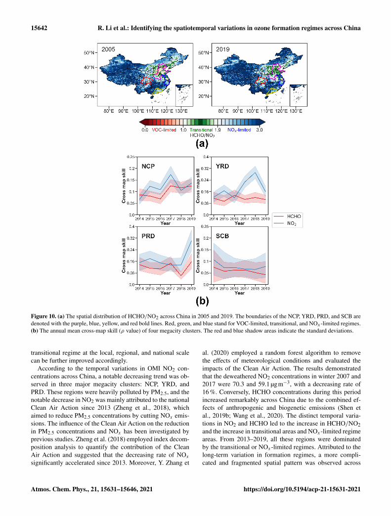
were 26 %, 16 %, and 6 %, respectively. Areas with the tran-sitional regime were mainly distributed in the marginal re-gions of those megacity clusters and scatteredly distributed inthe SCB. Areas with the transitional regime occupied 60 %,50 %, 14 %, and 20 % in the NCP, YRD, PRD, and SCB.The NOx-limited regime dominated other areas (Fig. 10a). In2019, areas with the VOC-limited regime decreased signifi-cantly; this regime was simply found in the fringe areas of theNCP and YRD. The proportion of the VOC-limited regime inthe NCP and YRD was 2 % and 9 %, respectively. The tran-sitional regime was widely distributed throughout the NCP,YRD, and SCB and occupied 71 %, 56 %, and 36 % of thetotal areas. The NOx-limited regime still spread over a ma-jority of China (Fig. 10a). We calculated the annual mean ρof HCHO and NO2 over those megacity clusters from 2014to 2019 (Fig. 10b). For all megacity clusters, the ρ of NO2was higher than HCHO, indicating that NO2 was the dom-inant factor for surface ozone concentrations. Both modelssuggested that NO2 played a more important role in affectingsurface ozone concentrations than HCHO. In the past severalyears, NOx-oriented emission reduction has been conductedacross China, leading to the continuous decrease in NOx con-centrations. Since both VOCs and NOx imposed positive in-fluences on surface ozone concentrations under the transi-tional and NOx-limited ozone formation regime, the upwardtrend of HCHO across China might explain recent soaringozone concentrations across China (Shen et al., 2019a; Luet al., 2020). It is noted that the difference between the ρ ofNO2 and HCHO decreased notably in the NCP and YRD.This may be attributed to the following reason. The NCP andYRD are the regions that received severe PM2.5 pollution,and strict NOx reduction policies have been conducted since2013. With the remarkably reduced NO2 concentrations, thevariations in HCHO concentrations plays an increasingly im-portant role in affecting ozone concentrations in the NCP andYRD. The reduction in VOC emissions is key for an effec-tive management of surface ozone pollution in the NCP andYRD.

3.4 Variations in ozone formation regimes in urbanand rural areas

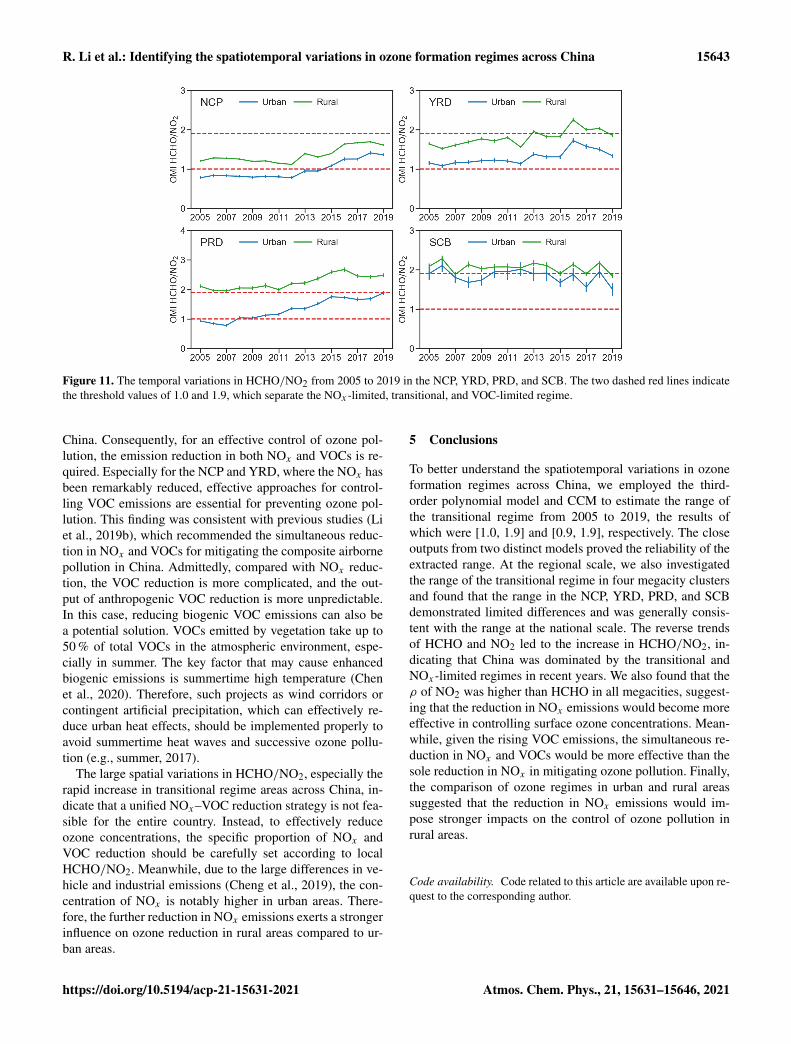
Previous studies suggested that the differences in ozone for-mation regimes existed between urban and rural areas (Tonget al., 2017; Y. Liu et al., 2018; Cheng et al., 2019). We ex-tracted HCHO and NO2 columns in urban and rural pixels inthose megacity clusters and calculated the annually averagedHCHO/NO2 (Fig. 11). For the NCP, HCHO/NO2 in urbanareas was higher than 1.0 since 2015, indicating a transfor-mation from the VOC-limited to the transitional regime. Theincrease in HCHO/NO2 was attributed to the reversed vari-ation trends of HCHO and NO2. The rising HCHO resultedfrom the increase in anthropogenic emissions and biogenicvolatile organic compounds (BVOCs) (Shen et al., 2019b;Wang et al., 2020), while the implementation of the Clean Air

Action imposed notable influences on the decrease in NO2(Chen et al., 2019a). HCHO/NO2 in rural areas was in therange of [1.0, 1.9], indicating that rural areas were occupiedby the transitional regime from 2005 to 2019. For the YRD,which was occupied by the transitional regime, no variationin ozone formation regime was found in urban areas. In ru-ral areas, HCHO/NO2 temporally exceeded the thresholdof 1.9 from 2016 to 2018, indicating that the ozone forma-tion regime changed from transitional to NOx-limited. Thisphenomenon was attributed to the slight decline in HCHO,which might be attributed to the restrictions on crop residueburning in this area (Zhuang et al., 2018; Shen et al., 2019b).Due to the large differences in NO2 concentrations, the urbanand rural areas in the PRD were dominated by the transitionalregime and NOx-limited regime. For the SCB, HCHO/NO2in both urban and rural areas fluctuated around the thresholdvalue of 1.9, and no significant difference between urban andrural areas was found.

4 Discussion

This research employed CCM and a third-order polynomialmodel to estimate the transitional regime of ozone formationacross China, and the calculated range of HCHO/NO2 was[0.9, 1.9] and [1.0, 1.9], respectively. Our findings were gen-erally consistent with previous studies. For the US, Duncanet al. (2010) and Choi et al. (2012) employed the OMI andGOME-2 data, whose 0.25◦ resolution was close to this re-search, and calculated the range of the transitional regimeas [1.0, 2.0]. The similar range of the transitional regime inthe US and China further proved the reliability of the calcu-lated range [1.0, 1.9] at a national scale. On the other hand,the range of the transitional regime can vary significantlyacross regions (Schroeder et al., 2017; Jin et al., 2020). Sunet al. (2018) employed station-based data and calculated therange of the transitional regime in Anhui Province, China,as [1.3, 2.8], which was notably higher than the range acrossChina. Jin et al. (2020) calculated the range of the transi-tional regime in several major regions in the US using theQA4ECV dataset, whose spatial resolution was 0.125◦, andthe output [3.2, 4.1] was much larger than the averaged rangeof the transitional regime across the US. One reason couldbe the severe ozone pollution in megacities, leading to dif-ferent ranges of the transitional regime. Meanwhile, the cal-culated range of the transitional regime is closely related tothe spatial resolution of employed HCHO and NO2 data, andhigh-resolution data are more advantageous in extracting thesensitivity of ozone concentrations to precursors at the localscale (Martin et al., 2004; Jin et al., 2017, 2020). In addi-tion to the generally consistent outputs, some advances ofthis research are listed as follows. First, only a few parame-ters are required for the polynomial model and CCM, whicheffectively reduced the uncertainties in model setting. Sec-ond, considering the differences between model and satellite-

Atmos. Chem. Phys., 21, 15631–15646, 2021 https://doi.org/10.5194/acp-21-15631-2021

R. Li et al.: Identifying the spatiotemporal variations in ozone formation regimes across China 15641

Figure 9. The time series of HCHO/NO2 in the four megacity clusters from 2005 to 2019. Black lines indicate the linear trend ofHCHO/NO2. Red, green, and blue dots stand for VOC-limited, transitional, and NOx -limited regimes, respectively.

retrieved datasets (Jin et al., 2020), only observation datawere employed in this research, which reduced potential datainconsistences and uncertainties. Most importantly, given thelack of actual reference data, this research employed two dif-ferent models to examine ozone formation regimes, and theclose outputs further proved the reliability of this research.

Despite a generally reliable output, some uncertainties ex-ist. First, the accuracy of the estimated range of the transi-tional regime might be influenced by the scaling biases be-tween station-based observations of surface ozone and space-based HCHO and NO2. Since ozone monitoring stationsare mainly distributed in urban areas, and a 0.25◦× 0.25◦

grid might cover both the urban and rural areas, the sur-face ozone concentrations of a grid may be overestimated.Second, the uncertainties in OMI HCHO and NO2 datasetsmight impose negative influences on the estimation of thetransitional regime range (Duncan et al., 2010; Jin et al.,2017, 2020; Schroeder et al., 2017). On one hand, errorsexist in the retrieval of HCHO and NO2 vertical columns.On the other hand, vertical mixing was not homogeneous,weakening the capability of using HCHO and NO2 verticalcolumns to explore the near-surface ozone–precursor sensi-tivity. Therefore, future improvement of earth observationtechniques and the spatiotemporal resolution of HCHO andNO2 products can further enhance the accuracy of the esti-mated range of the transitional regime. In general, accordingto the cross-verification and comparison with previous stud-

ies, [1.0, 1.9] from this research is a reliable range for thetransitional ozone formation regime across China and can beused as an approximate criterion to follow when implement-ing national emission reduction policies. On the other hand,given the potential variations in transitional regimes in differ-ent regions, when conducting small-scale research, the rangeof [1.0, 1.9] may be adapted accordingly based on local data.

Previous studies on the range of ozone formation regimeswere mainly conducted using statistical models or chemicaltransport models. For this research, we employed both a sta-tistical and a causality model to cross-verify the range of thetransitional regimes. Despite a relatively high fitting accu-racy in terms of uncertainties, the findings from these studiescould not be effectively compared or interpreted due to thelack of reliable reference data. To this end, as well as numer-ical models, lab experiments should also be considered to ex-tract a more precise description of the ozone–precursor rela-tionship. With the rapid development of atmospheric science,smog chambers have been increasingly employed to investi-gate complicated interactions between multiple precursors.By setting specific meteorological conditions (e.g., tempera-ture and humidity) and gradually adjusting the proportion ofdifferent precursors, how the proportion of NO2 and HCHOaffects the ozone formation regime can be better explained ina theoretical environment. With more reliable experimentalreference data, the model-based analysis on the range of the

https://doi.org/10.5194/acp-21-15631-2021 Atmos. Chem. Phys., 21, 15631–15646, 2021

15642 R. Li et al.: Identifying the spatiotemporal variations in ozone formation regimes across China

Figure 10. (a) The spatial distribution of HCHO/NO2 across China in 2005 and 2019. The boundaries of the NCP, YRD, PRD, and SCB aredenoted with the purple, blue, yellow, and red bold lines. Red, green, and blue stand for VOC-limited, transitional, and NOx -limited regimes.(b) The annual mean cross-map skill (ρ value) of four megacity clusters. The red and blue shadow areas indicate the standard deviations.

transitional regime at the local, regional, and national scalecan be further improved accordingly.

According to the temporal variations in OMI NO2 con-centrations across China, a notable decreasing trend was ob-served in three major megacity clusters: NCP, YRD, andPRD. These regions were heavily polluted by PM2.5, and thenotable decrease in NO2 was mainly attributed to the nationalClean Air Action since 2013 (Zheng et al., 2018), whichaimed to reduce PM2.5 concentrations by cutting NOx emis-sions. The influence of the Clean Air Action on the reductionin PM2.5 concentrations and NOx has been investigated byprevious studies. Zheng et al. (2018) employed index decom-position analysis to quantify the contribution of the CleanAir Action and suggested that the decreasing rate of NOxsignificantly accelerated since 2013. Moreover, Y. Zhang et

al. (2020) employed a random forest algorithm to removethe effects of meteorological conditions and evaluated theimpacts of the Clean Air Action. The results demonstratedthat the deweathered NO2 concentrations in winter 2007 and2017 were 70.3 and 59.1 µgm−3, with a decreasing rate of16 %. Conversely, HCHO concentrations during this periodincreased remarkably across China due to the combined ef-fects of anthropogenic and biogenetic emissions (Shen etal., 2019b; Wang et al., 2020). The distinct temporal varia-tions in NO2 and HCHO led to the increase in HCHO/NO2and the increase in transitional areas and NOx-limited regimeareas. From 2013–2019, all these regions were dominatedby the transitional or NOx-limited regimes. Attributed to thelong-term variation in formation regimes, a more compli-cated and fragmented spatial pattern was observed across

Atmos. Chem. Phys., 21, 15631–15646, 2021 https://doi.org/10.5194/acp-21-15631-2021

R. Li et al.: Identifying the spatiotemporal variations in ozone formation regimes across China 15643

Figure 11. The temporal variations in HCHO/NO2 from 2005 to 2019 in the NCP, YRD, PRD, and SCB. The two dashed red lines indicatethe threshold values of 1.0 and 1.9, which separate the NOx -limited, transitional, and VOC-limited regime.

China. Consequently, for an effective control of ozone pol-lution, the emission reduction in both NOx and VOCs is re-quired. Especially for the NCP and YRD, where the NOx hasbeen remarkably reduced, effective approaches for control-ling VOC emissions are essential for preventing ozone pol-lution. This finding was consistent with previous studies (Liet al., 2019b), which recommended the simultaneous reduc-tion in NOx and VOCs for mitigating the composite airbornepollution in China. Admittedly, compared with NOx reduc-tion, the VOC reduction is more complicated, and the out-put of anthropogenic VOC reduction is more unpredictable.In this case, reducing biogenic VOC emissions can also bea potential solution. VOCs emitted by vegetation take up to50 % of total VOCs in the atmospheric environment, espe-cially in summer. The key factor that may cause enhancedbiogenic emissions is summertime high temperature (Chenet al., 2020). Therefore, such projects as wind corridors orcontingent artificial precipitation, which can effectively re-duce urban heat effects, should be implemented properly toavoid summertime heat waves and successive ozone pollu-tion (e.g., summer, 2017).

The large spatial variations in HCHO/NO2, especially therapid increase in transitional regime areas across China, in-dicate that a unified NOx–VOC reduction strategy is not fea-sible for the entire country. Instead, to effectively reduceozone concentrations, the specific proportion of NOx andVOC reduction should be carefully set according to localHCHO/NO2. Meanwhile, due to the large differences in ve-hicle and industrial emissions (Cheng et al., 2019), the con-centration of NOx is notably higher in urban areas. There-fore, the further reduction in NOx emissions exerts a strongerinfluence on ozone reduction in rural areas compared to ur-ban areas.

5 Conclusions

To better understand the spatiotemporal variations in ozoneformation regimes across China, we employed the third-order polynomial model and CCM to estimate the range ofthe transitional regime from 2005 to 2019, the results ofwhich were [1.0, 1.9] and [0.9, 1.9], respectively. The closeoutputs from two distinct models proved the reliability of theextracted range. At the regional scale, we also investigatedthe range of the transitional regime in four megacity clustersand found that the range in the NCP, YRD, PRD, and SCBdemonstrated limited differences and was generally consis-tent with the range at the national scale. The reverse trendsof HCHO and NO2 led to the increase in HCHO/NO2, in-dicating that China was dominated by the transitional andNOx-limited regimes in recent years. We also found that theρ of NO2 was higher than HCHO in all megacities, suggest-ing that the reduction in NOx emissions would become moreeffective in controlling surface ozone concentrations. Mean-while, given the rising VOC emissions, the simultaneous re-duction in NOx and VOCs would be more effective than thesole reduction in NOx in mitigating ozone pollution. Finally,the comparison of ozone regimes in urban and rural areassuggested that the reduction in NOx emissions would im-pose stronger impacts on the control of ozone pollution inrural areas.

Code availability. Code related to this article are available upon re-quest to the corresponding author.

https://doi.org/10.5194/acp-21-15631-2021 Atmos. Chem. Phys., 21, 15631–15646, 2021

15644 R. Li et al.: Identifying the spatiotemporal variations in ozone formation regimes across China

Data availability. The OMI HCHO and NO2 can be obtained fromhttps://disc.gsfc.nasa.gov/ (GES DISC, 2021). The surface ozonenetwork data are available at https://quotsoft.net/air (Wang, 2021).The MODIS land cover product can be accessed from https://earthdata.nasa.gov/ (NASA, 2021).

Author contributions. RL performed the analysis and wrote the ini-tial draft of the manuscript. ZC and ML designed the study and re-viewed the paper. MX provided satellite data, tools. QY providedsurface ozone network data. NZ and BG contributed to the interpre-tation of the results. All authors made substantial contributions tothis work.

Competing interests. The authors declare that they have no conflictof interest.

Disclaimer. Publisher’s note: Copernicus Publications remainsneutral with regard to jurisdictional claims in published maps andinstitutional affiliations.

Acknowledgements. This research is supported by the Beijing Nat-ural Science Foundation (grant no. 8202031), the Open Fund of theState Key Laboratory of Remote Sensing Science (grant no. OF-SLRSS201926), the Open Fund of the State Key Laboratory of Re-sources and Environmental Information System, and the Fundamen-tal Research Funds for the Central Universities.

Financial support. This research has been supported by the Bei-jing Municipal Natural Science Foundation (grant no. 8202031), theOpen Fund of the State Key Laboratory of Remote Sensing Science(grant no. OFSLRSS201926), the Open Fund of the State Key Lab-oratory of Resources and Environmental Information System, andthe the Fundamental Research Funds for the Central Universities.

Review statement. This paper was edited by Xavier Querol and re-viewed by two anonymous referees.

References

Bajocco, S., Smiraglia, D., Scaglione, M., Raparelli, E., and Sal-vati, L.: Exploring the role of land degradation on agriculturalland use change dynamics, Sci. Total Environ., 636, 1373–1381,https://doi.org/10.1016/j.scitotenv.2018.04.412, 2018.

Bucsela, E. J., Krotkov, N. A., Celarier, E. A., Lamsal, L. N.,Swartz, W. H., Bhartia, P. K., Boersma, K. F., Veefkind, J. P.,Gleason, J. F., and Pickering, K. E.: A new stratospheric andtropospheric NO2 retrieval algorithm for nadir-viewing satelliteinstruments: applications to OMI, Atmos. Meas. Tech., 6, 2607–2626, https://doi.org/10.5194/amt-6-2607-2013, 2013.

Chang, C.-Y., Faust, E., Hou, X., Lee, P., Kim, H. C.,Hedquist, B. C., and Liao, K.-J.: Investigating ambient ozone

formation regimes in neighboring cities of shale plays inthe Northeast United States using photochemical model-ing and satellite retrievals, Atmos. Environ., 142, 152–170,https://doi.org/10.1016/j.atmosenv.2016.06.058, 2016.

Chen, Z., Xie, X., Cai, J., Chen, D., Gao, B., He, B., Cheng, N., andXu, B.: Understanding meteorological influences on PM2.5 con-centrations across China: a temporal and spatial perspective, At-mos. Chem. Phys., 18, 5343–5358, https://doi.org/10.5194/acp-18-5343-2018, 2018.

Chen, Z., Chen, D., Kwan, M.-P., Chen, B., Gao, B., Zhuang, Y.,Li, R., and Xu, B.: The control of anthropogenic emissions con-tributed to 80 % of the decrease in PM2.5 concentrations in Bei-jing from 2013 to 2017, Atmos. Chem. Phys., 19, 13519–13533,https://doi.org/10.5194/acp-19-13519-2019, 2019a.

Chen, Z., Chen, D., Wen, W., Zhuang, Y., Kwan, M.-P., Chen, B.,Zhao, B., Yang, L., Gao, B., Li, R., and Xu, B.: Evaluating the“2+26” regional strategy for air quality improvement during twoair pollution alerts in Beijing: variations in PM2.5 concentrations,source apportionment, and the relative contribution of local emis-sion and regional transport, Atmos. Chem. Phys., 19, 6879–6891,https://doi.org/10.5194/acp-19-6879-2019, 2019b.

Chen, Z., Zhuang, Y., Xie, X., Chen, D., Cheng, N., Yang,L., and Li, R.: Understanding long-term variations of me-teorological influences on ground ozone concentrations inBeijing during 2006-2016, Environ. Pollut., 245, 29–37,https://doi.org/10.1016/j.envpol.2018.10.117, 2019c.

Chen, Z., Li, R., Chen, D., Zhuang, Y., Gao, B., Yang,L., and Li, M.: Understanding the causal influence ofmajor meteorological factors on ground ozone con-centrations across China, J. Clean. Prod., 242, 118498,https://doi.org/10.1016/j.jclepro.2019.118498, 2020.

Cheng, N., Chen, Z., Sun, F., Sun, R., Dong, X., Xie, X.,and Xu, C.: Ground ozone concentrations over Beijing from2004 to 2015: Variation patterns, indicative precursors and ef-fects of emission-reduction, Environ. Pollut., 237, 262–274,https://doi.org/10.1016/j.envpol.2018.02.051, 2018.

Cheng, N., Li, R., Xu, C., Chen, Z., Chen, D., Meng, F.,Cheng, B., Ma, Z., Zhuang, Y., He, B., and Gao, B.:Ground ozone variations at an urban and a rural stationin Beijing from 2006 to 2017: Trend, meteorological influ-ences and formation regimes, J. Clean. Prod., 235, 11–20,https://doi.org/10.1016/j.jclepro.2019.06.204, 2019.

Choi, Y., Kim, H., Tong, D., and Lee, P.: Summertime weeklycycles of observed and modeled NOx and O3 concentrationsas a function of satellite-derived ozone production sensitivityand land use types over the Continental United States, At-mos. Chem. Phys., 12, 6291–6307, https://doi.org/10.5194/acp-12-6291-2012, 2012.

Duncan, B. N., Yoshida, Y., Olson, J. R., Sillman, S., Martin,R. V., Lamsal, L., Hu, Y., Pickering, K. E., Retscher, C.,Allen, D. J., and Crawford, J. H.: Application of OMI obser-vations to a space-based indicator of NOx and VOC controlson surface ozone formation, Atmos. Environ., 44, 2213–2223,https://doi.org/10.1016/j.atmosenv.2010.03.010, 2010.

Gehan, E. A.: A generalized Wilcoxon test for comparing ar-bitrarily singly-censored samples, Biometrika, 52, 203–224,https://doi.org/10.1093/biomet/52.1-2.203, 1965.

Atmos. Chem. Phys., 21, 15631–15646, 2021 https://doi.org/10.5194/acp-21-15631-2021

R. Li et al.: Identifying the spatiotemporal variations in ozone formation regimes across China 15645

GES DISC: The OMI satellite data for NO2 and HCHO, NASA[data set], available at: https://disc.gsfc.nasa.gov/, last access: 1September 2021.

González Abad, G., Liu, X., Chance, K., Wang, H., Kurosu,T. P., and Suleiman, R.: Updated Smithsonian Astrophysi-cal Observatory Ozone Monitoring Instrument (SAO OMI)formaldehyde retrieval, Atmos. Meas. Tech., 8, 19–32,https://doi.org/10.5194/amt-8-19-2015, 2015.

Imhoff, M. L., Zhang, P., Wolfe, R. E., and Bounoua, L.: Re-mote sensing of the urban heat island effect across biomes inthe continental USA, Remote Sens. Environ., 114, 504–513,https://doi.org/10.1016/j.rse.2009.10.008, 2010.

Jin, X. and Holloway, T.: Spatial and temporal variability ofozone sensitivity over China observed from the Ozone Mon-itoring Instrument, J. Geophys. Res.-Atmos., 120, 7229–7246,https://doi.org/10.1002/2015JD023250, 2015.

Jin, X., Fiore, A. M., Murray, L. T., Valin, L. C., Lamsal, L. N.,Duncan, B., Boersma, K. F., De Smedt, I., Abad, G. G., Chance,K., and Tonnesen, G. S.: Evaluating a Space-Based Indicator ofSurface Ozone-NOx -VOC Sensitivity Over Midlatitude SourceRegions and Application to Decadal Trends, J. Geophys. Res.-Atmos., 122, 10–461, https://doi.org/10.1002/2017JD026720,2017.

Jin, X., Fiore, A., Boersma, K. F., De Smedt, I., and Valin, L.: Infer-ring changes in summertime surface ozone-NOx -VOC chemistryover U.S. urban areas from two decades of satellite and ground-based observations, Environ. Sci. Technol., 54, 11, 6518–6529,https://doi.org/10.1021/acs.est.9b07785, 2020.

Kendall, M.: Rank Correlation Methods, Theory and applicationsof rank order-statistics, Griffin, London, 202 pp., 1970.

Kleinman, L. I.: Low and high NOx tropospheric pho-tochemistry, J. Geophys. Res.-Atmos., 99, 16831–16838,https://doi.org/10.1029/94JD01028, 1994.

Kroon, M., De Haan, J., Veefkind, J., Froidevaux, L., Wang, R.,Kivi, R., and Hakkarainen, J.: Validation of operational ozoneprofiles from the Ozone Monitoring Instrument, J. Geophys.Res.-Atmos., 116, https://doi.org/10.1029/2010JD015100, 2011.

Krotkov, N. A., Lamsal, L. N., Celarier, E. A., Swartz, W. H.,Marchenko, S. V., Bucsela, E. J., Chan, K. L., Wenig, M.,and Zara, M.: The version 3 OMI NO2 standard product, At-mos. Meas. Tech., 10, 3133–3149, https://doi.org/10.5194/amt-10-3133-2017, 2017.

Lamsal, L. N., Krotkov, N. A., Celarier, E. A., Swartz, W. H.,Pickering, K. E., Bucsela, E. J., Gleason, J. F., Martin, R. V.,Philip, S., Irie, H., Cede, A., Herman, J., Weinheimer, A., Szyk-man, J. J., and Knepp, T. N.: Evaluation of OMI operationalstandard NO2 column retrievals using in situ and surface-basedNO2 observations, Atmos. Chem. Phys., 14, 11587–11609,https://doi.org/10.5194/acp-14-11587-2014, 2014.

Levelt, P. F., van den Oord, G. H., Dobber, M. R., Malkki, A.,Visser, H., de Vries, J., Stammes, P., Lundell, J. O., and Saari, H.:The ozone monitoring instrument, IEEE T. Geosci. Remote, 44,1093–1101, https://doi.org/10.1109/TGRS.2006.872333, 2006.

Li, K., Jacob, D. J., Liao, H., Shen, L., Zhang, Q., and Bates, K.H.: Anthropogenic drivers of 2013-2017 trends in summer sur-face ozone in China, P. Natl. Acad. Sci. USA, 116, 422–427,https://doi.org/10.1073/pnas.1812168116, 2019a.

Li, K., Jacob, D. J., Liao, H., Zhu, J., Shah, V., Shen, L., Bates, K.H., Zhang, Q., and Zhai, S.: A two-pollutant strategy for improv-

ing ozone and particulate air quality in China, Nat. Geosci., 12,906–910, https://doi.org/10.1038/s41561-019-0464-x, 2019b.

Li, K., Jacob, D. J., Shen, L., Lu, X., De Smedt, I., and Liao,H.: Increases in surface ozone pollution in China from 2013to 2019: anthropogenic and meteorological influences, Atmos.Chem. Phys., 20, 11423–11433, https://doi.org/10.5194/acp-20-11423-2020, 2020.

Liu, H., Liu, S., Xue, B., Lv, Z., Meng, Z., Yang, X., Xue,T., Yu, Q., and He, K.: Ground-level ozone pollution andits health impacts in China, Atmos. Environ., 173, 223–230,https://doi.org/10.1016/j.atmosenv.2017.11.014, 2018.

Liu, Y., Li, L., An, J., Huang, L., Yan, R., Huang, C., Wang, H.,Wang, Q., Wang, M., and Zhang, W.: Estimation of biogenicVOC emissions and its impact on ozone formation over theYangtze River Delta region, China, Atmos. Environ. 186, 113–128, https://doi.org/10.1016/j.atmosenv.2018.05.027, 2018.

Lu, X., Zhang, L., Wang, X., Gao, M., Li, K., Zhang,Y., Yue, X., and Zhang, Y.: Rapid Increases in warm-season surface ozone and resulting health impact inChina Since 2013, Environ. Sci. Tech. Let., 7, 240–247,https://doi.org/10.1021/acs.estlett.0c00171, 2020.

Martin, R. V., Fiore, A. M., and Van Donkelaar, A.: Space-based diagnosis of surface ozone sensitivity to anthro-pogenic emissions, Geophys. Res. Lett., 31, L06120,https://doi.org/10.1029/2004GL019416, 2004.

Milford, J. B., Russell, A. G., and McRae, G. J.: A new approachto photochemical pollution control: Implications of spatial pat-terns in pollutant responses to reductions in nitrogen oxides andreactive organic gas emissions, Environ. Sci. Technol., 23, 1290–1301, https://doi.org/10.1021/es00068a017, 1989.

NASA: Earthdata, NASA [data set], available at: https://earthdata.nasa.gov/, last access: 1 September 2021.

Palmer, S. C., Odermatt, D., Hunter, P., Brockmann, C., Presing,M., Balzter, H., and Tóth, V.: Satellite remote sensing ofphytoplankton phenology in Lake Balaton using 10 years ofMERIS observations, Remote Sens. Environ., 158, 441–452,https://doi.org/10.1016/j.rse.2014.11.021, 2015.

Peng, J., Ma, J., Liu, Q., Liu, Y., Hu, Y., Li, Y., and Yue, Y.: Spatial-temporal change of land surface temperature across 285 cities inChina: An urban-rural contrast perspective, Sci. Total Environ.,635, 487–497, https://doi.org/10.1016/j.scitotenv.2018.04.105,2018.

Pusede, S. E. and Cohen, R. C.: On the observed response of ozoneto NOx and VOC reactivity reductions in San Joaquin ValleyCalifornia 1995–present, Atmos. Chem. Phys., 12, 8323–8339,https://doi.org/10.5194/acp-12-8323-2012, 2012.

Schroeder, J. R., Crawford, J. H., Fried, A., Walega, J., Wein-heimer, A., Wisthaler, A., Müller, M., Mikoviny, T., Chen, G.,Shook, M., Blake, D. R., and Tonnesen, G. S.: New insightsinto the column CH2O/NO2 ratio as an indicator of near-surfaceozone sensitivity, J. Geophys. Res.-Atmos., 122, 8885–8907,https://doi.org/10.1002/2017JD026781, 2017.

Shen, L., Jacob, D. J., Liu, X., Huang, G., Li, K., Liao, H., andWang, T.: An evaluation of the ability of the Ozone Monitor-ing Instrument (OMI) to observe boundary layer ozone pollu-tion across China: application to 2005–2017 ozone trends, At-mos. Chem. Phys., 19, 6551–6560, https://doi.org/10.5194/acp-19-6551-2019, 2019a.

https://doi.org/10.5194/acp-21-15631-2021 Atmos. Chem. Phys., 21, 15631–15646, 2021

15646 R. Li et al.: Identifying the spatiotemporal variations in ozone formation regimes across China

Shen, L., Jacob, D. J., Zhu, L., Zhang, Q., Zheng, B., Sulprizio,M. P., Li, K., De Smedt, I., González Abad, G., Cao, H., Fu,T. M., and Liao, H.: The 2005–2016 Trends of formaldehydecolumns over China observed by satellites: Increasing anthro-pogenic emissions of volatile organic compounds and decreasingagricultural fire emissions, Geophys. Res. Lett., 46, 4468–4475,https://doi.org/10.1029/2019GL082172, 2019b.

Sillman, S., Logan, J. A., and Wofsy, S. C.: The sensitivityof ozone to nitrogen oxides and hydrocarbons in regionalozone episodes, J. Geophys. Res.-Atmos., 95, 1837–1851,https://doi.org/10.1029/JD095iD02p01837, 1990.

Sugihara, G., May, R., Ye, H., Hsieh, C.-H., Deyle, E., Fogarty, M.,and Munch, S.: Detecting causality in complex ecosystems, Sci-ence, 338, 496–500, https://doi.org/10.1126/science.1227079,2012.

Sun, Y., Liu, C., Palm, M., Vigouroux, C., Notholt, J., Hu, Q., Jones,N., Wang, W., Su, W., Zhang, W., Shan, C., Tian, Y., Xu, X., DeMazière, M., Zhou, M., and Liu, J.: Ozone seasonal evolutionand photochemical production regime in the polluted tropospherein eastern China derived from high-resolution Fourier trans-form spectrometry (FTS) observations, Atmos. Chem. Phys.,18, 14569–14583, https://doi.org/10.5194/acp-18-14569-2018,2018.

Tong, L., Zhang, H., Yu, J., He, M., Xu, N., Zhang, J.,Qian, F., Feng, J., and Xiao, H.: Characteristics of sur-face ozone and nitrogen oxides at urban, suburban andrural sites in Ningbo, China, Atmos. Res., 187, 57–68,https://doi.org/10.1016/j.atmosres.2016.12.006, 2017.

Wang, H., Wu, Q., Guenther, A. B., Yang, X., Wang, L., Xiao,T., Li, J., Feng, J., Xu, Q., and Cheng, H.: A long-term esti-mation of biogenic volatile organic compound (BVOC) emis-sion in China from 2001–2016: the roles of land cover changeand climate variability, Atmos. Chem. Phys., 21, 4825–4848,https://doi.org/10.5194/acp-21-4825-2021, 2021.

Wang, J., Li, X., Christakos, G., Liao, Y., Zhang, T., Gu, X.,and Zheng, X.: Geographical detectors-based health risk assess-ment and its application in the neural tube defects study of theHeshun region, China, Int. J. Geogr. Inf. Sci., 24, 107–127,https://doi.org/10.1080/13658810802443457, 2010.

Wang, J., Zhang, T., and Fu, B.: A measure of spa-tial stratified heterogeneity, Ecol. Indic., 67, 250–256,https://doi.org/10.1016/j.ecolind.2016.02.052, 2016.

Wang, T., Xue, L., Brimblecombe, P., Lam, Y. F., Li, L.,and Zhang, L.: Ozone pollution in China: A review ofconcentrations, meteorological influences, chemical precur-sors, and effects, Sci. Total Environ., 575, 1582–1596,https://doi.org/10.1016/j.scitotenv.2016.10.081, 2017.

Wang, T., Dai, J., Lam, K. S., Nan Poon, C., and Brasseur,G. P.: Twenty-five years of lower tropospheric ozone ob-servations in tropical East Asia: The influence of emissionsand weather patterns, Geophys. Res. Lett., 46, 11463–11470,https://doi.org/10.1029/2019GL084459, 2019.

Wang, X. L.: Historical air quality data in China, Quotsoft [dataset], available at: https://quotsoft.net/air, last access: 1 September2021.

Wu, R. and Xie, S.: Spatial distribution of ozone formationin China derived from emissions of speciated volatile or-ganic compounds, Environ. Sci. Technol., 51, 2574–2583,https://doi.org/10.1021/acs.est.6b03634, 2017.

Xie, Y., Dai, H., Zhang, Y., Wu, Y., Hanaoka, T., and Masui,T.: Comparison of health and economic impacts of PM2.5and ozone pollution in China, Environ. Int., 130, 104881,https://doi.org/10.1016/j.envint.2019.05.075, 2019.

Yao, R., Wang, L., Huang, X., Gong, W., and Xia, X.:Greening in rural areas increases the surface urban heatisland intensity, Geophys. Res. Lett., 46, 2204–2212,https://doi.org/10.1029/2018GL081816, 2019.

Zeb, N., Khokhar, M. F., Pozzer, A., and Khan, S. A.: Ex-ploring the temporal trends and seasonal behaviour oftropospheric trace gases over Pakistan by exploitingsatellite observations, Atmos. Environ., 198, 279–290,https://doi.org/10.1016/j.atmosenv.2018.10.053, 2019.

Zhang, X., Zhao, L., Cheng, M., and Chen, D.: Estimating ground-level ozone concentrations in eastern China using satellite-basedprecursors, IEEE Trans. Geosci. Remote Sens., 58, 4754–4763,https://doi.org/10.1109/TGRS.2020.2966780, 2020.

Zhang, Y., Vu, T. V., Sun, J., He, J., Shen, X., Lin, W., Zhang,X., Zhong, J., Gao, W., Wang, Y., Fu, T. M., Ma, Y., Li,W., and Shi, Z.: Significant changes in chemistry of fineparticles in wintertime Beijing from 2007 to 2017: Impactof clean air actions, Environ. Sci. Technol., 54, 1344–1352,https://doi.org/10.1021/acs.est.9b04678, 2020.

Zheng, B., Tong, D., Li, M., Liu, F., Hong, C., Geng, G., Li, H., Li,X., Peng, L., Qi, J., Yan, L., Zhang, Y., Zhao, H., Zheng, Y., He,K., and Zhang, Q.: Trends in China’s anthropogenic emissionssince 2010 as the consequence of clean air actions, Atmos. Chem.Phys., 18, 14095–14111, https://doi.org/10.5194/acp-18-14095-2018, 2018.

Zhu, L., Jacob, D. J., Mickley, L. J., Marais, E. A., Cohan, D. S.,Yoshida, Y., Duncan, B. N., Abad, G. G., and Chance, K. V.: An-thropogenic emissions of highly reactive volatile organic com-pounds in eastern Texas inferred from oversampling of satellite(OMI) measurements of HCHO columns, Environ. Sci. Tech.Let., 9, 114004, https://doi.org/10.1088/1748-9326/9/11/114004,2014.

Zhu, L., Mickley, L. J., Jacob, D. J., Marais, E. A., Sheng, J., Hu,L., Abad, G. G., and Chance, K.: Long-term (2005–2014) trendsin formaldehyde (HCHO) columns across North America as seenby the OMI satellite instrument: Evidence of changing emissionsof volatile organic compounds, Geophys. Res. Lett., 44, 7079–7086, https://doi.org/10.1002/2017GL073859, 2017.

Zhuang, Y., Li, R., Yang, H., Chen, D., Chen, Z., Gao, B., andHe, B.: Understanding temporal and spatial distribution of cropresidue burning in China from 2003 to 2017 using MODIS data,Remote Sens., 10, 390, https://doi.org/10.3390/rs10030390,2018.

Atmos. Chem. Phys., 21, 15631–15646, 2021 https://doi.org/10.5194/acp-21-15631-2021