idsl: automated performance prediction and analysis of ... · viz., image processing of ixr...

iDSL: Automated Performance Predictionand Analysis of Medical Imaging Systems

Freek van den Berg(B), Anne Remke, and Boudewijn R. Haverkort

University of Twente, PO Box 217, 7500 AE Enschede, The Netherlands{f.g.b.vandenberg,a.k.i.remke,b.r.h.m.haverkort}@utwente.nl

Abstract. iDSL is a language and toolbox for performance prediction ofMedical Imaging Systems; It enables system designers to automaticallyevaluate the performance of their designs, using advanced means of modelchecking and simulation techniques under the hood, and presents resultsgraphically. In this paper, we present a performance evaluation approachbased on iDSL that (i) relies on few measurements; (ii) evaluates manydifferent design alternatives (so-called “designs”); (iii) provides under-standable metrics; and (iv) is applicable to real complex systems. Nextto that, iDSL supports advanced methods for model calibration as wellas ways to aggregate performance results. An extensive case study oninterventional X-ray systems shows that iDSL can be used to study theimpact of different hardware platforms and concurrency choices on theoverall system performance. Model validation conveys that the predictedresults closely reflect reality.

1 Introduction

Embedded systems have faced a significant increase in complexity over timeand are confronted with stringent costs constraints. They are frequently usedto perform safety critical tasks, as with Medical Imaging Systems (MIS). Theirsafety is significantly determined by their performance. As an example of animportant class of MIS, we consider interventional X-ray (iXR) systems, as builtand designed by Philips Healthcare.

These systems create images continuously based on X-ray beams, which areobserved by a surgeon operating a patient. Images need to be shown quickly forhand-eye coordination [14], viz., the surgeon perceives images to be real-time.

In earlier work, when the ASD method [10] was considered to be used for thedesign of iXR machines, we have evaluated their performance using simulationmodels, derived from the design specification by hand.

This paper presents a fully formalised performance evaluation trajectory inwhich we go from real measurements, via a formal model, to performance pre-dictions, for many different designs, in a fully automated way. Starting point

This research was supported as part of the Dutch national program COMMIT, andcarried out as part of the Allegio project under the responsibility of the ESI groupof TNO, with Philips Medical Systems B.V. as the carrying industrial partner.

c© Springer International Publishing Switzerland 2015M. Beltran et al. (Eds.): EPEW 2015, LNCS 9272, pp. 227–242, 2015.DOI: 10.1007/978-3-319-23267-6 15

228 F. van den Berg et al.

for this evaluation are models expressed in the IDSL formalism, which has beenintroduced in [4] and is extended here to fit our new approach. From such mod-els input for the Modest toolset [11] is automatically generated and results arevisualized using Graphviz and Gnuplot. This is not only very efficient, it alsobrings advanced formal performance evaluation techniques, e.g., based on modelchecking of timed automata and Markov chains, and discrete-event simulation,at the fingertips of system designers, without bothering them with the technicaldetails of these. Furthermore, the approach allows to efficiently predict the per-formance of a large number of design variants, to compare them, and select thebest design given a set of constraints and measures of interest. However, notethat in contrast to Design Space Exploration (DSE) [2], in which a few optimaldesigns are being searched for, we evaluated a large and fixed amount of designs.

Even though the presented approach is fairly general, we illustrate its fea-sibility on so-called biplane iXR systems, which comprise two imaging chains,positioned in perpendicular planes to enable 3D-imaging. They are currentlyimplemented using two separate hardware platforms. However, for various rea-sons, e.g., costs, physical space, energy consumption and failure rate, it is worthinvestigating running the software for both image chains on shared (but morepowerful) hardware. Hence, we use the above mentioned approach to predict theperformance for shared hardware as a case study. Sharing hardware gives poten-tial to concurrency, which may result in increased latency and jitter of images,which, in their turn, affect (perceived) system safety.

We have identified four key objectives that such an integral and fully auto-mated performance evaluation approach should meet, i.e., it should

O1: use as few costly measurements as possible;O2: be able to evaluate a large number of complex designs;O3: present its predictions intuitively via understandable (aggregated) metrics;O4: be applicable to real complex systems.

These objectives are realized through the following four contributions made inthis paper. First, the model is calibrated using measurements and measurementpredictions to rely on few costly measurements. In contrast, current Design SpaceExploration approaches typically require many measurements to be readily avail-able [2,13]. Second, we use iDSL [4], a language and toolbox for automated per-formance evaluation of service systems, and extend it to support the predictionof unseen empirical cumulative distribution functions (eCDFs). The automationallows us to evaluate many designs, using Modest [11] for simulations, in line withprevious work [5,12]. Third, we use a variety of aggregation functions to evaluatedesigns on different aspects. Fourth, we conduct a case study on a real-life MIS,viz., Image Processing of iXR systems. We validate our model by comparing itspredictions with corresponding measurements. Also, the predictions are used togain insight in the performance of biplane iXR systems with shared hardware.

iDSL: Automated Performance Prediction and Analysis 229

Paper Outline: This paper is organised as follows: Section 2 provides themethodology of our approach. Section 3 describes how measurements are taken,predicted and applied. Section 4 sketches the iDSL tool chain and model. Section5 presents the results of the case study. Section 6 concludes the paper.

2 Methodology

Fig. 1. The solution chain of the approachcomprising pre-processing (performing mea-surements and deriving execution times), pro-cessing (predicting eCDFs and simulating)and post-processing (aggregate functions).

We specify our approach as a solu-tion chain as depicted in Figure 1,consisting of three consecutivestages, viz., pre-processing, pro-cessing and post-processing. TheiDSL toolbox automates these stepsand connects them seamlessly.

During pre-processing, mea-surements are performed and exe-cution times derived from them.They are performed for differ-ent iXR system configurations andyield large sets of so-called activ-ities for every single design. Anactivity specifies, for a particularresource and a performed func-tion, the time interval of execution.Activities are visualized automat-ically in Gantt charts [15]. Theyare grouped to obtain total execu-tion times per function and in turnaggregated into so-called empiricalcumulative distribution functions.

During processing, we startwith many inverse eCDFs, all basedon measurements, that cover allpossible designs of interest. Many are used for model validation (explained below)and a fraction of them is used to predict new, inverse eCDFs. Hence, one mayreason about the performance of many designs, while relying on only few mea-surements, in line with Objective O1.

Next, the iDSL model is executed to obtain performance results, in two steps:(i) iDSL predicts eCDFs for all designs and calibrates the model based on theseeCDFs; and (ii) iDSL performs many simulations via the Modest toolset (seeSection 4), yielding results for all designs, meeting Objective O2.

During post-processing, results are processed into aggregated, understand-able metrics, facilitating the interpretation of the results (Objective O3).


3 Measurements and Emperical CDFs

In this section, measurements performed on design instances are used to predictthe performance of other design instances, in four steps: (i) we perform measure-ments that yield activities; (ii) these activities are grouped into execution times;(iii) these execution times are used to estimate emperical CDFs (eCDFs); and(iv) we predict eCDFs for the complete design space, relying on few estimatedeCDFs. We discuss these 4 steps below in more detail.

3.1 Measuring Activities on a Real System

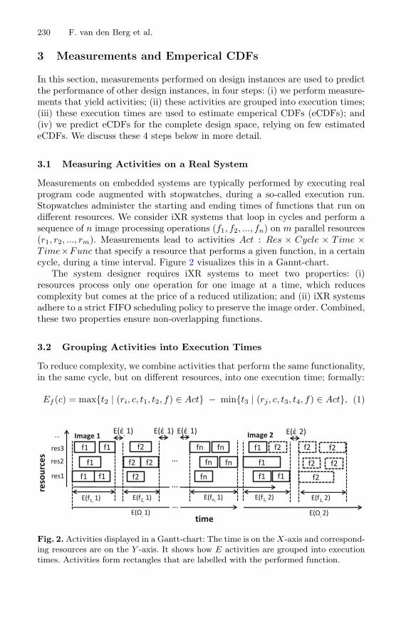
Measurements on embedded systems are typically performed by executing realprogram code augmented with stopwatches, during a so-called execution run.Stopwatches administer the starting and ending times of functions that run ondifferent resources. We consider iXR systems that loop in cycles and perform asequence of n image processing operations (f1, f2, ..., fn) on m parallel resources(r1, r2, ..., rm). Measurements lead to activities Act : Res × Cycle × Time ×Time×Func that specify a resource that performs a given function, in a certaincycle, during a time interval. Figure 2 visualizes this in a Gannt-chart.

The system designer requires iXR systems to meet two properties: (i)resources process only one operation for one image at a time, which reducescomplexity but comes at the price of a reduced utilization; and (ii) iXR systemsadhere to a strict FIFO scheduling policy to preserve the image order. Combined,these two properties ensure non-overlapping functions.

3.2 Grouping Activities into Execution Times

To reduce complexity, we combine activities that perform the same functionality,in the same cycle, but on different resources, into one execution time; formally:

Ef (c) = max{t2 | (ri, c, t1, t2, f) ∈ Act} − min{t3 | (rj , c, t3, t4, f) ∈ Act}, (1)

Fig. 2. Activities displayed in a Gantt-chart: The time is on the X-axis and correspond-ing resources are on the Y -axis. It shows how E activities are grouped into executiontimes. Activities form rectangles that are labelled with the performed function.


Fig. 3. The empirical distribution func-tion and its inverse, both based on ksamples. They are used to determine theprobability that a random variable isbelow a certain value, and for sampling,respectively. It shows the execution timev (X-axis) and corresponding cumula-tive probability p (Y -axis).

where f is a function, c the cycle, ri and rj resources, and t1, t2, t3 and t4times. Execution time Ef (c) may include time during which all resources idled.This may result from executing code without stopwatches, or a resource waitingfor another resource. Either way, this idle time is attributed to Ef (c) to notunderestimate execution times. Finally, EΩ(c) represents the overall executiontime; formally:

EΩ(c) = max{t2 | (ri, c, t1, t2, fi) ∈ Act} − min{t3 | (ri, c, t3, t4, fj) ∈ Act}. (2)

3.3 Using Execution Times to Estimate eCDFs

We now estimate eCDFs that summarize execution times for different functions.We group the execution times for function f in an array, where we delete the firstj samples from j + k measured cycles to eliminate initial transient behaviour.In order to chose a suitable truncation point j, we use the Conway rule [7], anddefine j as the smallest integer for each function f that is neither the minimumnor the maximum of the remaining samples:

min(Ef (j + 1), ..., Ef (j + k)) �= Ef (j + 1) �= max(Ef (j + 2), ..., Ef (j + 1)).

This results in array Xf with |Xf | = k elements, where Xf (i), with 1 ≤ i ≤ |Xf |,denotes the ith element of Xf :

Xf = (Ef (j + 1), Ef (j + 2), ..., Ef (j + k)). (3)

Now, let X∗f be a numerically-sorted permutation of Xf , such that X∗

f (i) ≤X∗

f (j), for all i ≤ j. Clearly, |X∗f | = |Xf | = k and again, X∗

f (i) with 1 ≤ i ≤ |X∗f |

denotes the ith element of X∗f .

In the following, we define the eCDF function ef and its inverse e−1f based

on X∗f , for all functions f . The eCDF function ef (v) : R → [0 : 1] is a discrete,

monotonically increasing function that returns the probability that a randomvariable has a value less than or equal to v. It is defined, for each function f ,using the commonly known empirical distribution function [1], as follows:

ef (v) =1k

k∑

i=1

1{X∗f (i) ≤ v}, (4)


where 1 is the usual indicator function. Figure 3 shows an example plot of ef ,based on k values, which consists of |X∗

f |+1 horizontal lines, one for each of thecumulative probabilities (0, q, 2q, 3q, ..., 1). It shows that ef (v) = 1

|X∗f | = q, for

X∗f (1) ≤ v < X∗

f (2).The inverse eCDF function e−1

f : [0 : 1] → R is used to draw samples inline with distribution ef (v), when simulating. Due to the discontinuities, ef

is not invertible. We resolve this by rounding each probability p to the nexthigher probability p′ for which e−1

f (p′) is defined (see the vertical dotted lines inFigure 3). Thus, e−1

f (p) returns for each p ∈ [0 : 1] a value v, as follows:

e−1f (p) =

{X∗

f (1), if p = 0,

X∗f (�|Xf | p�), if 0 < p ≤ 1.

(5)

This inverse eCDF e−1f (p) can be used within the inverse transformation method

[8]. Due to the above definition, only actual sample are returned.

3.4 Predicting eCDFs for the Complete Design Space

We now predict eCDFs for different designs choices. Formally, a Design Spacehas n dimensions, each comprising a set of designs alternatives dimi ={val1, val2, ..., valmi

}, for 1 ≤ i ≤ n. The Design Space Model DSM : dim1 ×dim2 × ... × dimn is then the n-ary Cartesian product over all dimensions. ADesign Space Instance DSI, also called a “design” or “design instance”, providesa unique assignment of values to all dimensions: x = (x1, x2, ..., xn), where eachentry xi ∈ dimi represents the respective design choice for dimension i.

For the sake of simplicity, Qx denotes an inverse eCDF e−1f that is based

on a set of measurements of an execution run for design x. Additionally, Qx(p)denotes a sample drawn from Qx, for probability p.

Clearly the number of designs can grow large, making it costly and infeasi-ble to perform measurements for all possible designs. Hence, we predict inverseeCDFs based on other inverse eCDFs without additional measurements, as fol-lows. We carefully select a base design b to serve as basis for all eCDF predictions,i.e., b is a design that performs well so that its execution times mostly compriseservice time and no queueing time. Consequently, set Q comprises all inverseeCDFs that need to be acquired through measurements. They correspond to band all neighbours of b that differ in exactly one dimension, specified as a unionover all dimensions, as follows.

Q = ∪ni=1{Qb[vi]i | vi ∈ dimi}, (6)

where i is the dimension number, and b[vi]i = (b1, b2, ..., bi−1, vi, bi+1, ..., bn).Let t be the design for which the inverse eCDF has to be predicted. We

assume that all n design dimensions are independent. As we will see below, thisassumption does well in the case we have addressed so far.


Fig. 4. A geometric interpretationof a 3D Design Space Model; eachspatial dimension relates to a designspace dimension. Each point in 3D-space represents a Design SpaceInstance by assigning a value toeach dimension. An arrow depictsa ratio between two Design SpaceInstances.

Using only inverse eCDFs in Q, we specify the product of n ratios that eachcompensate for the difference between b and t in exactly one dimension:

R(p) =n∏

i=1

Qb[ti]i(p)Qb(p)

, (7)

where t=(t1, t2, ..., tn), p the probability, and n the number of dimensions.Measuring all eCDFs in a design space with n dimensions and maximally v

values per dimension requires |DSM | = O(vn) measurements, while the predic-tion approach only requires |Q| = O(vn) measurements. Predicting eCDFs isparticularly efficient for many dimensions, e.g., for 5 dimensions having 5 valueseach, prediction requires only 25 out of 3125 (0.8%) eCDFs to be measured.

We illustrate eCDF prediction on an iXR machine with three design dimen-sions: (i) the image processing function, which is f1, f2,..., fn, or Ω (the sumof all functions); (ii) the mode is either mono(plane) for one imaging chain, orbi(plane) for two parallel imaging chains; (iii) the resolution is the number ofpixels of the images processed, and is either 5122, 10242 or 20482 pixels.

Let d = (fi,mj , rk) denote design instance d with function fi, mode mj , andresolution rk. It is presented conveniently in 3D-space (see Figure 4). Addition-ally, Qd denotes the inverse eCDF of this particular design.

Let t = (f1, bi, 10242) be the design, for which we predict an inverse eCDF.Let b=(Ω,mono, 5122) be the selected base design on which this prediction isbased. We then require eCDFs based on measurements for design b and for(f1,mono, 5122), (Ω, bi, 5122) and (Ω,mono, 10242) that each differ from b inexactly one dimension and from t in all other dimensions. We assume that thethree design dimensions are independent. R(p) is then the product of three ratiosthat each compensate for the difference between design b and t in one dimension:

R(p) =Qf1,mono,5122(p)

Qb(p)· QΩ,bi,5122(p)

Qb(p)· QΩ,mono,10242(p)

Qb(p). (8)

The eCDF of the design Qt is then predicted as follows: Qt(p) ≈ Qb(p) ·R(p), forprobabilities p ∈ [0 : 1]. To validate, we compare R(p) with ratio Qt(p)/Qb(p)that is obtained when measuring Qt(p) in Figure 5, for all probabilities p ∈ [0 : 1].Figure 5 shows the three ratio terms of (8):


Fig. 5. Inverse eCDFs with relative execution times, which are the quotient of twoeCDFs. On the X-axis, it shows relative execution times, and on the Y -axis, cumulativeprobabilities. Both axes show ratios and are therefore unitless.

(i) Q(f1,mono,5122) / Qb (dark blue) compares the execution times of function f1and Ω. Function f1 takes about 0.4 of the total execution time;

(ii) Q(Ω,bi,5122) / Qb (red) compares the performance of a mono and biplanesystem. Most values are close to 1. Hence, their performance is comparable;

(iii) Q(Ω,mono,10242) / Qb (purple) shows the performance effect of a resolutionincrease from 5122 to 10242 pixels, which is 3.2 for most probabilities p, whichis less than the fourfold increase of pixels.Presumably, image processing comprises a constant and pixel dependent part,

leading to relatively faster processing for larger images. We also see that (iv) R(p)matches its measurement-based counterpart Qt(p)/Qb(p) well.

The shown graphs are fairly constant for most probabilities p, which indicatesthat design instances are linearly dependent. However, they display smaller val-ues for probabilities p close to 1. This is because of the inverse eCDF Qb, whichhas high execution times for probabilities near 1. Since all ratios discussed haveQb in their numerator, they consequently display smaller values for the sameprobabilities. In Section 5, we show the results of predicting the performance ofdesigns, using these ratios.

4 Extending the iDSL Language and Solution Chain

In this section, we explain how we use iDSL [4] to automate the solution chainof Figure 1. For this purpose, we have build on previous work of iDSL in whicha language and toolbox for performance evaluation of service systems has beenconstructed. The language comprises six sections that constitute the concep-tual model, i.e., Process, Resource, System, Scenario, Measures and Study (seeFigure 7). Figure 6 shows the iDSL solution chain that automates the method-ology. To support it, the iDSL toolbox has been extended with functionalities“Resolve eCDF”, realizing the concepts of Section 3, and “Compute aggregate”


Fig. 6. The fully automated iDSL solution chain. An iDSL model and execution timesare used to predict eCDFs, leading to an iDSL model having the predicted eCDFsincorporated in it. For each design, measures are performed and a number of aggregatefunctions are computed using these measures. Finally, the aggregate values of all designinstance are sorted and turned into trade-off plots.

(see Figure 6, component 1 and 3). Below, we discuss the iDSL model of iXRsystems (Section 4.1), followed by the two extensions (Section 4.2 and 4.3).

4.1 The iDSL Model of iXR Systems

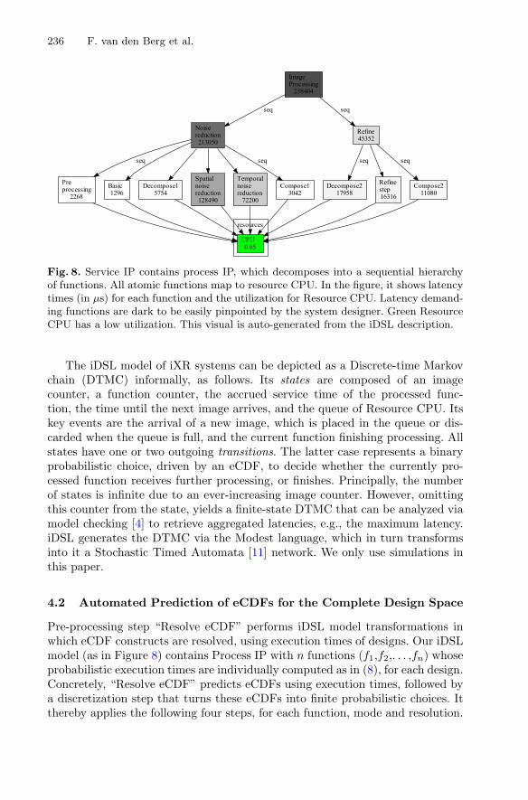
The iDSL model is defined as follows. Process Image Processing (IP) encom-passes two high-level functions “Noise reduction” and “Refine”, which in turndecompose into a sequence of n atomic functions f1,f2,. . . ,fn (as depicted inFigure 8). IP is enclosed by a Mutual Exclusion to enforce a strict FIFO schedul-ing policy by processing images in one go. The only resource, CPU, is equippedwith a FIFO queue. Service IP maps all processes to the CPU. The Scenarioprescribes that images arrive f times per second with fixed inter-arrival times,where f is the frame-rate. The Measure simulation yields, in one run, latenciesof 50 images and the utilization of the CPU. The Design space is the Cartesianproduct resolution and mode. However, to compute two trade-off graphs (as inFigure 9), we also vary the buffer size and frame-rate.

Fig. 7. The concepts of iDSL [4]: Aservice system provides services toconsumers. A service is implementedusing a process, resource and map-ping. A process decomposes servicerequests into atomic tasks, each assignedto resources by the mapping. Resourcesperform one atomic task at a time. A sce-nario comprises invoked service requestsover time. A study evaluates a set sce-narios to derive the system’s charac-teristics. Measures of interest are theretrieved measures.


Fig. 8. Service IP contains process IP, which decomposes into a sequential hierarchyof functions. All atomic functions map to resource CPU. In the figure, it shows latencytimes (in μs) for each function and the utilization for Resource CPU. Latency demand-ing functions are dark to be easily pinpointed by the system designer. Green ResourceCPU has a low utilization. This visual is auto-generated from the iDSL description.

The iDSL model of iXR systems can be depicted as a Discrete-time Markovchain (DTMC) informally, as follows. Its states are composed of an imagecounter, a function counter, the accrued service time of the processed func-tion, the time until the next image arrives, and the queue of Resource CPU. Itskey events are the arrival of a new image, which is placed in the queue or dis-carded when the queue is full, and the current function finishing processing. Allstates have one or two outgoing transitions. The latter case represents a binaryprobabilistic choice, driven by an eCDF, to decide whether the currently pro-cessed function receives further processing, or finishes. Principally, the numberof states is infinite due to an ever-increasing image counter. However, omittingthis counter from the state, yields a finite-state DTMC that can be analyzed viamodel checking [4] to retrieve aggregated latencies, e.g., the maximum latency.iDSL generates the DTMC via the Modest language, which in turn transformsinto it a Stochastic Timed Automata [11] network. We only use simulations inthis paper.

4.2 Automated Prediction of eCDFs for the Complete Design Space

Pre-processing step “Resolve eCDF” performs iDSL model transformations inwhich eCDF constructs are resolved, using execution times of designs. Our iDSLmodel (as in Figure 8) contains Process IP with n functions (f1,f2,. . . ,fn) whoseprobabilistic execution times are individually computed as in (8), for each design.Concretely, “Resolve eCDF” predicts eCDFs using execution times, followed bya discretization step that turns these eCDFs into finite probabilistic choices. Itthereby applies the following four steps, for each function, mode and resolution.


First, the required eCDFs, as in the right hand of (8), are obtained by retriev-ing the corresponding execution times, from which in turn eCDFs are estimated.Second, solving this equation yields the eCDF to be predicted. Third, n samplesare taken from this predicted eCDF for probabilities ( 1

n , 2n ,· · · ,1) to discretize it,i.e., we use n = 1000. Fourth, these n samples are combined in a probabilisticchoice, a process algebra construct that iDSL supports by default. After this,the resulting probabilistic choices are ordered by design and function within thatdesign, and added to the iDSL model.

4.3 Automated Aggregation of Latencies

The post-processing step “Compute aggregate” applies, for each design, a num-ber of aggregate functions on n obtained latencies from simulations (we usen = 50). We selected the average, maximum and median as the functions ofinterest (for an example, see Table 1). Concretely, “Compute aggregate” executeswhen a simulation run finishes and computes the specified aggregate functions.

Next, “Process aggregate values” generates trade-off plots [6,9] that help thesystem designer with balancing between two system aspects by plotting theseaspects of designs in a 2D-plane (for examples, see Figure 9). They visualize howgains on one system aspect pay its toll on another. A design dominates anotherdesign when it ranks better on one aspect and is at least a good on the otheraspect. Dominated designs are called Pareto suboptimal, others Pareto optimal.

Finally, “Process aggregate values” sorts design instances on each individualaspect. This enables the comparison of designs on a particular system aspect.

5 Results of a Case Study on iXR Systems

In this section, we study the performance results of an iXR system to show thevalidity and applicability of our work by evaluating a concrete iXR system.

We obtained all results by executing the constructed iDSL model on aPC (AMD A6-3400M, 8Gb RAM) using 32’27” (minutes, seconds). PredictingeCDFs took 1’48” (6%), simulations 30’13” (91%) and aggregate functions 19”(1%).

5.1 The Performance of an iXR System

In the following, we present eCDFs with execution times and correspondingaggregate metrics, a latency break-down graph, and two trade-off graphs.

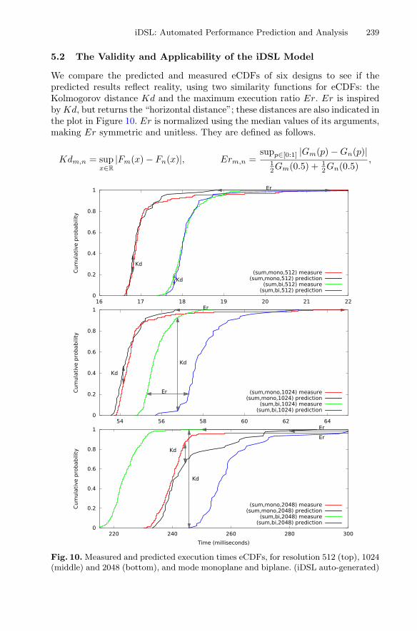
We assess if the performance of biplane iXR systems on shared hardware isas good as monoplane ones. We use eCDFs with execution times in whichwe compare the measured performance (in Figure 10) of these biplane systems(green) with monoplane ones (red), for resolutions 5122 (top), 10242 (middle)and 20482 (bottom). As an effect of sharing hardware, biplane systems performworse than monoplane ones for image resolutions 5122 and 10242, viz., theiraverage latencies are 6% and 2% higher (as in Table 1), respectively. In contrast,


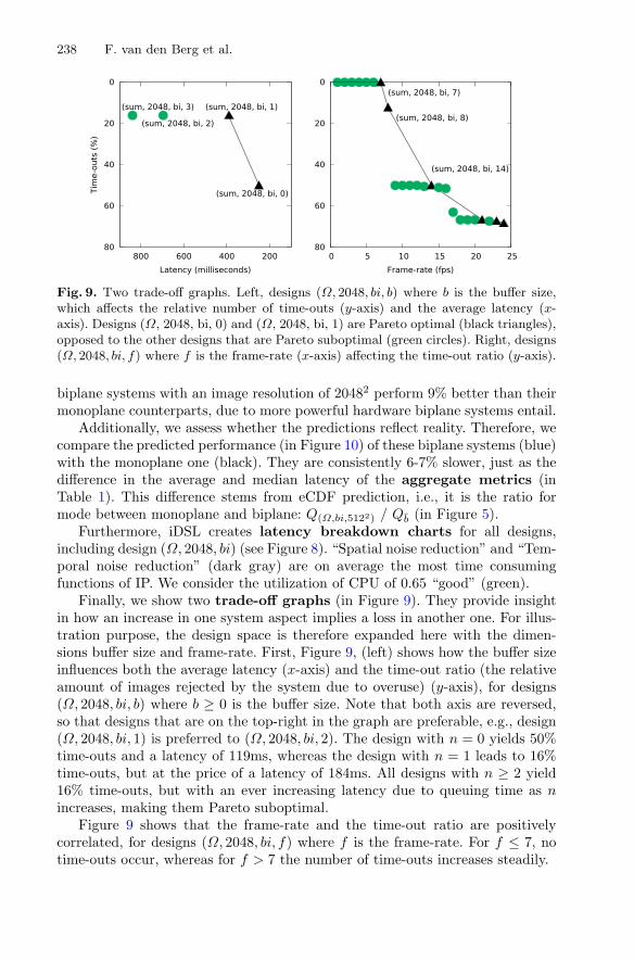
Fig. 9. Two trade-off graphs. Left, designs (Ω, 2048, bi, b) where b is the buffer size,which affects the relative number of time-outs (y-axis) and the average latency (x-axis). Designs (Ω, 2048, bi, 0) and (Ω, 2048, bi, 1) are Pareto optimal (black triangles),opposed to the other designs that are Pareto suboptimal (green circles). Right, designs(Ω, 2048, bi, f) where f is the frame-rate (x-axis) affecting the time-out ratio (y-axis).

biplane systems with an image resolution of 20482 perform 9% better than theirmonoplane counterparts, due to more powerful hardware biplane systems entail.

Additionally, we assess whether the predictions reflect reality. Therefore, wecompare the predicted performance (in Figure 10) of these biplane systems (blue)with the monoplane one (black). They are consistently 6-7% slower, just as thedifference in the average and median latency of the aggregate metrics (inTable 1). This difference stems from eCDF prediction, i.e., it is the ratio formode between monoplane and biplane: Q(Ω,bi,5122) / Qb (in Figure 5).

Furthermore, iDSL creates latency breakdown charts for all designs,including design (Ω, 2048, bi) (see Figure 8). “Spatial noise reduction” and “Tem-poral noise reduction” (dark gray) are on average the most time consumingfunctions of IP. We consider the utilization of CPU of 0.65 “good” (green).

Finally, we show two trade-off graphs (in Figure 9). They provide insightin how an increase in one system aspect implies a loss in another one. For illus-tration purpose, the design space is therefore expanded here with the dimen-sions buffer size and frame-rate. First, Figure 9, (left) shows how the buffer sizeinfluences both the average latency (x-axis) and the time-out ratio (the relativeamount of images rejected by the system due to overuse) (y-axis), for designs(Ω, 2048, bi, b) where b ≥ 0 is the buffer size. Note that both axis are reversed,so that designs that are on the top-right in the graph are preferable, e.g., design(Ω, 2048, bi, 1) is preferred to (Ω, 2048, bi, 2). The design with n = 0 yields 50%time-outs and a latency of 119ms, whereas the design with n = 1 leads to 16%time-outs, but at the price of a latency of 184ms. All designs with n ≥ 2 yield16% time-outs, but with an ever increasing latency due to queuing time as nincreases, making them Pareto suboptimal.

Figure 9 shows that the frame-rate and the time-out ratio are positivelycorrelated, for designs (Ω, 2048, bi, f) where f is the frame-rate. For f ≤ 7, notime-outs occur, whereas for f > 7 the number of time-outs increases steadily.


5.2 The Validity and Applicability of the iDSL Model

We compare the predicted and measured eCDFs of six designs to see if thepredicted results reflect reality, using two similarity functions for eCDFs: theKolmogorov distance Kd and the maximum execution ratio Er. Er is inspiredby Kd, but returns the “horizontal distance”; these distances are also indicated inthe plot in Figure 10. Er is normalized using the median values of its arguments,making Er symmetric and unitless. They are defined as follows.

Kdm,n = supx∈R

|Fm(x) − Fn(x)|, Erm,n =supp∈[0:1] |Gm(p) − Gn(p)|

12Gm(0.5) + 1

2Gn(0.5),

Fig. 10. Measured and predicted execution times eCDFs, for resolution 512 (top), 1024(middle) and 2048 (bottom), and mode monoplane and biplane. (iDSL auto-generated)


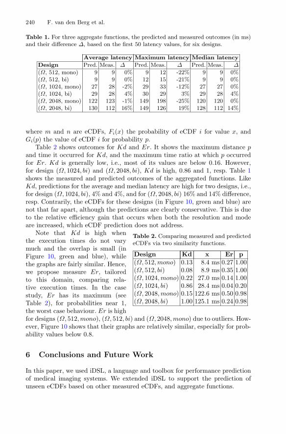
Table 1. For three aggregate functions, the predicted and measured outcomes (in ms)and their difference Δ, based on the first 50 latency values, for six designs.

Average latency Maximum latency Median latency

Design Pred. Meas. Δ Pred. Meas. Δ Pred. Meas. Δ

(Ω, 512, mono) 9 9 0% 9 12 -22% 9 9 0%(Ω, 512, bi) 9 9 0% 12 15 -21% 9 9 0%(Ω, 1024, mono) 27 28 -2% 29 33 -12% 27 27 0%(Ω, 1024, bi) 29 28 4% 30 29 3% 29 28 4%(Ω, 2048, mono) 122 123 -1% 149 198 -25% 120 120 0%(Ω, 2048, bi) 130 112 16% 149 126 19% 128 112 14%

where m and n are eCDFs, Fi(x) the probability of eCDF i for value x, andGi(p) the value of eCDF i for probability p.

Table 2 shows outcomes for Kd and Er. It shows the maximum distance pand time it occurred for Kd, and the maximum time ratio at which p occurredfor Er. Kd is generally low, i.e., most of its values are below 0.16. However,for design (Ω, 1024, bi) and (Ω, 2048, bi), Kd is high, 0.86 and 1, resp. Table 1shows the measured and predicted outcomes of the aggregated functions. LikeKd, predictions for the average and median latency are high for two designs, i.e.,for design (Ω, 1024, bi), 4% and 4%, and for (Ω, 2048, bi) 16% and 14% difference,resp. Contrarily, the eCDFs for these designs (in Figure 10, green and blue) arenot that far apart, although the predictions are clearly conservative. This is dueto the relative efficiency gain that occurs when both the resolution and modeare increased, which eCDF prediction does not address.

Table 2. Comparing measured and predictedeCDFs via two similarity functions.

Design Kd x Er p(Ω, 512,mono) 0.13 8.4 ms 0.27 1.00(Ω, 512, bi) 0.08 8.9 ms 0.35 1.00(Ω, 1024,mono) 0.22 27.0 ms 0.14 1.00(Ω, 1024, bi) 0.86 28.4 ms 0.04 0.20(Ω, 2048,mono) 0.15 122.6 ms 0.50 0.98(Ω, 2048, bi) 1.00 125.1 ms 0.24 0.98

Note that Kd is high whenthe execution times do not varymuch and the overlap is small (inFigure 10, green and blue), whilethe graphs are fairly similar. Hence,we propose measure Er, tailoredto this domain, comparing rela-tive execution times. In the casestudy, Er has its maximum (seeTable 2), for probabilities near 1,the worst case behaviour. Er is highfor designs (Ω, 512,mono), (Ω, 512, bi) and (Ω, 2048,mono) due to outliers. How-ever, Figure 10 shows that their graphs are relatively similar, especially for prob-ability values below 0.8.

6 Conclusions and Future Work

In this paper, we used iDSL, a language and toolbox for performance predictionof medical imaging systems. We extended iDSL to support the prediction ofunseen eCDFs based on other measured eCDFs, and aggregate functions.


iDSL provides a performance evaluation approach in which we (i) rely on fewcostly measurements; (ii) use the iDSL toolset to automatically evaluate manydesigns and present the results visually; (iii) automatically generate aggregatedmetrics; and (iv) evaluate the performance of complex iXR systems.

In a case study, we have investigated the performance effect of biplane iXRsystems on shared hardware. Measurements indicate that these systems performas good as monoplane ones, but predictions show more conservative results.

iDSL generates latency breakdown charts for each design that show the sys-tem designer the process structure, the time consuming processes and resourceutilizations, at one glance. iDSL also generates trade-off graphs, in which designsare plotted on two oppose system aspects. They provide the system designerinsight in how an increase on one system aspect implies a loss on another one.

We validated the model by comparing its outcomes with measurements. Theymostly reflect reality, but are conservative for high resolution biplane systems.The case study involved a medical imaging system, but we consider the approachapplicable to many service-oriented systems.

In parallel work we have extended iDSL with probabilistic model checkingto obtain execution time eCDFs [3] using the Modest toolset [11].

Acknowledgements. We would like to thank Arnd Hartmanns of the Modest team at

Saarland University for his efforts made during the development of iDSL, and Mathijs

Visser at Philips Healthcare for giving us insight in the iXR system case study and for

performing measurements.

References

1. Ayer, M., Brunk, D., Ewing, G., Reid, W., Silverman, E.: An empirical distributionfunction for sampling with incomplete information. The Annals of MathematicalStatistics 26(4), 641–647 (1955)

2. Basten, T., van Benthum, E., Geilen, M., Hendriks, M., Houben, F., Igna,G., Reckers, F., de Smet, S., et al.: Model-driven design-space exploration forembedded systems: the octopus toolset. In: Margaria, T., Steffen, B. (eds.) ISoLA2010, Part I. LNCS, vol. 6415, pp. 90–105. Springer, Heidelberg (2010)

3. van den Berg, F., Hooman, J., Hartmanns, A., Haverkort, B., Remke, A.:Computing response time distributions using iterative probablistic model check-ing. In: Computer Performance Engineering, LNCS, vol. 9272. Springer (2015) (toappear)

4. van den Berg, F., Remke, A., Haverkort, B.R.: A domain specific language forperformance evaluation of medical imaging systems. In: 5th Workshop on MedicalCyber-Physical Systems, pp. 80–93. Schloss Dagstuhl (2014)

5. van den Berg, F., Remke, A., Mooij, A., Haverkort, B.: Performance evaluationfor collision prevention based on a domain specific language. In: Balsamo, M.S.,Knottenbelt, W.J., Marin, A. (eds.) EPEW 2013. LNCS, vol. 8168, pp. 276–287.Springer, Heidelberg (2013)

6. Censor, Y.: Pareto optimality in multiobjective problems. Applied Mathematicsand Optimization 4(1), 41–59 (1977)

7. Conway, R.: Some tactical problems in digital simulation. Management Science10(1), 47–61 (1963)


8. Devroye, L.: Sample-based non-uniform random variate generation. In: Proceedingsof the 18th Winter simulation conference, pp. 260–265. ACM (1986)

9. Ghodsi, R., Skandari, M., Allahverdiloo, M., Iranmanesh, S.: A new practical modelto trade-off time, cost, and quality of a project. Australian Journal of Basic andApplied Sciences 3(4), 3741–3756 (2009)

10. Groote, J., Osaiweran, A., Wesselius, J.: Analyzing the effects of formal methodson the development of industrial control software. In: 27th IEEE InternationalConference on Software Maintenance, pp. 467–472. IEEE (2011)

11. Hartmanns, A., Hermanns, H.: The modest toolset: an integrated environmentfor quantitative modelling and verification. In: Abraham, E., Havelund, K. (eds.)TACAS 2014 (ETAPS). LNCS, vol. 8413, pp. 593–598. Springer, Heidelberg (2014)

12. Haveman, S., Bonnema, G., van den Berg, F.: Early insight in systems designthrough modeling and simulation. Procedia Computer Science 28, 171–178 (2014)

13. Igna, G., Vaandrager, F.: Verification of printer datapaths using timed automata.In: Margaria, T., Steffen, B. (eds.) ISoLA 2010, Part II. LNCS, vol. 6416,pp. 412–423. Springer, Heidelberg (2010)

14. Johnson, J.: Designing with the Mind in Mind: Simple Guide to UnderstandingUser Interface Design Rules. Morgan Kaufmann (2010)

15. Wilson, J.: Gantt charts: A centenary appreciation. European Journal ofOperational Research 149(2), 430–437 (2003)

idsl: automated performance prediction and analysis of ... · viz., image processing of ixr...

Documents