ieee transactions 1 optimal inversion of the anscombe...

IEEE TRANSACTIONS 1

Optimal inversion of the Anscombe transformationin low-count Poisson image denoising

Markku Mäkitalo and Alessandro Foi

Abstract�The removal of Poisson noise is often performedthrough the following three-step procedure. First, the noise vari-ance is stabilized by applying the Anscombe root transformationto the data, producing a signal in which the noise can be treatedas additive Gaussian with unitary variance. Second, the noise isremoved using a conventional denoising algorithm for additivewhite Gaussian noise. Third, an inverse transformation is appliedto the denoised signal, obtaining the estimate of the signal ofinterest.The choice of the proper inverse transformation is crucial in

order to minimize the bias error which arises when the nonlinearforward transformation is applied. We introduce optimal inversesfor the Anscombe transformation, in particular the exact unbi-ased inverse, a maximum likelihood (ML) inverse, and a moresophisticated minimum mean square error (MMSE) inverse. Wethen present an experimental analysis using a few state-of-the-art denoising algorithms and show that the estimation can beconsistently improved by applying the exact unbiased inverse,particularly at the low-count regime. This results in a veryef�cient �ltering solution that is competitive with some of thebest existing methods for Poisson image denoising.

Index Terms�denoising, photon-limited imaging, Poissonnoise, variance stabilization.

I. INTRODUCTION

Poisson noise is characteristic of many image acquisitionmodalities, and its removal is of fundamental importance formany applications and particularly in astronomy and medicalimaging. As the noise variance equals the expected value ofthe underlying true signal, Poisson noise is signal dependent,which makes the premise for Poisson denoising very differentfrom the case of additive white Gaussian noise with constantvariance typically assumed by signal processing �lters.Although denoising algorithms speci�cally designed for

Poisson noise have been proposed (e.g., [1], [2], [3], [4], [5],[6], [7]), often the removal of Poisson noise is performedthrough the following three-step procedure. First, the noisevariance is stabilized by applying the Anscombe root trans-formation [8] f : z 7�! 2

qz C 3

8 to the data. This produces asignal in which the noise can be treated as additive Gaussianwith unitary variance. Second, the noise is removed using aconventional denoising algorithm for additive white Gaussiannoise. Third, an inverse transformation is applied to thedenoised signal, obtaining the estimate of the signal of interest.This paper focuses on this last step and aims at identifying

and emphasizing the role that the inversion plays in ensuringthe success of the whole procedure.

This work was supported by the Academy of Finland (project no. 213462,Finnish Programme for Centres of Excellence in Research 2006-2011, projectno. 118312, Finland Distinguished Professor Programme 2007-2010, andproject no. 129118, Postdoctoral Researcher's Project 2009-2011).

In the recent years, variance stabilization has often beenquestioned as a viable method for Poisson noise removalbecause of the poor numerical results achieved at the low-count regime, i.e. for low-intensity signals, which correspondsto the case of low signal-to-noise ratio (SNR). We showthat this disappointing performance, reported in many earlierworks (e.g., [1], [2], [3]), is not due to the stabilization itself(i.e. to the forward transformation), but rather to the inversetransformation.The choice of the proper inverse transformation is crucial

in order to minimize the bias error which arises when thenonlinear forward transformation is applied. Both the algebraicinverse and the asymptotically unbiased inverse proposedby Anscombe [8] lead to a signi�cant bias at low counts.In particular, the latter inverse provides unbiasedness onlyasymptotically for large counts while at low counts it leadsto a larger bias than the former one.This work extends our preliminary paper [9] by considering

more general optimal inverses for the Anscombe transforma-tion. First we introduce the exact unbiased inverse and showthat it coincides with a form of maximum likelihood (ML)inverse, and then we consider a more sophisticated minimummean square error (MMSE) inverse. After that, we presentan extensive experimental analysis using a few state-of-the-art denoising algorithms and show that the results can beconsistently improved by applying the exact unbiased inverse.In particular, the combination of BM3D [10] and the exactunbiased inverse outperforms some of the best existing algo-rithms speci�cally targeted at Poisson noise removal, whilemaintaining low computational complexity.The rest of the paper is organized as follows: Section II

introduces some preliminaries about Poisson noise, variancestabilization and the conventional inverses of the Anscombetransformation. In Section III we consider optimal inversetransformations: �rst we propose the exact unbiased inverse,which can be interpreted as a maximum likelihood inverse,and �nally we discuss the minimum mean square error in-verse. Section IV consists of various experiments, followedby discussion and conclusions in Section V.

II. PRELIMINARIES

A. Poisson noise

Let zi ; i D 1; : : : ; N , be the observed pixel values obtainedthrough an image acquisition device. We consider each zi to bean independent random Poisson variable whose mean yi � 0is the underlying intensity value to be estimated. Explicitly,

2 IEEE TRANSACTIONS

the discrete Poisson probability of each zi is

P .zi j yi / Dyzii e

�yi

zi !: (1)

In addition to being the mean of the Poisson variable zi , theparameter yi is also its variance:

Efzi j yi g D yi D varfzi j yi g: (2)Poisson noise can be formally de�ned as

�i D zi � Efzi j yi g; (3)thus, we trivially have Ef�i j yi g D 0 and varf�i j yi g Dvarfzi j yi g D yi . Since the noise variance depends onthe true intensity value, Poisson noise is signal dependent.More speci�cally, the standard deviation of the noise �iequals pyi . Due to this, the effect of Poisson noise increases(i.e. the signal-to-noise ratio decreases) as the intensity valuedecreases.

B. Variance stabilization and the Anscombe transformationThe rationale behind applying a variance-stabilizing trans-

formation is to remove the data-dependence of the noisevariance, so that it becomes constant throughout the wholedata zi , i D 1; : : : ; N . Moreover, if the transformation is alsonormalizing (i.e. it results in a Gaussian noise distribution),we can estimate the intensity values yi with a conventionaldenoising method designed for additive white Gaussian noise.Neither exact stabilization nor exact normalization are possible[11], [12], therefore, in practice, approximate or asymptoticalresults are employed.One of the most popular variance-stabilizing transforma-

tions is the Anscombe transformation [8]

f .z/ D 2rz C

38: (4)

Applying (4) to Poisson distributed data gives a signal whosenoise is asymptotically additive standard normal.The denoising of f .z/ produces a signal D that can be

considered as an estimate of Ef f .z/ j yg. We need to applyan inverse transformation to D in order to obtain the desiredestimate of y. The direct algebraic inverse of (4) is

IA.D/ D f �1.D/ D�D2

�2�38; (5)

but the resulting estimate of y is biased, because the nonlin-earity of the transformation f means we generally have

Ef f .z/ j yg 6D f .Efz j yg/; (6)and, thus,

f �1.Ef f .z/ j yg/ 6D Efz j yg: (7)

Another possibility is to use the adjusted inverse [8]

IB.D/ D�D2

�2�18; (8)

which provides asymptotical unbiasedness for large counts.This is the inverse typically used in applications.

III. OPTIMAL INVERSE TRANSFORMATIONSWhile the asymptotically unbiased inverse (8) provides good

results for high-count data, applying it to low-count data leads

to a biased estimate, as can be seen, e.g., in [1]. Here weconsider three types of optimal inverses.

A. Exact unbiased inverseProvided a successful denoising, i.e. D is treated as

Ef f .z/ j yg, the exact unbiased inverse of the Anscombetransformation f is an inverse transformation IC that mapsthe values Ef f .z/ j yg to the desired values Efz j yg:

IC : Ef f .z/ j yg 7�! Efz j yg: (9)Since Efz j yg D y for any given y, the problem of �ndingthe inverse IC reduces to computing the values Ef f .z/ j yg,which is done by numerical evaluation of the integral corre-sponding to the expectation operator E :

Ef f .z/ j yg DZ C1

�1f .z/p.z j y/ dz; (10)

where p.z j y/ is the generalized probability density functionof z conditioned on y. In our case we have discrete Poissonprobabilities P .z j y/, so we can replace the integral bysummation:

Ef f .z/ j yg DC1XzD0

f .z/P.z j y/: (11)

Further, since here f .z/ is the forward Anscombe transforma-tion (4), we can write (11) as

Ef f .z/ j yg D 2C1XzD0

rz C

38�yze�y

z!

!: (12)

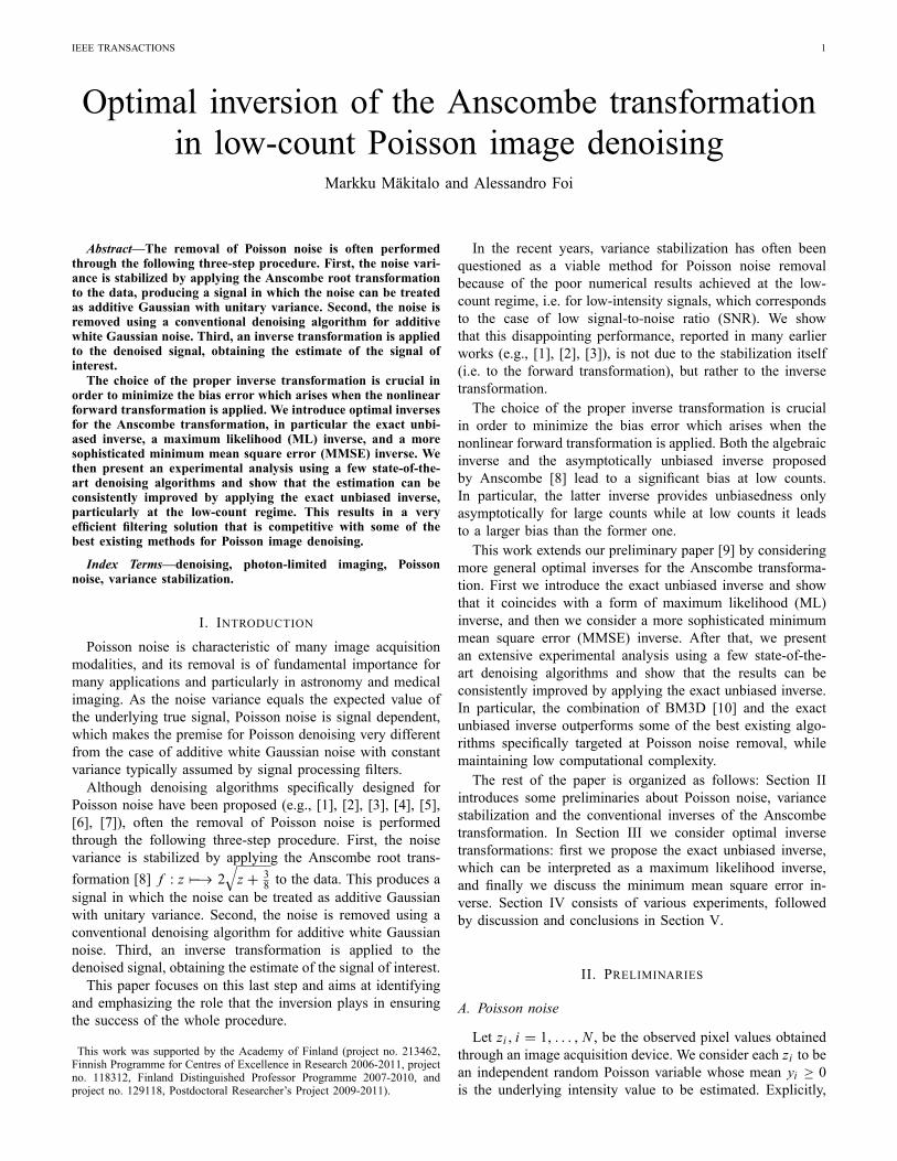
Figure 1 shows the plots of the inverse transformations IA,IB and IC . Since IC is unbiased, we see that at low countsthe asymptotically unbiased inverse actually leads to a largerbias than the algebraic inverse.Let us remark that if the exact unbiased inverse (9) is applied

to the denoised data D with some errors (in the sense thatD 6D Ef f .z/jyg), then the estimation error in Oy D IC .D/ caninclude variance as well as bias components. In general, theunbiasedness of IC holds only provided that D D Ef f .z/jygexactly, as it is assumed when de�ning (9).

B. ML inverseIn the previous Section III-A we assumed that the denoising

is successful (i.e. we can treat the denoised signal D asEf f .z/ j yg), which then lead us to the concept of the exactunbiased inverse. Now we consider a more general scenario,where this assumption does not necessarily hold: instead ofthe strict equality, we assume that the pointwise mean squareerror of D as an estimate of Ef f .z/ j yg is

"2 D En.D � Ef f .z/ j yg/2

o: (13)

In practice the distribution of D is unknown. For simplicity,we assume that D is normally distributed around Ef f .z/ j ygwith variance "2:

D � N�Ef f .z/ j yg; "2

�: (14)

While formally (14) implies that D is an unbiased estimate ofEf f .z/ j yg, in fact also unknown estimation-bias errors canbe considered as contributors of "2, with the symmetry of the

MÄKITALO AND FOI, OPTIMAL INVERSION OF THE ANSCOMBE TRANSFORMATION IN LOW-COUNT POISSON IMAGE DENOISING 3

distribution about Ef f .z/ j yg re�ecting our uncertainty aboutthe sign of the bias.By treating D as the data, the maximum likelihood (ML)

inverse is de�ned asIML.D/ D argmax

yp.D j y/; (15)

where, according to (14),

p.D j y/ D1

p2�"2

e�12"2.D�Ef f .z/jyg/2

: (16)

Under the above assumptions, this equals to (see Appendixfor details)

IML.D/ D�IC .D/, if D � 2

p3=8

0, if D < 2p3=8: (17)

Thus, the exact unbiased inverse coincides with this form ofML inverse. Note also that IML.D/ is independent of ". Theobtained result (17) holds for any unimodal distribution whosemode is Ef f .z/ j yg.

C. MMSE inverseUnder the same hypotheses of Section III-B, we de�ne

the minimum mean square error (MMSE) inverse, which isparametrized by ", asIMMSE.D; "/ D argmin

OyEf.y � Oy/2 j Dg

D argminOy

Z C1

�1p.y j D/

�y � Oy

�2 dy: (18)

It is worth reminding that we assume D to be normallydistributed according to (14); if this assumption does not hold,the obtained inverse is not necessarily the true minimum MSEinverse.Additionally assuming that the true signal y is uniformly

distributed, solving for Oy (see Appendix for details) producesthe following formula for computing the inverse:

Oy DR C10 p.D j y/y dyR C10 p.D j y/ dy

; (19)

where p .D j y/ is given by (16). Note that the exact unbiasedinverse can be considered a limit case of the MMSE inverse,obtained when " D 0, because p .D j y/ becomes a Diracimpulse centered at that particular value of y such thatEf f .z/ j yg D D. In other words,

IMMSE.D; 0/ D IC .D/ D IML.D/: (20)Figure 2 shows the MMSE inverse transformations for somevalues of ", including the case " D 0.

IV. EXPERIMENTSAll of our experiments consist of the same three-step

denoising procedure: First we apply the forward Anscombetransformation (4) to a noisy image. Then we denoise thetransformed image (assuming additive white Gaussian noiseof unit variance) with either BM3D [10], SAFIR [13] or BLS-GSM [14], and �nally we apply an inverse transformation inorder to get the �nal estimate. We do not provide comparisonsagainst the Haar-Fisz algorithm [4] or platelets [6], [7], as boththe MS-VST [1] and PURE-LET [3] algorithms have been

1.4 1.6 1.8 2 2.2 2.4 2.6 2.8 30

0.2

0.4

0.6

0.8

1

1.2

1.4

1.6

1.8

2

Fig. 1. Inverse Anscombe transformations IA (algebraic), IB (asymptoticallyunbiased) and IC (exact unbiased). For the exact unbiased inverse, Dcoincides with Ef f .z/ j yg, hence its bias is zero.

1 0 1 2 3 4

0

0.5

1

1.5

2

2.5

3

3.5

4

ε = 0

ε = 0.07

ε = 0.18

ε = 0.40

ε = 0.71

ε = 1

ε = 1.33

ε = 1.72

Fig. 2. MMSE inverse transformations (18) for some values of ". The case" D 0 corresponds to the exact unbiased inverse transformation (9) and theML inverse transformation (17).

shown to outperform them, and we further compare these twoalgorithms against ours.To implement the exact unbiased inverse IC in practice, it

is suf�cient to compute (12) for a limited set of values y; forarbitrary values of y we then use linear interpolation basedon these computed values of (12), and for large values1 ofy we approximate IC by IB . In similar fashion, the MMSEinverse can be obtained based on numerical evaluation of thetwo integrals in (19).Matlab functions implementing these two optimal

inverse transformations are available online athttp://www.cs.tut.�/~foi/invansc.We evaluate the performance either by normalized mean

integrated square error (NMISE) or by peak signal-to-noise

1In our implementation, we consider y to be large if y > 2500.

4 IEEE TRANSACTIONS

ratio (PSNR). The NMISE is calculated using the formula1NN

Xi :yi>0

�. Oyi � yi /2=yi

�; (21)

where Oyi are the estimated intensities, yi the respective truevalues, and the sum is computed over the NN pixels in theimage for which yi > 0. The PSNR is calculated using theformula

10 log10

0@ maxi .yi /2�Pi�Oyi � yi

�2=N�1A ; (22)

where N is the total number of pixels in the image.In Section IV-A we consider the exact unbiased inverse, and

Section IV-B consists of experiments with the MMSE inverse.Section IV-C addresses the computational complexity of theinverse transformations and the denoising algorithms.

A. Exact unbiased inverseWe consider three sets of experiments in order to compare

against the three recent works [1], [2] and [3], each ofwhich proposes an algorithm speci�cally designed for Poissonnoise removal (MS-VST, PH-HMT and Interscale PURE-LET,respectively).1) NMISE comparison against MS-VST [1] and PH-HMT

[2]: For the �rst set we proceed in the same way as in [1]in order to produce comparable results: The above-mentionedthree-step denoising procedure is performed �ve times for eachimage, each time with a different realization of the randomnoise. We evaluate the performance by using NMISE, and theobtained NMISE values are �nally averaged over these �vereplications. This metric was chosen because of the availableresults for comparison in [1] and [2]. The authors of [1] alsokindly provided us with their set of test images (all of them256�256 in size), shown in Figure 3.The denoising is done with either BM3D, SAFIR or BLS-

GSM, and for the inversion of the denoised signal we use theexact unbiased inverse. The same experiments are also donefor the asymptotically unbiased inverse (8), whose results serveas a point of comparison.The numerical results of our experiments are presented in

Table I, where we also compare them to the state-of-the-artresults obtained with the PH-HMT and MS-VST algorithmsproposed in [2] and [1], respectively. In addition, we haveincluded the results obtained in [1] with the asymptoticallyunbiased inverse Anscombe transformation combined withvarious undecimated wavelet transforms (here collectivelydenoted as WT). Table I shows not only that the exact unbiasedinverse produces signi�cantly better results at low counts thanthe asymptotically unbiased inverse, but also that the methodis competitive with both PH-HMT and MS-VST. In particular,the combination of BM3D and the exact unbiased inverseoutperforms both of them in terms of NMISE.Figures 4�5 illustrate the improvement that is achieved

(especially at low counts) by applying the exact unbiasedinverse instead of the asymptotically unbiased inverse, whileFigure 6 compares the different algorithms for the denoisingof the Cells image (the exact unbiased inverse combined with

BM3D, SAFIR and BLS-GSM, and the best MS-VST resultfrom [1]). In addition, we present a chosen cross-section (i.e.one row) of some of the test images in Figure 7. Theseplots also clearly demonstrate that at low counts the exactunbiased inverse provides a signi�cant improvement over theasymptotically unbiased inverse, whereas at high counts thedifference is expectedly negligible.For additional �gures we refer to our preliminary paper [9].2) PSNR comparison against PH-HMT [2]: In the second

part of the experiments we use the test images shown inFigure 8 and evaluate the performance in terms of PSNR,thus enabling us to compare against the PH-HMT results in[2]. This time we scale each image to seven different peakintensity levels (1, 2, 3, 4, 5, 10 and 20), and for each ofthem we perform the denoising procedure ten times, with tendifferent realizations of the random noise.As above, we use either BM3D, SAFIR or BLS-GSM for

the denoising, and the inversion is done with either the exactunbiased inverse or the asymptotically unbiased inverse.The results, which are averages of ten PSNR values, are

reported in Table II. We see again that at low peak intensitieswe get a substantial improvement by applying the exact un-biased inverse instead of the asymptotically unbiased inverse,regardless of the used denoising algorithm. Indeed, the bestresults of the table mainly correspond to algorithms combinedwith the exact unbiased inverse. In particular, the best overallperformance is obtained with BM3D, although both SAFIRand PH-HMT provide competitive results especially at thelowest peak intensities. The different performance at lowcounts is possibly explained by SAFIR exploiting adaptivewindow sizes, as opposed to BM3D, which uses �xed-sizeblocks.Note that the average PSNR values of the noisy images in

Table II have minor differences to those reported in [2] dueto different realizations of the random noise.3) PSNR comparison against PURE-LET [3]: The third

part of our experiments is very similar to the second one,with the following differences: Now we use the four testimages shown in Figure 9 and compare our results against thebest results obtained with the Interscale PURE-LET (with twocyclic shifts) [3]. Each image is scaled to the peak intensitylevels 1, 5, 10, 20, 30, 60 and 120, so we do not focus at lowcounts as much as earlier.As in [3], the denoising performance is evaluated in terms

of PSNR. Table III presents the obtained results (averages often values), which are consistent with the results in Table II:the overall performance of BM3D is strong, but it is oftenoutperformed by SAFIR at the lower peak intensity levels.It is interesting to note that for an image like Moon, whichpresents a large black background area that is completely�at, the performance gap between multiscale (BLS-GSM andPURE-LET) and patch-based (BM3D and SAFIR) methods isreduced, in as much as in a few cases the former methods areproducing slightly better numerical results than the latter ones.4) Summary: All three sets of experiments produce consis-

tent results, showing that at low intensities we obtain signif-icantly better results by applying the exact unbiased inverseinstead of the asymptotically unbiased inverse, whereas at high


Spots (256�256) Galaxy (256�256) Ridges (256�256) Barbara (256�256) Cells (256�256)Fig. 3. The �ve test images used in the experiments of Sections IV-A1 and IV-B.

TABLE IAVERAGE NMISE VALUES FOR THE ASYMPTOTICALLY UNBIASED INVERSE AND THE EXACT UNBIASED INVERSE, AND A COMPARISON TO THE RESULTSOBTAINED IN [2] AND [1] WITH ALGORITHMS SPECIFICALLY DESIGNED FOR POISSON NOISE REMOVAL. THE INTENSITY RANGE OF EACH IMAGE IS

INDICATED IN BRACKETS.

Asymptotically unbiased inverse Exact unbiased inverse Other algorithmsWT [1] BM3D SAFIR BLS-GSM BM3D SAFIR BLS-GSM PH-HMT [2] MS-VST [1]

Spots [0.03, 5.02] 2.34 1.7424 1.7495 2.0370 0.0365 0.0384 0.1871 0.048 0.069Galaxy [0, 5] 0.15 0.1026 0.1110 0.1253 0.0299 0.0301 0.0385 0.030 0.035Ridges [0.05, 0.85] 0.83 0.7025 0.7252 0.7694 0.0128 0.0173 0.0331 - 0.017Barbara [0.93, 15.73] 0.26 0.0881 0.1178 0.1122 0.0881 0.1178 0.1123 0.159 0.17Cells [0.53, 16.93] 0.095 0.0660 0.0683 0.0718 0.0649 0.0671 0.0707 0.082 0.078

(a) (b) (c) (d) (e)

Fig. 4. (a) Original Spots image (intensity range [0.03, 5.02]), (b) Poisson-count image, (c) image denoised with BM3D and the asymptotically unbiasedinverse (average NMISE = 1.7395), (d) image denoised with BM3D and the exact unbiased inverse (average NMISE = 0.0365), (e) image denoised withSAFIR and the exact unbiased inverse (average NMISE = 0.0384). The images shown here are gamma-corrected ( D 0:6) for improved visibility of thedarker areas. A cross-section of images (a), (c) and (d) is shown in Figure 7(a).

(a) (b) (c) (d) (e)

Fig. 5. (a) Original Galaxy image (intensity range [0, 5]), (b) Poisson-count image, (c) image denoised with BM3D and the asymptotically unbiased inverse(average NMISE = 0.1025), (d) image denoised with BM3D and the exact unbiased inverse (average NMISE = 0.0299), (e) image denoised with SAFIR andthe exact unbiased inverse (average NMISE = 0.0301). The images shown here are gamma-corrected ( D 0:6) for improved visibility of the darker areas. Across-section of images (a), (c) and (d) is shown in Figure 7(b).

intensities there is expectedly no signi�cant improvement.The results also show that combined with a state-of-the-

art Gaussian denoising algorithm, the exact unbiased inverseis competitive with some of the best algorithms targeted atPoisson noise removal.

B. MMSE inverseAssuming that (14) is valid, the use of the MMSE inverse

IMMSE (18) requires knowledge of the pointwise mean square

error (13) for the estimate D produced by the denoisingalgorithm. In other words, for each pixel, a pair .D; "/ isused as an argument for IMMSE. First, in order to illustratethe full potential of this inverse, we show results obtainedby employing an oracle estimate of the MSE computed byMonte-Carlo simulations. Second, as an example of the actualperformance that can be achieved in practice, we computean estimate of the MSE using Stein's unbiased risk estimate(SURE) [15].

6 IEEE TRANSACTIONS

(a) (b) (c) (d) (e)

Fig. 6. (a) Noisy Cells image, denoised with (b) BM3D and the exact unbiased inverse (average NMISE = 0.0649), (c) SAFIR and the exact unbiasedinverse (average NMISE = 0.0671), (d) BLS-GSM and the exact unbiased inverse (average NMISE = 0.0707), (e) MS-VST + curvelets (average NMISE =0.078) [1]. The original image is shown in Figure 3.

50 100 150 200 250

0.5

1

1.5

2

2.5

3

3.5

4

4.5

5

pixel

inte

nsity

Original imageAsy mptotically unbiased inv erseExact unbiased inv erse

(a) Spots (row 247).

50 100 150 200 250

0.5

1

1.5

2

2.5

3

3.5

4

4.5

pixel

inte

nsity

Original imageAsy mpt. unbiased inv erseExact unbiased inv erse

(b) Galaxy (row 130).

50 100 150 200 250

0.1

0.2

0.3

0.4

0.5

0.6

0.7

0.8

0.9

1

1.1

pixel

inte

nsity


(c) Ridges (row 40).

50 100 150 200 250

2

4

6

8

10

12

14

16

pixel

inte

nsity


(e) Cells (row 145).

Fig. 7. Cross-sections of some of the images denoised with BM3D. For Cells the intensities are large enough for the two inverses to practically coincide.

Cameraman (256�256) Lena (512�512) Boat (512�512) Barbara (512�512) Fingerprint (512�512)Fig. 8. The �ve test images used in the experiments of Section IV-A2.


TABLE IIAVERAGE PSNR VALUES (DB) FOR VARIOUS PEAK INTENSITIES FOR THE ASYMPTOTICALLY UNBIASED INVERSE AND THE EXACT UNBIASED INVERSE,AND A COMPARISON TO THE RESULTS OBTAINED IN [2] WITH PH-HMT, AN ALGORITHM SPECIFICALLY DESIGNED FOR POISSON NOISE REMOVAL.

Asymptotically unbiased inverse Exact unbiased inverse Other algorithmsImage Peak Noisy BM3D SAFIR BLS-GSM BM3D SAFIR BLS-GSM PH-HMT [2]

1 3.27 14.90 14.97 14.37 19.89 20.37 18.44 20.032 6.26 20.49 20.21 18.94 22.10 21.88 20.11 21.413 8.05 22.30 22.12 20.69 23.07 22.87 21.22 22.31

Cameraman 4 9.28 23.40 23.25 21.67 23.86 23.71 21.98 22.905 10.27 24.12 24.01 22.36 24.42 24.31 22.57 23.3710 13.26 26.03 25.83 24.52 26.08 25.89 24.57 24.9720 16.29 27.65 27.31 26.49 27.65 27.31 26.49 26.611 2.96 16.13 16.26 15.79 22.22 23.41 21.52 22.662 5.99 22.88 23.00 21.98 24.07 24.77 23.42 23.913 7.75 24.91 25.28 24.24 25.23 25.74 24.67 24.69

Lena 4 9.00 25.96 26.32 25.43 26.06 26.45 25.59 25.295 9.96 26.53 26.88 26.15 26.56 26.91 26.21 25.7810 12.97 28.31 28.51 28.03 28.31 28.51 28.03 27.2120 15.98 29.99 30.03 29.60 29.99 30.03 29.59 28.661 2.93 15.88 15.87 15.56 20.97 21.41 20.49 21.762 5.95 21.80 21.57 20.90 22.74 22.76 21.98 22.773 7.71 23.36 23.28 22.69 23.67 23.62 23.04 23.45

Boat 4 8.96 24.15 24.07 23.63 24.28 24.20 23.79 23.905 9.92 24.71 24.63 24.33 24.77 24.70 24.42 24.3110 12.94 26.27 26.06 25.93 26.28 26.07 25.94 25.5720 15.94 27.83 27.44 27.41 27.83 27.44 27.41 26.961 3.20 15.28 15.33 14.95 20.43 20.78 19.64 20.482 6.23 20.88 20.50 19.87 21.91 21.67 20.93 21.273 7.99 22.74 21.88 21.31 23.07 22.18 21.62 21.72

Barbara 4 9.24 23.71 22.38 21.90 23.84 22.48 22.01 22.075 10.21 24.42 22.68 22.57 24.48 22.72 22.62 22.3310 13.21 26.35 24.22 24.67 26.35 24.22 24.67 23.4520 16.22 28.18 26.91 26.50 28.18 26.91 26.50 24.921 2.55 14.61 14.28 13.89 17.12 16.61 15.98 17.392 5.57 19.55 19.23 18.87 19.86 19.59 19.36 18.553 7.34 20.93 20.80 20.52 20.98 20.85 20.64 19.36

Fingerprint 4 8.58 21.68 21.54 21.34 21.69 21.54 21.39 19.945 9.54 22.22 22.03 21.89 22.22 22.03 21.91 20.4210 12.56 23.80 23.35 23.38 23.80 23.35 23.38 21.9120 15.57 25.37 24.62 24.94 25.37 24.62 24.94 23.46

Peppers (256�256) Cameraman (256�256) MIT (256�256) Moon (512�512)Fig. 9. The four test images used in the experiments of Section IV-A3.

For both cases, due to space limitation, we present only theresults corresponding to Table I produced using the BM3Dalgorithm.1) Oracle Monte-Carlo MSE: Here we compute the mean

square error (13) from 50 independent replications of thedenoising experiment. This estimate, denoted as "2MC, is anoracle estimate which cannot obviously be produced if y isunknown. Note that very �ne structures of the image arevisible in "MC, as shown in the leftmost images in Figures10�11. The corresponding MMSE estimate of y is obtainedas IMMSE .D; "MC/. The average NMISE and PSNR resultsover 5 independent replications of z are reported in Table IV.For some images, the improvement is dramatic (up to almost

2.7 dB PSNR difference for Spots). However, for those images

where already the exact unbiased inverse did not provide sub-stantial improvement over the asymptotically unbiased inverse(see Table I), the differences are much smaller. In the caseof Barbara the results are even slightly worse. This can beattributed to the failure of the normal model (14) in describingthe actual estimation errors for this particular image dominatedby repeated texture.

2) Empirical SURE estimate: Stein's unbiased risk estimate(SURE) [15] can be used to provide a surrogate for the meansquare error (13) for an arbitrary denoising algorithm withoutneeding y to be known and without resorting to multiplerealizations of the noise. Assuming that the noise corruptingf .z/ is zero-mean Gaussian with diagonal covariance matrix

8 IEEE TRANSACTIONS

TABLE IIIAVERAGE PSNR VALUES (DB) FOR VARIOUS PEAK INTENSITIES FOR THE ASYMPTOTICALLY UNBIASED INVERSE AND THE EXACT UNBIASED INVERSE,

AND A COMPARISON TO THE BEST RESULTS OBTAINED IN [3] WITH THE INTERSCALE PURE-LET, AN ALGORITHM SPECIFICALLY DESIGNED FORPOISSON NOISE REMOVAL.

Asymptotically unbiased inverse Exact unbiased inverse Other algorithmsImage Peak Noisy BM3D SAFIR BLS-GSM BM3D SAFIR BLS-GSM PURE-LET [3]

1 3.16 15.20 15.30 14.67 19.98 20.34 18.44 19.335 10.13 24.59 24.89 23.47 24.70 25.03 23.57 22.5210 13.15 26.41 26.49 25.39 26.43 26.51 25.41 24.29

Peppers 20 16.15 28.05 28.02 27.00 28.05 28.03 27.00 26.1830 17.92 29.05 28.93 27.97 29.05 28.93 27.97 27.2760 20.92 30.75 30.48 29.62 30.75 30.48 29.62 29.07120 23.94 32.47 32.10 31.36 32.47 32.10 31.36 30.791 3.27 14.90 14.97 14.37 19.89 20.37 18.44 19.675 10.26 24.07 23.99 22.39 24.36 24.28 22.59 22.7610 13.26 26.05 25.87 24.52 26.11 25.93 24.57 24.32

Cameraman 20 16.26 27.65 27.30 26.49 27.65 27.30 26.49 25.8930 18.06 28.56 28.14 27.51 28.56 28.14 27.50 26.8760 21.05 30.04 29.41 29.10 30.04 29.41 29.10 28.56120 24.07 31.66 30.76 30.78 31.66 30.76 30.78 30.361 5.00 13.41 13.14 12.28 19.17 17.90 15.67 17.825 11.97 23.81 24.19 21.19 24.43 24.88 21.52 21.6310 14.98 25.99 26.20 23.32 26.16 26.37 23.41 23.49

MIT 20 18.01 27.88 27.76 25.62 27.93 27.80 25.64 25.3430 19.78 28.96 28.64 26.84 28.98 28.65 26.84 26.5560 22.78 30.81 30.18 28.80 30.81 30.18 28.80 28.41120 25.77 32.63 31.89 30.71 32.63 31.89 30.71 30.471 5.46 13.96 14.03 13.98 22.64 23.34 23.08 23.195 12.46 23.66 23.45 23.17 24.33 24.11 23.79 24.2810 15.48 24.85 24.58 24.21 25.05 24.76 24.38 24.99

Moon 20 18.47 25.86 25.56 25.50 25.92 25.62 25.56 25.9730 20.24 26.50 26.18 26.35 26.53 26.21 26.38 26.7060 23.25 27.80 27.36 28.00 27.81 27.37 28.01 28.09120 26.25 29.45 28.82 29.80 29.45 28.83 29.80 29.77

TABLE IVAVERAGE NMISE AND PSNR (DB) VALUES FOR THE EXACT UNBIASED INVERSE, MMSE INVERSE WITH THE ORACLE MONTE-CARLO ESTIMATE "MC ,

AND MMSE INVERSE WITH THE SURE ESTIMATE "SURE . THE INTENSITY RANGE OF EACH IMAGE IS INDICATED IN BRACKETS.

NMISE PSNR (dB)Exact unbiased inverse MMSE "MC MMSE "SURE Exact unbiased inverse MMSE "MC MMSE "SURE

Spots [0.03, 5.02] 0.0365 0.0324 0.0362 31.96 34.65 32.81Galaxy [0, 5] 0.0299 0.0241 0.0308 28.05 30.06 28.16Ridges [0.05, 0.85] 0.0128 0.0129 0.0129 25.89 25.98 25.94Barbara [0.93, 15.73] 0.0881 0.0971 0.0911 25.92 25.80 25.91Cells [0.53, 16.93] 0.0649 0.0686 0.0668 30.19 30.23 30.18

� 21, the SURE for D is

SURE .Di / D .Di � f .zi //2 C � 2�2@Di@ f .zi /

� 1�, (23)

where i D 1; : : : ; N . The Anscombe variance-stabilizingtransformation ensures that these assumptions approximatelyhold with � 2 D var f f .z/ jyg ' 1. We compute the partialderivative @Di

@ f .zi / in (23) as the �nite difference�D�i � Di

�=�,

where D� is the denoised output obtained after perturbingf .zi / with a �nite increment � D 1:5 (this value is chosenso that the perturbation can compete with the noise). Thus,calculating (23) requires N individual denoising procedures.Although these can be �rst accelerated by processing only aneighborhood of the perturbed sample and then parallelized,the computational cost of this SURE approach remains obvi-ously very high. Depending on the particular denoising �lter,more sophisticated approaches to empirically estimate (23)exist (see, e.g., [16]).As this risk estimator is unbiased, it is reasonable to smooth

SURE.D/ in order to approximate its expectation. Also for this

smoothing we use the BM3D �lter. Further, since var f f .z/ jygis constant only approximately, we replace the factor � 2 in(23) by var f f .z/ jIC .D/g (this conditional variance of f .z/can be computed numerically as it is done for its conditionalexpectation). We denote the obtained MSE estimate as "2SURE.In Figures 10�11 we compare "SURE estimates with oracleMonte-Carlo estimates "MC. The average results obtained fromthe MMSE estimate IMMSE .D; "SURE/ are given in TableIV. On a very simple image, such as Spots, "2SURE canprovide a reasonable approximation of the mean square error,and thus a noticeable improvement in the PSNR. However,for all other images this approximation is too coarse andthe results do not differ on average from the results of theexact unbiased inverse. Figures 12�13 compare the resultsof the three inverses IC .D/ D IML .D/, IMMSE .D; "MC/and IMMSE .D; "SURE/ for Spots and Barbara, respectively.While visually the three estimates of Barbara are virtuallyindistinguishable, one can observe that for Spots the MMSEinverses, particularly IMMSE .D; "MC/, provide sharper details


Fig. 10. Oracle Monte-Carlo estimate "MC for Spots (left) compared withthe respective SURE estimate "SURE (right).

Fig. 11. Oracle Monte-Carlo estimate "MC for Barbara (left) compared withthe respective SURE estimate "SURE (right).

than the exact unbiased inverse.

C. Computational complexityAs our Matlab implementation of the exact unbiased inverse

takes advantage of precomputed values of Ef f .z/ j yg andEfz j yg, the inverse transformation can be executed quickly.Thus, the computation time of the whole denoising proceduremainly depends on the execution time of the chosen denoisingalgorithm. Table V shows average computation times of thedenoising of Lena (512 � 512, peak 10) and Cameraman(256 � 256, peak 10) with the exact unbiased inverse, fortwo different CPUs. It is worth noting that for SAFIR wedo not use the default parameters, but the ones that shouldgive the best results (no subsampling, patch radius=3, itera-tions=8, lambda=66, eta=3.7). This signi�cantly increases thecomputation time by a factor of about 580, but provides animprovement of about 0.6 dB (see [17] for details about thecomplexity/performance scaling of the algorithm). Also forBLS-GSM we use its full steerable pyramid implementation.Note that the faster execution times for the dual core T8300

are rather explained by the fact that the CPU is much newerthan the Pentium 4, as at least the Matlab implementation ofBM3D does not take advantage of more than one CPU core.In comparison, the authors of [1] report that the MS-VST

+ curvelet denoising of Cells (see Figure 6(e)) required 1287seconds on a 1.1 GHz PC. The authors of [2] do not specifytheir hardware, but they report the PH-HMT denoising ofCameraman (peak 20) taking 92 seconds with unoptimizedMatlab code. Finally, the authors of [3] report the InterscalePURE-LET denoising of Cameraman at 17.25 dB taking only0.37 seconds with two cyclic shifts and 4.6 seconds with 25

cyclic shifts (hardware not speci�ed). Note that in Table III wecompare our results against the PURE-LET with two cyclicshifts, as similar results for 25 cyclic shifts are not presentedin [3].Regarding our MMSE inverse, even with exploiting some

acceleration, the time needed for computing the empiricalMSE estimate "2SURE is hundreds of times higher than thatof a single denoising run. Therefore, based on the minorimprovements over IC D IML shown in Table IV, the practicaluse of the MMSE inverse appears extremely limited.

V. DISCUSSION AND CONCLUSIONSIn this paper we showed that the three-step procedure of

�rst stabilizing the noise variance by applying the Anscombetransformation, then denoising with an algorithm designed forGaussian noise, and �nally applying an inverse transformation,can still be considered a viable approach for Poisson noiseremoval. In particular, the poor performance of the asymp-totically unbiased inverse at low counts can be overcome byreplacing it with the exact unbiased inverse. The excellentperformance achieved through the exact unbiased inverse isjusti�ed by the fact that this inverse can be interpreted as amaximum likelihood inverse under rather generic hypotheses.Further, when combined with a state-of-the-art Gaussian

denoising algorithm, this method is competitive with someof the best Poisson noise removal algorithms, such as PH-HMT [2] and MS-VST [1]. While most of the improvementis due to the exact unbiased inverse, the choice of the denoisingalgorithm does also matter, and of the methods considered hereBM3D seems to be the best choice due to its overall strongresults combined with low complexity.We have also proposed an MMSE inverse parametrized by

the pointwise MSE of the denoised stabilized data. Whilethis inverse is not suitable for practical applications withgeneric �lters, we argue that it can be relevant within speci�cimplementations where more knowledge about the statistics ofthe estimates is available.In connection with our contributions, we would like to

mention the work of Neyman and Scott [18] on the unbiasedinversion of transformed and stabilized variables, and highlightthe aspects that make their results different than ours. First, in[18] it is assumed that the transformed variables are exactlystabilized and normalized, which (as the authors also point out)is not possible for Poisson distributed variables stabilized bya root transformation. In our paper we instead always providea fully accurate statistical modelling of the distribution of thestabilized Poisson variables f .z/. Second, in the case when theestimation is inaccurate, even though we and they both assumea normal distribution of the estimate D, the inverse soughtby them is an unbiased one (minimum variance unbiasedestimate) whereas we address this case by the ML and MMSEinverses.In this paper we contemplated only imaging, but it is worth

noting that the same procedure can be applied to data of anydimension, including 1-D signals and volumetric data.Let us also remark that even though our focus is on

the Anscombe transformation, there exist a variety of othervariance-stabilizing transformations for Poisson data, such as

10 IEEE TRANSACTIONS

(a) (b) (c) (d) (e)

Fig. 12. (a) Original Spots image (intensity range [0.03, 5.02]), (b) Poisson-count image, (c) image denoised with BM3D and the exact unbiased inverse(average NMISE = 0.0365 and PSNR = 31.96 dB), (d) image denoised with BM3D and the MMSE inverse with the oracle Monte-Carlo estimate "MC (averageNMISE = 0.0324 and PSNR = 34.65 dB), (e) image denoised with BM3D and the MMSE inverse with the SURE estimate "SURE (average NMISE = 0.0362and PSNR = 32.81 dB). The images shown here are gamma-corrected ( D 0:6) for improved visibility of the darker areas.

(a) (b) (c) (d) (e)

Fig. 13. (a) Original Barbara image (intensity range [0.93, 15.73]), (b) Poisson-count image, (c) image denoised with BM3D and the exact unbiased inverse(average NMISE = 0.0881 and PSNR = 25.92 dB), (d) image denoised with BM3D and the MMSE inverse with the oracle Monte-Carlo estimate "MC (averageNMISE = 0.0971 and PSNR = 25.80 dB), (e) image denoised with BM3D and the MMSE inverse with the SURE estimate "SURE (average NMISE = 0.0911and PSNR = 25.91 dB).

TABLE VAVERAGE COMPUTATION TIMES OF THE DENOISING PROCEDURES AND TRANSFORMATIONS FOR THE LENA (512 � 512) AND CAMERAMAN (256 � 256)

IMAGES, FOR TWO DIFFERENT CPUS. FOR SAFIR WE USE THE PARAMETERS GIVING THE BEST DENOISING RESULTS, WHICH SIGNIFICANTLYINCREASES THE COMPUTATION TIME, AND FOR BLS-GSM WE USE ITS FULL STEERABLE PYRAMID IMPLEMENTATION.

Forward Anscombe Exact unbiased inverseCPU Image BM3D SAFIR BLS-GSM (transformation only) (transformation only)

Intel Pentium 4 HT 560 Lena 6.3 s 60 min 68 s 0.07 s 0.22 s(single core) @ 3.6 GHz Cameraman 1.6 s 14 min 17 s 0.014 s 0.063 sIntel Mobile Core 2 Duo Lena 4.1 s 43 min - 0.025 s 0.15 sT8300 @ 2.4 GHz Cameraman 1.0 s 9.5 min - 0.006 s 0.044 s

the Freeman-Tukey transformation [19], or more optimizedones discussed in [20] and [21]. However, the emphasis ofthis paper is on the improvement gained through applyinga suitable inverse, rather than on the improvement gainedthrough optimized variance stabilization. We chose to usethe Anscombe transformation because it is in wide use, butthe proposed method is in no way limited to this particulartransformation.Finally, we wish to note that the concept of optimal inverse

transformations is of course not restricted to the Poissondistribution. As a notable example, in our recent paper [22], wehave studied the stabilization and the exact unbiased inversetransformation for the raw data from digital imaging sensors,modelling these data by a doubly censored heteroskedasticnormal distribution.

VI. ACKNOWLEDGMENT

We would like to thank Bo Zhang and Jalal Fadili forproviding us with the images shown in Figure 3, and Charles

Kervrann and Jérôme Boulanger for providing us with theirdenoising software (SAFIR) and suitable parameters for it.We would also like to thank the reviewers, whose valuable

feedback helped in improving the paper.

REFERENCES[1] Zhang B., J.M. Fadili, and J-L. Starck, �Wavelets, ridgelets, and

curvelets for Poisson noise removal�, IEEE Trans. Image Process., vol.17, no. 7, pp. 1093�1108, July 2008.

[2] Lefkimmiatis, S., P. Maragos, and G. Papandreou, �Bayesian inferenceon multiscale models for Poisson intensity estimation: Applications tophoton-limited image denoising�, IEEE Trans. Image Process., vol. 18,no. 8, pp. 1724�1741, Aug. 2009.

[3] Luisier, F., C. Vonesch, T. Blu, and M. Unser, �Fast interscale waveletdenoising of Poisson-corrupted images�, Signal Processing, vol. 90, no.2, pp. 415�427, Feb. 2010.

[4] Fryzlewicz, P., and G.P. Nason, �A Haar-Fisz Algorithm for Poisson In-tensity Estimation�, Journal of Computational and Graphical Statistics,vol. 13, no. 3, pp. 621�638, 2004.

[5] Kolaczyk, E.D., and D.D. Dixon, �Nonparametric estimation of intensitymaps using Haar wavelets and Poisson noise characteristics�, TheAstrophysical Journal, vol. 534, no. 1, pp. 490�505, 2000.

[6] Willett, R.M., and R.D. Nowak, �Platelets: A Multiscale Approach forRecovering Edges and Surfaces in Photon-Limited Medical Imaging�,IEEE Trans. Med. Imag., vol. 22, no. 3, pp. 332�350, March 2003.


[7] Willett, R.M., �Multiscale Analysis of Photon-Limited AstronomicalImages�, Statistical Challenges in Modern Astronomy (SCMA) IV, 2006.

[8] Anscombe, F.J., �The transformation of Poisson, binomial and negative-binomial data�, Biometrika, vol. 35, no. 3/4, pp. 246�254, Dec. 1948.

[9] Mäkitalo, M., and A. Foi, �On the inversion of the Anscombe transfor-mation in low-count Poisson image denoising�, Proc. Int. Workshop onLocal and Non-Local Approx. in Image Process., LNLA 2009, Tuusula,Finland, pp. 26�32, Aug. 2009.

[10] Dabov, K., A. Foi, V. Katkovnik, and K. Egiazarian, �Image denoising bysparse 3D transform-domain collaborative �ltering�, IEEE Trans. ImageProcess., vol. 16, no. 8, pp. 2080�2095, Aug. 2007.

[11] Curtiss, J.H., �On transformations used in the analysis of variance�, TheAnnals of Mathematical Statistics, vol. 14, no. 2, pp. 107�122, June1943.

[12] Efron, B., �Transformation theory: How normal is a family of distribu-tions?�, The Annals of Statistics, vol. 10, no. 2, pp. 323�339, 1982.

[13] Boulanger, J., J.B. Sibarita, C. Kervrann, and P. Bouthemy, �Non-parametric regression for patch-based �uorescence microscopy imagesequence denoising�, Proc. IEEE Int. Symp. on Biomedical Imaging(ISBI'08), pp. 748�751, May 2008.

[14] Portilla, J., V. Strela, M.J. Wainwright, and E.P. Simoncelli, �Imagedenoising using scale mixtures of Gaussians in the wavelet domain�,IEEE Trans. Image Process., vol. 12, no. 11, pp. 1338�1351, Nov. 2003.

[15] Stein, C.M., �Estimation of the mean of a multivariate normal distri-bution�, The Annals of Statistics, vol. 9, no. 6, pp. 1135�1151, Nov.1981.

[16] Ramani, S., T. Blu, and M. Unser, �Monte-Carlo SURE: A Black-Box Optimization of Regularization Parameters for General DenoisingAlgorithms�, IEEE Trans. Image Process., vol. 17, no. 9, pp. 1540�1554,Sept. 2008.

[17] Kervrann, C., and J. Boulanger, �Local adaptivity to variable smoothnessfor exemplar-based image denoising and representation�, InternationalJournal of Computer Vision, vol. 79, no. 1, pp. 45�69, Aug. 2008.

[18] Neyman, J., and E.L. Scott, �Correction for Bias Introduced by aTransformation of Variables�, The Annals of Mathematical Statistics,vol. 31, no. 3, pp. 643�655, 1960.

[19] Freeman, M., and J. Tukey, �Transformations related to the angular andthe square root�, The Annals of Mathematical Statistics, vol. 21, no. 4,pp. 607�611, 1950.

[20] Foi, A., �Optimization of variance-stabilizing transformations�, submit-ted 2009, preprint available at http://www.cs.tut.�/~foi/.

[21] Foi, A., �Direct optimization of nonparametric variance-stabilizing trans-formations�, presented at 8èmes Rencontres de Statistiques Mathéma-tiques, CIRM, Luminy, Dec. 2008.

[22] Foi, A., �Clipped noisy images: heteroskedastic modeling and practicaldenoising�, Signal Processing, vol. 89, no. 12, pp. 2609�2629, Dec.2009. doi:10.1016/j.sigpro.2009.04.035

APPENDIX

Here we present the derivations of the maximum likelihoodinverse (17) and the MMSE inverse (19).

A. Derivation of the ML inverse

To prove (17), let us consider two cases. First, if D �2p3=8, (15) can be maximized by choosing y in such a way

that the maximum of the probability density function (PDF)of D given y (16) coincides with D, i.e. Ef f .z/ j yg D D.Thus, from (9) we obtain the �rst half of (17). Second,if D < 2

p3=8, it is not possible for the maximum of

the PDF (16) to coincide with D, since y � 0; however,because this PDF is monotonically increasing between �1and Ef f .z/ j yg, and variations of y correspond to translationsof the PDF, argmax

yp.D j y/ is achieved with the smallest

possible y, i.e. y D 0.Note that this proof relies only on the fact that the distrib-

ution of D is unimodal with mode at Ef f .z/ j yg.

B. Derivation of the MMSE inverseEquation (19) in Section III-C is derived as follows: We

de�ne our MMSE inverse transformation by

IMMSE.D; "/ D argminOy

Z C1

�1p.y j D/.y � Oy/2 dy: (24)

According to Bayes' theorem,

p.y j D/ Dp.D j y/p.y/

p.D/: (25)

Thus, (24) is equivalent to


Z C1

�1

p.y/p.D/

p.D j y/.y � Oy/2 dy:

D argminOy

Z C1

�1p.y/p.D j y/.y � Oy/2 dy:

(26)Assuming y has an improper uniform distribution over RC(uninformative prior), we can further write


Z C1

0p.D j y/.y � Oy/2 dy: (27)

The Oy minimizing the integral in (27) is found by differentia-tion, giving us

Oy DR C10 p.D j y/y dyR C10 p.D j y/ dy

: (28)

In practice, the same result can be obtained by equivalentlyassuming y to be uniformly distributed between 0 and M ,where M > 0 is a constant much larger than any of ourobservations zi , becauseZ C1

0p.D j y/.y � Oy/2 dy �

Z M

0p.D j y/

�y � Oy

�2 dy:The difference between the two integrals is negligible due toour choice of M and the exponential decay of p.D j y/.

ieee transactions 1 optimal inversion of the anscombe...

Documents