ieee transactions on computer-aided …gxm112130/papers/tcad08.pdfdigital object identiﬁer...

IEEE TRANSACTIONS ON COMPUTER-AIDED DESIGN OF INTEGRATED CIRCUITS AND SYSTEMS, VOL. 27, NO. 2, FEBRUARY 2008 339

Error Moderation in Low-CostMachine-Learning-Based

Analog/RF TestingHaralampos-G. Stratigopoulos, Student Member, IEEE, and Yiorgos Makris, Member, IEEE

Abstract—Machine-learning-based test methods for analog/RFdevices have been the subject of intense investigation over the lastdecade. However, despite the significant cost benefits that thesemethods promise, they have seen a limited success in replacingthe traditional specification testing, mainly due to the incurredtest error which, albeit small, cannot meet industrial standards.To address this problem, we introduce a neural system that istrained not only to predict the pass/fail labels of devices based on aset of low-cost measurements, as aimed by the previous machine-learning-based test methods, but also to assess the confidence inthis prediction. Devices for which this confidence is insufficientare then retested through the more expensive specification testingin order to reach an accurate test decision. Thus, this two-tiertest approach sustains the high accuracy of specification testingwhile leveraging the low cost of machine-learning-based testing. Inaddition, by varying the desired level of confidence, it enables theexploration of the tradeoff between test cost and test accuracy andfacilitates the development of cost-effective test plans. We discussthe structure and the training algorithm of an ontogenic neuralnetwork which is embodied in the neural system in the first tier,as well as the extraction of appropriate measurements such thatonly a small fraction of devices are funneled to the second tier.The proposed test-error-moderation method is demonstrated ona switched-capacitor filter and an ultrahigh-frequency receiverfront end.

Index Terms—Alternate testing, analog circuits, circuit testing,machine learning, RF circuits.

I. INTRODUCTION

THE CURRENT practice for testing analog/RF devicesis specification (or parametric) testing, which involves

direct measurement of the performance parameters (e.g., gain,integral nonlinearity, noise figure, third-order intercept point,etc.). While specification testing is highly accurate, it oftenincurs a very high cost. Indeed, testing the analog/RF functionsof a mixed-signal integrated circuit (IC) is typically respon-sible for the majority of the total cost despite the fact thatthe vast majority of the IC is digital [1]. In particular, thebase cost per second of automatic test equipment (ATE) esca-lates rapidly when incorporating mixed-signal and RF features.Compounding this problem, specification testing involves longtest times. Specifically, during its course, the device is con-

Manuscript received July 17, 2006; revised November 26, 2006, February 5,2007, and June 5, 2007. This paper was recommended by Associate EditorProf. K. Chakrabarty.

H.-G. Stratigopoulos is with the TIMA Laboratory/CNRS, 38031 Grenoble,France (e-mail: [email protected]).

Y. Makris is with the Department of Electrical Engineering and the Depart-ment of Computer Science, Yale University, New Haven, CT 06520-8285 USA(e-mail: [email protected]).

Digital Object Identifier 10.1109/TCAD.2007.907232

secutively switched to numerous test configurations, resultingin long setup and settling times. In each test configuration,measurements are performed multiple times and averaged inorder to moderate thermal noise and crosstalk. In addition,this elaborate procedure is repeated under various operationalmodes such as temperatures, voltage levels, and output loads.

In recent years, machine learning inspired a new test para-digm, wherein the results of specification testing are inferredfrom a few simple measurements that are rapidly obtainedusing an assortment of low-cost test equipment [2]–[20].1 Theidea is to use a training set of device instances, on whichboth the specification tests and the low-cost measurements areperformed, in order to derive the underlying mapping. Therationale is that the training set reflects the statistical mecha-nisms of the manufacturing process, and therefore, the learnedmapping exhibits good generalization for new device instancesproduced by this process.

Despite offering a low-cost alternative to specification test-ing, the accuracy of machine-learning-based test methods is notup to par due to the following reasons: 1) When the populationsof nominal and faulty devices are projected in a space of simplemeasurements, they may overlap to some extent, unlike thespace of performance parameters, wherein they are cleanlyseparated by the design specifications; 2) the finite numberof devices in the training set may result in learning a poorrepresentation of the actual mapping; and 3) certain methods[2]–[5] pose restrictions on the order of the mapping; thus, theyreciprocate poorly when the actual mapping is more complex.

The aim of this paper is to bridge the accuracy of specifica-tion testing and machine-learning-based testing. In particular,we propose to first test all fabricated devices through the low-cost machine-learning-based testing, assess the confidence inthe test outcome, and, in case this confidence is deemed insuf-ficient, retest the device through more expensive specificationtesting. To support this two-tier test scheme, we design a neuralsystem comprising a committee of ontogenic neural networks.In a training phase, the neural system allocates guard bands2

to partition a measurement space into regions wherein testdecisions can be made with confidence or wherein ambivalenceprevails. Thus, the neural system learns to either infer the results

1Machine learning was first used for fault-diagnosis purposes [21]–[26];however, this field of application suffers from the lack of representative andwidely accepted analog fault models.

2Guard banding is the practice of adjusting specification limits (pass/fail cri-teria) to account for uncertainty in the measurement system. In this paper, guardbands are in the form of decision hypersurfaces allocated in a measurementspace.

0278-0070/$25.00 © 2008 IEEE

Authorized licensed use limited to: Yale University. Downloaded on December 30, 2008 at 20:47 from IEEE Xplore. Restrictions apply.

340 IEEE TRANSACTIONS ON COMPUTER-AIDED DESIGN OF INTEGRATED CIRCUITS AND SYSTEMS, VOL. 27, NO. 2, FEBRUARY 2008

of specification testing or defer a decision that involves risk.In the latter case, the neural system forwards the device tospecification testing in order to reach an accurate decision.Overall, with appropriate extraction of measurement spaces, thenumber of devices that need to be retested is minimized; thus,the average test cost per device is lower than the cost of spec-ification testing. Moreover, by exploring various measurementspaces and by varying the desired levels of confidence, this two-tier method enables the exploration of the tradeoff between testaccuracy and test cost, and therefore, it can be used to developcost-effective test plans.

The remaining parts of this paper are organized as follows.In the next section, we review the machine-learning-based testmethods, and we explain their inherent limitations in moredetail. In Section III, we provide an overview of the proposedtwo-tier test scheme. In Section IV, we introduce the use ofguard bands to assess the confidence of the machine-learning-based test decisions. In Section V, we present the topologyof an ontogenic neural network, its training algorithm, andits utilization for the allocation of effective guard bands. InSection VI, we show the structure of the complete neuralsystem. In Section VII, we discuss the extraction of measure-ment spaces and the subsequent selection of effective subspacesusing a genetic algorithm (GA). Experimental results are pro-vided in Section VIII, demonstrating the methodology on twodevices—a switched-capacitor filter and an ultrahigh-frequency(UHF) receiver front end.

II. MACHINE-LEARNING-BASED TESTING

Test methods based on machine learning explore two direc-tions. In the first direction [9]–[20], the training set is used toderive the functions that map the pattern of low-cost measure-ments to the performance parameters of the device. The func-tions are approximated using multivariate adaptive regressionsplines (MARS) [27] or multilayer-perceptron networks [28].In the second direction [2]–[8], the devices in the training set areprojected in the space of low-cost measurements, and a hyper-surface is allocated to separate the nominal (An) from the faulty(Af) region. The hypersurface is used as a decision boundaryfor testing a new device: If the footprint of its measurementpattern falls in An (Af), then it is classified as nominal (faulty).In essence, this test hypersurface encodes the specification testsand performs them in parallel.

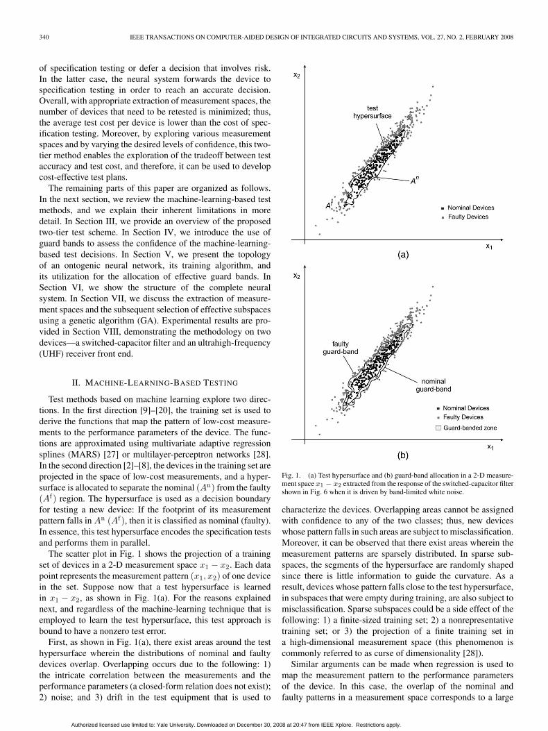
The scatter plot in Fig. 1 shows the projection of a trainingset of devices in a 2-D measurement space x1 − x2. Each datapoint represents the measurement pattern (x1, x2) of one devicein the set. Suppose now that a test hypersurface is learnedin x1 − x2, as shown in Fig. 1(a). For the reasons explainednext, and regardless of the machine-learning technique that isemployed to learn the test hypersurface, this test approach isbound to have a nonzero test error.

First, as shown in Fig. 1(a), there exist areas around the testhypersurface wherein the distributions of nominal and faultydevices overlap. Overlapping occurs due to the following: 1)the intricate correlation between the measurements and theperformance parameters (a closed-form relation does not exist);2) noise; and 3) drift in the test equipment that is used to

Fig. 1. (a) Test hypersurface and (b) guard-band allocation in a 2-D measure-ment space x1 − x2 extracted from the response of the switched-capacitor filtershown in Fig. 6 when it is driven by band-limited white noise.

characterize the devices. Overlapping areas cannot be assignedwith confidence to any of the two classes; thus, new deviceswhose pattern falls in such areas are subject to misclassification.Moreover, it can be observed that there exist areas wherein themeasurement patterns are sparsely distributed. In sparse sub-spaces, the segments of the hypersurface are randomly shapedsince there is little information to guide the curvature. As aresult, devices whose pattern falls close to the test hypersurface,in subspaces that were empty during training, are also subject tomisclassification. Sparse subspaces could be a side effect of thefollowing: 1) a finite-sized training set; 2) a nonrepresentativetraining set; or 3) the projection of a finite training set ina high-dimensional measurement space (this phenomenon iscommonly referred to as curse of dimensionality [28]).

Similar arguments can be made when regression is used tomap the measurement pattern to the performance parametersof the device. In this case, the overlap of the nominal andfaulty patterns in a measurement space corresponds to a large


STRATIGOPOULOS AND MAKRIS: ERROR MODERATION IN MACHINE-LEARNING-BASED ANALOG/RF TESTING 341

Fig. 2. Flow diagram of the proposed two-tier test scheme.

variance in performance-parameter values for similar measure-ment patterns, and the sparsely distributed subspace problem isequivalent to having few samples available for regression.

In extensive simulations with various devices and mea-surement spaces, the test error (or misclassification) ofhypersurface-based tests has never been reported to be below2% [2]–[8]. In regression-based tests [9]–[20], the error isdefined in terms of the prediction accuracy of the regressionfunctions and the correlation coefficients between the measuredand predicted performance-parameter values. The error of thesubsequent classification step, where the predicted values arecompared to the specification limits promised in the data sheet,is usually omitted. In [20], it is shown by using real data froma high-performance WLAN 802.11a/b/g radio transceiver thatthe test error can be as high as 14% when considering thepredicted value of the chain gain parameter. Regression-basedtest methods have the comparative advantage that they providea prediction of the individual performance parameters, thusallowing diagnosis and multibinning.

However, if go/no-go testing, which is essentially a binaryclassification problem, is the primary objective, then solving anintermediate harder problem (i.e., regression) entails a possibleloss of pertinent information available in the training data.Thus, intuitively, when regression is used as the underlyinglearning method, it is expected that the test error will be of atleast similar magnitude to the error of a test hypersurface. Acomparative study to examine the test error when using variousmachine-learning methods is outside the scope of this paper.

In short, to date, it has not been possible to identify a low-cost measurement pattern for any analog/RF device, which,when processed by even the most powerful learning machines,results in an acceptable test-error rate for industrial standards.Thus, additional effort is necessary in order to capitalize on thelow cost of machine-learning-based testing and to make thisapproach competitive, in terms of test accuracy, to specificationtesting.

III. OVERVIEW OF TWO-TIER TEST SCHEME

In this paper, we propose to locate the ambivalent areas inthe measurement space in order to identify the devices for

which the machine-learning-based test decisions are prone toerror. In particular, we propose to allocate guard bands suchthat the measurement space is partitioned into three regions:two regions of predominantly nominal and faulty devices,respectively, and a zone interjected in between that containsa mixed distribution. Fig. 1(b) shows a possible allocation ofguard bands in the measurement space x1 − x2, with the gray-shaded area representing the guard-banded zone. The nominal(faulty) guard band has the entire nominal (faulty) populationon one side, i.e., it guards the nominal (faulty) population.

The guard bands facilitate a two-tier test scheme, as shownin Fig. 2. All fabricated devices go through the first tier, wherethe low-cost pattern of measurements is obtained. The positionof the guard bands in the corresponding measurement spaceis encoded in the neural system through a training routine,which is executed prior to the testing phase and only oncefor any production run. During the testing phase, the neuralsystem examines the relative location of the footprint of themeasurement pattern with respect to the guard-banded zone.If it falls outside the guard-banded zone, then the device isassigned to the respective class, i.e., the neural system infers theresults of specification testing from the measurement pattern,with low test error εr. Otherwise, if it falls in the guard-bandedzone, the device is deemed suspect to misclassification, and theneural system suggests that further action be taken. In this case,the device is directed to the second tier, where it is retestedthrough the standard specification testing in order to reach anaccurate decision.

By enlarging the area of the guard-banded zone, the test errorεr of the first tier is reduced at the expense of retesting moredevices. In the two limits, the guard-banded zone contains theentire device distribution, or the guard bands merge onto thetest hypersurface of Fig. 1(a). Thus, if ε′r denotes the error ofthe test hypersurface and Nr denotes the percentage of devicesthat go through the second tier, then εr drops from ε′r to zeroas Nr increases. In practice, in a discriminative measurementspace, the guard bands can be allocated such that εr approacheszero when a small fraction Nr of devices are retested.

Now, let Ci and Ti denote the test cost per second and thetest time of the ith tier, respectively. Let also Cs and Ts denotethe test cost per second and the test time, respectively, when



the standard specification testing is applied to every fabricateddevice. The average test cost per device for the proposedapproach can be modeled as

C = C1 · T1 + C2(Nr) · T2(Nr). (1)

By using a first-order Taylor approximation, C2(Nr) can bewritten as

C2(Nr) = C2(Nr = 1) +dC2(Nr)

dNr

∣∣∣∣Nr=1

· (Nr − 1)

= Cs + Ch +dC2(Nr)

dNr

∣∣∣∣Nr=1

· (Nr − 1)

= Cs + Ch + C∗(Nr) (2)

where Ch is the test cost per second overhead from handlersthat are used to transfer the devices to the tester in the secondtier, and

C∗(Nr) =dC2(Nr)

dNr

∣∣∣∣Nr=1

· (Nr − 1) ≤ 0. (3)

The test time of the second tier can be expressed as

T2(Nr) = Nr · Ts

= Nr · (T es + Th) (4)

where T es is the electrical specification test time, and Th is the

handling time spent to transfer the devices to the tester in thesecond tier. Equation (1) now becomes

C = C1 · T1 + Nr · (Cs + Ch + C∗(Nr)) · (T es + Th) . (5)

Note that Ch = Th = 0 if the devices do not need to be trans-ferred to another tester to undergo specification testing.

Therefore, if the inequality

C1 · T1 + Nr · (Ch + C∗(Nr)) · (T es + Th)

1 − Nr · T es +ThTs

< Cs · Ts (6)

holds, then

C < Cs · Ts (7)

which means that the test cost is reduced while maintaining theaccuracy of the specification testing.

As previously hinted, given a measurement space, εr and Nr

can be traded off by varying the area of the guard-banded zone.Thereby, and through the exploration of various measurementspaces, a tradeoff curve between εr and C is drawn. This curveallows test engineers to devise cost-effective test plans thattarget different test-quality objectives.

IV. GUARD-BAND ALLOCATION

Guard banding has been mentioned in [11] as also an optionfor the regression-based methods. Therein, guard bands aredefined as a percentile deviation from the device-specificationlimits, but no experimental data is reported regarding the re-sulting percentage of retested devices. In addition, within the

Fig. 3. Steps in the guard-band allocation.

context of specification-test compaction [29], guard bands areallocated by perturbing the entire test hypersurface by a prede-fined distance, thus creating a guard-banded zone of constantwidth. This rigidity of the guard-band allocation method mightinadvertently enclose areas with nonoverlapping populations,resulting in an unnecessarily large percentage of the retesteddevices. Instead, in the proposed method, the guard bandsare viewed as independent decision boundaries and, thus, areallocated regardless of the position of the test hypersurface.

Each guard band is allocated separately to perfectly classifyall the training patterns of the guarded class and, under thisconstraint, to provide an optimum classification for the trainingpatterns of the opposite class. Without loss of generality, con-sider the allocation of the nominal guard band, which is shownon the left-hand side of Fig. 3. First, we draw hyperspheres ofradius Dn centered at nominal training patterns, as shown inFig. 3(a). The radius Dn is defined as

Dn =1

Nn

∑q∈Cn

minp∈Cf

‖�xq − �xp‖ (8)

where �xk is the measurement pattern of training instance k, Cn

and Cf denote the nominal and faulty classes, respectively, ‖ · ‖is the Euclidian norm, and Nn is the number of nominal patterns



in the training set. Faulty training patterns p are successivelypaired with all nominal training patterns q, and if they liewithin distance Dn from the nominal training patterns, i.e., ifthe inequality

‖ �xq − �xp ‖< Dn (9)

holds, then they are temporarily excluded from the trainingset, as shown in Fig. 3(b). After the faulty training patternshave been cleared out of the overlapping areas, the ontogenicneural network described in detail in Section V is employed toallocate the nominal guard band, which is shown in Fig. 3(b).The dual procedure, shown in Fig. 3(c) and (d), is followed toallocate the faulty guard band using a distance Df , which isdefined similarly to Dn in (8). The guard-banded zone is thearea enclosed between the two guard bands, which is gray-shaded in Fig. 3(e).

V. ONTOGENIC NEURAL NETWORK

The guard bands are, in essence, decision boundaries fortesting new devices. In Section V-A, we refer to previous workon this topic, pointing out the limitations that motivate ourchoice of the ontogenic neural network. Next, in Section V-B,we present the topology of the ontogenic neural network.In Section V-C, we discuss its training algorithm, and inSection V-D, we show a heuristic inductive principle to achieveoptimal generalization.

A. Decision Boundaries for Testing Devices

In the past, decision boundaries have been allocated us-ing Fisher’s linear discriminants [2], logistic discriminationanalysis [4], linear-perceptron networks [3], [5], feedforwardneural networks with sigmoidal hidden units [6], [7], andpolynomial kernel transformations [8].

In [2]–[5], the problem is decomposed into M two-classseparation problems that are solved individually, where M isthe number of single-ended device specifications. In particular,as shown in Fig. 4(a), for each single-ended specification µ,a hyperplane bµ is allocated in the measurement space suchthat the maximum possible separation between the nominal andfaulty instances in the training set (with respect to specificationµ) is obtained. In essence, each hyperplane bµ creates two re-gions An(µ) and Af(µ): Instances that fall into An(µ) (Af(µ))are classified as nominal (faulty) with respect to specificationµ. Note that this approach assumes single convex decisionregions, which, as discussed in [8], is not always the case. Theoverall acceptance region An is then approximated by the union⋃M

µ=1 An(µ), which is bounded by the hyperplane segments.However, the decision boundaries are, in general, nonlinear[for example, in Fig. 4(a), the optimal decision boundary is anellipsoid], and thus, a crude approximation with hyperplanesresults in an error. Furthermore, there is an additional errorfactor resulting from individually optimizing the location ofeach of the M decision boundaries. In particular, each decisionboundary is allocated such that it minimizes misclassificationthroughout the entire distribution of measurement patterns.

Fig. 4. Projection of instances of a state variable filter with six single-endedspecifications (M = 6) on a 2-D measurement space x3 − x4. (a) Piecewiselinear approximation of the decision boundary. (b) Individual allocation ofdecision boundaries induces error.

Thus, it also tries to minimize misclassification in areas thatare distant from the acceptance region, which is interpreted asmapping the measurement patterns into the proper faulty class.This, however, is unnecessary, and in addition, it affects thepositioning of the segments of the hyperplanes around whichthe unique nominal class is separated from the 2M − 1 faultyclasses. To view this, consider Fig. 4(b), where Fig. 4(a) isredrawn showing the boundary of the acceptance region andthe measurement patterns distributed across boundaries b5 andb6 only. It can be seen that there exist boundaries b′5 and b′6which would yield a better classification with regard to allspecifications. Yet, b5 and b6 are chosen in place of b′5 and b′6because, with respect to individual specifications, they providea better classification throughout the measurement space.

In [8], polynomial hypersurfaces are allocated in the mea-surement space instead of hyperplanes, but the error resulting



from the individual allocation is still not addressed. In [6]and [7], a feedforward neural network is used that can po-tentially draw decision boundaries of arbitrary order withoutthe need to decompose the problem. However, the networktopology (i.e., the number of hidden units) that generalizeswell on new device instances is not known a priori and canonly be identified empirically by a trial-and-error procedure thatrequires significant computational effort.

As opposed to [6] and [7], the ontogenic neural networkthat we chose to use is constructed successively, in a way thatenables it to adaptively acquire the necessary connectivity thatproduces a decision boundary of appropriate order.

B. Topology

The neural network is trained using data from a set ofdevice instances, which is denoted by St. The performanceparameters of each device k ∈ St are measured explicitly inorder to associate it with a status bit tk, where tk = +1 if kis nominal, i.e., k ∈ Cn, and tk = −1 if k is faulty, i.e., k ∈ Cf .Each instance k ∈ St is also associated with a d-dimensionalmeasurement pattern �xk ∈ Rd. The training set (�x1, t1),(�x2, t2), . . . , (�x|St|, t|St|) is used to optimize the adaptive pa-rameters of the neural network. The classification error on thetraining set is defined as

ESt =1

|St|∑k∈St

hEC(�xk

)(10)

where hEC is the error counting function: hEC(�xk) = 1 if thepattern �xk is misclassified, and hEC(�xk) = 0 otherwise.

As explained in Section V-A, since the order of the decisionboundary is not known a priori, assuming a fixed networktopology limits the range of feasible boundaries. Instead, theproposed neural network learns the boundary constructively,starting with the input layer and dynamically adding layers(ontogenicity) until it matches the intrinsic complexity of theproblem at hand. A comprehensive discussion on constructivealgorithms for neural networks can be found in [30].

In particular, the proposed neural network is constructedusing the 1-pyramid algorithm [31] that successively placeslayers of single neurons above the existing ones. The firstneuron y1 receives inputs from the d measurements. Each suc-cessive neuron yi receives inputs from the d measurements andfrom each neuron below itself. In order for the algorithm to han-dle the real-valued measurements, each neuron above the firstlayer also receives an extra attribute that is the projection of thed-dimensional measurement vector onto a parabolic surface

xd+1 =d∑

i=1

x2i . (11)

Each newly added neuron takes over the role of the outputneuron, and the network growth continues until a satisfactorysolution for the learning problem is found. The complete archi-tecture of the network is shown in Fig. 5.

The neuron model used herein is an �-input threshold logicunit, also known as perceptron [28], that computes the thresh-

Fig. 5. Topology of the ontogenic neural network.

old function of the weighted sum of its inputs �vi ∈ R� :yi(�vi) = −1 for �wT

i �vi < 0 and yi(�vi) = +1 for �wTi �vi ≥ 0.

�wTi = [wi0 , wi1 , . . . , wi�

] is the adaptive weight vector, andthe weight wi0 is referred to as the bias. Here, �v1 = �x, �wT

1 =[w10 , w11 , . . . , w1d

] and �vi = (�x, xd+1, yi−1, . . . , y1), �wTi =

[wi0 , . . . , wid+1 , wi,yi−1 , . . . , wi,y1 ] for i > 1. Since �vi is afunction of �x, in the following, we use yi(�xk) = yi(�vk

i (�xk))to denote the output of the neural network at layer i whenthe measurement pattern �xk is applied at its inputs. Now, letyi(�xk) = +1 and yi(�xk) = −1 refer to pass and fail decisions,respectively, for instance k. Then, we want to select weightssuch that �wT

i �vki < 0 for all �xk ∈ Cf and �wT

i �vki ≥ 0 for all

�xk ∈ Cn.The perceptron has a simple geometrical representation. It

divides linearly its input space by a hyperplane, which iscomposed by the set of solutions to equation �wT

i �vi = 0, suchthat its output yi is +1 on one side of the hyperplane and−1 on the other side. Because of the extra attribute xd+1 in(11) and the input from the preceding neurons, this hyperplanetranslates into a nonlinear hypersurface, denoted by fi, whenit is projected in the original d-dimensional space of measure-ments. Therefore, nonlinear decision boundaries are formed bytraining a sequence of linear perceptrons. This property is veryuseful since, as we discuss in Section VII, it allows the use ofthis network for a fast evaluation of measurement spaces andselection of subspaces in an optimization framework.Theorem 1: Let f be the optimal decision boundary at which

ESt = 0. The aforementioned constructive algorithm produces



a sequence of decision boundaries {fi} that, in the limit,converges to f , i.e., limi→∞ ‖f − fi‖ = 0.

Proof: For each pattern �xp, define

εp =12· min

q =p

d∑i=1

(xpi − xq

i )2

k = maxp,q

d∑i=1

(xpi − xq

i )2

> εp.

Suppose that pattern �xp is misclassified at layer (i − 1), i.e.,yi−1(�xp) = −tp. Then, if we select the following weights

wi0 = tp

k + εp −

d∑j=1

(xp

j

)2

wij= 2tpxp

j , j = 1, . . . , d

wid+1 = − tp

wi,yi−1 = k

wi,yj= 0, j = i − 2, i − 3, . . . , 1

the net input of the ith neuron is

�wTi �vp

i = wi0 +d+1∑j=1

wijxp

j +i−1∑j=1

wi,yjyj(�xp)

= tp

k + εp −

d∑j=1

(xp

j

)2

+

d∑j=1

2tp(xp

j

)2

− tpd∑

j=1

(xp

j

)2 + kyi−1(�xp)

= tpεp.

Since εp > 0, the pattern �xp is correctly classified by the newlayer i. Consider now any pattern �xq = �xp that is correctlyclassified at layer (i − 1), i.e., yi−1(�xq) = tq. Then

�wTi �vq

i =wi0 +d+1∑j=1

wijxq

j +i−1∑j=1

wi,yjyj(�xq)

= tp

k + εp −

d∑j=1

(xp

j

)2

+

d∑j=1

2tpxpjx

qj

− tpd∑

j=1

(xq

j

)2 + kyi−1(�xq)

= tp (k + εp − ε′) + ktq

= tq(

tp

tqk′ + k

)

where ε′ =∑d

i=1(xpi − xq

i )2 > εp, and k′ = k + εp − ε′.

Since 0 < k′ < k, the pattern �xp continues to be classifiedcorrectly after the addition of layer i. Therefore, there exist

weights that will reduce ESt whenever a new layer is addedto the network. Since the number of training patterns isfinite, eventual convergence to ESt = 0 is guaranteed. Inthe following section, we discuss a training algorithm thatgenerates such weights. �

C. Training a Layer

The distributions of nominal and faulty training measurementpatterns are separable at layer i if the following condition holds:

(�wT

i �vki

)tk > 0 ∀k. (12)

In order to reduce ESt at layer i, (12) suggests that we selecta weight vector �wi that minimizes the following error function,which is known as perceptron criterion:

Eperc(�wi) = −∑

k∈St:yi(�xk) =tk

(�wT

i �vki

)tk. (13)

Here, the summation is over all patterns in the training set,which are misclassified by the current weight vector �wi. Theerror function is the sum of a number of positive terms and isequal to zero if all patterns are correctly classified. The searchin the space of weights is performed by applying the thermalperceptron learning rule [32]

w(τ+1)ij

= w(τ)ij

+α

2�vk

j

(tk − yi(�xk)

)e

−|�wTi

�vki |

T (14)

where α > 0. This corresponds to a simple learning procedure:We cycle through all patterns in the training set and test eachpattern, in turn, using the current set of weight values. If thepattern �xk is correctly classified, then we proceed to the next;otherwise, we add α�vk

j e−|�wTi �vk

i |/T to the current weight vector

if �xk ∈ Cn, or we subtract α�vkj e−|�wT

i �vki |/T if �xk ∈ Cf . This

procedure successively reduces the error in (13) [28].The exponential tail in (14) controls the correction of weights

based on the location of the misclassified pattern �xk withrespect to the decision boundary. |�wT

i �vki | is a measure of this

distance. In turn, the temperature T controls how stronglythe changes are attenuated for large values of |�wT

i �vki |. As an

intuition, one can imagine a zone surrounding the decisionboundary. The boundary moves only if an erroneously classifiedpattern falls within this zone. The temperature is annealed froman initial value To to zero, causing a gradual reduction ofthe extent of the sensitive zone. In the limit of T → 0, thezone disappears altogether, and the perceptron is stable, i.e., itstraining has been completed. Best results are obtained when αis reduced at the same time as T is (see [32] for the rationalesupporting this approach).

The thermal learning rule outperforms other knownperceptron-based learning algorithms [33], provided that thetemperature is chosen appropriately. In particular, T shouldbe of the same order of magnitude as the range of values of�wT

i �vki . We followed the suggestion in [34]. T decreases from

To (initially 1) to zero during 500 cycles through the trainingset. Since �wT

i �vki might vary considerably for different device



instances, we calculate the average value of |�wTi �vk

i | over theset of device instances 〈|�wT

i �vki |〉k over each cycle. At the end

of each cycle, To is set to To = (2To + 2〈|�wTi �vk

i |〉k)/3. Thetemperature T is then set to γTo, where γ (initially 1) decreaseslinearly with each cycle to reach zero after 500 cycles. α is setto 0.1γ.

D. Training the Network

The network-training procedure corresponds to an iterativereduction of ESt . However, as training progresses and newlayers are added, there comes a point where the network startsto overfit the training data. This can be observed by examiningthe classification error on an independent set of devices, whichat first keeps decreasing and then starts increasing. The abilityof the network to correctly classify previously unseen deviceinstances, other than those included in St, is called generaliza-tion. In order to find the effective complexity of the network,such that it achieves the best possible generalization, we followan early stopping inductive principle. More specifically, duringtraining, the generalization at each layer is monitored on a sec-ond independent set of device instances (holdout set) denotedby Sh, and after training is complete, the network is pruneddown to the layer that scores the best generalization. At thislayer, an unbiased estimate of the generalization is computedon a third independent set of devices (test set) denoted by Ste.Since, in our case, the decision boundary is used as a guardband, the generalization is measured on the device instancesbelonging to the class that is being guarded. For the nominalguard band, the generalization error is estimated as

P̂ nSte

=1

|Ste|∑

k∈Stek∈Cn

hEC(�xk)

=1

|Ste|∑

k∈Stek∈Cn

(1 − yeff(�xk)

2

)(15)

where yeff denotes the output of the layer that has scored thebest generalization on Sh during training. The set of devicesin Ste, whose measurement pattern falls in the nominal region,can be expressed as

Snte =

{k ∈ Ste : yeff

(�xk

)= 1

}. (16)

By analogy, the generalization error for the faulty guard band isgiven by

P̂ fSte

=1

|Ste|∑

k∈Stek∈Cf

hEC(�xk)

=1

|Ste|∑

k∈Stek∈Cf

(1 + yeff(�xk)

2

)(17)

and the set of devices in Ste, whose measurement pattern fallsin the faulty region, is

Sfte =

{k ∈ Ste : yeff(�xk) = −1

}. (18)

VI. NEURAL SYSTEM

The neural system in Fig. 2 comprises a committee of twoontogenic neural networks that allocate the nominal and faultyguard bands. It requires O(L2 + L · d) computations to exam-ine the relative position of a measurement pattern with respectto the guard bands, where L is the number of perceptrons inthe ontogenic neural networks, and d is the dimensionality ofthe input measurement pattern. The process time of the neuralsystem is a very small fraction of the total test time T1 ofthe first tier. Estimates of Nr and εr are computed on Ste. Inparticular, Nr is equal to the percentage of devices in Ste whosemeasurement pattern falls in the guard-banded zone

Nr =

∣∣Sfte

⋂Sn

te

∣∣|Ste|

(19)

and εr is equal to the sum of the generalization errors of the twoguard bands

εr = P̂ fSte

+ P̂ nSte

. (20)

Evidently, given a measurement space, the aforementionedtradeoff between εr and Nr can be explored by using distancesλfDf and λnDn to clear the overlapping areas and by varyingλf and λn around one. As we increase λf or λn, Nr increases,and εr decreases. In particular, for every measurement space,there exist λf and λn such that εr = 0. More tradeoff pointscan be collected by repeating this procedure for various mea-surement spaces. Note that the neural system is unbiased, i.e.,εr > 0 corresponds to both test escapes and yield loss. If test-escape elimination is of higher importance, a larger λf can beused such that the faulty guard band is pushed deeper into thenominal region. In this case, the tradeoff is obtained by onlyvarying λn.

VII. MEASUREMENT-SPACE EXTRACTION

The effectiveness of the two-tier test scheme is measured bythree parameters, namely, the test cost of the first tier (C1 · T1),the test error of the first tier (εr), and the percentage of devicesthat go through the second tier (Nr). These three parameters,in turn, depend on the choice of the measurement pattern.

In order to guarantee a low test time T1, the measure-ment pattern should be low dimensional and should be ex-tracted by switching the device to a minimum number of testconfigurations, preferably only one. In order to guarantee alow test cost per second C1, the measurement pattern shouldbe extracted using a low-cost assortment of test equipment.To satisfy this objective for multigigahertz RF devices, it isnecessary to avoid the use of expensive RF testers and tointerface the methodology to the existing mixed-signal testequipment [35]. For example, in [10] and [19], the authorsapply the concept of modulation and demodulation to translatea baseband test stimulus to the RF spectrum and to convert theresponse back to a baseband signature. In [12], it is proposed toundersample the RF response using a noise reference and, then,to obtain the Fourier harmonics in the spectrum. In [13] and[16], the authors embed sensors (e.g., peak and rms detectors,



differential-topology sensors, and recursive sensors) into theRF signal paths to extract dc or low-frequency signals. Thedc and low-frequency signals can also be extracted by addingdesign-for-testability structures on-chip (e.g., loopback paths,offset cancellation digital-to-analog converters implementedat each low-frequency block output, and additional internalprobes) [20]. A test configuration for time-division multiple-access RF power amplifiers is proposed in [17], where thetransient-current response to a slow ascending ramp signal iscaptured. A test configuration for RF transceivers is proposed in[18], where the transmitted signal is looped back to the receiver.The measurement space is extracted from the spectrum at theoutput of the receive mixer. In [36], it is proposed to observe thequiescent current signature when the power supply is ramped indiscrete steps.

Achieving low Nr requires that the measurement space pro-vides adequate discrimination between the nominal and faultydistributions such that the ambivalent areas constitute only asmall fraction of it. In contrast, εr depends only on the para-meters λf and λn and the dimensionality of the measurementspace. In particular, we only need to circumvent the curse ofdimensionality by keeping the ratio of |St| to the dimensionalityof the measurement space high.

Given a test configuration, we initially extract dI measure-ments, where dI is large in order to increase the probability ofextracting useful measurements. Then, we search in the space ofcandidate measurements to select a subspace of dimensionalityd < dI that best meets our objective on the tradeoff curveεr − Nr. In particular, we can pursue the minimization ofNr under the constraint εr ≤ δ, δ ∈ [0, ε′r), where εr = ε′r forNr = 0. Note that since the training set has a finite size, εrand Nr can take discrete values k/|St|, where k ∈ N, k ≤ |St|.The points on the optimal tradeoff curve are largely known asPareto-optimal solutions.

Recent comparative studies [37] show that GAs are the mostsuitable for large-scale measurement selection problems [38].GAs start with a base population of chromosomes and generatesuccessive populations through an intrinsically parallel searchprocess that mimics the mechanics of natural selection andgenetics [39]. In the search for subsets of measurements, asubset is encoded in a chromosome as a d-element bit string,with the ith bit denoting the presence or the absence of theith measurement. GAs evolve by the juxtaposition of schemata(bit templates), resulting in rapid optimization of the targetfitness function. Instead of running a GA many times by usinga fitness function that emphasizes one particular Pareto-optimalsolution for each time, we use a multiobjective GA, called theNSGA-II [40], in order to find multiple Pareto-optimal so-lutions in one single simulation run. The NSGA-II uses bi-nary tournament selection, crossover, and mutation operatorsto generate offspring populations. It also includes elitism anda parameterless diversity-preservation mechanism to ensure agood spread of the Pareto-optimal solutions.

VIII. EXPERIMENTAL RESULTS

The proposed method is evaluated on a fifth-order ellipticswitched-capacitor filter, which is shown in Fig. 6, using syn-

Fig. 6. Ladder realization of the fifth-order elliptic switched-capacitor filter[41].

thetic data from simulation analysis and an off-the-shelf RFdevice using real data. The studied RF device is a monolithicintegrated UHF receiver front end that contains a low-noiseamplifier (LNA) and a balanced mixer. The course of eachexperiment is as follows.

1) We start with a representative set of N device instances.Each instance k, k = 1, . . . , N , undergoes full specifi-cation testing in order to associate it with an accuratenominal or faulty label tk.

2) We select a test configuration, a test stimulus, and aninitial set of dI measurements.

3) We obtain the dI measurements on all instances of N .4) The dI measurements are normalized in order to avert

skewing of the distance between two measurement pat-terns in the computation of Df and Dn. Moreover, inpractice, normalization speeds up the training phase ofthe neural system. The normalized measurements aregathered in dI-dimensional vectors �xk, k = 1, . . . , N .

5) The N device instances are divided into training, holdout,and test sets.

6) The NSGA-II algorithm is run to identify the Pareto-optimal subspaces of the dI-dimensional measurementspace. The parent population of measurement subspaces



Fig. 7. Test configuration for the switched-capacitor filter of Fig. 6.

at each generation is 200, and the algorithm terminatesafter 100 generations. The crossover and mutation proba-bilities are set to 0.9 and 1/dI, respectively. Each mea-surement subspace is evaluated by training the neuralsystem in order to estimate εr and Nr. The parametersλf and λn are set to one.

7) After the NSGA-II converges, for every Pareto-optimalmeasurement subspace, we retrain the neural system us-ing different values of λf and λn. We examine all combi-nations as λf and λn vary from 0.25 to 1.5 at a 0.25 step.Thus, for every Pareto-optimal measurement subspace,we obtain an additional set of 36 points (εr and Nr),which may improve the Pareto-optimal front.

8) We plot the tradeoff curve εr − Nr that connects thepoints of the Pareto-optimal front.

The costs Ch and C∗(Nr) in (5) depend on a large numberof factors and may vary widely across the industry. In order toprovide estimates of the average test cost per device, we adopta simplified model

C = C1 · T1 + Nr · Cs · (T es + Th) (21)

which can be deduced from the general model of (5) by settingCh = C∗(Nr) = 0. Note that the aforementioned simplifiedmodel is not necessarily optimistic since C∗(Nr) ≤ 0, and thus,Ch + C∗(Nr) could attain a negative value for low Nr. Onthe contrary, the simplified model is pessimistic if the devicesdo not need to be transferred to another tester to undergospecification testing, in which case Ch = 0.

Next, we describe each of the experiments in detail.

A. Switched-Capacitor Filter

We generated N = 2000 instances of the switched-capacitorfilter by Monte Carlo analysis, letting various designparameters follow a normal distribution, centered at their nom-inal values with a 3% standard deviation. The design para-meters considered include the switched-capacitor values andthe geometry, oxide thickness, threshold voltage, body-effectcoefficient, and junction capacitances of the transistors in theop-amps. Catastrophic shorts and opens in the MOS switchesare excluded since they generate outlier points in the faultydistribution and, thus, do not affect the positioning of the guardbands. N/2 instances are assigned to the training set, whereasN/4 instances are assigned to each of the holdout and test sets.The performance parameters considered include the ripples in

Fig. 8. Power spectrum of the unfiltered LFSR bit sequence output [42].

the passband and stopband, gain errors, group delay, phaseresponse, and total harmonic distortion.

As a test stimulus, we use white noise limited up to afrequency multiple of the bandwidth of the switched-capacitorfilter [24]. Intuitively, this is a promising stimulus since itcontains infinite tones that can generate persistently excitingresponse waveforms. The band-limited white noise can bedigitally synthesized by passing the pseudorandom bit sequenceoutput of a linear feedback shift register (LFSR) through alow-pass filter (LPF) [42]. The filtered bit pattern is appliedto the switched-capacitor filter through a driving buffer. ThedI measurements are obtained by digitizing its response at dI

equidistant points. The complete test configuration is shownin Fig. 7.

The parameters of the test configuration, namely, the clockfrequency of the LFSR fclk, the length of the LFSR m, and thecutoff frequency of the LPF, can be defined by examining thepower spectrum of the unfiltered LFSR output, which is shownin Fig. 8. It can be seen that the envelope of the spectrum isproportional to the square of (sin x)/x. The spectrum is flatwithin ±0.1 dB up to 12% of fclk and drops rapidly beyondits −3-dB point of 0.44fclk. Thus, low-pass filtering with ahigh-frequency cutoff of 5%–10% of fclk will convert theLFSR output to a band-limited white-noise voltage. Since asharp cutoff characteristic is not required, simple RC filter-ing suffices. According to the aforementioned discussion, fclk

must be chosen such that 0.1fclk ≥ ν · BW, where BW is the



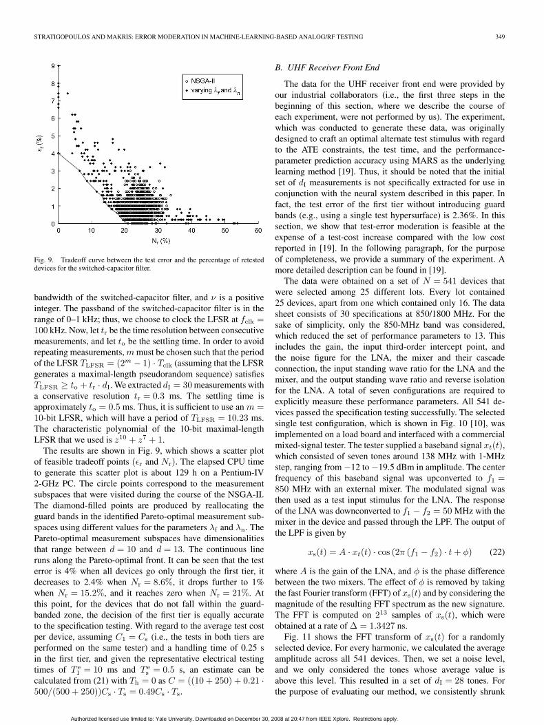
Fig. 9. Tradeoff curve between the test error and the percentage of retesteddevices for the switched-capacitor filter.

bandwidth of the switched-capacitor filter, and ν is a positiveinteger. The passband of the switched-capacitor filter is in therange of 0–1 kHz; thus, we choose to clock the LFSR at fclk =100 kHz. Now, let tr be the time resolution between consecutivemeasurements, and let to be the settling time. In order to avoidrepeating measurements, m must be chosen such that the periodof the LFSR TLFSR = (2m − 1) · Tclk (assuming that the LFSRgenerates a maximal-length pseudorandom sequence) satisfiesTLFSR ≥ to + tr · dI. We extracted dI = 30 measurements witha conservative resolution tr = 0.3 ms. The settling time isapproximately to = 0.5 ms. Thus, it is sufficient to use an m =10-bit LFSR, which will have a period of TLFSR = 10.23 ms.The characteristic polynomial of the 10-bit maximal-lengthLFSR that we used is z10 + z7 + 1.

The results are shown in Fig. 9, which shows a scatter plotof feasible tradeoff points (εr and Nr). The elapsed CPU timeto generate this scatter plot is about 129 h on a Pentium-IV2-GHz PC. The circle points correspond to the measurementsubspaces that were visited during the course of the NSGA-II.The diamond-filled points are produced by reallocating theguard bands in the identified Pareto-optimal measurement sub-spaces using different values for the parameters λf and λn. ThePareto-optimal measurement subspaces have dimensionalitiesthat range between d = 10 and d = 13. The continuous lineruns along the Pareto-optimal front. It can be seen that the testerror is 4% when all devices go only through the first tier, itdecreases to 2.4% when Nr = 8.6%, it drops further to 1%when Nr = 15.2%, and it reaches zero when Nr = 21%. Atthis point, for the devices that do not fall within the guard-banded zone, the decision of the first tier is equally accurateto the specification testing. With regard to the average test costper device, assuming C1 = Cs (i.e., the tests in both tiers areperformed on the same tester) and a handling time of 0.25 sin the first tier, and given the representative electrical testingtimes of T e

1 = 10 ms and T es = 0.5 s, an estimate can be

calculated from (21) with Th = 0 as C = ((10 + 250) + 0.21 ·500/(500 + 250))Cs · Ts = 0.49Cs · Ts.

B. UHF Receiver Front End

The data for the UHF receiver front end were provided byour industrial collaborators (i.e., the first three steps in thebeginning of this section, where we describe the course ofeach experiment, were not performed by us). The experiment,which was conducted to generate these data, was originallydesigned to craft an optimal alternate test stimulus with regardto the ATE constraints, the test time, and the performance-parameter prediction accuracy using MARS as the underlyinglearning method [19]. Thus, it should be noted that the initialset of dI measurements is not specifically extracted for use inconjunction with the neural system described in this paper. Infact, the test error of the first tier without introducing guardbands (e.g., using a single test hypersurface) is 2.36%. In thissection, we show that test-error moderation is feasible at theexpense of a test-cost increase compared with the low costreported in [19]. In the following paragraph, for the purposeof completeness, we provide a summary of the experiment. Amore detailed description can be found in [19].

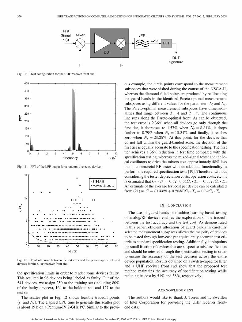
The data were obtained on a set of N = 541 devices thatwere selected among 25 different lots. Every lot contained25 devices, apart from one which contained only 16. The datasheet consists of 30 specifications at 850/1800 MHz. For thesake of simplicity, only the 850-MHz band was considered,which reduced the set of performance parameters to 13. Thisincludes the gain, the input third-order intercept point, andthe noise figure for the LNA, the mixer and their cascadeconnection, the input standing wave ratio for the LNA and themixer, and the output standing wave ratio and reverse isolationfor the LNA. A total of seven configurations are required toexplicitly measure these performance parameters. All 541 de-vices passed the specification testing successfully. The selectedsingle test configuration, which is shown in Fig. 10 [10], wasimplemented on a load board and interfaced with a commercialmixed-signal tester. The tester supplied a baseband signal xt(t),which consisted of seven tones around 138 MHz with 1-MHzstep, ranging from −12 to −19.5 dBm in amplitude. The centerfrequency of this baseband signal was upconverted to f1 =850 MHz with an external mixer. The modulated signal wasthen used as a test input stimulus for the LNA. The responseof the LNA was downconverted to f1 − f2 = 50 MHz with themixer in the device and passed through the LPF. The output ofthe LPF is given by

xs(t) = A · xt(t) · cos (2π (f1 − f2) · t + φ) (22)

where A is the gain of the LNA, and φ is the phase differencebetween the two mixers. The effect of φ is removed by takingthe fast Fourier transform (FFT) of xs(t) and by considering themagnitude of the resulting FFT spectrum as the new signature.The FFT is computed on 213 samples of xs(t), which wereobtained at a rate of ∆ = 1.3427 ns.

Fig. 11 shows the FFT transform of xs(t) for a randomlyselected device. For every harmonic, we calculated the averageamplitude across all 541 devices. Then, we set a noise level,and we only considered the tones whose average value isabove this level. This resulted in a set of dI = 28 tones. Forthe purpose of evaluating our method, we consistently shrunk



Fig. 10. Test configuration for the UHF receiver front end.

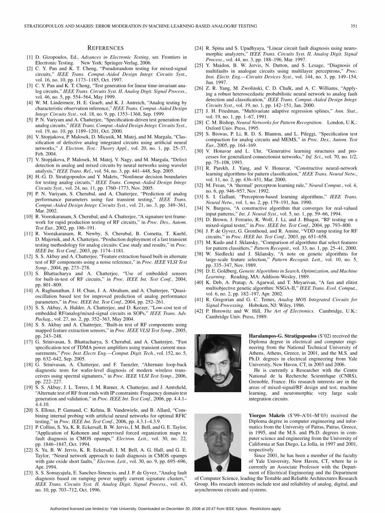
Fig. 11. FFT of the LPF output for a randomly selected device.

Fig. 12. Tradeoff curve between the test error and the percentage of retesteddevices for the UHF receiver front end.

the specification limits in order to render some devices faulty.This resulted in 96 devices being labeled as faulty. Out of the541 devices, we assign 250 to the training set (including 80%of the faulty devices), 164 to the holdout set, and 127 to thetest set.

The scatter plot in Fig. 12 shows feasible tradeoff points(εr and Nr). The elapsed CPU time to generate this scatter plotis about 19 h on a Pentium-IV 2-GHz PC. Similar to the previ-

ous example, the circle points correspond to the measurementsubspaces that were visited during the course of the NSGA-II,whereas the diamond-filled points are produced by reallocatingthe guard bands in the identified Pareto-optimal measurementsubspaces using different values for the parameters λf and λn.The Pareto-optimal measurement subspaces have dimension-alities that range between d = 4 and d = 7. The continuousline runs along the Pareto-optimal front. As can be observed,the test error is 2.36% when all devices go only through thefirst tier, it decreases to 1.57% when Nr = 5.51%, it dropsfurther to 0.79% when Nr = 10.24%, and finally, it reacheszero when Nr = 28.35%. At this point, for the devices thatdo not fall within the guard-banded zone, the decision of thefirst tier is equally accurate to the specification testing. The firsttier achieves a 36% reduction in test time compared with thespecification testing, whereas the mixed-signal tester and the lo-cal oscillators to drive the mixers cost approximately 48% lessthan a commercial RF tester with an adequate functionality toperform the required specification tests [19]. Therefore, withoutconsidering the tester depreciation costs, operation costs, etc., itis estimated that C1 · T1 = 0.52 · 0.64Cs · Ts = 0.3328Cs · Ts.An estimate of the average test cost per device can be calculatedfrom (21) as C = (0.3328 + 0.2835)Cs · Ts = 0.62Cs · Ts.

IX. CONCLUSION

The use of guard bands in machine-learning-based testingof analog/RF devices enables the exploration of the tradeoffbetween the test accuracy and the test cost. As demonstratedin this paper, efficient allocation of guard bands in carefullyselected measurement subspaces allows the majority of devicesto be tested through low-cost yet equivalently accurate test cri-teria to standard specification testing. Additionally, it pinpointsthe small fraction of devices that are suspect to misclassificationand should be retested through the specification testing in orderto ensure the accuracy of the test decision across the entiredevice population. Results obtained on a switch-capacitor filterand a UHF receiver front end show that the proposed testmethod maintains the accuracy of specification testing whilereducing its cost by 51% and 38%, respectively.

ACKNOWLEDGMENT

The authors would like to thank J. Torres and T. Swettlenof Intel Corporation for providing the UHF receiver front-end data.



REFERENCES

[1] D. Gizopoulos, Ed., Advances in Electronic Testing, ser. Frontiers inElectronic Testing. New York: Springer-Verlag, 2006.

[2] C. Y. Pan and K. T. Cheng, “Pseudorandom testing for mixed-signalcircuits,” IEEE Trans. Comput.-Aided Design Integr. Circuits Syst.,vol. 16, no. 10, pp. 1173–1185, Oct. 1997.

[3] C. Y. Pan and K. T. Cheng, “Test generation for linear time-invariant ana-log circuits,” IEEE Trans. Circuits Syst. II, Analog Digit. Signal Process.,vol. 46, no. 5, pp. 554–564, May 1999.

[4] W. M. Lindermeir, H. E. Graeb, and K. J. Antreich, “Analog testing bycharacteristic observation inference,” IEEE Trans. Comput.-Aided DesignIntegr. Circuits Syst., vol. 18, no. 9, pp. 1353–1368, Sep. 1999.

[5] P. N. Variyam and A. Chatterjee, “Specification-driven test generation foranalog circuits,” IEEE Trans. Comput.-Aided Design Integr. Circuits Syst.,vol. 19, no. 10, pp. 1189–1201, Oct. 2000.

[6] V. Stopjakova, P. Malosek, D. Micusik, M. Matej, and M. Margala, “Clas-sification of defective analog integrated circuits using artificial neuralnetworks,” J. Electron. Test.: Theory Appl., vol. 20, no. 1, pp. 25–37,Feb. 2004.

[7] V. Stopjakova, P. Malosek, M. Matej, V. Nagy, and M. Margala, “Defectdetection in analog and mixed circuits by neural networks using waveletanalysis,” IEEE Trans. Rel., vol. 54, no. 3, pp. 441–448, Sep. 2005.

[8] H.-G. D. Stratigopoulos and Y. Makris, “Nonlinear decision boundariesfor testing analog circuits,” IEEE Trans. Comput.-Aided Design Integr.Circuits Syst., vol. 24, no. 11, pp. 1760–1773, Nov. 2005.

[9] P. N. Variyam, S. Cherubal, and A. Chatterjee, “Prediction of analogperformance parameters using fast transient testing,” IEEE Trans.Comput.-Aided Design Integr. Circuits Syst., vol. 21, no. 3, pp. 349–361,Mar. 2002.

[10] R. Voorakaranam, S. Cherubal, and A. Chatterjee, “A signature test frame-work for rapid production testing of RF circuits,” in Proc. Des., Autom.Test Eur., 2002, pp. 186–191.

[11] R. Voorakaranam, R. Newby, S. Cherubal, B. Cometta, T. Kuehl,D. Majernik, and A. Chatterjee, “Production deployment of a fast transienttesting methodology for analog circuits: Case study and results,” in Proc.IEEE Int. Test Conf., 2003, pp. 1174–1181.

[12] S. S. Akbay and A. Chatterjee, “Feature extraction based built-in alternatetest of RF components using a noise reference,” in Proc. IEEE VLSI TestSymp., 2004, pp. 273–278.

[13] S. Bhattacharya and A. Chatterjee, “Use of embedded sensorsfor built-in-test of RF circuits,” in Proc. IEEE Int. Test Conf., 2004,pp. 801–809.

[14] A. Raghunathan, J. H. Chun, J. A. Abraham, and A. Chatterjee, “Quasi-oscillation based test for improved prediction of analog performanceparameters,” in Proc. IEEE Int. Test Conf., 2004, pp. 252–261.

[15] S. S. Akbay, A. Halder, A. Chatterjee, and D. Keezer, “Low-cost test ofembedded RF/analog/mixed-signal circuits in SOPs,” IEEE Trans. Adv.Packag., vol. 27, no. 2, pp. 352–363, May 2004.

[16] S. S. Akbay and A. Chatterjee, “Built-in test of RF components usingmapped feature extraction sensors,” in Proc. IEEE VLSI Test Symp., 2005,pp. 243–248.

[17] G. Srinivasan, S. Bhattacharya, S. Cherubal, and A. Chatterjee, “Fastspecification test of TDMA power amplifiers using transient current mea-surements,” Proc. Inst. Electr. Eng.—Comput. Digit. Tech., vol. 152, no. 5,pp. 632–642, Sep. 2005.

[18] G. Srinivasan, A. Chatterjee, and F. Taenzler, “Alternate loop-backdiagnostic tests for wafer-level diagnosis of modern wireless trans-ceivers using spectral signatures,” in Proc. IEEE VLSI Test Symp., 2006,pp. 222–227.

[19] S. S. Akbay, J. L. Torres, J. M. Rumer, A. Chatterjee, and J. Amtsfield,“Alternate test of RF front ends with IP constraints: Frequency domain testgeneration and validation,” in Proc. IEEE Int. Test Conf., 2006, pp. 4.4.1–4.4.10.

[20] S. Ellouz, P. Gamand, C. Kelma, B. Vandewiele, and B. Allard, “Com-bining internal probing with artificial neural networks for optimal RFICtesting,” in Proc. IEEE Int. Test Conf., 2006, pp. 4.3.1–4.3.9.

[21] P. Collins, S. Yu, K. R. Eckersall, B. W. Jervis, I. M. Bell, and G. E. Taylor,“Application of Kohonen and supervised forced organization maps tofault diagnosis in CMOS opamps,” Electron. Lett., vol. 30, no. 22,pp. 1846–1847, Oct. 1994.

[22] S. Yu, B. W. Jervis, K. R. Eckersall, I. M. Bell, A. G. Hall, and G. E.Taylor, “Neural network approach to fault diagnosis in CMOS opampswith gate oxide short faults,” Electron. Lett., vol. 30, no. 9, pp. 695–696,Apr. 1994.

[23] S. S. Somayajula, E. Sanchez-Sinencio, and J. P. de Gyvez, “Analog faultdiagnosis based on ramping power supply current signature clusters,”IEEE Trans. Circuits Syst. II, Analog Digit. Signal Process., vol. 43,no. 10, pp. 703–712, Oct. 1996.

[24] R. Spina and S. Upadhyaya, “Linear circuit fault diagnosis using neuro-morphic analyzers,” IEEE Trans. Circuits Syst. II, Analog Digit. SignalProcess., vol. 44, no. 3, pp. 188–196, Mar. 1997.

[25] Y. Maidon, B. W. Jervis, N. Dutton, and S. Lesage, “Diagnosis ofmultifaults in analogue circuits using multilayer perceptrons,” Proc.Inst. Electr. Eng.—Circuits Devices Syst., vol. 144, no. 3, pp. 149–154,Jun. 1997.

[26] Z. R. Yang, M. Zwolinski, C. D. Chalk, and A. C. Williams, “Apply-ing a robust heteroscedastic probabilistic neural network to analog faultdetection and classification,” IEEE Trans. Comput.-Aided Design Integr.Circuits Syst., vol. 19, no. 1, pp. 142–151, Jan. 2000.

[27] J. H. Friedman, “Multivariate adaptive regression splines,” Ann. Stat.,vol. 19, no. 1, pp. 1–67, 1991.

[28] C. M. Bishop, Neural Networks for Pattern Recognition. London, U.K.:Oxford Univ. Press, 1995.

[29] S. Biswas, P. Li, R. D. S. Blanton, and L. Pileggi, “Specification testcompaction for analog circuits and MEMS,” in Proc. Des., Autom. TestEur., 2005, pp. 164–169.

[30] V. Honavar and L. Uhr, “Generative learning structures and pro-cesses for generalized connectionist networks,” Inf. Sci., vol. 70, no. 1/2,pp. 75–108, 1993.

[31] R. Parekh, J. Yang, and V. Honavar, “Constructive neural-networklearning algorithms for pattern classification,” IEEE Trans. Neural Netw.,vol. 11, no. 2, pp. 436–451, Mar. 2000.

[32] M. Frean, “A ‘thermal’ perceptron learning rule,” Neural Comput., vol. 4,no. 6, pp. 946–957, Nov. 1992.

[33] S. I. Gallant, “Perceptron-based learning algorithms,” IEEE Trans.Neural Netw., vol. 1, no. 2, pp. 179–191, Jun. 1990.

[34] N. Burgess, “A constructive algorithm that converges for real-valuedinput patterns,” Int. J. Neural Syst., vol. 5, no. 1, pp. 59–66, 1994.

[35] D. Brown, J. Ferrario, R. Wolf, J. Li, and J. Bhagat, “RF testing on amixed-signal tester,” in Proc. IEEE Int. Test Conf., 2004, pp. 793–800.

[36] J. P. de Gyvez, G. Gronthoud, and R. Amine, “VDD ramp testing for RFcircuits,” in Proc. IEEE Int. Test Conf., 2003, pp. 651–658.

[37] M. Kudo and J. Sklansky, “Comparison of algorithms that select featuresfor pattern classifiers,” Pattern Recognit., vol. 33, no. 1, pp. 25–41, 2000.

[38] W. Siedlecki and J. Sklansky, “A note on genetic algorithms forlarge-scale feature selection,” Pattern Recognit. Lett., vol. 10, no. 5,pp. 335–347, Nov. 1989.

[39] D. E. Goldberg, Genetic Algorithms in Search, Optimization, andMachineLearning. Reading, MA: Addison-Wesley, 1989.

[40] K. Deb, A. Pratap, A. Agarwal, and T. Meyarivan, “A fast and elitistmultiobjective genetic algorithm: NSGA-II,” IEEE Trans. Evol. Comput.,vol. 6, no. 2, pp. 182–197, Apr. 2002.

[41] R. Gregorian and G. C. Temes, Analog MOS Integrated Circuits forSignal Processing. Hoboken, NJ: Wiley, 1986.

[42] P. Horowitz and W. Hill, The Art of Electronics. Cambridge, U.K.:Cambridge Univ. Press, 1989.

Haralampos-G. Stratigopoulos (S’02) received theDiploma degree in electrical and computer engi-neering from the National Technical University ofAthens, Athens, Greece, in 2001, and the M.S. andPh.D. degrees in electrical engineering from YaleUniversity, New Haven, CT, in 2003 and 2006.

He is currently a Researcher with the CentreNational de la Recherche Scientifique (CNRS),Grenoble, France. His research interests are in theareas of mixed-signal/RF design and test, machinelearning, and neuromorphic very large scaleintegration circuits.

Yiorgos Makris (S’99–A’01–M’03) received theDiploma degree in computer engineering and infor-matics from the University of Patras, Patras, Greece,in 1995, and the M.S. and Ph.D. degrees in com-puter science and engineering from the University ofCalifornia at San Diego, La Jolla, in 1997 and 2001,respectively.

Since 2001, he has been a member of the facultyof Yale University, New Haven, CT, where he iscurrently an Associate Professor with the Depart-ment of Electrical Engineering and the Department

of Computer Science, leading the Testable and Reliable Architectures ResearchGroup. His research interests include test and reliability of analog, digital, andasynchronous circuits and systems.


ieee transactions on computer-aided …gxm112130/papers/tcad08.pdfdigital object identiﬁer...

Documents