ieee transactions on dependable and secure …tdsc07.pdf · the first approaches to group...

Online Diagnosis and Recovery: On the Choiceand Impact of Tuning Parameters

Marco Serafini, Student Member, IEEE, Andrea Bondavalli, Member, IEEE, and

Neeraj Suri, Senior Member, IEEE

Abstract—A sequenced process of Fault Detection followed by the erroneous node’s Isolation and system Reconfiguration (node

exclusion or recovery), that is, the FDIR process, characterizes the sustained operations of a fault-tolerant system. For distributed

systems utilizing message passing, a number of diagnostic (and associated FDIR) approaches, including our prior algorithms, exist in

literature and practice. Invariably, the focus is on proving the completeness and correctness (all and only the faulty nodes are isolated)

for the chosen fault model, without explicitly segregating permanent from transient faulty nodes. To capture diagnostic issues related to

the persistence of errors (transient, intermittent, and permanent), we advocate the integration of count-and-threshold mechanisms into

the FDIR framework. Targeting pragmatic system issues, we develop an adaptive online FDIR framework that handles a continuum of

fault models and diagnostic protocols and comprehensively characterizes the role of various probabilistic parameters that, due to the

count-and-threshold approach, influence the correctness and completeness of diagnosis and system reliability such as the fault

detection frequency. The FDIR framework has been implemented on two prototypes for automotive and aerospace applications. The

tuning of the protocol parameters at design time allows a significant improvement with respect to prior design choices.

Index Terms—Error detection, transient faults, online diagnosis, system reliability, recovery.

Ç

1 INTRODUCTION

A fault-tolerant system is designed to provide sustaineddelivery of services despite encountered perturbations.

The ability to accurately detect, diagnose, and recover fromfaults1 in an online manner (that is, during systemoperation) constitutes an important aspect of fault tolerance.This Fault Detection followed by Isolation and systemReconfiguration (FDIR) process has two primary objectives:to consistently identify a faulty node so as to restrict its effecton system operations and to support the process of systemrecovery via isolation and reconfiguration of the systemresources to sustain ongoing system operations. If FDIR isperformed as an online procedure [32], [33], then thisprovides an effective capability of resource management,responding promptly to the appearance and disappearanceof faults, with a small duration of system susceptibility tosubsequent fault accumulation.

However, the capacity of consistently identifying faultynodes does not necessarily imply the ability to select thebest recovery action. For example, an overpessimistic FDIRcan overreact and exclude all nodes encountering transient

faults, thus reducing available resources and impactingreliability. A possible solution is the use of count-and-threshold approaches [6], which established a fundamentalbasis for online recording and handling of transients. Itenables accumulating “Fault Detection” information oversystem operations before triggering the most appropriate“Isolation and Reconfiguration” actions. The health of anode is thus determined, based on the persistency andrecurrence of its failures, by postponing its isolation, even ifsome errors are observed.

In this paper, we introduce a generic FDIR frameworkfor integrating existing distributed diagnosis approacheswith a count-and-threshold algorithm. As the relativeoccurrences and ratios of permanent, intermittent, andtransient hardware faults are matters of ongoing debate,especially as technology changes continually affect theserates [9], we develop a modeling methodology to probabil-istically study the effects of such rate variations and toguide the choice of design parameters accordingly.

Our focus is on distributed systems, but the analysis andderived metrics are general enough to be adapted for thetuning of any periodic error detection subsystem, similar to[6], [7]. Despite appearing intuitive, most of the obtainedresults have not, to our knowledge, been comprehensivelydeveloped, linking both the diagnostic protocol and thecount-and-threshold aspects.

The process of local detection, global diagnosis, isolation,and recovery from a given fault instance is a multifacetedproblem. The specific aspects addressed in this paper arelisted as follows:

. The capability of the FDIR processes to accuratelycapture the “severity” of the error. For example,errors of core-system-level functions are more severethan those of optional application-level functions

IEEE TRANSACTIONS ON DEPENDABLE AND SECURE COMPUTING, VOL. 4, NO. 4, OCTOBER-DECEMBER 2007 1

. M. Serafini and N. Suri are with the Department of Computer Science, TUDarmstadt, Hochschulstr. 35, 64289 Darmstadt, Germany.E-mail: {marco, suri}@informatik.tu-darmstadt.de.

. A. Bondavalli is with the Dipartimento di Sistemi ed Informatica,Universita degli Studi di Firenze, Viale Morgagni, 65, 50134 Firenze,Italy. E-mail: [email protected].

Manuscript received 22 May 2006; revised 2 Apr. 2007; accepted 5 June 2007;published online 19 June 2007.For information on obtaining reprints of this article, please send e-mail to:[email protected], and reference IEEECS Log Number TDSC-0062-0506.Digital Object Identifier no. 10.1109/TDSC.2007.70210.

1. In reality, one detects the manifestation of a fault, that is, an “error.”Thus, error detection is the accurate term to use [19]. Nevertheless, weutilize the more conventionally accepted term of “fault detection” for theFDIR terminology.

1545-5971/07/$25.00 � 2007 IEEE Published by the IEEE Computer Society

and, consequently, will result in faster isolation andreconfiguration. It should be emphasized that theprocess of fault detection itself may not necessarilyprovide information on the severity of an error,unless specific error detection mechanisms exist,which correspond to established severity types.

. The capability to capture the “duration” of an error(the time period when it is continuously observed)and its “recurrence” (the frequency of successiveobservations). The desired response of the FDIRoperations to a transient, regardless of its severitylevel, can be very different from the response to apermanent fault. For example, should we isolate anode encountering only transients?

. The impact of different settings of the parameters ofthe count-and-threshold algorithm on the resilienceand the reliability of the system. For example, iferror detection is executed too frequently, then thesame fault will be detected multiple times, increas-ing the likelihood of isolating nodes, regardless ofthe transient nature of the fault. This can unnecessa-rily degrade system redundancy.

These issues motivate our research on FDIR processes.We highlight the trade-offs in the tuning of the designparameters, discuss the trends, and propose methods to aidtuning of the diagnostic process as tailored to specificsystem characteristics and requirements. We show how theapproach is applicable to prototype systems for automotiveand aerospace applications. The probability of isolation dueto transient faults could almost be ruled out in bothscenarios by considering that all functions, includingsafety-critical ones, show a certain degree of tolerance totransient outages. However, nodes with dormant faultsactivating as seldom as every 10 hours on the average canbe isolated by appropriately tuning our FDIR algorithm.

1.1 Related Work

A variety of approaches exist, which address the FDIRprocess (or parts of it), and a complete survey is beyond thescope of this paper. We limit ourselves to a brief overviewof the main existing work in the field.

The theoretical problem of diagnosis was set up in thePreparata-Metze-Chien (PMC) model [26]. The focus of thiswork and of many related approaches was on characteriz-ing system configurations, fault sets, and assignments,where n active components (units) are able to diagnose, inthe presence of up to t faulty units, all the faulty units (one-step t-diagnosability) or at least one of them (sequentialt-diagnosability). The problem of assignment has beenfurther developed from many viewpoints, trying to definesufficient and necessary conditions when only somecombinations of the elements are known. Many extensionsexist to the PMC assumptions, considering the fact that afault might not always manifest in a permanent manner [5],[23] or extending the analysis from multiprocessor systemsto distributed systems [17], [30]. An excellent survey on thestrong similarities between diagnosis and consensus pro-blems in distributed systems can be found in [2].

An important element for the timeliness of onlinediagnosis, especially in real-time systems requiring timely

reaction to faults, is the ability to execute diagnostic testswithout interrupting system operation, that is, withoutexplicit testing capabilities. A well-known solution is thecomparison approach [4], [24], [28], where multiple nodesexecute the same task, and the outcomes are compared byother nodes.

If nodes are assumed to be fail silent, then groupmembership protocols can be used for FDIR operations.They ensure that all nodes have a consistent view of thecurrent set of correct nodes. The first definition of the groupmembership problem and a solution in asynchronoussystems were developed within the ISIS project [3]. One ofthe first approaches to group membership for synchronoussystems was proposed in [10]. The time-triggered protocol(TTP) [16] intertwines a membership protocol with clocksynchronization in synchronous systems.

Our previous work [33] introduced a family of distrib-uted diagnostic algorithms for synchronous systems basedon the Customizable Fault/Error Model (CFEM) [32], wherethe fault assumptions can be adapted to meet the faulthypothesis of the core fault-tolerant protocols of the system(for example, clock synchronization). One advantage is thatdiagnosis is not considered as an offline and fault-freeprocedure but as an online core fault-tolerant mechanismfully integrated in the system fault-tolerant strategy. Insteadof executing dedicated performance-impacting tests like inthe PMC model or constraining the allocation of applica-tion-level tasks to nodes like in the comparison approach, ituses error detection information derived by the execution offundamental system-level activities like message deliveryand clock synchronization to diagnose the system. Thisapproach is complementary to graph-based application-level approaches. The diagnostic protocol is seen as aspecial case of consensus under the CFEM. The need forrecording the duration and recurrence of errors and toassign them different severity levels has been pointed out.

Most previous diagnostic services provide snapshot-level information about a single manifestation of a fault.After a fault is detected, nodes are declared as either alwayspermanent or always transient faulty. An evaluation of theeffect on system reliability of these two different policieswas conducted in [20]. The intuitive result was that optimalreliability is not attained by either.

In practice, nodes oscillate between faulty and correctbehavior. To handle this, a range of mechanisms collectivelycalled “count-and-threshold” schemes were established inour previous work [6], [7]. The idea is that “componentsshould be kept in the system until the benefit of keeping thefaulty component online is offset by the greater probabilityof multiple (hence, catastrophic) faults.” Apart from the classof permanent faults, when the component always fails everytime it is activated, a basic discrimination is done in thecontext of temporary errors spanning intermittents andtransients: the first are due to faults internal to thecomponent and show a high occurrence rate, whicheventually might turn them to permanent faults, whereasthe second are due to reasons that are external to thecomponent, generally have an uncorrelated occurrence rate,and should not determine the exclusion of the component.Therefore, after detecting a transient, it is advocated to wait

2 IEEE TRANSACTIONS ON DEPENDABLE AND SECURE COMPUTING, VOL. 4, NO. 4, OCTOBER-DECEMBER 2007

and see if the error reappears before isolating the compo-nent. Error counters for each component are incrementedwhen the node fails and decremented when it delivers acorrect service. When a chosen threshold value is exceeded,the corresponding component is isolated.

The fundamental advantages, disadvantages, and trade-offs involved in using online count-and-threshold mechan-isms and in defining the related thresholds have beencharacterized in [6], where a generic class of low-overheadcount-and-threshold mechanisms, called �-count, is de-fined. This model was elegantly extended in [7] to includedouble-threshold mechanisms, where a component istemporarily excluded after the first threshold is exceededbut still given an opportunity to be reintegrated and wheremore complex error distributions are considered. Theapplicability of the analysis is restricted to the case whereerror duration does not exceed the diagnostic period. Also,the presence of an “error detection subsystem” is assumed,which, for distributed diagnosis, means the existence of anunderlying error detection, aggregation, and agreementservice to support the threshold counting. The powerful�-count model has also been implemented in the GenericUpgradable Architecture for Real-time Dependable Systems(GUARDS) architecture [25] for distributed diagnosis. Abinary accusation on the node health is shared usingconsensus, voted upon, and given as input to the �-function.

Many proposed diagnostic approaches use similarcustom parametric schemes, paired with sophisticatedstatistical techniques, to discriminate between transientand intermittent faults [15], [21]. However, due to theircomplexity, these are not usable in an online mode.

1.2 Our Contributions

Most cited works on distributed diagnosis have focused onestablishing the correctness and completeness of thediagnostic approaches for varied fault models. An oftenused assumption is that once a node fails, it must beisolated as fast as possible. This implicitly rules out thepragmatic issue that healthy nodes can suffer from transientoutages that can be detected and treated but still do notrequire isolation. We introduce and examine a genericonline FDIR framework, which is able to generalize thepreviously proposed distributed diagnosis protocols and toenhance them with count-and-threshold techniques inorder to effectively handle transient faults.

In particular, our aim is to 1) determine the effect of theduration and recurrence of faults on the effectiveness of theonline diagnosis protocols and 2) ascertain the sensitivityand the trade-offs of choices of some selected FDIR designparameters2 in determining the correctness and complete-ness of the FDIR protocols and in improving systemreliability.

We consider system parameters that can influence theeffectiveness of the FDIR process. For example, in asynchronous distributed system, every node exchangesdata at an epoch, also known as the communication round. Aserror detection takes place over each round, we can also

consider it the minimal achievable diagnostic round. Overeach communication round, the system health is “sampled”by the different nodes and exchanged by using thediagnostic protocol. In this context, the assumption thaterrors manifest only over a single round, as characterized inprevious analyses, is not adequate. The length of thediagnostic round is a parameter that, together with othercount-and-threshold parameters, will influence the like-lihood with which a node is excluded from systemoperation. In fact, if the round is too short, then a transientfault may be perceived as permanent and, consequently,lead to pessimistic resource isolation. This can be particu-larly problematic for long-duration missions. On the otherhand, if the round length is too large, then one wouldexpect large diagnostic latencies in the system. Thisincreases the probability of coincident errors within thesame round and might be undesirable for critical applica-tions with short mission times and requirements of rapidresponse to perturbations.

A discrimination between transient and intermittent orpermanent faults solves two key problems: the depletion ofsystem resources (and, consequently, of system resilience tofaults) caused by the isolation of transient faulty nodes andthe reduced coverage of the system fault hypothesis (that is,the assumption on the number of faults tolerated by thecore system protocols within a given time window) ifintermittent faulty nodes are left operative. Our contribu-tion is to study the choice of diagnostic round length andother system parameters within an architectural context tohighlight the correctness, completeness, and reliabilitytrade-offs. We consider the following design parameters:

. Diagnostic round rate. The rate at which nodesexchange diagnostic data, aggregate it and, conse-quently, update penalties and rewards.

. Penalty counter threshold values. The number oftemporally correlated diagnostic rounds, after whichan erroneous node gets isolated.

. Reward counter threshold values. The number ofdiagnostic rounds, after which a node (previouslysuspected as erroneous) displaying correct behaviorgets readmitted into the system as a “good” node.

. Penalty increments. The penalties assigned aftererrors with varied severities are detected.

We provide a generic FDIR framework that can beinstantiated in multiple different implementations. Along-side, we provide stochastic techniques to examine the maintrends related to the identified parameters. Furthermore, wereport on the use of the FDIR approach and the relatedtuning techniques in prototypes for the automotive andaerospace domains. We discuss how different severitylevels can be established and describe how, by means of afiner tuning, better settings could be found at design time,that is, without carrying out measurements on an imple-mented system.

The paper is organized as follows: Section 2 details thegeneric online fault diagnosis process supporting the FDIRalgorithm, which is discussed in Section 3. Section 4introduces the diagnostic measures and models used toevaluate the goodness of the design choices related to theFDIR process. Section 5 details the main trends involved in

SERAFINI ET AL.: ONLINE DIAGNOSIS AND RECOVERY: ON THE CHOICE AND IMPACT OF TUNING PARAMETERS 3

2. We concentrate our analysis on parameters representing phenomenathat are considered here for the first time, whereas we skip others alreadystudied in [7], since their role is well established.

tuning the parameters. Section 6 reports on the practicalapplication of the FDIR approach to prototypes from theautomotive and aerospace domains. Section 7 summarizesour results and insights.

2 A GENERIC FDIR FRAMEWORK

A generic FDIR framework consists of four key steps:

1. collection of local syndromes from internal andinternode local error detection,

2. dissemination of the local syndromes,3. analysis to consistently diagnose the faulty nodes,

and4. (possibly) isolation of the faulty nodes and

reconfiguration.

The first three steps are generally carried out by adistributed diagnostic protocol. We propose to separatethe diagnosis of faults (1-3) from the decision on theisolation of the node 4) and to isolate a node only if multipleinstances of the diagnostic protocol indicate a sustainedfaulty behavior. In the following, we describe each of thesesteps in detail.

In order to establish a basis for our analysis, we present asystem model and an associated count-and-thresholdapproach to support online diagnosis and FDIR. Weconsider a distributed system framework by using around-based (synchronous) message dispersal protocol.Essentially, such a communication model implies thatmessages are broadcast and received by the system nodesperiodically at specific times following an a priori determi-nistic schedule. A nonfaulty receiver node can identify thesender of an incoming message and can detect the absenceor time deviance (early or late) for an expected message. It isimportant to mention that we have chosen a synchronoussystem model for simplicity of presentation. Our analysisdeveloped in this paper can directly be extended to partiallysynchronous models (for example, timed asynchronous [11]or asynchronous augmented with failure detectors [8]), aslong as there are mechanisms for 1) periodic error detectionto form local syndromes and 2) authenticated channels toensure that the sender of a message can be correctlyidentified.

As a comprehensive example of how the four steps applyto a distributed diagnostic protocol, we utilize the diag-nostic protocol defined in [29] as a basic reference. Weconsider a CFEM [32], where faults can be either benign, thatis, each node can locally detect the related errors, ormalicious. The malicious faulty nodes can either senderroneous information symmetrically or asymmetrically.The latter case is the classical Byzantine case. The ability of anode to send correct messages in the designated timewindows is used as a periodic diagnostic test. Noassumption is made on the persistence of faults, as thecorrect delivery of each message is diagnosed indepen-dently. The protocol is able to diagnose bursts of multipleconcurrent benign faults and to tolerate malicious faults.

2.1 Error Detection, Dissemination, and Analysis

During error detection, each node collects the evidence onsystem health that are locally observed at runtime. Besides

self-checks executed by each node to detect internal errorsand ensure error containment, online internode errordetection is achieved through the constant monitoring ofthe message exchange. The result of this online monitoringoccurring during system operation is condensed by eachnode into a local syndrome representing its local view of thecorrectness of the other nodes.

The granularity of the information stored in the localsyndrome can vary. Different error classes, for example,missing message, late message, early message, wrongsyntax, and corrupted cyclical redundancy checking(CRC), can be defined and associated with different severitylevels. Also, errors impacting different system services withdifferent criticality levels can be reported separately,allowing different fault-handling actions.

Due to malicious and symmetric faults, this localdetection information is not sufficient to identify and locatefaults. Therefore, local syndromes are disseminated toachieve a global view. This is periodically done at discretepoints in time at the boundaries of what we call diagnosticrounds. Generally, the communication rounds and thediagnostic rounds coincide as local error detection anddissemination take place during each message exchangeround.

After dissemination, each node analyzes the receivedinformation based on the fault model of the diagnosticprotocol and derives a global and consistent snapshot view ofthe system state. The snapshot view assesses whether (andhow) a node is faulty and ensures the following propertiesunder the given fault assumption:

. Correctness. A correct node is never diagnosed faulty.

. Completeness. All benign nodes are diagnosed faulty.

. Consistency. All nodes agree on the same set of faultynodes at each diagnostic round.

All of the local syndromes are collected to build asyndrome matrix, where each row represents a localsyndrome, and each column contains all the local viewson the health of a certain node. Similar to the second roundof the protocol OMHð1Þ [22], the analysis consists ofperforming a Hybrid Majority voting along the columns.The protocol ensures correctness, completeness, and con-sistency. In particular, it is able to detect all benign faultsand those asymmetric faults that are detected by at least amajority of nodes. The presence of malicious faults cannotalways be detected but does not disrupt consistency. A linkfault is equated to a node fault, but the more sophisticatednode-link discrimination approaches such as [13], [27] canbe used as well. However, transient external faults on thecommunication network can be filtered out by using ourFDIR algorithm.

2.2 Isolation of Unhealthy Nodes

The diagnostic protocol ensures that each node obtains, ateach diagnostic round, consistent information on themanifested faults. This is called a snapshot view, as itrefers to the detection of fault manifestations within a singlediagnostic round.

Current approaches define isolation policies solely basedon this snapshot view. Our purpose is to observe thebehavior of the system over a given time interval before


taking a decision on whether to isolate a node or not.

Relying on correct, complete, and consistent snapshot views

provided to each node by the distributed diagnosis

protocol, we develop an expanded �-function, extending

on [7], that accumulates this data over successive diagnostic

rounds to discriminate between unhealthy and healthy

(although, at times, faulty) nodes.Fault models typically used for diagnostic protocols do

not consider the fact that faults can disappear and reappear,

that is, the duration and recurrence of faults. We extend the

fault models used by the diagnostic protocol and assume

that at a given time, nodes can be

. unhealthy, if they have internal faults and fail in apermanent or intermittent manner, or

. healthy, if they fail only on external transients.

Healthy nodes can become unhealthy during system

operation. We introduce these two terms to distinguish a

node being faulty in a single diagnostic round from a node

showing correlated subsequent failures. The goal of our

FDIR protocol is to isolate only unhealthy nodes, whereas

healthy nodes should be kept operative. In order to make

this discrimination possible, we make two assumptions:

. (A1) Nodes can fail and recover an infinite numberof times.

. (A2) Healthy nodes fail with lower frequency thanunhealthy nodes.

These assumptions do not only arise from intuition but

also reflect experimental results, as in [31].

3 THE PARAMETRIC FDIR ALGORITHM

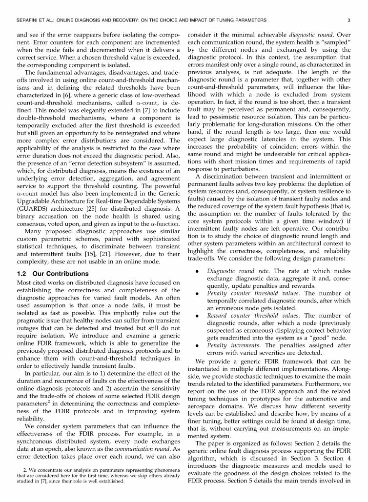
We propose to use a count-and-threshold algorithm on topof the diagnostic protocol to reduce the likelihood ofisolation and increase the availability of healthy nodes incase of external transient faults. Each node executes thealgorithm represented by the flow diagram in Fig. 1a andaccumulates the observations of the health of all nodesobtained through snapshot views by using two values: apenalty counter and a reward counter. We describe theoperations of the algorithm on a single node. As everyupdate of the penalty and reward counters is based on theconsistent snapshot view, it is ensured that all updates areexecuted consistently. Therefore, each node has the samepenalty and reward counters for all nodes in the system. Anode can be in one of the four possible states, eachcorresponding to the four phases of the FDIR algorithm,as depicted in Fig. 1b, namely, Error Free, Health Diagnosis,Isolated, or Recovery.

3.1 Error-Free and Health Diagnosis Phases

In the initial system state, each node is Error Free, and thevalues of the penalty and reward counters (p and r inFig. 1a) are set to 0. The conditional block labeled “Faulty?”represents the content of the consistent snapshot view of thecurrent diagnostic round.

As long as no errors from a node are detected, thealgorithm loops in the Error-Free phase. After the node isdiagnosed faulty for the first time, the system keeps thetarget node under observation for a finite time span toproduce an assessment of its health and to isolate it only ifthe duration or recurrence of errors exceeds a tolerable rate.


Fig. 1. The local online FDIR algorithm for each node. (a) Block diagram. (b) States (phases) that a node can visit. *A “permanency counter” can be

put up to exclude a node as a permanent fault if it continues to remain faulty for a specified number of unsuccessful recovery attempts.

This phase is called Health Diagnosis. Each time a node isdiagnosed faulty, the related penalty counter is increasedby a penalty increment reflecting the severity level. Con-versely, if a node in the Health Diagnosis phase producescorrect messages, then the reward counter is increased by 1but is set to 0 as soon as another error appears. In Fig. 1a,the dashed boxes represent updates of the penalty andreward counters. The Health Diagnosis phase can have twooutcomes (see Fig. 1b): 1) If the penalty counter exceeds apredefined penalty threshold P , then the node is isolated. 2)If the reward counter exceeds a predefined reward thresh-old R, then the diagnostic process is reset by setting bothpenalty and reward counts to 0. This process of updatingand checking p and r is performed at each diagnostic round.

If the diagnostic protocol is capable of discriminatingdifferent severity classes of errors hs1; . . . ; sni, then these canbe ordered in growing degree of criticality. Intuitively, anode showing more severe errors should be assigned higherpenalty increments than other nodes with less severe errorsin order to reach the penalty threshold faster. Therefore,different penalty increments �p ¼ hp1; . . . ; pni can be asso-ciated to different severity levels, where p1 < p2 < . . . < pn.In Section 6, we elaborate on how the choice of variedpenalty increments can be tuned to satisfy desired systemrequirements.

We use two counters and two related thresholds torepresent two different kinds of information. Rewards arerelated to the correlation between subsequent faults. In thealgorithm in Fig. 1a, snapshot views are evaluated aftereach diagnostic round. The reward counter stores thenumber of consecutive fault-free diagnostic rounds that anode under Health Diagnosis displays. If the length of suchrounds is T time units, the reward threshold is thus reachedafter R � T time units without faults. In this case, subsequentfaults are considered uncorrelated with the previous. Onthe other hand, penalties and the penalty threshold P arerelated to the maximum length of tolerated faulty burstsbefore a node is isolated, which is P � T time units.

3.2 Isolated and Recovery Phases

Even though the introduction of the Health Diagnosis phaseincreases the availability of healthy nodes, the likelihoodthat long and bursty transients lead to incorrect nodeisolations cannot generally be ruled out, especially in casesof adverse external conditions or high-severity errors [29].Therefore, we introduce a Recovery phase after nodeisolation, which provides an observation period to handleany residual faults and also to allow reintegrating a nodethat is incorrectly isolated.

If the penalty counter exceeds its threshold, then theHealth Diagnosis phase ends, and the node goes into theIsolated state; that is, it is declared erroneous, and itsparticipation on the ongoing computations in subsequentrounds is restricted. However, even in the Isolated state, theincriminated node continues, as long as it is viable, toparticipate by sending its messages at the prescribedinstants, allowing a selective isolation based on the typeof service that the node provides.

Potentially, the Recovery phase could allow unhealthynodes to be reintegrated. Therefore, reintegrated nodes areassigned a penalty of k > 0 so that successive faultmanifestations will lead to a faster reisolation. The reward

threshold for recovery ðRrÞ does not necessarily need to beequal to the reward threshold for diagnosis ðRÞ and can beadjusted, together with k, to handle this trade-off. Similar tothe Health Diagnosis phase, the Recovery phase alsoreaches an outcome, either bringing the node back to theIsolated state or reintegrating it, after a bounded time of atmost Rr rounds.

In some systems, especially long-life systems, diagnosisis also mandated to signal when a node needs to bereplaced. Representing this case requires that the Recoveryphase in Fig. 1a is executed a finite number of times (forexample, by setting a “permanency counter”), and if thenode is not able to recover, it must be completely excluded.Such behavior is also recommended to limit the additionaloverhead involved in checking the behavior of an unhealthynode. A variation of the algorithm in this sense can be theuse of a double-threshold approach [7], where a faulty nodecan continue accruing penalties after isolation, and if asecond penalty threshold is reached, then the node issignaled for replacement.

4 MODELING THE FDIR EFFECTIVENESS

In the FDIR process, the nodes of a distributed system arereconfigured using penalty and reward counters that areperiodically updated at each diagnostic round until athreshold is reached. Thus, the design issue for onlinediagnosis and FDIR considered in this paper is given asfollows:

Given a system with specific transient and intermittent fault

duration and reappearance times, what are the “best” parameter

settings that minimize wrong isolations and maximize correct

isolations? Note that the notion of “best” can change, depending

on the design goals of the system, that is, whether the objective of

the FDIR approach is to maximize the isolation of unhealthy

nodes, minimize the isolation of healthy nodes, or increase the

overall system reliability.In this section, we define the basis of the model used to

evaluate the effectiveness of the FDIR approach and definestochastic measures for the FDIR effectiveness. Thesemeasures are functions of the specific aspects of the studiedsystem (for example, fault duration and recurrence) and ofthe design parameters (for example, the diagnostic roundrate and the penalty and reward thresholds).

4.1 Measures for FDIR Effectiveness

Of the four phases of the FDIR algorithm, we call the HealthDiagnosis and Recovery phases transitory phases. The reasonis that a node can remain in these phases only for a limitedamount of time, and a diagnostic outcome is ensured withinbounded time. The role of transitory phases is to discrimi-nate between healthy nodes hit only by transient faults andunhealthy nodes showing an intermittently or permanentlyfaulty behavior. The measures for FDIR effectiveness mustreflect the capability of correct discrimination.

For the Health Diagnosis phase, we define two notions ofcompleteness and correctness for healthy and unhealthynodes, which we assign specific names to distinguish themfrom the similarly named properties of the underlyingdiagnostic protocols:


. Accumulated Correctness (or accuracy) is the prob-ability that a healthy node in the Error-Free stateentering the Health Diagnosis phase is not isolated.

. Accumulated Completeness (or coverage) is theprobability that an unhealthy node in the Error-Freestate entering the Health Diagnosis phase is isolated.

As Accumulated Completeness trivially equals 1 forunhealthy nodes displaying permanent faults, we restrictour analysis to intermittent faults.

Besides Accumulated Correctness and Completeness,another measure of interest for the Health Diagnosis phaseis the time needed to isolate unhealthy nodes:

. Diagnostic Latency is the interval between a nodebecoming unhealthy and its isolation.

Even if Health Diagnosis is a transitory phase and isterminated in a bounded time, a node can switch betweenthe Error-Free and Health Diagnosis phases multiple timesbefore being isolated. In [6], [7], the Health Diagnosis phasecan last for an unbounded period of time. Therefore, twodifferent measures were defined to capture this aspect: theoverall diagnostic latency from the first fault appearance inan unhealthy node to its isolation D and the fraction ofunused lifetime of a healthy node NU , that is, the timebetween wrong isolation of a healthy node and its eventualtransition to the unhealthy state divided by the time neededto become unhealthy from the beginning of its operationallife. Our measures can be used to obtain D and NU byconsidering each execution of the Health Diagnosis phase asa Bernoulli trial, where success is node isolation.

Although unhealthy nodes should be kept isolated,healthy nodes should be reintegrated. Similar measurescan be thus defined to describe the behavior of thealgorithm after a node is isolated:

. Stable Correctness is the probability that an isolatedhealthy node entering the Recovery phase is reinte-grated.

. Stable Completeness is the probability that anisolated unhealthy node entering the Recoveryphase is not reintegrated.

The FDIR algorithm is a parametric algorithm. In the restof this section, we relate the measures introduced in thissection to the settings of the parameters.

4.2 Characterization of the System

We consider that nodes can alternate between periods ofcorrect and faulty behavior, as assumed in Section 2.2. After

a fault is activated, errors are observable for a time, whichwe term Time to Recovery (TTR), before they disappear.Eventually, errors will reappear either because of newtransient faults or correlated intermittent faults. The time toerror reappearance is called Time to Failure (TTF). This isdepicted in Fig. 2. We can characterize the behavior of agiven specific system by measuring or estimating theprobabilities of error disappearance and reappearance ineach diagnostic round.

The Health Diagnosis phase begins when a previouslyError-Free node is diagnosed faulty. Nodes can pass fromthe correct to the failed states and back infinitely often(assumption A1). The TTR represents the permanence timein the faulty state before errors disappear and can bemodeled by a continuous stochastic variable X, whoseprobability distribution function (pdf) is fXðtÞ, and whoseCumulative Distribution Function (CDF) is FXðtÞ. Oncerecovered, a node will eventually fail again. The TTFrepresents the permanence time in the correct state and canbe represented by a similar continuous stochastic variableY .

As the count-and-threshold algorithm receives data atdiscrete points in time corresponding to the diagnosticrounds, we study the behavior of the protocol as a discretetime problem, where the time unit is represented by thediagnostic round length T . The pdf of the discrete stochasticvariable bX resulting from X is

fbXðiÞ ¼R iTði�1ÞT fXðtÞdt if i > 0

0 if i ¼ 0:

�ð1Þ

The pdf of the discrete stochastic variable bY can beobtained analogously.

In each diagnostic round following the manifestation

of a fault, there is a probability, called disappearance hazard

dðiÞ, that the fault disappears. It is the discrete hazard

function of fbXðiÞ, that is, the probability of fault

disappearance at diagnostic round i, conditioned by the

fact that the error did not disappear in the previous

round. It can be calculated as

dðiÞ ¼fbXðiÞ

1� FbXði� 1Þ :

Analogously, for correct nodes, we can associate a

reappearance hazard mðiÞ to fbY ðiÞ, that is, a probability of

fault reappearance in each diagnostic round.


Fig. 2. Appearance and disappearance of faults.

We define the stochastic characterization of the specificsystem under study as a quadruple hdhðiÞ;mhðiÞ; duðiÞ;muðiÞicomposed by the disappearance and reappearance hazardsat round i of healthy nodes (dhðiÞ and mhðiÞ) and unhealthynodes (duðiÞ and muðiÞ), respectively.3 Assumption A2 inSection 2.2 can now be formalized by assuming the expectedvalue of the distribution muðiÞ to be much smaller than ofmhðiÞ. The multiple factors that influence dðiÞ and mðiÞ arediscussed in more detail in Section 6.

4.3 Stochastic Models for the FDIR Algorithm

We use the disappearance and reappearance hazards dðiÞand mðiÞ to model subsequent failures of a node over timeinstead of the logical predicates normally used by theexisting diagnostic protocols. The properties of the protocoltherefore become probabilistic and can be obtained bymeans of the stochastic models that we present below. Ascorrect nodes consistently update penalties and rewards, wecan use a single model to study the execution of thetransitory phases of the FDIR algorithm in each correct node.

The measures of Accumulated Correctness and Com-pleteness are defined based on the probability of isolation ofhealthy and unhealthy nodes, respectively, during anexecution of the Health Diagnosis phase. To calculate them,we build a model of how the penalties and rewardsassociated with a node are consistently updated. We modelthe case of unary penalty increments upon errors, but theanalysis can be easily extended to the case of differentincrements associated to varied severity levels. In fact, theprobability of isolation when the penalty increment is 1, andthe penalty threshold is P , is the same as if the increment ispj, and the threshold dP=pje.

Values for dðiÞ and mðiÞ can be either expressed using ananalytical distribution or defined using experimental resultsto assign a probability for each value of i. Regardless, it ispossible to model the behavior of the protocol by using aDiscrete Time Markov Chain (DTMC).

If the disappearance hazard is constant,4 that is, dðiÞ ¼ d,then the probability of isolation of a node after a failure and

a subsequent single execution of the Health Diagnosisphase can be obtained from the simpler DTMC in Fig. 3.Each state is depicted as hp; ri, representing that the nodeunder consideration has accrued consistent penalty counterp and reward counter r. In the initial state h1; 0i, the nodehas just displayed an error. Each transition modelssubsequent diagnostic rounds, where errors may be presentor not. The probabilities of error disappearance andreappearance are d and mðiÞ, respectively. States markedas hp; 0i follow the detection of an error and, consequently, dis only used for their outgoing transitions. The other statesfollow a correct round and have outgoing transitionsdefined in terms of mðiÞ.

In this particular case, the probability of isolation can becalculated (see the Appendix) as5

Pisol ¼ 1� d �YR�1

i¼1

ð1�mðiÞÞ !ðP�1Þ

: ð2Þ

However, if the disappearance hazard is not constant butfollows a generic distribution dðiÞ, then the complexity ofthe model grows, as i must be represented in each state ofthe DTMC.6 We can thus model it by using a higher levelformalism such as the Stochastic Activity Network in Fig. 4and solve it by using a tool like Mobius [12].

The places Faulty and FaultFree in Fig. 4 hold a tokenwhen the node is in the corresponding state. Therefore, inthe initial marking, a token is put in the place Faulty,whereas the place FaultFree is empty. Counters is anextended place that stores the tuple hp; ri rather thansimply tokens. The activity DiagnosticRound represents theexecution of one diagnostic round. It has two casesassociated with the probability of detecting a fault. If thenode is faulty, then the probabilities associated with the twocases are 1� dðiÞ and dðiÞ, respectively, whereas these aremðiÞ and 1�mðiÞ if the node is fault free. The output gatesFaultDetected and NoFaultDetected update the penalty andthe reward counters and check them against the threshold,possibly putting one token into the places Isolated or Reset. Ifthis happens, the activity DiagnosticRound is disabled by theinput gate NotFinished, and the model reaches an absorbingstate. The output gate FaultDetected also adds a token in theplace StripLength, which records the current number ofdiagnostic rounds i from fault occurrence (respectively,disappearance) necessary to determine dðiÞ (and mðiÞ). The


Fig. 3. DTMC for constant dðiÞ ¼ d.

Fig. 4. DTMC for the general case.

3. As notation, we add the subscripts h and u for the measures referringspecifically to unhealthy (intermittent) and healthy (transient) faults. Whenwe refer jointly to both cases, no subscript is added.

4. The fault models of [6], [7], which assume that faults disappears after adiagnostic round, represent a special case, where dðiÞ is constant and equalto d ¼ 1.

5. It can be observed thatQR�1

i¼1 ð1�mðiÞÞ can also be calculated as theprobability that a fault reappears before the reward threshold R is reached;that is, 1� FY ððR� 1Þ � T Þ or, equivalently, 1� FbY ðR� 1Þ (see the Appen-dix for details).

6. For the reappearance hazard mðiÞ, the parameter i is already implicitlydefined by the current reward counter r.

model has two absorbing states characterized by thepresence of a token in Isolate or Reset, respectively. Theprobability that the model reaches the first absorbing stateis Pisol. The number of steps before an absorbing state isreached gives the Diagnostic Latency in terms of diagnosticrounds.

Accumulated Correctness and Completeness can becalculated from Pisol by using the disappearance andreappearance hazards of, respectively, healthy and un-healthy nodes. Accumulated Correctness is the probabilityof not isolating a healthy node, whereas AccumulatedCompleteness is the probability of isolating an unhealthynode.

The Recovery phase can be modeled using a similarDTMC and is simpler, as only reward accumulation needsto be considered. In this case, the probability of reintegra-tion upon error disappearance is the probability that furthererrors do not appear before the Reintegration threshold Rr

is reached:

Preint ¼YRr�1

i¼1

ð1�mðiÞÞ:

As in the previous case, Stable Correctness and Complete-ness can be calculated from this expression by using thereappearance hazard mðiÞ of healthy and unhealthy nodes.Stable Correctness is the probability of reintegrating healthynodes, whereas Stable Completeness is the probability ofnot reintegrating unhealthy nodes.

This model is appropriate in those cases where replace-ment is not considered. There are also cases where a node,after some attempts to recover, is considered permanentlyfaulty and is extracted from the system, as no benefit butonly damage can be envisaged from keeping it operative. Insuch cases, a slight modification of the model is sufficient inorder to count how many times the node enters theRecovery phase before being signaled for replacement.

5 IMPACT OF THE DESIGN PARAMETERS ON

HEALTH DIAGNOSIS

The modeling framework that we have defined previouslyallows system designers to tune the design parametersaccording to the specific system under study. This sectionprovides an insight into the main issues and trendsinvolved with the parameter tuning by evaluating theresulting values of Accumulated Correctness and Comple-teness and Diagnostic Latency (for brevity, these measuresare also respectively termed accuracy, coverage, and latency inthe rest of the paper). An example of harder tuning in adifferent scenario is also described, where the expected TTFfor healthy and unhealthy nodes is similar. Finally, theimpact of the FDIR parameters on reliability is highlighted.

For our trend analysis, we consider a generic auto-motive system. The average TTR E½X� is 5 ms, and weconsider four discrete distributions of bX: binomial, geo-metric (where the hazard dðiÞ is constant), Poisson, anduniform. For finite-support distributions, we assume amaximum TTR Xmax ¼ 10 ms, as in [14]. The smalldifferences in the accuracy and coverage obtained fordifferent distributions of bX confirms that in this case, thesimplified model in Fig. 3 and the related closed-form

analytical expression (2) provide a good approximation.The TTF (transient) for healthy nodes Yh is assumed to beexponentially distributed, with an expected value E½Yh� ¼1; 000 hours, and the TTF (intermittent) for Yu forunhealthy nodes follows a Weibull distribution [31], withincreasing failure rate ð� ¼ 1:4Þ and an expected valueE½Yu� ¼ 1 hour. Therefore, according to assumption A2 inSection 2.2, we assume that E½Yh� > E½Yu�. While conduct-ing sensitivity analysis on each design parameters, we fixthe others to the nominal values P ¼ 5, R ¼ 106, andT ¼ 5 ms. Table 1 summarizes the considered design andsystem parameters with their nominal values. Initially, weconsider unity penalty increments.

5.1 Tuning of the Design Parameters

The analysis confirms that the diagnostic round length has astrong impact on the measures of interest. The longer thediagnostic rounds, the higher the probability of observingan event during a round, either recovery or failure. Theresulting accuracy and coverage are given in Fig. 5a. In thisfigure, as in some other following ones, multiple curvesoverlap with each other. However, all figures displayconformal trends. We can observe the presence of pointsof minimal coverage ðT ¼ 1� 5 msÞ and maximal accuracyðT ¼ 10 ms� 1 secÞ. In fact, if the diagnostic rounds are tooshort, then nodes do not have enough time to recover beforethe penalty threshold is reached and are always isolated. Inthis case, the accuracy is 0, and the coverage is 1. The sameresult is obtained when the diagnostic round is excessivelylong. In this case, the period of correct operation before thecounters are reset becomes too long, and even subsequenttransient faults are considered as correlated. Overall, wecannot consider a setting of the penalty and rewardthresholds as good per se without considering the diagnosticround length.

In Fig. 5a, as well as in the subsequent figures, the resultsobtained using different distributions of the TTR bX aresimilar, especially if both measures are close to 1. Therefore,when a highly refined tuning is not necessary, the geometricdistribution, where dðiÞ ¼ d, can be adopted for theanalysis. This enables using the closed-form analyticalexpression of (2) rather than simulations or numericalanalysis.

The average latency of isolation of unhealthy nodes atvarying values of T is plotted in Fig. 5b. As expected,increasing the length of the diagnostic round also increasesthe time necessary to isolate an unhealthy node. However,for values of T greater than 100 ms, the latency tends togrow much less. The reason is that when the coverage isclose to 1, isolation is usually achieved, in a bounded time,after the first Health Diagnosis following the fault. There-fore, the latency depends on how many error bursts arenecessary to reach the penalty threshold. For finite-supportdistributions, the latency is higher than the one observed forother distribution, especially when diagnostic rounds arelarge enough to make it impossible for a single error burstto determine node isolation. In general, the longer the tail ofthe distribution of the TTR, the shorter the diagnosticlatency.

The impact of the reward threshold R on the averageaccuracy and coverage is depicted in Fig. 6a. Healthy and


unhealthy nodes are discriminated based on their TTF. TheFDIR algorithm is designed such that a node that alwaysfails before reaching R is always isolated, independent ofthe TTR. Thus, proper tuning of R is essential to obtain agood discrimination. The trade-off faced in this case is thatbefore resetting the counters, the algorithm must wait longenough to correlate successive intermittent faults (forcoverage) but not so much that independent successivetransient faults also get correlated (for accuracy). The besttrade-off in our example is found for settings aroundR ¼ 107. Penalty and rewards are reset to 0 after R � T ’ 14hours, which is enough to correlate intermittent faults(activated every hour on the average) but not to correlatetransient faults (appearing every 1,000 hours on theaverage).

The average diagnostic latency for varied values of R isreported in Fig. 6b. Similar to the previous sensitivity on T ,the latency converges to a constant value when the coverageis close to 1. The reason is that once the protocol is set towait enough to catch the reappearances of intermittent

errors with a high probability, it will not likely wait for a

longer time if the reward threshold is further increased. The

asymptotic constant value depends on the number of faulty

bursts necessary to reach the penalty threshold and is

dependent on the specific distribution of the TTR that we

consider. In our example, a setting of R ¼ 107 allows

capturing most of the intermittent errors.Finally, we consider variations of the penalty threshold

P , as illustrated in Fig. 7a. P is the maximum number of

faulty diagnostic rounds that a node is allowed to exhibit

before assessing it as unhealthy. Tuning P can reduce the

probability of incorrect node isolations due to transient

error bursts, but this alone is not sufficient to obtain high

levels (that is, > 0.9) of accuracy and coverage, unless a

proper distinction between healthy and unhealthy nodes is

made by tuning R. As expected, the accuracy for finite-

support distributions (binomial and uniform) is 1 as soon as

the time to isolation for a single faulty burst ððP � 1Þ � T Þ is

larger than their support ðXmax ¼ 10 msÞ.


TABLE 1Design and System Parameters and Their Nominal Values

Fig. 5. Sensitivity analysis for the diagnostic round length T . (a) Accumulated correctness (accuracy) and completeness (coverage). (b) Diagnostic

latency (time to isolation of unhealthy nodes).

By increasing P , more alternating periods of faulty and

correct behavior are needed to achieve isolation of unhealthy

nodes. Therefore, a single error burst will less likely result in

isolation, and the trends of coverage of the diagnostic latency

are opposite (see Fig. 7b).The current analysis considers unary penalty increments.

For high-severity faults, it is possible to increase the penalty

increment to favor coverage and reduce diagnostic latency,

even if this comes at the cost of reduced accuracy. From an

analysis standpoint, the case of nodes displaying faults with

a related penalty increment pi > 1 when the penalty

threshold is P is equivalent to the case of unary increments

when the penalty threshold equals dP=pie. Also, if a node is

reintegrated and assigned a reintegration penalty k, then

the probability of reisolation in cases of subsequent faults

before the counters are reset can be evaluated as if the

penalty threshold was P � ðkþ 1Þ, and its initial penalty

counter was 1.

5.2 An Example of a Harder Tuning

The previous analysis has shown that by tuning the design

parameters, the protocol can distinguish between the higher

frequency of failure of unhealthy nodes and the lower

frequency characterizing healthy ones. It is intuitive that the

higher the difference in frequency between healthy and

unhealthy nodes, the easier it is to find a correct tuning of

the parameters. To confirm this, we evaluated the case

when the average TTF is one order of magnitude lower

(100 hours instead of 1,000 hours) for healthy nodes and

1 order of magnitude higher (10 hours instead of 1 hour) for

unhealthy nodes. In this case, finding a good trade-off

between accuracy and coverage becomes harder, as shown

in Fig. 8. Different from the previous case, it can be

observed that tunings with high values (greater than 0.9) for

both accuracy and completeness do not exist. Thus, trade-

offs accounting for the relative importance of the two

properties must be pursued. Also, in this case, a more


Fig. 6. Sensitivity analysis for the diagnostic round length R. (a) Accumulated correctness (accuracy) and completeness (coverage). (b) Diagnostic


Fig. 7. Sensitivity analysis for the diagnostic round length P . (a) Accumulated correctness (accuracy) and completeness (coverage). (b) Diagnostic


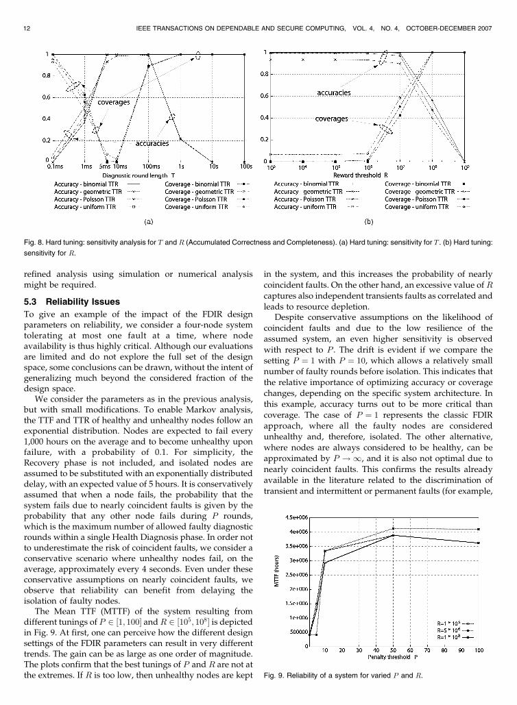
refined analysis using simulation or numerical analysismight be required.

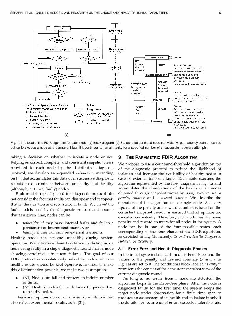
5.3 Reliability Issues

To give an example of the impact of the FDIR designparameters on reliability, we consider a four-node systemtolerating at most one fault at a time, where nodeavailability is thus highly critical. Although our evaluationsare limited and do not explore the full set of the designspace, some conclusions can be drawn, without the intent ofgeneralizing much beyond the considered fraction of thedesign space.

We consider the parameters as in the previous analysis,but with small modifications. To enable Markov analysis,the TTF and TTR of healthy and unhealthy nodes follow anexponential distribution. Nodes are expected to fail every1,000 hours on the average and to become unhealthy uponfailure, with a probability of 0.1. For simplicity, theRecovery phase is not included, and isolated nodes areassumed to be substituted with an exponentially distributeddelay, with an expected value of 5 hours. It is conservativelyassumed that when a node fails, the probability that thesystem fails due to nearly coincident faults is given by theprobability that any other node fails during P rounds,which is the maximum number of allowed faulty diagnosticrounds within a single Health Diagnosis phase. In order notto underestimate the risk of coincident faults, we consider aconservative scenario where unhealthy nodes fail, on theaverage, approximately every 4 seconds. Even under theseconservative assumptions on nearly coincident faults, weobserve that reliability can benefit from delaying theisolation of faulty nodes.

The Mean TTF (MTTF) of the system resulting fromdifferent tunings of P 2 ½1; 100� andR 2 ½105; 108� is depictedin Fig. 9. At first, one can perceive how the different designsettings of the FDIR parameters can result in very differenttrends. The gain can be as large as one order of magnitude.The plots confirm that the best tunings of P and R are not atthe extremes. If R is too low, then unhealthy nodes are kept

in the system, and this increases the probability of nearly

coincident faults. On the other hand, an excessive value of Rcaptures also independent transients faults as correlated andleads to resource depletion.

Despite conservative assumptions on the likelihood ofcoincident faults and due to the low resilience of theassumed system, an even higher sensitivity is observed

with respect to P . The drift is evident if we compare thesetting P ¼ 1 with P ¼ 10, which allows a relatively smallnumber of faulty rounds before isolation. This indicates that

the relative importance of optimizing accuracy or coveragechanges, depending on the specific system architecture. Inthis example, accuracy turns out to be more critical than

coverage. The case of P ¼ 1 represents the classic FDIRapproach, where all the faulty nodes are consideredunhealthy and, therefore, isolated. The other alternative,

where nodes are always considered to be healthy, can beapproximated by P !1, and it is also not optimal due to

nearly coincident faults. This confirms the results alreadyavailable in the literature related to the discrimination oftransient and intermittent or permanent faults (for example,


Fig. 8. Hard tuning: sensitivity analysis for T and R (Accumulated Correctness and Completeness). (a) Hard tuning: sensitivity for T . (b) Hard tuning:

sensitivity for R.

Fig. 9. Reliability of a system for varied P and R.

[20]) and indicates the soundness and correctness of ouranalysis.

These results prove that the FDIR parameters can have aconsiderable impact on the reliability of the system. Byfixing dependability goals (and, hopefully, more detailedgoals for the attributes like safety, reliability, and avail-ability), it is then possible to look for the required levels ofaccuracy, coverage, and latency for a given system. As wehave shown previously, the possibility of finding valuesoptimizing the contrasting attributes depends very much on“external” system parameters, which are not under de-signer control (for example, failure rates), and on otherdesign parameters such as the completeness of the diag-nostic protocol and of its fault assumption, which we didnot specifically address in this work because they are notdirectly related to the count-and-threshold algorithm. Evenif some parameters are not known, we describe next howour framework provides the system designers with techni-ques to study the effect of different design choices under arange of scenarios.

6 PRACTICAL APPLICATION OF THE FDIRFRAMEWORK

Our evaluation approach has been applied to tune twoprototypes, an automotive system and an aerospace system,running on a system implementing our FDIR framework.All requirements and design parameters used during thetuning below arose from actual automotive and aerospaceapplications [29].

During initial implementation, a reasonable thoughapproximate setting of the FDIR parameters was estab-lished, which ensured high coverage of intermittent faults(> 0.999) only, as long as the related expected TTF was inthe order of minutes. Successive use of the tuning processdocumented in this section significantly enhanced the initialsetting. First, the application-level requirements constrain-ing the diagnostic parameters were considered. Next, arange of realistic scenarios were defined in order to tune theunconstrained parameters. Without compromising accu-racy, the new setting extended the range of unhealthy nodesisolated with high likelihood to those failing on the averageas seldom as every 10 hours. This could be done at designtime, as no measurement on the system was needed.

6.1 Application-Specific Design Constraints

In the time-triggered platform used for the implementationall nodes share a common (replicated) broadcast-based bususing a TDMA access scheme. Nodes consist of a host

computer (Infineon Tricore 1796) and a communication

controller (Xilinx Vertex 4 field-programmable gate array

(FPGA)) providing interface to a generic time-triggered

network (layered TTP). Each node is statically assigned a

time window, called sending slot, to broadcast messages to

all other nodes. Nodes are diagnosed based on their

capability of sending messages during the designated

sending slot. Therefore, the diagnostic round length T

equals a time-division multiple access (TDMA) round. Both

considered that safety-critical domains are characterized by

strict application requirements, which define the range of

the feasible parametric settings. The TDMA round (and,

consequently, the diagnostic round) must be short enough

to allow satisfying all the application-level hard real-time

deadlines.The diagnostic protocol is also constrained by require-

ments related to the criticality of different applications. In

automotive systems, multiple criticality classes can be

identified. Safety-Critical (SC) functionalities are necessary

for the physical control of the vehicle with strict reactivity

constraints, for example, X-by-wire. Recovery actions must

be timely and always preserve the availability of the

(possibly degraded) service. Safety-Relevant (SR) functional-

ities support the driver, for example, the Electronic Stability

Control and the Driver Assistant Systems. They are not

necessary for the control of the car, but the driver must know

if these are unavailable. Finally, we considered Non-SR

(NSR) functionalities such as comfort and entertainment

subsystems. In the aerospace prototype, only SC function-

alities are running on the system, for example, the High Lift

system related to the control of flaps and the Landing Gear

system. A summary of the requirements is shown in Table 2.Applications with different criticality classes have

different requirements on the maximum tolerated transient

outage time between the beginning of a faulty burst and the

isolation of the node (and the consequent activation of

recovery actions). As discussed in the previous section,

penalty thresholds greater than 1 increase accuracy and

node availability in the presence of transient faults.

However, during the Health Diagnosis phase of the FDIR

algorithm, an application might be prevented from correctly

exchanging messages if some of its jobs are hosted on a

faulty node that is still kept operative. Therefore, the

maximum tolerated outage represents an upper bound of

the sum of three delays: the detection delay to detect a fault

for the first time, the accumulation delay when faults are

continuously recorded by the diagnostic protocol, but the


TABLE 2Application-Specific Requirements on the Diagnostic Protocol

node is still not isolated, and the recovery delay involved intriggering recovery actions.

The diagnostic protocol operates by detecting if time-triggered messages are delivered correctly and timely. As inthe prototype system, all messages generated by thedifferent jobs of a node are encapsulated into a singlemessage, and the protocol does not discriminate betweenfaults at different services running on the same node. Asingle criticality class, as well as a related penalty incrementpi, is thus assigned to each node according to the toleratedoutage of its highest criticality job.

In the specific setup under consideration, the worst-casedetection delay is four TDMA rounds (10 ms), and localrecovery actions are immediately triggered as soon as anode is consistently isolated. The penalty threshold is firstdefined by considering the class of applications with theleast criticality (NSR). We conservatively considered theshortest tolerated outage associated with the three criticalityclasses identified. In this case, a faulty node must beisolated after bursts of 500 ms. Considering the detectiondelay, the time from detection to isolation must be at most490 ms, which corresponds to 196 diagnostic rounds. Weconsequently set the penalty threshold to P ¼ 196 and thepenalty increment to pNSR ¼ 1. After establishing thepenalty threshold, the penalty increments for applicationclasses with higher criticality can be derived. The maximumnumber of tolerated diagnostic rounds for the other twocriticality classes ðtolfSC;SRgÞ can be similarly calculated bysubtracting the detection delay from the tolerated outage.The penalty increments must ensure that the penaltythreshold P is reached within tolfSC;SRg diagnostic rounds,that is, pfSC;SRg ¼ dP � T=tolfSC;SRge. It is remarkable that theresulting values reported in Table 2 are just slightly moreconservative than the values experimentally identified in[29], reflecting our conservative assumptions.

6.2 Characterization of the System

Our tuning process allows evaluation of accuracy andcoverage levels resulting from different parametric settingsof the FDIR process. In our case study, P , T , and the penaltyincrements are constrained by domain-specific require-ments. We are thus interested in setting R in order tocorrelate the largest range of intermittent faults whileavoiding an excessive reduction of accuracy due tocorrelation of successive external transient faults.

The tuning process requires three input parametersrelated to the system: the TTR of all nodes, the (transient)TTF of healthy nodes, and the (intermittent) TTF ofunhealthy nodes. These values can be known fromstandards, expertise, or literature. When precise values arenot available, a range of reasonable scenarios must beexamined for sensitivity analysis.

The transient TTF for different classes of faults andoperational conditions has been extensively studied andsometimes included in standards (see [20] for a survey onpublished rates for different types of faults that are typicalof embedded systems). Reported values are all well below arate of 10�3 faults=h. In our case, we considered twoconservative rates of 10�2 and 10�3 faults=h to account forthe foreseen trend toward higher rates [9]. The TTF forintermittent faults is system specific and it depends on

multiple factors such as the specific component beingdamaged or the activation patterns of the software. As aresult, this value is unknown in most practical systems.Therefore, we consider an intermittent TTF following aWeibull distribution, with � ¼ 1:4 [31], and expected valuesranging ½1 minute� 100 hours�. Regarding the expectedTTR, safety-critical systems are often validated by injectingtemporary faults and observing the capability of the systemto tolerate them. Such tests are supposed to represent real-world operational conditions. According to the Interna-tional Organization for Standardization (ISO) 7637 testingstandard for the automotive domain [14], we considered anexpected TTR of 5 ms, which is also a reasonable value forthe aerospace domain.

6.3 Tuning the System to Improve Coverage

The defined scenarios were used to study the coverage andaccuracy levels for the three criticality classes with respectto different tunings of R and to determine 1) how large Rcan be set before accuracy is compromised and 2) what thelargest expected TTF for intermittent faults resulting in highlevels of coverage is.

The value R ¼ 106 was chosen as the first setting in thecontext of the experimental validation of the protocol [29],as it appeared as a good practical trade-off. In fact, it allowscorrelating all intermittent faults appearing within a timewindow R � T ffi 42 minutes, whereas two distinct transientfaults are incorrectly correlated with a probability lowerthan 1 percent in the scenarios that we considered. In thefollowing, we show that a better tuning can be found bymeans of a more extensive probabilistic evaluation.

The plots of accuracy and coverage for the three severityclasses are depicted in Fig. 10 and were obtained using thesimple closed-form expression of (2). Besides the fact thatthe main trends are consistent with those identified in theprevious section, some interesting aspects specific to theapplication domains under consideration emerge. Asexpected, nodes with higher criticality display better cover-age and worse accuracy.

The value selected during the experimental evaluation ofthe protocol R ¼ 106 ensures a very high level of accuracy(above 0.98) for all criticality classes and transient faultrates. Unhealthy nodes are isolated with high coverage iftheir expected TTF is in the order of minutes. For largerexpected TTF (greater than 1 hour) isolation is unlikely evenif SC nodes are impacted.

In general, we observe that by tuning of R � 108, alevel of accuracy above 0.97 can be reached for allcriticalities, the sole exception being the case of SC nodeswith the conservative transient TTF of 100 hours. In thiscase, accuracy drops to around 0.78. On the other hand,settings of R � 108 result in high coverage (above 0.9996)for all criticalities classes and for expected intermittentTTF � 10 hours.

Such tuning highlights that a better setting of R ¼ 108

exists, which significantly improves coverage withoutimpacting accuracy, especially if the transient TTF can besafely assumed to be more than 1,000 hours. Due to morerestrictive requirements on the maximum tolerated outage,SC nodes are more likely subject to wrong isolations(especially under adverse external conditions when external


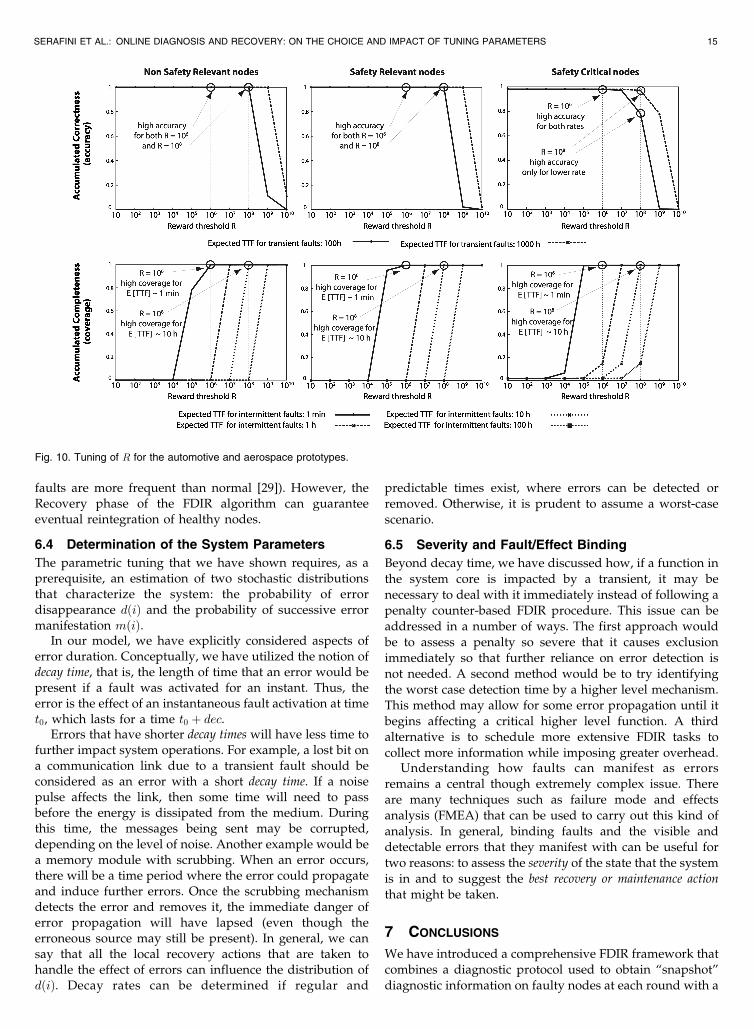
faults are more frequent than normal [29]). However, theRecovery phase of the FDIR algorithm can guaranteeeventual reintegration of healthy nodes.

6.4 Determination of the System Parameters

The parametric tuning that we have shown requires, as aprerequisite, an estimation of two stochastic distributionsthat characterize the system: the probability of errordisappearance dðiÞ and the probability of successive errormanifestation mðiÞ.

In our model, we have explicitly considered aspects oferror duration. Conceptually, we have utilized the notion ofdecay time, that is, the length of time that an error would bepresent if a fault was activated for an instant. Thus, theerror is the effect of an instantaneous fault activation at timet0, which lasts for a time t0 þ dec.

Errors that have shorter decay times will have less time tofurther impact system operations. For example, a lost bit ona communication link due to a transient fault should beconsidered as an error with a short decay time. If a noisepulse affects the link, then some time will need to passbefore the energy is dissipated from the medium. Duringthis time, the messages being sent may be corrupted,depending on the level of noise. Another example would bea memory module with scrubbing. When an error occurs,there will be a time period where the error could propagateand induce further errors. Once the scrubbing mechanismdetects the error and removes it, the immediate danger oferror propagation will have lapsed (even though theerroneous source may still be present). In general, we cansay that all the local recovery actions that are taken tohandle the effect of errors can influence the distribution ofdðiÞ. Decay rates can be determined if regular and

predictable times exist, where errors can be detected orremoved. Otherwise, it is prudent to assume a worst-casescenario.

6.5 Severity and Fault/Effect Binding

Beyond decay time, we have discussed how, if a function inthe system core is impacted by a transient, it may benecessary to deal with it immediately instead of following apenalty counter-based FDIR procedure. This issue can beaddressed in a number of ways. The first approach wouldbe to assess a penalty so severe that it causes exclusionimmediately so that further reliance on error detection isnot needed. A second method would be to try identifyingthe worst case detection time by a higher level mechanism.This method may allow for some error propagation until itbegins affecting a critical higher level function. A thirdalternative is to schedule more extensive FDIR tasks tocollect more information while imposing greater overhead.

Understanding how faults can manifest as errorsremains a central though extremely complex issue. Thereare many techniques such as failure mode and effectsanalysis (FMEA) that can be used to carry out this kind ofanalysis. In general, binding faults and the visible anddetectable errors that they manifest with can be useful fortwo reasons: to assess the severity of the state that the systemis in and to suggest the best recovery or maintenance action

that might be taken.

7 CONCLUSIONS

We have introduced a comprehensive FDIR framework thatcombines a diagnostic protocol used to obtain “snapshot”diagnostic information on faulty nodes at each round with a


Fig. 10. Tuning of R for the automotive and aerospace prototypes.

count-and-threshold algorithm, which accumulates thisinformation, to produce a health assessment of the nodestaking transient faults of varied duration explicitly intoaccount. The FDIR framework also details the recoveryphase of a system as an organic part of the diagnosticprocess, considers the definition of varied severity classes,and makes proposals for their management.

This work has made contributions in 1) determining andestablishing the effect of the duration and recurrence oferrors on the effectiveness of online diagnosis protocols,2) ascertaining the sensitivity and the trade-offs involvingsome FDIR design parameters in determining the correct-ness and completeness of the FDIR protocols and inimproving system reliability, and 3) describing an applica-tion of the approach on two practical systems.

By developing a generic and comprehensive analyticframework, we have been able to provide methods to guideand ease the tuning of the parameters. We have shown thatdesign parameters such as the diagnostic round length,which influences the performance of the system, can alsoconsiderably impact the system reliability and task-orientedavailability. Thus, depending on the failure modes expectedin a particular environment, the system designer canoptimize the FDIR algorithm to minimize wrong isolationswith the increased task-oriented availability of the system.We identified the main trends by means of a sensitivitystudy, varying the different FDIR parameters withinreasonable bounds. Finally, we have shown the practicalityof the approach by implementing and tuning it onto twoprototypes for automotive and aerospace applications,addressing open issues such as the determination of properseverity levels for different classes of errors. Withoutviolating any application-level constraints, the achievedprobability of node isolation due to transient faults is almostnegligible, whereas nodes with internal dormant faults areisolated, even if errors appear as seldom as every 10 hours.

APPENDIX

In this section, we solve the DTCM of Fig. 3 and obtain theresult of (2).

Theorem. Consider an FDIR process with penalty threshold P ,reward threshold R, diagnostic round length T , and unarypenalty increments. If a node with a constant disappearancehazard dðiÞ ¼ d and reappearance hazard mðiÞ enters theHealth Diagnosis phase, then it is isolated with a probability:

Pisol ¼ 1� d �YR�1

i¼1


:

Proof. We solve the chain by adding to it two dummytransitions having probability 1 from the absorbing statesto the initial state h1; 0i, thus modeling an infinitenumber of execution of the Health Diagnosis after anerror appears, and solving the new irreducible model atthe steady state. If the time-averaged steady stateprobability of the states “Isolated” and “Reset” are,respectively, �I and �R, then we can derive Pisol as

Pisol ¼�I

�I þ �R: ð3Þ

Assuming that �p;r represents the time-averagedsteady state probability of state hp; ri, the flow equationsfor the Markov chain are given by

�1;0 ¼ �I þ �R; ð4Þ

�p;0 ¼ ð1� dÞ�p�1;0 þXR�1

r¼1

mðrÞ�p�1;r; ð5Þ

�I ¼ ð1� dÞ�P�1;0 þXR�1

r¼1

mðrÞ�P�1;r; ð6Þ

�p;1 ¼ d�p;0; ð7Þ

�p;r ¼ ð1�mðr� 1ÞÞ�p;r�1; ð8Þ

�R ¼XP�1

p¼1

ð1�mðR� 1ÞÞ�p;R�1: ð9Þ

Unfolding (8), we have

�p;r ¼Yr�1

i¼1

ð1�mðiÞÞ�p;1:

From (7) and by substituting �p:r in (5), we have

�p;0 ¼ 1� dþ dXR�1

r¼1

mðrÞYr�1

i¼1

ð1�mðiÞÞ !

�p�1;0:

From the definition of mðkÞ as the discrete hazard

function of fbY ðkÞ, it follows that

1�mðiÞ ¼1� FbY ðiÞ

1� FbY ði� 1Þ ;Yr�1

i¼1

1�mðiÞ ¼ 1� FbY ðr� 1Þ;

mðrÞYr�1

i¼1

1�mðiÞ ¼ fbY ðrÞ:Therefore,

�p;0 ¼ð1� dþ dXR�1

r¼1

fbY ðrÞÞ�p�1;0;

¼ð1� dð1� FbY ðR� 1ÞÞÞ�p�1;0;

¼ 1� dYR�1

i¼1

ð1�mðiÞÞ !

�p�1;0:

Unfolding and from (6), we have

�p;0 ¼ 1� dYR�1

i¼1

ð1�mðiÞÞ !ðp�1Þ

�1;0;

�I ¼ 1� dYR�1

i¼1


�1;0:


Using �1:0 from (4), we can derive Pisol from (3):

�I ¼ 1� dYR�1

i¼1


ð�I þ �RÞ;

Pisol ¼ 1� dYR�1

i¼1


:

tu

ACKNOWLEDGMENTS

The research of Marco Serafini and Neeraj Suri has beensupported in part by the European Commission Depend-able Embedded Components and Systems (EC DECOS),Resilience for Survivability in IST (ReSIST), and DeutscheForschungsgemeinschaft Technische Universitat DarmstadtCooperative, Adaptive and Responsive Monitoring inMixed Mode Systems (DFG TUD GKMM). The authorsare grateful to the entire Dependable, Embedded Systemsand Software (DEEDS) Group, TUD, for their inputs andhelp.

REFERENCES

[1] P. Agrawal, “Fault Tolerance in Multiprocessor Systems withoutDedicated Redundancy,” IEEE Trans. Computers, vol. 37, no. 3,pp. 358-362, Mar. 1988.

[2] M. Barborak, M. Malek, and A. Dahbura, “The ConsensusProblem in Fault-Tolerant Computing,” ACM Surveys, vol. 25,no. 2, pp. 171-220, June 1993.

[3] K. Birman and T. Joseph, “Exploiting Virtual Synchrony inDistributed Systems,” Proc. 11th Symp. Operating Systems Principles(SOSP ’87), pp. 123-138, 1987.

[4] D.M. Blough and H.W. Brown, “The Broadcast ComparisonModel for On-Line Fault Diagnosis in Multicomputer Systems:Theory and Implementation,” IEEE Trans. Computers, vol. 48,no. 5, pp. 470-493, May 1999.

[5] M. Blount, “Probabilistic Treatment of Diagnosis in DigitalSystems,” Proc. Seventh Ann. Int’l Symp. Fault-Tolerant Computing(FTCS ’77), pp. 72-77, 1977.

[6] A. Bondavalli, S. Chiaradonna, F. Di Giandomenico, and F.Grandoni, “Discriminating Fault Rate and Persistency to ImproveFault Treatment,” Proc. 27th Ann. Int’l Symp. Fault-TolerantComputing Symp. (FTCS ’97), pp. 354-362, 1997.

[7] A. Bondavalli, S. Chiaradonna, F. Di Giandomenico, and F.Grandoni, “Threshold-Based Mechanisms to Discriminate Tran-sient from Intermittent Faults,” IEEE Trans. Computers, vol. 49,no. 3, pp. 230-245, Mar. 2000.

[8] T. Chandra and S. Toueg, “Unreliable Failure Detectors forReliable Distributed Systems,” J. ACM, vol. 43, no. 2, pp. 225-267, Mar. 1996.

[9] C. Constantinescu, “Impact of Deep Submicron Technology onDependability of VLSI Circuits,” Proc. IEEE Int’l Conf. DependableSystems and Networks (DSN ’02), pp. 205-209, 2002.

[10] F. Cristian, “Reaching Agreement on Processor-Group Member-ship in Synchronous Distributed Systems,” Distributed Computing,vol. 4, no. 4, pp. 175-187, Dec. 1991.

[11] F. Cristian and C. Fetzer, “The Timed Asynchronous DistributedSystem Model,” IEEE Trans. Parallel and Distributed Systems,vol. 10, no. 6, pp. 642-657, June 1999.

[12] D.D. Deavours, G. Clark, T. Courtney, D. Daly, S. Derisavi, J.M.Doyle, and W.H. Sanders, “The Mobius Framework and ItsImplementation,” IEEE Trans. Software Eng., vol. 20, no. 10,pp. 956-969, Oct. 2002.

[13] L. Gong, P. Lincoln, and J. Rushby, “Byzantine Agreement withAuthentication: Observations and Applications in ToleratingHybrid and Link Faults,” Proc. Fifth Conf. Dependable Computingfor Critical Applications (DCCA ’95), pp. 139-157, 1995.

[14] “Road Vehicles—Electrical Disturbances from Conduction andCoupling” ISO 7637, Int’l Organization for Standardization, 1997.

[15] R. Iyer, L.T. Young, and P.V.K. Iyer, “Automatic Recognition ofIntermittent Failures: An Experimental Study of Field Data,” IEEETrans. Computers, vol. 39, no. 3, pp. 525-537, Apr. 1990.

[16] H. Kopetz and G. Grunsteidl, “TTP—A Protocol for Fault-TolerantReal-Time Systems,” Computer, vol. 27, no. 1, pp. 14-23, Jan. 1994.

[17] J. Kuhl and S. Reddy, “Fault Diagnosis in Fully DistributedSystems,” Proc. 11th Ann. Int’l Symp. Fault-Tolerant Computing(FTCS ’81), pp. 100-105, 1981.

[18] J. Lala and L. Alger, “Hardware and Software Fault Tolerance: AUnified Architectural Approach,” Proc. 18th Ann. Int’l Symp. Fault-Tolerant Computing (FTCS ’88), pp. 240-245, 1988.

[19] J.-C. Laprie, “Dependable Computing and Fault Tolerance:Concepts and Terminology,” Proc. 25th Ann. Int’l Symp. Fault-Tolerant Computing (FTCS ’95), pp. 2-11, 1995.

[20] E. Latronico and P. Koopman, “Design Time Reliability Analysisof Distributed Fault Tolerance Algorithms,” Proc. IEEE Int’l Conf.Dependable Systems and Networks (DSN), pp. 486-495, 2005.

[21] T. Lin and D. Siewiorek, “Error Log Analysis: Statistical Modelingand Heuristic Trend Analysis,” IEEE Trans. Computers, vol. 39,no. 4, pp. 419-432, Oct. 1990.

[22] P. Lincoln and J. Rushby, “A Formally Verified Algorithm forInteractive Consistency under a Hybrid Fault Model,” Proc. 23rdAnn. Int’l Symp. Fault-Tolerant Computing (FTCS ’93), pp. 402-411,1993.

[23] S. Mallela and G. Masson, “Diagnosis without Repair for HybridFault Situations,” IEEE Trans. Computers, vol. 29, no. 6, pp. 461-470,June 1980.

[24] M. Malek, “A Comparison Connection Assignment for Diagnosisof Multiprocessor Systems,” Proc. Seventh Ann. Symp. ComputerArchitecture, pp. 31-36, 1980.

[25] D. Powell, J. Arlat, L. Beus-Dukic, A. Bondavalli, P. Coppola, A.Fantechi, E. Jenn, C. Rabejac, and A. Wellings, “GUARDS: AGeneric Upgradable Architecture for Real-Time DependableSystems,” IEEE Trans. Parallel and Distributed Systems, vol. 10,no. 6, pp. 580-599, June 1999.

[26] F.P. Preparata, G. Metze, and R.T. Chien, “On the ConnectionAssignment Problem of Diagnosable Systems,” IEEE Trans.Electronic Computers, vol. 16, no. 12, pp. 848-854, Dec. 1967.

[27] U. Schmid, “How to Model Link Failures: A Perception-BasedFault Model,” Proc. Int’l Conf. Dependable Systems and Networks(DSN ’95), pp. 57-66, 1995.

[28] A. Sengupta and A. Dahbura, “On Self-Diagnosable Multi-processor Systems: Diagnosis by the Comparison Approach,”IEEE Trans. Computers, vol. 41, no. 11, pp. 1386-1396, Nov. 1992.

[29] M. Serafini, N. Suri, J. Vinter, A. Ademaj, W. Brandstatter, F.Tagliabo, and J. Koch, “A Tunable Add-On Diagnostic Protocolfor Time-Triggered Systems,” Proc. Int’l Conf. Dependable Systemsand Networks (DSN ’07), pp. 164-174, 2007.

[30] K. Shin and P. Ramanathan, “Diagnosis of Processors withByzantine Faults in a Distributed Computing System,” Proc. 17thAnn. Int’l Symp. Fault-Tolerant Computing (FTCS ’87), pp. 55-60,1987.

[31] D.P. Siewiorek and R.R. Swarz, Reliable Computer Systems: Designand Evaluation. AK Peters, 1998.

[32] C. Walter, M.M. Hugue, and N. Suri, “Continual On-LineDiagnosis of Hybrid Faults,” Proc. Fourth Conf. DependableComputing for Critical Applications (DCCA ’94), pp. 150-166, 1994.

[33] C. Walter, P. Lincoln, and N. Suri, “Formally Verified On-LineDiagnosis,” IEEE Trans. Software Eng., vol. 23, no. 11, pp. 684-721,Nov. 1997.


Marco Serafini received the Laurea degree(summa cum laude) from the University ofFlorence, Italy. He is currently working towardthe PhD degree at the Technische UniversitatDarmstadt, Darmstadt, Germany. His researchinterests include dependable distributed sys-tems, in particular online monitoring, fault loca-tion, and failure model characterization. Hecoordinates the diagnostic activities of theEuropean Union Dependable Embedded Com-

ponents and Systems (EU DECOS) Project. He is also currentlycollaborating with Hitachi on the design, verification, and experimentalvalidation of safety-critical middleware for generic time-triggeredsystems. He is a student member of the IEEE and the IEEE ComputerSociety.

Andrea Bondavalli (M’96) is a professor inthe Department of Systems and Informatics,University of Florence, Italy. Previously, hewas a researcher at the Italian NationalResearch Council, working at the CNUCEInstitute, Pisa, where he was responsible forthe Dependable Computing Group. He hasbeen the principal investigator (PI) in manyprojects funded by the European Community,currently IST-2004-26979 HIDENETS and

2005-31413 SAFEDMI, acted in several occasions as an expert forthe European community, and served as the program chair of themost important conferences in the area, including the 2005 Depend-able Computing and Communications Symposium—The InternationalConference on Dependable Systems and Networks (DCC-DSN), the19th IEEE Symposium on Reliable Distributed Systems (SRDS ’00),the 2002 European Dependable Computing Conference (EDCC-4),the Third Latin-American Symposium on Dependable Computing(LADC ’07). He is a member of the International Federation forInformation Processing (IFIP) Working Group 10.4 on “DependableComputing and Fault-Tolerance,” European Network of Clubs forReliability and Safety of Software intensive systems (ENCRESS)Club, Italy, and the AICA Working Group on Dependability inComputer Systems. His research activities and interests are thedesign and validation of critical systems and infrastructures, inparticular the design of fault-tolerant architectures, mechanisms, andprotocols, as well as their evaluation in terms of dependabilityattributes such as reliability, availability, and performability. He is theauthor of more than 110 refereed publications in international journalsand conference proceedings. He is a member of the IEEE and theIEEE Computer Society.

Neeraj Suri received the PhD degree from theUniversity of Massachusetts, Amherst. He iscurrently the chair professor of the DependableEmbedded Systems and Software Group,Technische Universitat Darmstadt, Darmstadt,Germany. His earlier academic appointmentsinclude the Saab endowed professorship andfaculty member at Boston University. He is amember of the International Federation forInformation Processing (IFIP) Working Group

10.4 on Dependability and Microsoft’s Trustworthy Computing Aca-demic Advisory Board. He has served as the program committee (PC)chair for the IEEE Symposium on Reliable Distributed Systems(SRDS), the IEEE International Symposium on High AssuranceSystems Engineering (HASE), the International Service AvailabilitySymposium (ISAS), and Microsoft-TUD RAF and will serve as the PCChair for the upcoming 2008 Dependable Computing and Commu-nications Symposium—The International Conference on DependableSystems and Networks (DCC-DSN). His research interests include thedesign, analysis, and assessment of dependable and secure systems,software, and services. His group’s research activities have garneredsupport from the European Commission, the US Defense AdvancedResearch Projects Agency (DARPA), Deutsche Forschungsge-meinschaft (DFG), the US National Science Foundation (NSF),NASA, the Naval Air Warfare Center (NAWC), the US Office ofNaval Research (ONR), Boeing, Microsoft, Intel, Saab, and Hitachiamong others. He is an associate editor of the IEEE Transactions onDependable and Secure Computing, the IEEE Transactions onSoftware Engineering, the ACM Computing Surveys, and theInternational Journal of Security and Networks and has been anassociate editor of the IEEE Transactions on Parallel and DistributedSystems. He is also a recipient of an US NSF Faculty Early CareerDevelopment (CAREER) award. He is a senior member of the IEEEand the IEEE Computer Society.

. For more information on this or any other computing topic,please visit our Digital Library at www.computer.org/publications/dlib.


ieee transactions on dependable and secure …tdsc07.pdf · the first approaches to group...

Documents