ieee transactions on parallel and distributed...

1045-9219 (c) 2013 IEEE. Personal use is permitted, but republication/redistribution requires IEEE permission. Seehttp://www.ieee.org/publications_standards/publications/rights/index.html for more information.

This article has been accepted for publication in a future issue of this journal, but has not been fully edited. Content may change prior to final publication. Citationinformation: DOI 10.1109/TPDS.2014.2345257, IEEE Transactions on Parallel and Distributed Systems

IEEE TRANSACTIONS ON PARALLEL AND DISTRIBUTED SYSTEMS, VOL.X , NO.X , XXXX 201X 1

CDC: Compressive Data Collection forWireless Sensor Networks

Xiao-Yang Liu, Yanmin Zhu, IEEE Member , Linghe Kong, IEEE Member , Cong Liu,Yu Gu, IEEE Member , Athanasios V. Vasilakos, IEEE Senior Member ,

Min-You Wu, IEEE Senior Member

Abstract—Data collection is a crucial operation in wireless sensor networks. The design of data collection schemes ischallenging due to the limited energy supply and the hot spot problem. Leveraging empirical observations that sensory datapossess strong spatiotemporal compressibility, this paper proposes a novel compressive data collection scheme for wirelesssensor networks. We adopt a power-law decaying data model verified by real data sets and then propose a random projection-based estimation algorithm for this data model. Our scheme requires fewer compressed measurements, thus greatly reduces theenergy consumption. It allows simple routing strategy without much computation and control overheads, which leads to strongrobustness in practical applications. Analytically, we prove that it achieves the optimal estimation error bound. Evaluations onreal data sets (from the GreenOrbs, IntelLab and NBDC-CTD projects) show that compared with existing approaches, this newscheme prolongs the network lifetime by 1.5× to 2× for estimation error 5% ∼ 20%.

Index Terms—Compressive Data Collection, Wireless Sensor Networks, Compressive Sensing, Random Compression, Nonuni-form Random Projection

F

1 INTRODUCTION

W IRELESS sensor networks (WSNs) are adopt-ed in many military, civilian and commercial

applications recent years [1]. A crucial operation ofWSNs [2] is to perform data collection, where sensorreadings are collected from sensor nodes and thentransmitted to the sink through multi-hop wirelesscommunications. Various applications rely on effi-cient data collection, such as battlefield surveillance[3][4][5], habit monitoring [6], infrastructure monitor-ing [7], and environmental monitoring [8].

A primary challenge of designing data collectionschemes lies in prolonging the network lifetime. First-ly, each sensor node, being a micro-electronic device,can only be equipped with a limited power sourcewhile in many applications, recharging is impractical(impossible or not worth it). Thus, a WSN can onlysupport limited volume of traffic load. Secondly, theinformation that a WSN can effectively transport iseven less under multi-hop transmissions since thenetwork capacity decreases as the number of nodesincreases [9], i.e., the multi-hop scheme requires lotsof packet forwardings. Thirdly, the many-to-one trafficpattern, called convergecast [10], of data collection in-duces load unbalance. It leads to the hot spot problem[11], i.e., the sensor nodes closer to the sink will run

• Xiao-Yang Liu, Yanmin Zhu, Linghe Kong and Min-You Wu are withShanghai Jiao Tong University, China. Cong Liu is with Universityof Texas at Dallas, USA. Yu Gu is with Singapore University ofTechnology and Design, Singapore. Athanasios V. Vasilakos is withUniversity of Western Macedonia, Greece. Linghe Kong is the corre-sponding author ([email protected]).

out of energy sooner. Therefore, the network lifetimeof WSNs will be significantly shortened.

Furthermore, designers have to deal with the fol-lowing constraints: the unreliability of low-powerwireless communication, and the limited computa-tional ability of sensor nodes. Low-power transceiversinduce poor link quality, therefore packet loss occursfrequently [12][13]. Actually, real-world WSN projectssuffer from serious data loss with loss rates as high as23% ∼ 64% [12]. To ensure reliable transmission willcost unconscionable amount of energy as it induces anexceptionally huge number of retransmissions, whichis not cost-effective. On the other hand, sensor nodescan only support simple computing tasks, thereforethe preprocessing or compression of data collectionschemes should be easy to implement.

Existing solutions have limitations and thus areunsatisfactory. Generally, data collection in WSNsfollows two approaches: raw-data collection andaggregated-data collection. WSNs are typically com-posed of hundreds to thousands of sensor nodesgenerating tremendous amount of sensory readings,as the packet loss problem and the hot spot problemsurface, raw-data collection is rather inefficient orproblematic [11][13]. This approach will lead to alarge number of retransmissions in real-world situa-tions and node failures (cluster headers, or tree node,etc.) as batteries run out. Aggregated-data collectiontakes advantage of spatiotemporal correlations (orcompressibility) within sensory data to reduce com-munication costs. More specifically, in-network datacompression [14] is adopted to reduce global traffic,such as distributed source coding [15] or transform




coding [16]. However, they incur significant compu-tation and control overheads, i.e., the former onerelies on communications between neighbor nodes,while the later one requires complicated transformingcomputation, which are not suitable for WSNs.

Compressive sensing theory [17][18] exhibits suc-cessful application in designing effective data collec-tions [11][19]. The authors in [11] propose a com-pressive data gathering (CDG) scheme which re-duces global-scale communication costs while achiev-ing tempting load balancing. However, it assumesa perfectly reliable routing tree, thus is vulnerableto packet loss or node malfunctioning. Maintainingsuch routing infrastructure will cause large controloverheads. Although in simulations it behaves wellunder careful controls, the practical performance isunsatisfactory.

Main Contributions: Firstly, we propose a novelcompressive data collection scheme for wireless sen-sor networks. Our scheme compresses sensory read-ings “on the fly” under an opportunistic routing.

Secondly, we model the data collection process asa nonuniform sparse random projection (NSRP), wepropose a NSRP-based estimator which guaranteesoptimal error bound.

Finally, based on real data sets, we show that ourscheme prolongs the network lifetime by 1.5× to 2×for estimation error 5% ∼ 20%, compared with thebaseline scheme and the CDG [11] scheme.

2 RELATED WORK

Energy conservation [20] is an important issue inwireless sensor networks. In-network compressionis a promising approach to reduce the amount ofinformation to be transmitted by exploiting sensorydata’s redundancy. We classified existing data collec-tion schemes into three categories: conventional com-pression, distributed source coding, and compressivesensing.

Conventional compression. Conventional compres-sion techniques assume specific data structures andthus require communication among sensor nodes [20].In joint entropy coding approach, nodes use relayeddata as side information to encode their readings. Ifthe data are allowed to be communicated back andforth during encoding, sensor nodes may coopera-tively perform transforms to better utilize the cor-relation, such as the gossip-based technique used in[19]. There are two main problems with this approach.First, the route heavily influences the compressionperformance [14]. To achieve high compression ratio,data compression and packet routing are required tobe optimized jointly, which is proved to be NP-hard[21][22]. Second, structure-aware data compressioninduces computational and communication overheads[14][23][24], rendering this kind of data collectionschemes to be inefficient.

Distributed source coding. Distributed source cod-ing intends to reduce complexity at sensor nodes andto utilize correlation at the sink [15]. After encod-ing sensor readings independently, each node simplysends the compressed message along the shortest pathto the sink [8]. Distributed source coding performswell for static correlation patterns. However, whencorrelation pattern changes or anomaly readings showup, the estimation accuracy will be greatly affected.

Compressive sensing: Recently, compressive sensinggains increasing attention in wireless sensor networks[16][19][11]. In both static and mobile sensor net-works [23], the interplay of routing with compressivesensing is a key issue [25]. Some of them concludethat although sparsity exists in the environment, therestricted isometry property (RIP) is required by tradi-tional compressive sensing decoder, and hardly goodapproximations can be achieved. Then some proposednetwork-layer compression [26] to avoid this kind ofproblem. Our scheme adopts opportunistic routingwith quite simple compression, therefore the datacollection process is dynamic. This dynamic featureleads to energy balancing and finally benefits energyconsumption.

Note that there are several solvers that are relat-ed with our work. Actually, all compressive sensingsolvers are designed for random projections. Few ofthem use sparse random projections [26][27]. Ourwork are motivated by [26], however, that solvercannot be applied directly for wireless sensor net-works since uniform sampling is hard to achieve andthus will require complicated control overhead. Beliefpropagation [27] exploits sparse encoding, however italso works for uniform sampling while our estimatoris the first solver that can deal with nonuniformsampling. The probability distribution is also usedin their decoding process, which is treated as priorinformation while we use the sampling distributionin the generation of a projection matrix for decoding.

3 SYSTEM MODEL AND DESIGN OVERVIEW

3.1 Network ModelWe consider a wireless sensor network consisting of nsensor nodes and a sink. Sensor nodes are distributedin the target field to sense the physical conditions andthen report sensory readings back to the sink throughmulti-hop transmissions.

Since wireless sensor networks use low-powertransceivers, the link quality is bad, as revealed in[12][13]. We assume that the wireless channel is lossy.It is the motivation of adopting the opportunisticrouting in Section 4.1.

The monitoring period is evenly divided into Ttime slots, denoted as 0, 1, ..., t, ..., T − 1. A recordat the sensor node includes sensor reading, node ID,position (longitude and latitude), and time stamp. Theformat of a record is:




Let Ui,t denote the sensor reading of the i-th node atslot t, which may be temperature, humidity, illumina-tion, etc. Then, a physical condition, say temperature,can be represented as a data matrix:

U =

U0,0 ... U0,t ... U0,T−1

U1,0 ... U1,t ... U1,T−1

... ... ... ...Un−1,0 ... Un−1,t ... Un−1,T−1

, (1)

where the i-th row is the i-th node’s reading sequence,and the t-th column is the whole network’s readingsat slot t.

Notations: U refers to either a matrix or a vec-tor, depending on the context; throughout the paper,N = n× T ; UT is the transpose of U ; |θ| denotes themagnitude of coefficient θ; ∥U∥2 is the ℓ2 normal of U ;Ψ denotes the transform basis. A packet at the sinkis called a measurement throughout the paper.

3.2 Data ModelWe consider a data vector U ∈ RN×1, and an orthonor-mal transform Ψ = [Ψ1,Ψ2, ...,ΨN ] ∈ RN×N . Ψ canbe a wavelet or a Fourier transform basis [28]. Thecoefficients vector θ = [Ψ1U,Ψ2U, ...,ΨNU ]T can bereordered decreasingly in terms of magnitude, suchthat |θ|(1) ≥ |θ|(2) ≥ ... ≥ |θ|(N).

Power-law Decaying Data Model. The coefficients’magnitude decays according to the power law [29],i.e., the i-th largest coefficient satisfies

|θ|(i) ≤ Ci−1/ϖ, i = 1, 2, ..., n, (2)

where C is a constant and −1/ϖ controls the com-pressibility of the data.

Optimal Error Bound. The optimal approximationfor the power-law decaying data [29] is keeping thelargest K coefficients and setting the others as zero.The optimal estimation error bound is:

∥U − Uopt∥22 = ∥θ − θopt∥22 = ηϖCK−1/ϖ+1/2, (3)

where ηϖ is a constant that only depends on −1/ϖ.We verify this data model based on the data set list-

ed in Table 1. Please refer to our online supplementaryfile. Note that our estimator in Section 4.5 is robust tonoise, which is an inherent capability from the abovedata model. However, our model cannot deal withanomaly readings (sensor faults and outliers).

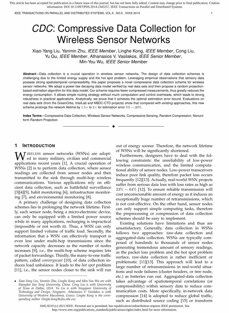
3.3 Design OverviewThe framework of our scheme is shown in Fig.1. Ithas two major components: an opportunistic rout-ing and an estimator. The opportunistic routing isresponsible for data compression and packet relaying.By modeling it as a Markov chain, the compressionprobability of each node can be calculated. Then,

record: reading ID position time stamp

U V θ

V θ

=U: data vector

Y

W

V: transform basis

θ: coefficients

Y: measurements

V : projected basis

θ: estimated coefficients

: transforming

=

M

W: compression vectorM: projection vector

Fig. 1. The framework of CDC.

we prove that nonuniform sparse random projection(NSRP) preserves inner product of two vectors andapply this property to design a simple but quiteaccurate estimator.

At the beginning, data U (θ = UT V ) is stored locallyin sensor nodes. Each sensor node generates a TOKENwith probability p. Therefore, initially there are L = np(in expectation) TOKENs across the network.

The compressive data collection scheme works inthe following way:

• Each node with a TOKEN generates one packetdestinationed to the sink.

• The packets are relayed under an opportunisticrouting. Compression is performed at each newlyencountered node.

• At the sink, the compression process is modelledas YL×1 = WL×NUN×1. Projecting the basis V byM , we have V ′. Then, θ = Y T V ′ is an estimationof θ.

• Finally, U = (θV −1)T , where V −1 is the inverseof V .

Key Issues:• How to determine p? Since p = L/n while n is

known, we will show how to determine L.• The classic result of linear algebra says that θ =

Y T V ′ is solvable only when L ≥ N . To makethe data collection efficient, we are faced withthe question: how to exploit the compressibilityof sensory data by designing an estimation algo-rithm for the case L ≪ N . Compressive sensingtheory [17][18] points out that this is possible.

In Section 4, we first describe how our data collec-tion scheme works and then model it mathematically.Finally, an estimator and the corresponding results forL are presented in Section 4.5.

4 DESIGN

4.1 Opportunistic Routing with CompressionThe opportunistic routing has two tasks: packet for-warding and data compression. We first describe adata collection path, and then the compression processalong this path.

Packet ForwardingFor node si, we define a nearer-to-sink neighbor set as

the one-hop neighbors that are closer to the sink thanitself, i.e., N (i) = j|d(j, sink) ≤ d(i, sink) & d(i, j) ≤Rc where Rc is the communication range. When a




packet arrives at node si, si compresses its sensoryreading into the packet and then sends it out ac-cording to the opportunistic routing [30][31][32], i.e.,forwarding the packet to a randomly selected one ofits nearer-to-sink neighbors sj ∈ N (i). In this way,each packet is guaranteed to be successfully deliveredto the sink.

Data Collection PathThe trajectory of the l-th packet from a source node

to the sink is called a data collection path, denoted asPl = ⟨p0, p1, ..., pρl

⟩ with pρl= sink, i.e., the packet

travels across ρl sensor nodes before it reaches thesink.

Since opportunistic routing is adopted, the datacollection paths are dynamic and random. It turns outto bring about two good features: energy balancingand security. These non-deterministic data collectionpaths will balance energy consumption among nodes,as well as preventing possible attacks.

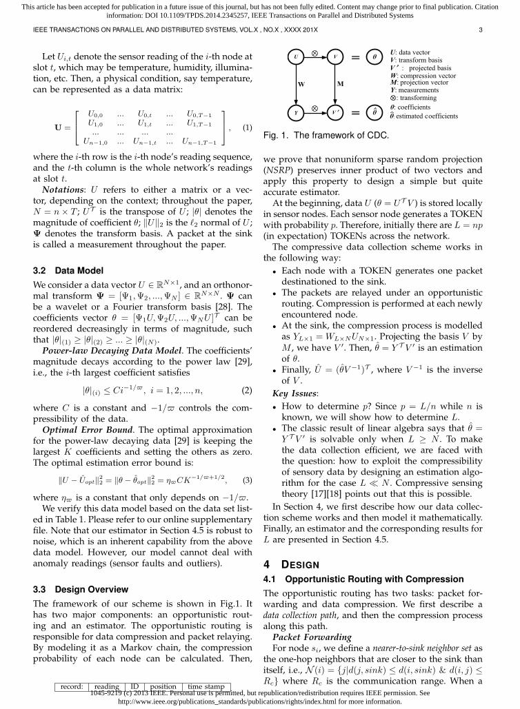
Data CompressionAs the packet travels towards the sink, the compres-

sion scheme adds or substracts the sensory reading ofa newly encountered node, as shown in Fig.2(a). Theformat of the data packet is:

Packet: value ID list coefficient list time stamp list

Let ui (i = 0, 1, ..., ρl − 1) be the reading of thei-th node along path Pl. The data compression isperformed as following:Step 1: A node with the l-th TOKEN becomes node p0of Pl. It generates a packet containing data y0 = ±u0,then transmits the packet to one of its nearer-to-sinkneighbors according to the opportunistic routing.Step 2: The packet arrives at sensor si, who adds orsubstracts its own sensor ready with probability 1/2as:

yi = yi−1 + riui, (4)

Sensor ID, the coefficient ri and the current time slotis added to the packet’s header. Then si transmits itto one of its neighbors closer to the sink according tothe opportunistic routing.Step 3: The encoding process continues along path Pl

until the packet reaches the sink.From the proof of Lemma. 1 (in Section 4.2), we

know that the random coefficients ri can be realvalues in [−1, 1] or chosen from −1,+1. We usethe set −1,+1 because the nodes will only need toperform addition or substraction operations.

In the end of the data compression process, L = nppackets are collected by the sink. Next, we considerthe sink’s strategy to estimate the sensor readings.

4.2 Problem Formulation for EstimationTraditional Compressive Sensing Approach. In tradi-tional compressive sensing approach [11][23][24], thesink establishes the following equation:

YL×1 = AL×NUN×1, (5)

Fig. 2. (a) Along Pl, the packet adds or subtractsthe sensor reading of a newly encountered node. (b)The left process is modelled as: a sampling processf randomly selects a subset of sensor readings, anda compression process sums them up with randomcoefficients chosen from the set −1,+1 to get onemeasurement.

where A is an matrix with elements corresponding tori in Eqn.(4). The sink can extract A from the collectedpackets’ headers.

Assuming that data U is sparse. To be exact, thereexists a transform basis VN×N under which UN×1 canbe represented using K ≪ n nonzero coefficients,i.e., θ = UT V with ∥θ∥0 = K. Compressive sensingtheory (CS) [17][18] claims that, with probability atleast 1 − n−γ (γ is set to be large), U can be recon-structed exactly as the solution to the following ℓ1-minimization problem, i.e., U = (θV −1)T where

θ = minθ

N∑i=1

|θi|, s.t. YL×1 = AL×NUN×1

L = O(Kµ2(A,V )logN/K), µ(A,V ) = max

1≤i,j≤N|AT

i Vj |.(6)

Existing approaches suggest to densely compressWSNs’ data to get random measurements as in[11][19]. Compressive sensing allows one to use con-vex optimization to estimate sensory readings underthe condition of the RIP property [17][18], i.e., todecouple the matrix A and the basis V to have smallvalue of µ. However, the RIP property does nothold for opportunistic routings, which postpones itsutilization [24][25].

Problem Formulation. We take another approachby regarding the compression process as nonuniformsparse random projections (shown in Fig.2(b)), modeledas two mutually independent processes nonuniformsampling process f(·) and linear encoding A as:

f(Uj) =

Uj , prob. πj

0, prob. 1− πj, Aij =

1, prob. 1

2

−1, prob. 12

, (7)

where πj = 0, j ∈ 1, 2, ..., N corresponds to the chanceof Uj being compressed in the collected packets. Thus,we model the compression scheme as:

YL×1 = AL×Nf(UN×1). (8)

Our problem becomes:

θ = minθ

∥U − U∥22,

s.t. YL×1 = AL×Nf(UN×1),(9)




where U = (θV −1)T .The opportunistic routing provides load balancing

in the cost of nonuniform compression probabilityof each node [24][25]. This leads to the failure ofthe traditional compressive sensing approach. In thefollowing section, we provide a method to calculatethe compression probability for each node. Then inSection 4.5, we introduce a new estimation algorithmby using the information of compression probabilityof each node.

4.3 Compression Probability EstimationModeling the Opportunistic Routing as a MarkovChain. The packet forwarding process can be modeledas a Markov Chain: the states are the nodes, andthe forwarding probability constitutes the transitionprobability matrix (each entry specifies the probabilitythat a packet is transmitted from one node to one ofits nearer-to-sink neighbors).

First, we estimate the transition matrix P basedon the “incomplete observation” version of maximumlikelihood estimation. Once the transition matrix P isknown, the compression probability distribution π canbe derived.

The Incomplete Observation Problem. For each pairof nodes, assume that there is a transition link with twostates: ON and OFF. If we have complete observationsof all links’ states in each time slot, then the estimationof the transition matrix is to maximize the log-likelihoodof the posterior probability, i.e., log P ((P1, P2, ...PL)|P )with (P1, P2, ...PL) denotes the data collection pathsof the L collected packets. Maximum likelihood esti-mation (MLE) is the most used routine to solve thisproblem [33].

However, the observation of a transition link’s stateis to try a “packet-transmitting test”, which is contra-dict to our goal as the data collection aims to minimizethe number of packets transmitted. Therefore, with“incomplete” or under-sampled observations, the tra-ditional MLE scheme can not be used here.

MLE with Incomplete Observation. Here, we adoptan “incomplete observation” version of MLE [34].Let Oijt denote the number of observed transitionfrom node si to node sj occurring over t time slotsand (P t)ij the ij-th element of the matrix P t (theprobability of a packet in node si arrives at node sjafter t time slots), this new MLE is defined as:

P = maxP

log P ((P1, P2, ...PL)|P )

= maxP

∑i

∑j

∑t

Oijtlog(Pt)ij .

(10)

It is proved in [34] that the expectation maximizationalgorithm converges to the global maximum. Whichmeans that with high probability, the above maximiz-er can produce an accurate transition matrix.

Estimation of the Compression Probability π.The compression probability closely relates with the

Markov chain-like occurrence, except that we shouldonly count one time if the packet stays at a nodewaiting for transmission. The estimation algorithm isdescribed as following:Step 1: Initially, π0 = L/n, ..., L/n.Step 2: Get P by setting P ’s diagonal elements to 0.Step 3: Calculate the nodes’s occurrence frequency indata collection paths during T time slots:

Oi(T ) =

T−1∑i=0

π0Pi. (11)

Step 4: Average the occurrence frequency by∑

π0, weget the probability distribution

πi =Oi(T )∑

π0=

∑T−1i=0 π0P

i∑π0

, (12)

where the sum and division are element-wise opera-tions on row vectors.

4.4 Nonuniform Sparse Random ProjectionEqn.(8) equals to the following linear equations:

YL×1 = WL×NUN×1, (13)

Wij =

+1, prob. 12πj

0, prob. 1− πj

−1, prob. 12πj

. (14)

Sparse and nonuniform raise from the fact that theopportunistic routing will neither pass all sensor n-odes nor pass them with equal probability, which isthe case for most existing routings. Sparse allows thecollected packets to compress sensor readings from arandom selected subset, while traditional compressivesensing approaches require to compress all sensoryreadings together, or the subset are randomly selectedwith equal probability [11][19].

Correspondingly, we construct a projection matrixM ∈ RL×N (where L ≪ N ) containing entries

Mij =1

πj

+1, if Wij = +1

0, if Wij = 0

−1, if Wij = −1

. (15)

The entries within each row are mutual-independent,while the entries across different rows are fully inde-pendent. In expectation, each row contains

∑nj=1 πj

nonzero elements, i.e., there are on average∑n

j=1 πj

sensor readings encoded in one collected packet.Next, we prove in Lemma 1 that with high proba-

bility, nonuniform sparse random projections preserveinner products with predictable error. Therefore, usingonly their random projections, we are able to estimatethe inner product of two vectors. The detailed proofis in the next section.

Lemma 1 For any vectors U, V ∈ RN×1, and W,M ∈RL×N in Eqn.(14)(15). The random projections Y =




1√LWU, V ′ = 1√

LMV , with the expectation and variance

satisfying:E[Y T V ′] = UT V, (16)

V ar(Y T V ′) ≤ 1

L((UT V )2 + ξ∥U∥22∥V ∥22

+ (κ− 2− ξ)

N∑j=1

U2j V

2j ),

(17)

where ξ = max( πl

πm)(l,m ∈ 1, 2, ...n), κ = 1

min(π)

denote the degree of nonuniform and the expected timesto sample the “rarest” node, respectively.

4.5 NSRP-based EstimatorThe intuition for our estimator design is that nonuni-form sparse random projections preserve inner productswithin a small error. Hence we can use random linearmeasurements Y = WU of the original data, and ran-dom linear projections V ′ = MV of the orthonormalbasis, to estimate the coefficients vector θ, as in thefollowing way:Step 1: Extract packets’ headers at the sink, get WL×N

,YL×1, and the projection matrix M .Step 2: Set L1 = C1

1+ξ+κH2

ϵ2 and L2 = C2(1 + γ) logNsuch that L = L1L2.Step 3: Partition YL×1 into L2 column vectorsY1, Y2, ..., YL2 with each of size L1 × 1, partition Minto M1,M2, ...,ML2 with each of size L1 ×N , thenproject the basis V to get V ′

1 = 1√L1

M1V, · · · , V ′L2

=1√L1

ML2V .Step 4: Compute ζl = Y T

l V ′l , l = 1, 2, · · · , L2. Set

each element of θ as the median value of each columnvector ζ1, ..., ζL2 .Step 5: Keep the K largest coefficient in θ and set theremaining to zero.Step 6: Return U = (θV −1)T .

The following two theorems hold for the above esti-mator. Please refer to the next section for the detailedproof for Theorem 1. Since the proof of Theorem 2 issimilar to that in [26], for completeness, we include itin the supplementary file.

Theorem 1 For data vector U ∈ RN×1 satisfying

∥U∞∥∥U∥2

≤ H. (18)

Let V = V1, ..., VN be the transform basis with eachvector RN×1, W,M ∈ RL×N as in Eqn.(14)(15) with thecompression probability π, L =

O( 1+γϵ2

(ξ + κH2)logn), if (ξ + κH2) > Ω(1)

O( 1+γϵ2

logn), if (ξ + κH2) ≤ O(1)(19)

Then, with probability at least 1 − N−γ , the randomprojections Y = 1√

LWU and V ′ = 1√

LMVi can produce

an estimate θi for UT Vi (Step 4 in the above estimator),satisfying

|θi − UT Vi| ≤ ϵ∥U∥22∥Vi∥22 (20)

for all i = 1, 2, ..., N .

Theorem 2 Suppose data U ∈ RN×1 satisfies condition(18), W,M ∈ RL×N in Eqn.(14)(15) with probabilitydistribution π, and L =O( 1+γ

ϵ2η2 (ξ + κH2)K2logn), if(ξ + κH2) ≥ Ω(1)

O( 1+γϵ2η2K

2logn), if(ξ + κH2) ≤ O(1).(21)

Let Y = 1√LWU , consider an orthonormal transform Ψ ∈

RL×N and the corresponding transform coefficients θ =ΨU . If the K largest transform coefficients in magnitudegive an approximation with error ∥U − Uopt∥ ≤ η∥U∥22,then given only Y,W,M and Ψ, the above NSRP-basedestimator produces an estimate U with error

∥U − U∥ ≤ (1 + ϵ)η∥U∥22 (22)

with probability at lest 1−N−γ .

For the above estimator, Theorem 1 states that withhigh probability, the nonuniform sparse random pro-jections of data vector and any projected basis vectorcan produce estimates of their inner products withina small error. Thus Theorem 1 guarantees small es-timation error for each coefficient. Theorem. 2 showsthat with high probability, nonuniform sparse randomprojections can approximate compressible data witherror being comparable to the optimal error bound(by setting ϵ to be small, i.e, ϵ = o(1).). Thus, withhigh probability, the above estimator produces anestimation of the original data within small error.

Note that compared with uniform sampling [26],nonunifrom sampling requires bigger L. For the extra(ξ+ κH2) component, ξ can be regarded an indicatorof the degree of nonuniform, and κ is a factor toguarantee successful decoding for the “rarest” node.

5 PROOFS

5.1 Lemma 1

Proof: The pair of nonuniform sparse randomprojections W,M ∈ RL×n satisfies:

E[Wij ] = 0, E[Mij ] = 0;E[WijMij ] = 1,

E[WilMim] = E[Wil]E[Mim] = 0 if l = m,

E[WilMilWimMim] = E[WilMil]E[WimMim] = 1 if l = m,

E[W 2ij ] = πj , E[M2

ij ] =1

πj, E[W 2

ijM2ij ] =

1

πj,

E[W 2ilM

2im] = E[W 2

il]E[M2im] =

πl

πmif l = m.

The above results will be used in the following processwithout explicit mention.

Define the random variables

ωi =

(n∑

j=1

ujWij

)(n∑

j=1

vjMij

)

ζ = αTβ =1

L

L∑i=1

ωi




so that ω1, ω2, ..., ωM are independent.

E(ωi) = E

n∑j=1

ujvjWijMij +∑l=m

ulvmWilMim

=

n∑j=1

ujvjE[WijMij ] +∑l=m

ulvmE[WilMim]

= uTv

E[ζ] = uTv

Similarly, we can compute the second moments andvariance as following:

E[ω2i ] = E

( n∑j=1

ujvjWijMij

)2

+

∑l =m

ulvmWilMim

2

+2

(n∑

j=1

ujvjWijMij

)∑l=m

ulvmWilMim

=

n∑j=1

u2jv

2jE[W 2

ijM2ij ] + 2

∑l<m

ulvlumvmE[WilMilWimMim]

+∑l=m

u2l v

2mE[W 2

ilM2im] + 2

∑l<m

ulvmumvlE[WilMilWimMim]

=

n∑j=1

u2jv

2j1

πj+ 2

∑l=m

ulvlumvm +∑l=m

u2l v

2m

πl

πm

(Let ξ = max(πl

πm), κ =

1

min(π))

≤ 2

n∑j=1

u2jv

2j + 2

∑l=m

ulvlumvm

+ ξ

n∑j=1

ujvj +∑l=m

u2l v

2m

+ (κ− 2− ξ)

n∑j=1

ujvj

= 2(u′v)2 + ξ∥u∥22∥v∥22 + (κ− 2− ξ)n∑

j=1

u2jv

2j

V ar(ωi) = E[ω2i ]− E[ωi]

2

≤ (u′v)2 + ξ∥u∥22∥v∥22 + (κ− 2− ξ)n∑

j=1

u2jv

2j

V ar(ζ) =1

L2

L∑i=1

V ar(ωi)

≤ 1

L

((u′v)2 + ξ∥u∥22∥v∥22 + (κ− 2− ξ)

n∑j=1

u2jv

2j

)

5.2 Theorem 1

Proof: Fix any two vectors u, v ∈ Rn, with∥u∥∞/∥u∥2 ≤ H . Set L = L1L2, with L1, L2 are posi-tive integers. Partition the L×n matrix W and M intoL2 matrices W1,W2, ...,WL2 and M1,M2, ...,ML2,each of size L1 × n. The corresponding random pro-jections are α1 = 1√

L1W1u, ..., αL2 = 1√

L1WL2u, and

β1 = 1√L1

W1v, ..., βL2 = 1√L1

WL2v.

Define the independent random variables ζl =α′lβl, l = 1, 2, ..., L2. Applying Lemma 1 to each ζl,

we derive that E[ζl] = u′v and

V ar(ζ) ≤ 1

L1((u′v)2+ ξ∥u∥22∥v∥22+(κ−2− ξ)

n∑j=1

u2jv

2j )

By the Chebyshev inequality and

P (|ζl − u′v| ≥ ϵ∥u∥2∥v∥2) ≤V ar(ζl)

ϵ2∥u∥22∥v∥22

≤ 1

ϵ2L1

((u′v)2

∥u∥22∥v∥22+

ξ∥u∥22∥v∥22∥u∥22∥v∥22

+ (κ− 2− ξ)

∑nj=1 u

2jv

2j

∥u∥22∥v∥22

)(By the Cauchy − Schwarz inequality and Eqn.(18))

≤ 1

ϵ2L1

(1 + ξ + κ

H2∥u∥22∑n

j=1 v2j

∥u∥22∥v∥22

)≤ 1

ϵ2L1

(1 + ξ + κH2) , p

Thus, we can obtain a constant probability p by settingL1 = O( 1+ξ+κH2

ϵ2 ).We define the estimate a as the median of the inde-

pendent random variables ζ1, ..., ζL2 , each of whichlies outside of the tolerable approximation intervalwith probability p. Formally, let Il be the indicator ran-dom variable of the event that |ζl−u′v| ≥ ϵ∥u∥2∥v∥2,which occurs with probability p.

Let I =∑

l=1 L2Il be the number of ζl’s that lieoutside of the tolerable interval, where E[I] = L2p.When the event that at least half of the ζl’s are outsidethe tolerable interval occurs with arbitrarily smallprobability, then the median a is within the tolerableinterval. So, if we set p < 1/2, say p = 1/4, and applythe Chernoff bound, we get:

P

(I > (1 + c)

L2

4

)< e−c2L2/12

where 0 < c < 1 is some constant.Thus, for u and vi ∈ v1, ..., vn ⊂ Rn, and the

corresponding random projections α and β producean estimate a for u′v that lies outside the tolera-ble approximation interval with probability at moste−c2L2/12. For the n estimates ai, i = 1, 2, ...n, theprobability that at least one lies outside the tolerableinterval is upper bounded by Pe ≤ ne−c2L2/12.

Setting L1 = O( 1+ξ+κH2

ϵ2 ) obtains p = 1/4, andsetting L2 = O((1 + γ)logn) obtains Pe ≤ n−γ forsome constant γ > 0. Therefore, with L = L1L2 =O( 1+γ

ϵ2 (1 + ξ + κH2)logn), the nonuniform randomprojection pair W,M can produce inner products ofvectors with probability at least 1 − n−γ . If (ξ +κH2) > Ω(1), then L = O( 1+γ

ϵ2 (1 + ξ + κH2)logn). If(ξ + κH2) ≤ O(1), then L = O( 1+γ

ϵ2 logn).

6 EVALUATION6.1 Simulation SettingsGround Truth. We use data sets collected from theGreenOrbs [35], IntelLab [36] and NBDC-CTD [37]




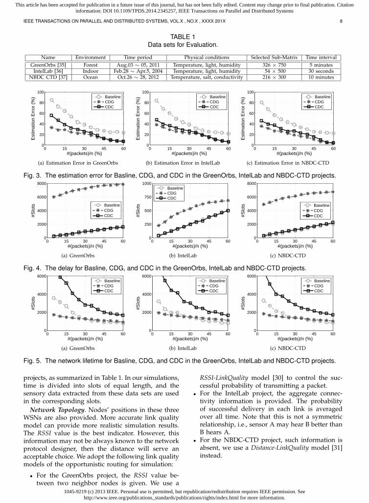
TABLE 1Data sets for Evaluation.

Name Environment Time period Physical conditions Selected Sub-Matrix Time intervalGreenOrbs [35] Forest Aug.03 ∼ 05, 2011 Temperature, light, humidity 326 × 750 5 minutes

IntelLab [36] Indoor Feb.28 ∼ Apr.5, 2004 Temperature, light, humidity 54 × 500 30 secondsNBDC CTD [37] Ocean Oct.26 ∼ 28, 2012 Temperature, salt, conductivity 216 × 300 10 minutes

0 15 30 45 600

20

40

60

80

100

#(packets)/n (%)

Est

imat

ion

Err

or (

%)

BaselineCDGCDC

(a) Estimation Error in GreenOrbs

0 15 30 45 600

20

40

60

80

100

#(packets)/n (%)

Est

imat

ion

Err

or (

%)

BaselineCDGCDC

(b) Estimation Error in IntelLab

0 15 30 45 600

20

40

60

80

100

#(packets)/n (%)

Est

imat

ion

Err

or (

%)

BaselineCDGCDC

(c) Estimation Error in NBDC-CTD

Fig. 3. The estimation error for Basline, CDG, and CDC in the GreenOrbs, IntelLab and NBDC-CTD projects.

0 15 30 45 600

2000

4000

6000

8000

#(packets)/n (%)

#Slo

ts

BaselineCDGCDC

(a) GreenOrbs

0 15 30 45 600

250

500

750

1000

#(packets)/n (%)

#Slo

ts

BaselineCDGCDC

(b) IntelLab

0 15 30 45 600

2000

4000

6000

8000

#(packets)/n (%)#S

lots

BaselineCDGCDC

(c) NBDC-CTD

Fig. 4. The delay for Basline, CDG, and CDC in the GreenOrbs, IntelLab and NBDC-CTD projects.

0 15 30 45 600

2000

4000

6000

#(packets)/n (%)

#Slo

ts

BaselineCDGCDC

(a) GreenOrbs

0 15 30 45 600

2000

4000

6000

#(packets)/n (%)

#Slo

ts

BaselineCDGCDC

(b) IntelLab

0 15 30 45 600

2000

4000

6000

#(packets)/n (%)

#Slo

ts

BaselineCDGCDC

(c) NBDC-CTD

Fig. 5. The network lifetime for Basline, CDG, and CDC in the GreenOrbs, IntelLab and NBDC-CTD projects.

projects, as summarized in Table 1. In our simulations,time is divided into slots of equal length, and thesensory data extracted from these data sets are usedin the corresponding slots.

Network Topology. Nodes’ positions in these threeWSNs are also provided. More accurate link qualitymodel can provide more realistic simulation results.The RSSI value is the best indicator. However, thisinformation may not be always known to the networkprotocol designer, then the distance will serve anacceptable choice. We adopt the following link qualitymodels of the opportunistic routing for simulation:

• For the GreenOrbs project, the RSSI value be-tween two neighbor nodes is given. We use a

RSSI-LinkQuality model [30] to control the suc-cessful probability of transmitting a packet.

• For the IntelLab project, the aggregate connec-tivity information is provided. The probabilityof successful delivery in each link is averagedover all time. Note that this is not a symmetricrelationship, i.e., sensor A may hear B better thanB hears A.

• For the NBDC-CTD project, such information isabsent, we use a Distance-LinkQuality model [31]instead.




6.2 Compared AlgorithmsBaseline. Packets are transmitted back to the sinkalong the shortest path. Then the sink applies the k-Nearest Neighbors (KNN) [38] method to estimate thereadings, i.e., by averaging the k-nearest neighbors’values. Since both the routing and estimation are themost basic ones, therefore we use it as the baselinealgorithm.

CDG (MobiCom’09). The CDG scheme compressesall sensor readings together in each collected packet.It uses the following tree-based routing: a node waitsfor all its children’s packets, performs random linearcompression, and then sends the packet to its parentnode. The estimation uses the convex optimizationmethod of traditional compressive sensing theory. Itis a bit different from [11] since the link quality isnot perfectly reliable as we allow the transmission tofail through a controlled probability and introduce theretransmission mechanism.

6.3 MetricsBased on the network topology and sensory datasets of these three wireless sensor networks, we runthe above three schemes to collect sensor readingsback to the sink. For the baseline algorithm and theCDC scheme, we vary the probability p of generatingTOKENs to get different number of random measure-ments. For equality, the CDG scheme will collect ac-cordingly the same number of random measurements.

Estimation ErrorEach algorithm estimates a U for the original data

U . The estimation error is defined as:

E =∥U − U∥2

∥U∥2. (23)

DelayThe data collection delay is defined as the time

when the last packet arrives at the sink, which ismeasured in terms of the number of slots.

Network LifetimeThe energy consumption is set according to the en-

ergy consumption model [39]. At the beginning, eachnode have initial energy of 1, 000, 000 units which cansupport the sensor node to run about a month. Thenetwork lifetime is defined as the time when the firstnode runs out of energy, which is also measured interms of the number of slots.

6.4 ResultsFrom Fig. 3(a)(b)(c), CDG and CDC perform muchbetter than the baseline algorithm and can reachestimation errors as low as 5%. This is because theyboth exploit the compressibility nature of the sensorreadings and use random compression techniques.However, CDG behaves better in situations whereless number of packets are collected. Possibly, less

collected packets can lead to (1) stronger nonuniformnature of the compression probability of sensor nodes,or (2) less observations of the routing process, thenless accurate of probability estimation in Section 4.3.

From Fig. 4(a)(b)(c), it is quite unexpected that thedelay of the CDG scheme is several or even hundredsof times longer than the other two. The reason maybethat: CDG tries to encode every node’s packets, anda parent node has to wait for all its children’s packetsbefore transmitting the compressed packet to its ownparent node. Because the network size of the IntelLabproject is smaller, the delay performance is closer forthese three schemes. The baseline algorithm exhibitsa good, stable, and moderate growth in delay sinceit used the shortest path routing. The CDC’s routingstrategy is quite similar with the baseline scheme,therefore it experiences quite similar performance interms of delay.

From Fig. 5(a)(b)(c), we find that our scheme has thebest performance. For estimation error within 20%,CDC prolongs the network lifetime by 1.5× ∼ 2×.This is because that CDC requires fewer measure-ments, even fewer number of sensory readings ineach measurement, thus greatly reduces the energyconsumption.

7 CONCLUSION AND FUTURE WORK

We have proposed a novel compressive data collectionscheme for wireless sensor networks. This schemeleverages the fact that raw sensory data have strongspatiotemporal compressibility. Our scheme consistsof two parts: the opportunistic routing with compres-sion, and the nonuniform random projection based es-timation. The proposed scheme agrees with Braniuk’s[1] suggestion that sensory data acquisition should bemore efficient, and the new techniques that combinesensing and network communication together is apromising approach. We prove that this scheme canachieve optimal approximation error, and trace basedevaluations show that its error is comparable withthe existing method [11]. More important, our schemeexhibits good performance for energy-conservation.

In the future, we will apply this nonuniform ran-dom projection based estimator for adaptive datagathering [40] and the multiple attributes scenario[41].

ACKNOWLEDGMENT

This research was supported by NSFC undergrant No. 61303202, No. 61073158, No. 61100210,STCSM Project No. 12dz1507400, FQRNT grant131844, Singapore-MIT IDC IDD61000102a, SUTD-ZJU/RES/03/2011, and NRF2012EWT-EIRP002-045.Xiao-Yang Liu gratefully acknowledges financial sup-port from China Scholarship Council.




REFERENCES

[1] R.G. Baraniuk, “More is less: Signal processing and the datadeluge”, Science, Vol. 331, No. 6018, pp. 717-719, 2011.

[2] I.F. Akyildiz, W. Su, Y. Sankarasubramaniam, and E. Cayirci,“Wireless sensor networks: a survey”, Elsevier Computer Net-works, Vol. 38, No. 4, pp. 393-422, 2002.

[3] T. Bokareva, W. Hu, S. Kanhere, B. Ristic, N. Gordon, T. Bessell,M. Rutten, and S. Jha, “Wireless sensor networks for battlefieldsurveillance”, Proc. the land warfare conference, 2006.

[4] L. Kong, M. Zhao, X.-Y. Liu, J. Lu, Y. Liu, M.-Y. Wu, andW. Shu, “Surface coverage in sensor networks, IEEE Trans-actions on Parallel and Distributed Systems, Vol. 25, No. 1, pp.234-243, 2014.

[5] X.-Y. Liu, K.-L. Wu, Y. Zhu, L. Kong, and M.-Y. Wu, “Mobilityincreases the surface coverage of distributed sensor networks”,Elsevier Computer Networks, Vol. 57, No. 11, pp. 2348-2363, 2013.

[6] R. Szewczyk, A. Mainwaring, J. Polastre, J. Anderson, andD. Culler, “An analysis of a large scale habitat monitoringapplication”, ACM Sensys, pp. 214-226, 2004.

[7] S. Kim, S. Pakzad, D. Culler, J. Demmel, G. Fenves, S. Glaser,and M. Turon, “Health monitoring of civil infrastructuresusing wireless sensor networks”, ACM/IEEE IPSN, pp. 254-263, 2007.

[8] L. Selavo, A. Wood, Q. Cao, T. Sookoor, H. Liu, A. Srinivasan,Y. Wu, W. Kang, J. Stankovic, D. Young, and J. Porter, “Luster:wireless sensor network for environmental research”, ACMSensys, pp. 103-116, 2007.

[9] P. Gupta and P.R. Kumar, “The capacity of wireless networks”,IEEE Transactions on Information Theory, Vol. 46, No. 2, pp. 388-404, 2000.

[10] L. Fu, Y. Qin, X. Wang, and X. Liu, “Converge-cast withmimo”, IEEE INFOCOM, pp. 649-657, 2011.

[11] C. Luo, F. Wu, J. Sun, and C.W. Chen, “Compressive datagathering for large-scale wireless sensor networks”, ACMMobiCom, pp. 145-156, 2009.

[12] L. Kong, M. Xia, X.-Y. Liu, M.-Y. Wu, and X. Liu, “Data lossand reconstruction in sensor networks”, IEEE INFOCOM, pp.1654-1662, 2013.

[13] F. Fazel, M. Fazel, and M. Stojanovic, “Random access com-pressed sensing for energy-efficient underwater sensor net-works”, IEEE Journal Selected Areas in Communications (JSAC),29(8), pp. 1660-1670, 2011.

[14] E. Fasolo, M. Rossi, J. Widmer, and M. Zorzi, “In-network ag-gregation techniques for wireless sensor networks: a survey”,IEEE Wireless Communications, Vo. 14, No. 2, pp. 70-87, 2007.

[15] R. Cristescu, B. Beferull-Lozano, and M. Vetterli, “On networkcorrelated data gathering”, IEEE INFOCOM, pp. 2571-2582,2004.

[16] J. Haupt, W.U. Bajwa, M. Rabbat, and R. Nowak, “Compressedsensing for networked data”, IEEE Signal Processing Magazine,Vol. 25, No. 2, pp. 92-101, 2008.

[17] E.J. Candes, J. Romberg, and T. Tao, “Robust uncertaintyprinciples: Exact signal reconstruction from highly incompletefrequency information”, IEEE Transactions on Information The-ory, 52(2), pp. 489-509, 2006.

[18] E.J. Candes and T. Tao, “Near-optimal signal recovery fromrandom projections: Universal encoding strategies?” IEEETransactions on Information Theory, Vol. 52, No. 12, pp. 5406-5425, 2006.

[19] H. Zheng, F. Yang, X. Tian, X. Gan, X. Wang, and S. Xiao,“Data gathering with compressive sensing in wireless sensornetworks: a random walk rased approach”, IEEE Transactionson Parallel and Distributed Systems, 2014.

[20] G. Anastasi, M. Conti, M. Di Francesco, and A. Passarella,“Energy conservation in wireless sensor networks: A survey”,Ad Hoc Networks, Vol. 7. No. 3, pp. 537-568, 2009.

[21] R. Cristescu, B. Beferull-Lozano, and M. Vetterli, “Networkcorrelated data gathering with explicit communication: NP-completeness and algorithms”, IEEE/ACM Transactions on Net-working (ToN), Vol. 14, No. 1, pp. 41-54, 2006.

[22] X. Liu, J. Luo, A.V. Vasilakos, “Compressed data aggregationfor energy efficient wireless sensor networks”, IEEE SECON,pp. 46-54, 2011.

[23] L. Guo, R. Beyah, and Y. Li, “Smite: a stochastic compressivedata collection protocol for mobile wireless sensor networks”,IEEE INFOCOM, pp. 1611-1619, 2011.

[24] W. Xu, E. Mallada, and A. Tang, “Compressive sensing overgraphs”, IEEE INFOCOM, pp. 2087-2095, 2011.

[25] G. Quer, R. Masiero, D. Munaretto, M. Rossi, J. Widmer,and M. Zorzi, “On the interplay between routing and signalrepresentation for compressive sensing in wireless sensor net-works”, IEEE Information Theory and Applications Workshop, pp.206-215, 2009.

[26] W. Wang, M. Garofalakis, and KW Ramchandran, “Distributedsparse random projections for refinable approximation”, IEEEIPSN, pp. 331-339, 2007.

[27] D. Baron, S. Sarvotham, R.G. Baraniuk, “Bayesian compressivesensing via belief propagation”, IEEE Transactions on SignalProcessing, Vol. 58, No. 1, pp. 269-280, 2010.

[28] J. Haupt, W.U. Bajwa, M. Rabbat, R. Nowak, “Compressedsensing for networked data”, IEEE Signal Processing Magazine,Vol. 25, No. 2, pp. 92-101, 2008.

[29] A. Cohen, W. Dahmen, and R. DeVore, “Compressed sensingand best k-term approximation”, J. Amer. Math. Soc, 22(1), pp.211-231, 2009.

[30] M.H. Lu, P. Steenkiste, and T. Chen, “Design, implementationand evaluation of an efficient opportunistic retransmissionprotocol”, ACM MobiCom, pp. 73-84, 2009.

[31] S. Biswas and R. Morris, “Opportunistic routing in multi-hopwireless networks”, ACM SIGCOMM Computer CommunicationReview, Vol. 34, No. 1, pp. 69-74, 2004.

[32] S. Chachulski, M. Jennings, S. Katti, and D. Katabi, “Tradingstructure for randomness in wireless opportunistic routing”,ACM SIGCOMM, Vol. 37, No. 4, pp. 169-180, 2007.

[33] S. Johansen and K. Juselius, “Maximum likelihood estimationand inference on cointegrationłwith applications to the de-mand for money”, Oxford Bulletin of Economics and statistics,52(2), pp. 169-210, 1990.

[34] C. Sherlaw-Johnson, S. Gallivan, and J. Burridge, “Estimatinga markov transition matrix from observational data”, Journalof the Operational Research Society, pp. 405-410, 1995.

[35] Y. Liu, Y. He, M. Li, J. Wang, K. Liu, L. Mo, W. Dong, Z. Yang,M. Xi, J. Zhao, and X.-Y. Li, “Does wireless sensor networkscale? a measurement study on greenorbs”, IEEE INFOCOM,pp. 873-881, 2011.

[36] IntelLab data.http://www.select.cs.cmu.edu/data/labapp3/index.html.

[37] NBDC-CTD data.http://tao.noaa.gov/refreshed/ctd delivery.php.

[38] T. Cover and P. Hart, “Nearest neighbor pattern classification”,IEEE Transactions on Information Theory, Vol. 13, No. 1, pp. 21-27, 1967.

[39] X. Jiang. M.V. Ly, J. Taneja, P. Dutta, and D. Culler, “Experi-ences with a high-fidelity wireless building energy auditingnetwork”, ACM Sensys, pp. 113-126, 2009.

[40] L. Kong, X.-Y. Liu, M. Tao, M.-Y. Wu, Y. Gu, L. Cheng, andJ. Niu, “Resource-efficient data gathering in sensor networksfor environment reconstruction, to appear in The ComputerJournal, 2014.

[41] G. Chen, X.-Y. Liu, L. Kong, J.-L. Lu, and M.-Y. Wu, “Multi-attribute compressive data gathering, IEEE WCNC, 2014.




Xiao-Yang Liu received his B.Eng. degree incomputer science from Huazhong Universityof Science and Technology, China, in 2010.He is currently working toward the PhD de-gree in the Department of Computer Scienceand Engineer in Shanghai Jiao Tong Univer-sity. His research interests include wirelesscommunication, sensor networks, and dis-tributed systems.

Yanmin Zhu (M’02) received the PhD degreein computer science from Hong Kong Univer-sity of Science and Technology in 2007. Heis an associate professor in the Departmen-t of Computer Science and Engineering atShanghai Jiao Tong University. His researchinterests include vehicular networks, sensornetworks, mobile computing. Prior to joiningShanghai Jiao Tong University, he was aresearch associate with the Department ofComputing at the Imperial College London.

He is a member of the IEEE and IEEE Communication Society.

Linghe Kong (S’09-M’13) is currently aresearch assistant professor in ShanghaiJiao Tong University and a postdoctoral re-searcher in Singapore University of Tech-nology and Design. He received his PhDdegree in Computer Science with ShanghaiJiao Tong University 2012, Dipl. Ing. degreein Telecommunication with TELECOM Sud-Paris 2007, B. E. degree in Automation withXidian University 2005. His research inter-ests include wireless sensor networks and

mobile computing.

Cong Liu is an assistant professor in theDepartment of Computer Science at the U-niversity of Texas at Dallas. He received hisPh.D. degree in Computer Science from theUniversity of North Carolina at Chape Hillin July 2013. His research interests includereal-time and embedded systems, operat-ing systems, cloud computing, and wirelesssensor networks. He has published over 30papers in premier conferences and journalssuch as RTSS, PACT, ECRTS, and JPDC. He

received the Best Student Paper Award at the 30th IEEE Real-TimeSystems Symposium, the premier real-time and embedded systemsconference. He also received the best papers award at the 17thRTCSA and the UNC’s dissertation fellowship.

Yu (Jason) Gu is currently an assistantprofessor in the Pillar of Information Sys-tem Technology and Design at the Singa-pore University of Technology and Design.He received the Ph.D. degree from the U-niversity of Minnesota, Twin Cities in 2010.His research includes Networked Embed-ded Systems, Wireless Sensor Networks,Cyber-Physical Systems, Wireless Network-ing, Real-time and Embedded Systems, Dis-tributed Systems, Vehicular Ad-Hoc Net-

works and Stream Computing Systems.

Athanasios V. Vasilakos (M’00-SM’11) iscurrently a Professor with the University ofWestern Macedonia, Greece. He served oris serving as an editor for many techni-cal journals, such as the IEEE Transac-tions on network and service managemen-t, IEEE Transactions on Cloud Computing,IEEE Transactions on information forensicsand security, IEEE Transactions on cybernet-ics, IEEE Transactions on Nanobioscience,IEEE Transactions on information technology

in biomedicine, ACM Transactions on autonomous and adaptivesystems, the IEEE Journal on Selected Areas in Communications.He is also General Chair of the European Alliances for Innovation(www.eai.eu).

Min-You Wu (S’84-M’85-SM’96) received theM.S. degree from the Graduate School ofAcademia Sinica, Beijing, China, in 1981 andthe Ph.D. degree from Santa Clara Universi-ty, Santa Clara, CA in 1984. He is a profes-sor in the Department of Computer Scienceand Engineering at Shanghai Jiao Tong U-niversity and a research professor with theUniversity of New Mexico. He serves as theChief Scientist at Grid Center of ShanghaiJiao Tong University. His research interests

include grid computing, wireless networks, sensor networks, multi-media networking, parallel and distributed systems, and compilersfor parallel computers.

ieee transactions on parallel and distributed...

Documents