ieee transactions on pattern analysis and …ravir/papers/refshare/reflectancesharing...efficient...

Reflectance Sharing: Predicting Appearancefrom a Sparse Set of Images of a Known Shape

Todd Zickler, Member, IEEE, Ravi Ramamoorthi, Sebastian Enrique, and Peter N. Belhumeur

Abstract—Three-dimensional appearance models consisting of spatially varying reflectance functions defined on a known shape can beused in analysis-by-synthesis approaches to a number of visual tasks. The construction of these models requires the measurement ofreflectance, and the problem of recovering spatially varying reflectance from images of known shape has drawn considerable interest. Todate, existing methods rely on either: 1) low-dimensional (e.g., parametric) reflectance models, or 2) large data sets involving thousands ofimages (or more) per object. Appearance models based on the former have limited accuracy and generality since they require theselection of a specific reflectance model a priori, and while approaches based on the latter may be suitable for certain applications, they aregenerally too costly and cumbersome to be used for image analysis. We present an alternative approach that seeks to combine thebenefits of existing methods by enabling the estimation of a nonparametric spatially varying reflectance function from a small number ofimages. We frame the problem as scattered-data interpolation in a mixed spatial and angular domain, and we present a theorydemonstrating that the angular accuracy of a recovered reflectance function can be increased in exchange for a decrease in its spatialresolution. We also present a practical solution to this interpolation problem using a new representation of reflectance based on radialbasis functions. This representation is evaluated experimentally by testing its ability to predict appearance under novel view and lightingconditions. Our results suggest that since reflectance typically varies slowly from point to point over much of an object’s surface, we canoften obtain a nonparametric reflectance function from a sparse set of images. In fact, in some cases, we can obtain reasonable results inthe limiting case of only a single input image.

Index Terms—Reflectance, BRDF, image synthesis, image-based rendering, radial basis functions.

�

1 INTRODUCTION

THREE-DIMENSIONAL appearance models consisting of ex-plicit shape models and spatially varying reflectance

functions defined on these shapes are effective tools foranalysis-by-synthesis approaches to recognition, tracking,and other visual tasks. This approach to image analysisprovides the advantage of separating intrinsic objectproperties (i.e., shape and material properties) fromextrinsic scene properties, such as pose, illumination, andcamera parameters.

Constructing an appearance model of a given objectrequires two stages: recovery of both shape and reflectance.Yet, while great strides have been made at recovering objectshape (laser-scanners, structured-light systems, multiviewstereo, photometric stereo, Helmholtz stereo, etc.), lessprogress has been made at recovering reflectance properties.Recovering and efficiently representing reflectance is difficultbecause of its inherent high-dimensionality. At each surfacepoint, reflectance is described by a four-dimensional functionof the view and lighting directions termed the bidirectionalreflectance distribution function (BRDF) [1]. The BRDFgenerally changes spatially over an object’s surface, andrecovering this spatially varying BRDF (or 6D SBRDF)without further assumptions typically requires a set of images

large enough to densely sample high-frequency radiometricevents, such as sharp specular highlights, at each point on thesurface. This set consists of an exhaustive sampling of imagesof the object from all viewpoints and lighting directions,which can be tens of thousands of images or more.

For vision applications, recovering and representingspatial reflectance is often made tractable by approximat-ing it with an analytic BRDF model. This reduces spatialreflectance from a 4D function at each point to either ahandful of parameters (see [2], [3], [4] for recent examples),or in the Lambertian case, to a single parameter at eachpoint. The parametric approach is also common for image-based rendering applications in computer graphics [5], [6],[7]. From an acquisition stand-point, since they onlyrequire a few parameters at each point, these methodsare able to provide reflectance estimates from a smallnumber of input images. They require the selection of aspecific parametric BRDF model a priori, however, whichlimits their accuracy and generality. For example, theCook-Torrance model [8] represents some plastics andmetals quite well but is unable to capture retro-reflectioneffects observed in other materials [9], [10].

Another approach—one that avoids the restrictions ofparametric reflectance models—is purely data-driven andrelies on densely sampling the BRDF at each point. Thisapproach is more common in graphics applications, in whichhundreds [11], thousands [12], or tens of thousands [13] ofimages are used to capture the reflectance information for agiven object.1 While these data-driven appearance models areuseful for image-based rendering applications, they are toocumbersometobeusedfor imageanalysis,andthehighcostof

IEEE TRANSACTIONS ON PATTERN ANALYSIS AND MACHINE INTELLIGENCE, VOL. 28, NO. 8, AUGUST 2006 1

. T. Zickler is with the Division of Engineering and Applied Sciences,Harvard University, 33 Oxford St., Cambridge, MA 02138.E-mail: [email protected].

. R. Ramamoorthi, S. Enrique, and P.N. Belhumeur are with the ComputerScience Department, Columbia University, 500 W 120 St., New York, NY10027. E-mail: {ravir, senrique, belhumeur}@cs.columbia.edu.

Manuscript received 22 June 2005; revised 22 Nov. 2005; accepted 5 Dec.2005; published online 13 June 2006.Recommended for acceptance by S. Seitz.For information on obtaining reprints of this article, please send e-mail to:[email protected], and reference IEEECS Log Number TPAMI-0326-0605.

1. These methods actually capture only a subset of the reflectanceinformation since even these large numbers of images are insufficient todensely sample the complete 4D BRDF at each point.

0162-8828/06/$20.00 � 2006 IEEE Published by the IEEE Computer Society

acquisition means that they cannot be used, for example, forlarge-scale enrollment in face/object recognition databases.

In this paper, we present an alternative approach thatmoves toward the acquisition of nonparametric spatialreflectance from a small number of images. This approachseeks to combine the benefits of both parametric methods (i.e.,sparse images) and purely data-driven, nonparametricmethods (i.e., arbitrary reflectance functions). The centralidea is that SBRDF estimation can be framed as a scattered-data interpolation problem, with images providing dense2D slices of data embedded in the mixed spatial and angulardomain. This approach is very different from previousnonparametric techniques (e.g., [11], [12], [13]) that inter-polate reflectance only in the angular dimensions, estimatinga unique reflectance function at each point. Instead, wesimultaneously interpolate in both the spatial and angulardimensions. This enables a controlled exchange betweenspatial and angular information, effectively giving up some ofthe spatial resolution in order to fill the holes betweensparsely observed view and illumination conditions. Sincereflectance (especially the specular component) typicallyvaries slowly from point to point over much of an object’ssurface, this means that we can often obtain good results froma drastically reduced set of images.

We first present a theoretical analysis showing how theangular accuracy of the SBRDF can be increased in exchangefor a reduction in its spatial resolution. We then provide apractical solution to the SBRDF estimation problem byintroducing: 1) a new parameterization of the BRDF domain,and 2) a nonparametric representation of reflectance based onradial basis functions (RBFs). In addition to providing anefficient solution to our SBRDF interpolation problem, thisrepresentation has two benefits. First, the resulting appear-ance model degrades gracefully (in the sense of providingvisually pleasing results) as the number of input imagesdecreases. It can even be applied in the limiting case of a singleinput image. Second, it is relatively dimension-independentand can therefore be adapted to represent homogeneousBRDF data, making it useful for image-based BRDF acquisi-tion systems [10], [14], [15].

2 MAIN IDEAS AND RELATED WORK

The proposed method for SBRDF estimation builds on threeprincipal observations.

Smooth Spatial Variation. Most existing methods recovera unique BRDF at each point and thereby provide an SBRDFwith very high spatial resolution. Many parametric methodshave demonstrated, however, that the number of inputimages can be reduced if one is willing to accept a decrease inspatial resolution. This has been exploited, for example, by Yuet al. [7], Georghiades [2], and Hara and Nishino [4], whoassume that specular BRDF parameters are constant across asurface.2 (The morphable model introduced by Blanz andVetter [3] relies on this assumption as well.) Similarly, Satoet al. [6] estimate the specular parameters at only a small set ofpoints, later interpolating these parameters across the sur-face. Lensch et al. [16] present a novel technique in whichreflectance samples at clusters of surface points are used toestimate a basis of (1-lobe) Lafortune models. The reflectance

at each point is then uniquely expressed as a linearcombination of these basis BRDFs.

Similar to these approaches, our method trades spatialresolution for an increase in angular resolution. Thedifference, however, is that we implement this exchangeusing a nonparametric representation. We begin by assumingthat the SBRDF varies smoothly in the spatial dimensions, butwe also demonstrate how this can be relaxed to handle rapidspatial variation in terms of a multiplicative texture. (In caseswhere the shape of the BRDF itself changes rapidly, wecurrently assume that discontinuities are given as input.)

Curved Surfaces. Techniques for image-based BRDFmeasurement [10], [14], [15] exploit the fact that a singleimage of a curved, homogeneous surface represents a verydense sampling of a 2D slice of the 4D BRDF. In this paper, weextend this idea to the spatially varying case, where an imageprovides a 2D slice in the higher-dimensional SBRDF domain.Our results demonstrate that, like the homogeneous case,surface curvature (along with smooth spatial variation) canbe exploited to increase the angular resolution of the SBRDF.3

Angular Compressibility. While it is a multidimensionalfunction, a typical BRDF varies slowly over much of itsangular domain. This property has been exploited for3D shape reconstruction [18], efficient BRDF acquisition[15], and efficient image synthesis with complex BRDFs [19],[20], [21], [22]. Here, we exploit compressibility by assumingthat the BRDF typically varies rapidly only in certaindimensions, such as the half-angle.

The three ideas discussed in this section have beendeveloped in very different contexts. This paper combinesand expands these ideas in order to solve a novel problem:estimating nonparametric SBRDFs from sparse images.Section 3 discusses the fusion of these ideas in terms ofFourier theory, which provides intuition for the trade-offbetween spatial and angular resolution. In a more practicalsense, a computational method for recovering SBRDFs isrealized using the BRDF parameterization of Section 4 and aninterpolation approach that unifies the treatment of spatialand angular dimensions (Sections 5, 6, and 7). An abridgedversion of the practical aspects of this paper (Sections 4, 5, 6,and 7) appears in an earlier conference paper [23], where it ispresented in the context of computer graphics.

2.1 Assumptions

We exploit scene geometry to reduce the number of inputimages required to accurately represent appearance. Thus,unlike pure light field techniques [24], [25], [26], the methodrequires a set of images of an object with known geometry,known viewpoint, and point-source or directional illumina-tion. Many suitable acquisition systems have been pre-sented (e.g., [6], [27], [12], [13]).

In addition, global effects such as subsurface scatteringand interreflection are not explicitly considered in ourformulation. For directional illumination and orthographicviews, however, some of these effects will be absorbed intoour representation and can be reproduced when renderedunder the same conditions. (See Section 8.) In this case, ouruse of the term SBRDF is synonymous with the nonlocalreflectance field defined by Debevec et al. [12].

2 IEEE TRANSACTIONS ON PATTERN ANALYSIS AND MACHINE INTELLIGENCE, VOL. 28, NO. 8, AUGUST 2006

2. When valid, this assumption also enables the recovery of additionalinformation, such as shape and/or illumination [2], [4].

3. For near-planar surfaces where curvature is not available, moreangular reflectance information can be obtained using near-field illumina-tion and perspective views [17].

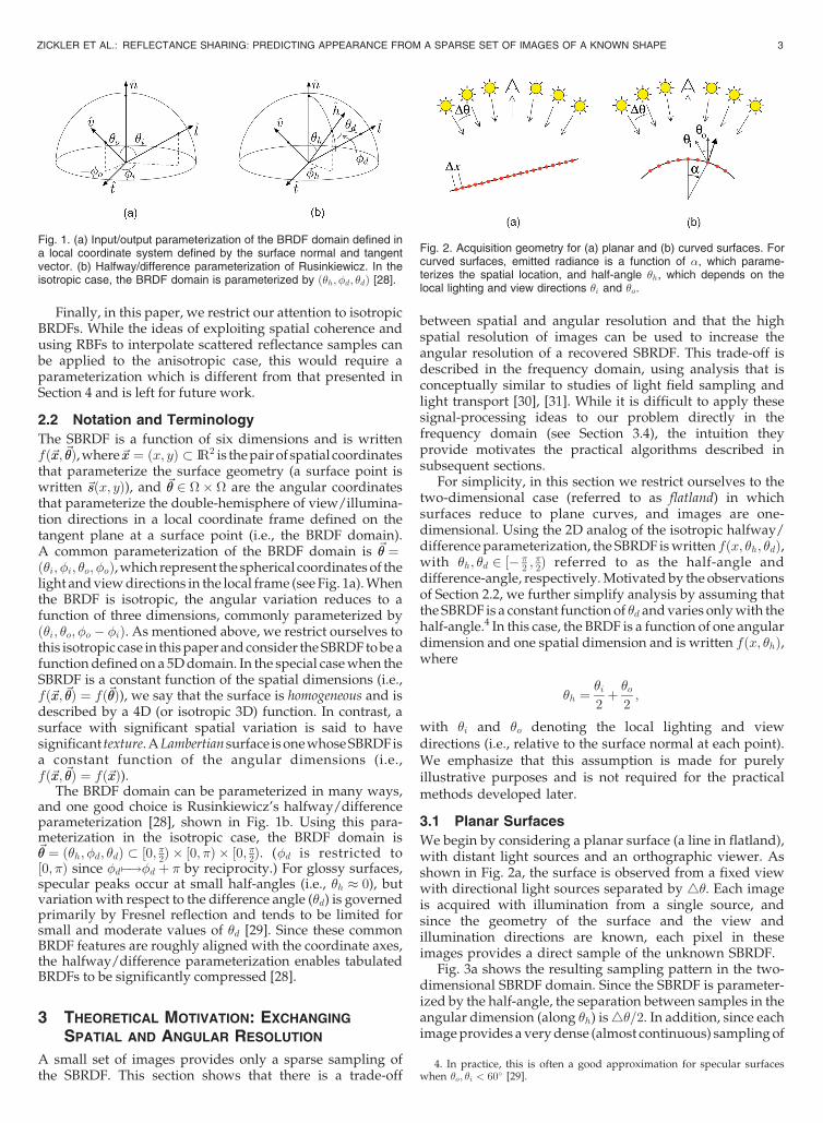
Finally, in this paper, we restrict our attention to isotropicBRDFs. While the ideas of exploiting spatial coherence andusing RBFs to interpolate scattered reflectance samples canbe applied to the anisotropic case, this would require aparameterization which is different from that presented inSection 4 and is left for future work.

2.2 Notation and Terminology

The SBRDF is a function of six dimensions and is writtenfð~xx;~��Þ, where~xx ¼ ðx; yÞ � IR2 is the pair of spatial coordinatesthat parameterize the surface geometry (a surface point iswritten ~ssðx; yÞ), and ~�� 2 �� are the angular coordinatesthat parameterize the double-hemisphere of view/illumina-tion directions in a local coordinate frame defined on thetangent plane at a surface point (i.e., the BRDF domain).A common parameterization of the BRDF domain is ~�� ¼ð�i; �i; �o; �oÞ, which represent the spherical coordinates of thelight and view directions in the local frame (see Fig. 1a). Whenthe BRDF is isotropic, the angular variation reduces to afunction of three dimensions, commonly parameterized byð�i; �o; �o � �iÞ. As mentioned above, we restrict ourselves tothis isotropic case in this paper and consider the SBRDF to be afunction defined on a 5D domain. In the special case when theSBRDF is a constant function of the spatial dimensions (i.e.,fð~xx;~��Þ ¼ fð~��Þ), we say that the surface is homogeneous and isdescribed by a 4D (or isotropic 3D) function. In contrast, asurface with significant spatial variation is said to havesignificant texture. A Lambertian surface is one whose SBRDF isa constant function of the angular dimensions (i.e.,fð~xx;~��Þ ¼ fð~xxÞ).

The BRDF domain can be parameterized in many ways,and one good choice is Rusinkiewicz’s halfway/differenceparameterization [28], shown in Fig. 1b. Using this para-meterization in the isotropic case, the BRDF domain is~�� ¼ ð�h; �d; �dÞ � ½0; �2Þ � ½0; �Þ � ½0; �2Þ. (�d is restricted to½0; �Þ since �d 7�!�d þ � by reciprocity.) For glossy surfaces,specular peaks occur at small half-angles (i.e., �h � 0), butvariation with respect to the difference angle (�d) is governedprimarily by Fresnel reflection and tends to be limited forsmall and moderate values of �d [29]. Since these commonBRDF features are roughly aligned with the coordinate axes,the halfway/difference parameterization enables tabulatedBRDFs to be significantly compressed [28].

3 THEORETICAL MOTIVATION: EXCHANGING

SPATIAL AND ANGULAR RESOLUTION

A small set of images provides only a sparse sampling ofthe SBRDF. This section shows that there is a trade-off

between spatial and angular resolution and that the highspatial resolution of images can be used to increase theangular resolution of a recovered SBRDF. This trade-off isdescribed in the frequency domain, using analysis that isconceptually similar to studies of light field sampling andlight transport [30], [31]. While it is difficult to apply thesesignal-processing ideas to our problem directly in thefrequency domain (see Section 3.4), the intuition theyprovide motivates the practical algorithms described insubsequent sections.

For simplicity, in this section we restrict ourselves to thetwo-dimensional case (referred to as flatland) in whichsurfaces reduce to plane curves, and images are one-dimensional. Using the 2D analog of the isotropic halfway/difference parameterization, the SBRDF is written fðx; �h; �dÞ,with �h; �d 2 ½� �

2 ;�2Þ referred to as the half-angle and

difference-angle, respectively. Motivated by the observationsof Section 2.2, we further simplify analysis by assuming thatthe SBRDF is a constant function of �d and varies only with thehalf-angle.4 In this case, the BRDF is a function of one angulardimension and one spatial dimension and is written fðx; �hÞ,where

�h ¼�i2þ �o

2;

with �i and �o denoting the local lighting and viewdirections (i.e., relative to the surface normal at each point).We emphasize that this assumption is made for purelyillustrative purposes and is not required for the practicalmethods developed later.

3.1 Planar Surfaces

We begin by considering a planar surface (a line in flatland),with distant light sources and an orthographic viewer. Asshown in Fig. 2a, the surface is observed from a fixed viewwith directional light sources separated by 4�. Each imageis acquired with illumination from a single source, andsince the geometry of the surface and the view andillumination directions are known, each pixel in theseimages provides a direct sample of the unknown SBRDF.

Fig. 3a shows the resulting sampling pattern in the two-dimensional SBRDF domain. Since the SBRDF is parameter-ized by the half-angle, the separation between samples in theangular dimension (along �h) is4�=2. In addition, since eachimage provides a very dense (almost continuous) sampling of

ZICKLER ET AL.: REFLECTANCE SHARING: PREDICTING APPEARANCE FROM A SPARSE SET OF IMAGES OF A KNOWN SHAPE 3

Fig. 1. (a) Input/output parameterization of the BRDF domain defined ina local coordinate system defined by the surface normal and tangentvector. (b) Halfway/difference parameterization of Rusinkiewicz. In theisotropic case, the BRDF domain is parameterized by ð�h; �d; �dÞ [28].

Fig. 2. Acquisition geometry for (a) planar and (b) curved surfaces. Forcurved surfaces, emitted radiance is a function of �, which parame-terizes the spatial location, and half-angle �h, which depends on thelocal lighting and view directions �i and �o.

4. In practice, this is often a good approximation for specular surfaceswhen �o; �i < 60� [29].

the spatial dimension, the separation between samples in that

dimension is generally very small, so that4��4x.To investigate this sampling pattern in the frequency

domain, we define the 2D Fourier transform in the

conventional way5 (and with I ¼ffiffiffiffiffiffiffi�1p

as usual),

F ð�u;�vÞ ¼Z Z

fðu; vÞe�2�I�uue�2�I�vv du dv;

where we are interested in the spatially varying BRDF

fðx; �hÞ with Fourier transform F ð�x;��Þ. Sampling in the

spatial domain is represented by multiplication by the

comb function

fsampledðx; �hÞ ¼ fðx; �hÞXn1;n2

�ðx� n14xÞ�ð�h � n24�=2Þ;

where n1 and n2 are integers. The Fourier transform of this

sampled signal is obtained by convolution with a comb

function, which yields

Fsampledð�x;��Þ ¼Xn1;n2

F �x �2�n1

4x ;�� 4�n2

4�

� �:

In the frequency domain, the sampling process produces

shifted replicas of the SBRDF spectrum. These replicas are

at intervals of 2�=4x spatially and 4�=4� in the angular

dimension. This is shown in Fig. 3b, assuming a sufficiently

band-limited SBRDF.In order to synthesize novel images of the surface (i.e., to

predict its appearance), the SBRDF must be reconstructed

from its samples. Accurate reconstruction that avoids aliasing

during image synthesis requires a sampling rate satisfying

the Nyquist conditions. Letting �maxx and �max

� denote the

spatial and angular bandwidths6 of the SBRDF, we require

�maxx <

�

4x �max� <

2�

��: ð1Þ

These sampling conditions are quite intuitive. The maximumspatial frequency of the surface cannot exceed the pixelresolution of the camera, and the maximum angularfrequency (which is a measure of the surface “shininess”)cannot exceed the sampling resolution of the light sources.Furthermore, the optimal reconstruction filter in the Fourierdomain is the elongated box shown in red in Fig. 3b, whichsimply band-limits differently in the spatial and angulardimensions according to the relations above. Intuitively,when the SBRDF is reconstructed, each pixel is treatedseparately, and the “sharpness” of the recovered specularhighlights is bounded by the number of light source locationsas noted in previous nonparametric acquisition methods [11],[12], [13]. This result is the foundation for the analysis ofcurved surfaces, discussed next.

3.2 Curved Surfaces

Acquisition for curved surfaces (plane curves in flatland) isshown in Fig. 2b. Assuming constant curvature, we canparameterize the spatial dimensionxby angle�, since there isa linear relationship between the two. The goal is toreconstruct the spatially varying BRDF fð�; �hÞ from thesamples obtained from a set of images similar to those in theprevious section.

To derive an expression for �h in terms of the globalpositions of the camera and light source (�c and �l), we usethe convention that � is positive in the direction shown inFig. 2b. Then,

�h ¼�l � �þ �c � �

2¼ �l þ �c

2� � ¼ h� �;

where h ¼ ð�l þ �cÞ=2 can be thought of as the “global half-angle.” Thus, we can reparameterize7 the spatially varyingBRDF:

fð�; �hÞ ¼ fð�; h� �Þ:

Fig. 4a depicts the resulting sampling pattern in the SBRDFdomain. Assuming uniformly spaced samples on the surface(but see Section 3.4), the spacing between samples is denoted4� and is analogous to 4x in the planar case. The spacingbetween successive global half-angles (4h) is simply 4�=2,just as in the planar case, and as before, 4h�4�. Thesampling pattern is now rotated, however, as shown in Fig. 4a.In this figure, each image corresponds to a line with negativeslope and a y-intercept at h. Along each of these image lines,the net sample spacing is

ffiffiffi2p4�. The perpendicular distance

between lines is4h=ffiffiffi2p¼ 4�=ð2

ffiffiffi2pÞ. As we now show, this

shearing pattern leads to interesting consequences in thefrequency domain.

In the SBRDF domain, the continuous signal is multi-plied by a comb function with the pattern shown in Fig. 4a.The effect in the frequency domain is described byconvolution with a similar comb function, but with differentperiods along the two axes. To determine these periods, we


5. In general, one would need to use a Fourier series for periodic angularvalues and a continuous infinite domain for the spatial component.However, the core analysis is not affected by these issues and, in whatfollows, we omit the limits of integration, allowing whichever interpretationis more convenient for the reader.

6. We assume rectangular bandlimits for simplicity. There does notappear to be a physical basis for assuming, for example, an ellipticalspectrum, nor would it significantly affect the results.

7. It is important to note that while the half-angle parameterization ishelpful in representing real BRDFs, it is not critical to enable reflectancesharing. For example, if the SBRDF were a function of fð�; �iÞ instead offð�; �hÞ, we would simply write �i ¼ �l � �, with h replaced by �l in (2),leading to essentially the same form.

Fig. 3. (a) Spatial/angular sampling pattern for SBRDF acquisition usinga planar surface. Sample spacing is high along the spatial dimension(4x) but lower along the angular dimension (4�=2). (b) Fourierspectrum of the sampled SBRDF. Green rectangles correspond to theoriginal spectrum, which is replicated along spatial and angularfrequencies. The red box in the middle corresponds to the idealreconstruction filter.

note that the sampling pattern in Fig. 4a is obtained byrotating the planar sampling pattern (Fig. 3a) by þ45�. Thelinear transformation theorem [32] then tells us that theFourier transform of the planar comb function will also berotated by þ45�, and that the sampling rates will be scaledappropriately. More formally, the comb function in thefrequency domain is (with m1 and m2 integers),

COMBðu; vÞ ¼ 4ffiffiffi2p

� m1

4�uffiffiffi2p þ vffiffiffi

2p

� �

þffiffiffi2p

� m2

4� � uffiffiffi2p þ vffiffiffi

2p

� �;

ð2Þ

and the Fourier transform of the sampled curved-surfaceSBRDF is

Fsampledð��;��Þ ¼Xm1;m2

F �� 4�m1

4� þ�m2

4� ;�� 4�m1

4� ��m2

4�

� �:ð3Þ

To provide some intuition, consider the set of replicaswith m2 ¼ 0. In this case, the replicas indexed by m1 lie on a45� line with a sample spacing of 4

ffiffiffi2p

�=4� as calculated

earlier. Replicas with m2 6¼ 0 lie on parallel lines, and sincethe spatial sampling rate is typically large relative to theangular sampling rate, these lines are well separated. Thispattern of replicas—analogous to Fig. 3b—is shown inFig. 5a. Note from this figure that the conditions for alias-free synthesis remain similar to the planar case, as does theoptimal reconstruction filter. In particular, given samplingrates 4� and 4� the conditions for alias-free imagesynthesis are

�max� <

�

24� �max� <

2�

4� : ð4Þ

3.3 Reflectance Sharing

As in the planar case, the bounds in (4) suggest that we canaccurately recover an SBRDF from a small number of images(i.e., a large 4�) provided that there is only low-frequencyvariation in the angular dimension. A synthetic example of anobject that satisfies this criteria is shown in the inset in Fig. 5a,where even though there is high-frequency spatial variation(significant texture), the reflectance at each point is quitediffuse (i.e., it is nearly Lambertian).

What is very different from the planar case is that inaddition to diffuse surfaces like that shown in Fig. 5a, we canalso recover reflectance like that shown in the inset of Fig. 5b.This surface is characterized by low-frequency spatialvariation (little texture) and high-frequency angular variation(sharp highlights). The frequency-domain effects of samplingthis type of SBRDF are depicted in the graph in Fig. 5b. Thespectrum of the SBRDF is a rectangle that is elongated in theangular frequency dimension, and the optimal reconstruc-tion filter (shown in red) maintains this shape. The limits onthe SBRDF spectrum for alias-free synthesis are:

�max� <

2�

4� �max� <

�

24� : ð5Þ

Here, the maximum spatial bandwidth (i.e., in the�-dimension) is constrained by the separation of light sourcedirections4�, while the angular bandwidth is constrained bythe spatial sampling 4�. This is in direct opposition to thelimits of (4), and it means, for example, that we can recover


Fig. 4. (a) Sampling pattern in the SBRDF domain for acquisition using acurved surface. Unlike the planar case of Fig. 3a, the sampling pattern isoriented at 45� to the axes, as per Section 3.2. Spacing in the twodirections is

ffiffiffi2p4� and 4�=ð2

ffiffiffi2pÞ with 4��4�. (b) The comb

function (in the frequency domain) is described by (2). Sampling theSBRDF according to (a) corresponds to convolution in the frequencydomain by this comb function, which has the same rotated form.

Fig. 5. Fourier transforms of sampled SBRDFs obtained from observations of curved surfaces. Green rectangles correspond to the originalfrequency spectra for predominantly (a) diffuse and (b) specular reflectance, and central red rectangles are the ideal reconstruction filters. Insetscontain examples of diffuse and specular surfaces under directional illumination.

very sharp specular highlights from a single image (withdense spatial sampling) like that shown in Fig. 5b. Theoptimal reconstruction filter is a low-pass filter with a smallcutoff frequency in the spatial dimension, which in theSBRDF domain, corresponds to an averaging over a largespatial extent. We refer to this averaging process as reflectancesharing, since it enables the use of the high spatial resolutionavailable in images to increase the angular resolution of therecovered reflectance function.

The limits in (5) also indicate that the recovered spatialfrequencies are constrained by the separation of lightsources. Given only a single image, for example, the spatialbandwidth is limited to zero (since 4�!1), and we canonly recover accurate reflectance for homogeneous surfaceswithout texture. Information about spatial variation orinhomogeneity in the SBRDF can only be obtained withadditional images that provide observations of specularhighlights in multiple regions of the surface.

This spatial/angular trade-off can be further understoodby noting that the product of the bounds on bandwidth inthe spatial and angular dimensions is always given by

�max� �max

� <�2

4�4� : ð6Þ

This expression tells us that we can recover high SBRDFfrequencies in one of the spatial or angular dimensions from asparse set of images, but not both simultaneously. Conven-tional SBRDF acquisition methods [11], [12], [13] present onlyone possible approach. They treat each spatial sampleseparately and provide very high spatial resolution withlimited angular resolution. By contrast, we seek to sharereflectance spatially, estimating an SBRDF with high angularfrequency at the cost of a decrease in spatial resolution.

It is also interesting to note that if the surface curvaturek is explicitly represented through the relation � ¼ kx, thebandwidth limits are given by �max

� < 2�k=4� and �max� <

�=k4� (and (6) still holds). Thus, as long as there is somecurvature (k > 0), we can recover very high angularfrequencies, provided the spatial frequencies are stronglybandlimited.

Finally, we emphasize that glossy reflectance like that inFig. 5b generally cannot be recovered from sparse images inthe planar case.8 Indeed, given the sampling pattern ofFig. 3a, the repeated spectra for a glossy surface wouldoverlap. It is the surface curvature that causes the rotatedpatterns in Fig. 3, which in turn allows the recovery of high-frequency angular reflectance from sparse images.

3.4 Images and Irregular Sampling

The analysis of this section relies on the assumption thatsamples in the spatial dimension are uniformly spaced onthe surface. For image-based data, however, samples areuniformly spaced on the image-plane, and for curved objectsthis leads to a very irregular sampling of the object’ssurface. Thus, while Fourier analysis provides insight andmotivation for the reflectance sharing approach, it isdifficult to implement a practical frequency-based methodusing these ideas. Instead, the remainder of this paper

develops a scattered data interpolation method using radialbasis functions, with weights to trade off the extent ofsharing in the spatial and angular dimensions. In thecontext of the preceding analysis, this is analogous tobuilding a reconstruction filter by selecting appropriate cut-off frequencies in the spatial and angular dimensions.

4 SBRDF PARAMETERIZATION

At the core of our approach is the interpolation of scattereddata in multiple dimensions, the success of which dependson how the SBRDF is parameterized. The previous sectionused the special case of plane curves to describe how theassumption of angular compressibility and the halfway/difference parameterization are important for correctlyframing the problem. Inspired by this theory, this sectionconsiders the three-dimensional case and introduces a newparameterization for the angular dimensions of an SBRDF.Based on this parameterization, our interpolation techniqueis discussed in Sections 6 and 7.

The halfway/difference BRDF parameterization of Rusin-kiewicz [28] was described in Section 2.2. The existence ofsingularities at �h ¼ 0 and �d ¼ 0 and the required periodicity(�d 7�!�d þ �) make this parameterization unsuitable formost interpolation techniques, and in order to address this,we define a mapping ð�h; �d; �dÞ 7�!ðu; v; wÞ, as

ðu; v; wÞ ¼ sin �h cos 2�d; sin �h sin 2�d;2�d�

� �; ð7Þ

which is shown in Fig. 6. This mapping defines a newparameterization for the angular dimensions of an SBRDF(i.e., the BRDF domain.) It eliminates the singularity at �h ¼0 and ensures that the BRDF fðu; v; wÞ satisfies reciprocity.In addition, the mapping is such that the remainingsingularity occurs at �d ¼ 0, where the light and viewdirections are equivalent. This is desirable because thisconfiguration is difficult to create in practice, which makesit unlikely to occur during acquisition. During synthesis,however, it must be handled with care.

4.1 Considerations for Image-Based Acquisition

As mentioned previously, the halfway/difference parame-terization increases compression rates since commonfeatures such as specular and retro-reflective peaks arealigned with the coordinate axes [28]. The modifiedparameterization of (7) maintains this property, sincespecular events cluster along the w-axis, and retro-reflectivepeaks occur in the plane w ¼ 0.

These parameterizations are useful for image-based datafor an additional reason: They separate the sparsely and


8. Again, using perspective cameras and near-field illumination, angularinformation can be obtained in the planar case [17].

Fig. 6. The mapping in (7) creates a BRDF parameterization suitable forinterpolation. The BRDF fðu; v; wÞ is guaranteed to satisfy reciprocity,the parameterization is defined for all values of �h, BRDF samples froma single image lie on a plane of constant w, and specular events areclustered near the w-axis, enabling significant compression.

densely sampled dimensions of the BRDF. (Marschner’sparameterization [33] also shares this property.) To see this,note that for orthographic projection and distant light-ing—or more generally, when scene relief is relativelysmall—a single image of a curved surface provides BRDFsamples lying in a plane of constant �d, since this angle isindependent of the surface normal. Indeed, for the flatlandcase of Section 3.2, the difference angle is

�d ¼�c � �� l þ �

2¼ �c � �l

2; ð8Þ

which depends on the global camera and light positions but

not the spatial location �.While each (orthographic) image provides only one

sample of the �d dimension, it represents a nearly continuoussampling of �h and �d. As a result, a set of images providesdense sampling of ð�h; �dÞ but only as many samples of �d asthere are images.9 Conveniently, this irregular samplingobtained from image-based data corresponds well with thebehavior of general BRDFs, which vary slowly in the sparselysampled �d-dimension, especially when �d is small [29]. At thesame time, by imaging curved surfaces, we ensure that thesampling rate of the half-angle �h is high enough to accuratelyrecover the high-frequency variation (e.g., due to specularhighlights) that is generally observed in that dimension.

5 SCATTERED DATA INTERPOLATION

Recall that our goal is to estimate a continuous SBRDFfð~xx;~��Þ from a set of samples fi 2 IR5 drawn from images ofa surface with known geometry. Our task is complicated bythe fact that, as discussed in Section 3.4, the input samplesare very nonuniformly distributed.

There are many methods for interpolating scattered datain this relatively high-dimensional space, but for ourproblem, interpolation using radial basis functions providesthe most attractive choice. Given a set of samples, an RBFinterpolant is computed by solving a linear system ofequations, and the existence and uniqueness is guaranteedwith few restrictions on the sample points. Thus, unlikehomogeneous BRDF representations such as sphericalharmonics, Zernike polynomials, wavelets, and the basisof Matusik et al. [15], an RBF representation does notrequire a local preprocessing step to resample the inputdata at regular intervals.

Additionally, for a fixed number of samples, the requiredcomputation and the resulting size of an RBF representationgrow relatively slowly as the dimension increases. This is incontrast to methods such as piecewise polynomial splines(e.g., [34]) and local methods like polynomial regression (e.g.,[14]) and the push/pull algorithm of Gortler et al. [24]. Thesealternative methods require either a triangulation of thedomain or a tabulation of function values, both of whichbecome computationally prohibitive in high dimensions.(Jaroszkiewicz and McCool [20]handle this by approximatingthe high-dimensional SBRDF by a product of 2D functions,each of which is triangulated independently.)

5.1 Radial Basis Functions

To briefly review RBF interpolation (see, e.g., [35], [36]),consider a general function gð~xxÞ; ~xx 2 IRd from which we haveN samples fgig at sample points f~xxig. This function isapproximated by a sum of a low-order polynomial and a set ofscaled, radially symmetric basis functions centered at thesample points:

gð~xxÞ � ~ggð~xxÞ ¼ pð~xxÞ þXNi¼1

�i ðk~xx�~xxikÞ; ð9Þ

where pð~xxÞ is a polynomial of order n or less, : IRþ !IR is a continuous function, and k � k is the Euclideannorm. The sample points ~xxi are referred to as centers andthe RBF interpolant ~gg satisfies the interpolation condi-tions ~ggð~xxiÞ ¼ gð~xxiÞ.

Given a choice of n, an RBF , and a basis for thepolynomials of order n or less, the coefficients of theinterpolant are given by the solution of the linear system

� PP> 0

� �~��~cc

� �¼ ~gg

0

� �; ð10Þ

where �ij ¼ ðk~xxi �~xxjkÞ, ~��i ¼ �i,~ggi ¼ gi, Pij ¼ pjð~xxiÞ, wherefpjg are the polynomial basis functions, and ~cci ¼ ci are thecoefficients in this basis of the polynomial term in ~gg. Thissystem is invertible (and the RBF interpolant is uniquelydetermined) in arbitrary dimensions for many choices of ,with only mild conditions on n and the locations of the datapoints [37], [38].

In practical cases, the samples fgig are affected by noise,and it is desirable to allow the interpolant to deviate fromthe data points, balancing the smoothness of the interpolantwith its fidelity to the data. This is accomplished byreplacing � in (10) with �� NI, where I is the identitymatrix and � is a stiffness parameter. Further details areprovided by Wahba [39].

In many cases, we can benefit from using radially asym-metricbasisfunctionswhicharestretchedincertaindirections,and here we use them to: 1) control the trade-off betweenspatial and angular resolution, and 2) manage the irregularityin our sampling pattern. (Recall that the ðu; vÞdimensions aresampled almost continuously while we have only as manysamples ofwas we have images.) Following Dinh et al. [40], anasymmetric radial function is created by scaling the Euclideandistance in (9) so that the basis functions become

ðkMð~xx�~xxiÞkÞ; ð11Þ

where M 2 IRd�d. In our case, we choose M to be a diagonalmatrix whose entries reflect the expected relative rates ofchange in the spatial and angular dimensions, and therelative sampling rates of the three angular dimensions.(See Sections 6 and 7.)

When the number of samples is large (N > 10; 000),solving (10) requires care and can be difficult—or impossi-ble—using direct methods. This limitation has beenaddressed quite recently, and iterative fitting methods [41]and fast multipole methods (FMMs) for efficient evaluation[42] exist for many choices of in many dimensions. Insome cases, solutions for systems with over half a millioncenters have been reported [43]. The next sections includeinvestigations of the number of RBF centers required to


9. The orthographic/directional case is considered for illustrativepurposes; it is not required by the method.

accurately represent image-based reflectance data, and wefind this number to be sufficiently small to allow the use ofdirect methods.

6 HOMOGENEOUS SURFACES

This section applies RBF interpolation to homogeneoussurfaces, where we seek to estimate a global BRDF that isnot spatially varying. The derived representation may beuseful for interpolating image-based BRDF data [10], [14],[15]. The theoretical analysis in Section 3 shows that thevariation with respect to the half-angle can be estimated froma single image of a homogeneous, curved surface. While moreimages are needed to acquire the full BRDF, this sectionshows that a sparse set often suffices.

As discussed in Section 4, for homogeneous BRDF data,

reflectance is a function of three dimensions, ðu; v; wÞ. In IR3, a

good choice for is the linear (or biharmonic) RBF, ðrÞ ¼ r,with n ¼ 1, since in this case, the interpolant from (10) exists

for any noncoplanar data, is unique, minimizes a general-

ization of the thin-plate energy, and is therefore the smoothest

in some sense [37], [43]. The BRDF is expressed as

~ffð~��Þ ¼ c1 þ c2uþ c3vþ c4wþXNi¼1

�ik~�� ~��ik; ð12Þ

where ~��i ¼ ðui; vi; wiÞ represents a BRDF sample pointobtained from the input images, and ~�� and ~cc are found bysolving (10). As discussed in the previous section, we canbenefit from the use of radially asymmetric basis functions,and for homogeneous BRDF data, this is accomplished usingM ¼ diagð1; 1;mwÞ. For mw < 1, the basis functions areelongated in the w dimension, which is appropriate sinceour sampling rate is much lower in that dimension. Theappropriate value of this parameter depends on the angulardensity of the input images, and empirically we find thattypical values for mw are between 0.1 and 0.5.

As a practical consideration, since each pixel represents asample point~��i, even with modest image resolution, using allavailable samples as RBF centers is computationally prohi-bitive. Much of this data is redundant, however, and anaccurate BRDF representation can be achieved using only asmall fraction of these centers. A sufficient subset of centerscould be chosen using knowledge of typical reflectancephenomena. (To represent sharp specular peaks, for example,RBF centers are generally required near �h ¼ 0.) Alterna-tively, Carr et al. [43] present an effective greedy algorithm forchoosing this subset without assuming prior knowledge, anda slightly modified version of the same algorithm is appliedhere. The procedure begins by randomly selecting a smallsubset of the sample points~��i and fitting an RBF interpolant tothese. Next, this interpolant is evaluated at all sample pointsand used to compute the radiance residuals, "i ¼ ðfi � ~ffð~��iÞÞ cos �i, where �i is the angle between the surface normal atthe sample point and the illumination direction. Finally,points where "i is large are appended as additional RBFcenters, and the process is repeated until the desired fittingaccuracy is achieved.

It should be noted that an algorithmic choice of centerlocations could increase the efficiency of the resultingrepresentation, since center locations would not necessarilyneed to be stored for each material. However, this would

require assumptions about the function being approxi-mated, and here, we choose to emphasize generality overefficiency by using the greedy algorithm.

6.1 Evaluation

To evaluate the BRDF representation in (12), we performcomparisons to both parametric BRDF models and to anonlinear basis (the isotropic Lafortune model [44]). Themodels are fit to synthetic images of a sphere, and theiraccuracy is measured by their ability to predict theappearance of the sphere under novel conditions. (Otherrepresentations such as wavelets and the Matusik bases areexcluded from this comparison because they require dense,uniform samples.)

The input images simulate data from image-based BRDFmeasurement systems like those in [10], [14], [15]. They areorthographic, directional-illumination images with a resolu-tion of 100� 100, and are generated such that �d is uniformlysampled in ½0; �2. The accuracy of the recovered models ismeasured by the relative RMS radiance error over 21 im-ages—also uniformly spaced in �d—that are not used asinput. For these simulations, we use both specular and diffusereflectance, one drawn from measured data (the metallic-blueBRDF, courtesy of Matusik et al. [15]), and the other generatedusing the physics-based Oren-Nayar model [9].

Fig. 7 shows the accuracy of increasingly complex RBF andLafortune representations fit to 10 input images. Thecomplexity of the RBF representation is measured by thenumber of centers selected by the greedy algorithm, and thatof the Lafortune model is measured by the number ofgeneralized cosine lobes. An unusually large number of lobesare shown (two or three lobes is typical) so that the resultingLafortune and RBF representations have comparable degreesof freedom. It is important to note, however, that the size ofeach representation is different for equivalent complexities;an N-lobe isotropic Lafortune model requires 3N þ 1 para-meters, while an N-center RBF interpolant requires 4N þ 4.

Since the basis functions of the Lafortune model are

designed for representing BRDFs and are therefore em-

bedded with knowledge of general reflectance behavior, they

provide a reasonably good fit with a small number of lobes.

For example, a 6-lobe Lafortune model (19 parameters) yields


Fig. 7. Accuracy of the RBF representation as the number of centers isincreased using a greedy algorithm. The input is 10 images of a spheresynthesized using the metallic-blue BRDF measured by Matusik et al.[15]. This is compared to the isotropic Lafortune representation [44] withan increasing number of lobes. Less than 1,000 centers are sufficient torepresent the available reflectance information using RBFs, whereas thelimited flexibility of the Lafortune basis and the existence of local minimain the nonlinear fitting process limit the accuracy of the Lafortunerepresentation. (See text for details.)

the same RMS error as a 300-center RBF model (1,204 para-

meters). In addition to being compact, the Lafortune model

has the advantage of being more suitable for direct rendering

[5]. But, the accuracy of this representation is fundamentally

limited; the lack of flexibility and the existence of local

minima in the required nonlinear fitting process prevent the

Lafortune model from accurately representing the reflectance

information available in the input images.In contrast, RBFs provide a general linear basis and with a

sufficient number of centers, they can represent any“smooth” function with arbitrary accuracy (e.g., [36]). Here,the RBF representation converges with less than 1,000 centers,suggesting that only a small fraction of the available centersare needed to summarize the reflectance information in the10 input images.

Similar conclusions are drawn from a second experimentin which we investigate the accuracy of these and otherrepresentations with a fixed level of complexity and anincreasing number of input images. Results are shown inFigs. 8 and 9 for predominantly specular and diffusereflectance. (Here, six lobes are used in the Lafortunerepresentation since the results do not change significantlywith additional lobes.) Since RMS error is often not anaccurate perceptual metric, these figures also includesynthetic spheres rendered with the recovered models. Thisexperiment demonstrates the flexibility of the RBF represen-tation, which captures both the Fresnel effects in Fig. 8 and theretro-reflection in Fig. 9. Parametric models do not typicallyafford this flexibility—while it may be possible to find aparametric model that fits a specific BRDF quite well, it is verydifficult to find a model that accurately fits general BRDFs.

7 INHOMOGENEOUS SURFACES

The previous section suggests that RBFs can provide auseful representation for homogeneous BRDFs. In thissection, we show that essentially the same representation

can be used to handle spatially varying reflectance as well.It enables the exchange between spatial and angularresolution (as described in Section 3), and drasticallyreduces the number of required input images. We beginby assuming that the 5D SBRDF varies slowly in the spatialdimensions and, in the next section, we show how this canbe generalized to handle rapid spatial variation in terms ofa multiplicative albedo or texture.

In the homogeneous case, the BRDF is a function of threedimensions, and the linear RBF ðrÞ ¼ r yields a uniqueinterpolant that minimizes a generalization of the thin-plateenergy. Although optimality cannot be proven, this RBF hasshown to be useful in higher dimensions as well since itprovides a unique interpolant in any dimension for any n[35]. In the spatially varying case, the SBRDF is a functionof five dimensions, and we let~qq ¼ ðx; y; u; v; wÞ be a point inits domain. Using the linear RBF with n ¼ 1, the SBRDF isgiven by

~ffð~qqÞ ¼ pð~qqÞ þXNi¼1

�ik~qq �~qqik; ð13Þ

where pð~qqÞ ¼ c1 þ c2xþ c3yþ c4uþ c5vþ c6w.We can use any parameterization of the surface ~ss, and

there has been significant recent work on determininggood parameterizations for general surfaces (e.g., [46],[47]). The ideal surface parameterization is one thatpreserves distance, meaning that k~xx1 �~xx2k is equivalentto the geodesic distance between ~ssð~xx1Þ and ~ssð~xx2Þ. Forsimplicity, here we treat the surface as the graph of afunction, with ~ssðx; yÞ ¼ ðx; y; sðx; yÞÞ; ðx; yÞ � ½0; 1 � ½0; 1.

The procedure for recovering the parameters in (13) is

almost exactly the same as in the homogeneous case. The

coefficients of ~ff are found by solving (10) using a subset of the

input SBRDF samples and this subset is chosen using a greedy

algorithm. Radially asymmetric basis functions are realized

using M ¼ diagðmxy;mxy; 1; 1;mwÞ, where mxy controls the


Fig. 8. Top: Error in the estimated BRDF for an increasing number ofimages of a metallic-blue sphere. As the number of images increases,the RBF representation (with 1,000 centers) approaches the true BRDF,whereas the isotropic Ward model [45] and the Lafortune representationare too restrictive to provide an accurate fit. Bottom: Synthesizedimages using the three BRDF representations estimated from 12 inputimages, where the angle between the source and view directions is 140�.

Fig. 9. Top: Error in the estimated BRDF for an increasing number ofinput images of a diffuse Oren-Nayar sphere. Again, the 1,000-centerRBF representation approaches the true BRDF, whereas the Lafortuneand Lambertian BRDF models are too restrictive to accurately representthe data. Bottom: Synthesized images comparing the three BRDFrepresentations estimated from 12 input images, where the anglebetween the source and view directions is 10�.

exchange between spatial and angular reflectance informa-

tion. When mxy 1, the basis functions are elongated in the

spatial dimensions, and the recovered reflectance function

approaches a single BRDF (i.e., a homogeneous representa-

tion) with rapid angular variation. Whenmxy � 1, we recover

a near-Lambertian representation in which the BRDF at each

point approaches a constant function of~��. Appropriate values

ofmxy depend on the choice of surface parameterization and

we found typical values to be between 0.2 and 0.4 for the

examples in this paper.

7.1 Evaluation

The SBRDF representation of (13) can be evaluated using

experiments similar to those for the homogeneous case.

Here, spatial variation is simulated using images of a

hemisphere with a Cook-Torrance BRDF [8] with a linearly

varying roughness parameter. Five images are shown in

Fig. 10 and they demonstrate how the highlight sharpens

from left to right across the surface.The graph in Fig. 10 shows the accuracy of the recovered

SBRDF as a function of the number of RBF centers when it is

fit to images of the hemisphere under 10 uniformly

distributed illumination directions. The error is computed

over 40 images that are not used as input. Fewer than

2,000 centers are needed to accurately represent the spatial

reflectance information available in the input images, which

is a reasonably compact representation requiring roughly

12,000 parameters. For comparison, an SBRDF representation

for a 10,000-vertex surface consisting of two unique Lafortune

lobes at each vertex is roughly five times as large.Fig. 11 contrasts reflectance sharing with conventional

methods that interpolate only in the angular dimensions,

estimating a separate BRDF at each point. This “no sharing”

approach is used by Matusik et al. [13] and is similar in spirit

to Wood et al. [11], who also estimate a unique view-

dependent function at each point. (In this discussion, angular

interpolation in the BRDF domain is assumed to require

known geometry, which is different from lighting interpola-

tion (e.g., [12]) that does not. For the particular example in

Fig. 11, however, the “no sharing” result can be obtainedwithout geometry since it is a special case of fixed viewpoint.)

For both the reflectance sharing and “no sharing” cases,the SBRDF is estimated from images with fixed viewpointand uniformly distributed illumination directions such asthose in Fig. 10, and the resulting SBRDF is used to predict theappearance of the surface under novel lighting. The top frameof Fig. 11 shows the actual appearance of the hemisphereunder five novel conditions, and the lower frames show thereflectance sharing and “no sharing” results obtained fromincreasing numbers of input images. Note that many othermethods—most notably that of Lensch et al. [16]—areexcluded from this comparison because they require theselection of a specific parametric model and, therefore, sufferfrom the limitations discussed in Section 6.

In this example, reflectance sharing reduces the number ofrequired input images by more than an order of magnitude.Five images are required for good visual results using theRBF representation, whereas at least 150 are needed if onedoes not exploit spatial coherence. Fig. 11 also shows howdifferently the approaches degrade with sparse input.Reflectance sharing provides a smooth SBRDF whoseaccuracy gradually decreases away from the convex hull ofinput samples. (For example, the sharp specularity on theright of the surface is not accurately recovered when only twoinput images are used.) In contrast, when interpolating onlyin the angular dimensions, a small number of imagesprovides only a small number of reflectance samples at eachpoint; and as a result, severe “ghosting” occurs when the


Fig. 10. Top: Accuracy of the SBRDF recovered by reflectance sharingusing the RBF representation in (13) as the number of centers isincreased using a greedy algorithm. The input is 10 synthetic images ofa hemisphere (five of which are shown) with linearly varying roughness.

Fig. 11. Estimating the spatially varying reflectance function from asparse set of images. Top frame: five images of a hemisphere underillumination conditions not used as input. Middle frame: appearancepredicted by reflectance sharing with two and five input images. (Theinput images are shown in Fig. 10; the two left-most images are used forthe two-image case.) Bottom frame: appearance predicted by inter-polating only in the angular dimensions with 5, 50, and 150 input images.At least 150 images are required to obtain a result comparable to thefive-image reflectance sharing result.

surface is illuminated by high-frequency environments likethe directional illumination shown here. This is easy tounderstand in terms of the theoretical analysis in Section 3. Ineffect, angular interpolation uses a filter of the form shown inFig. 5a to reconstruct a spectrum of the form of Fig. 5b, whichleads to considerable aliasing.

Even when the input images are captured from a single

viewpoint, our method recovers a full SBRDF and, as shown

in Fig. 12, view-dependent effects can be predicted. This is

made possible by spatial sharing (since each surface point is

observed from a unique view in its local coordinate frame)

and by reciprocity (since we effectively have observations in

which the view and light directions are exchanged).

8 GENERALIZED SPATIAL VARIATION

This section considers generalizations of the radial basis

function SBRDF model by softening the requirement for

spatial smoothness and uses it to model the appearance of a

human face. Since our estimate of spatially varying

reflectance allows us to synthesize images from any lighting

direction and view, an approach such as this may

eventually enable lighting and pose-insensitive recognition

that requires only a few input images for enrollment.Rapid spatial variation can be handled using a multi-

plicative albedo or texture as in

fð~xx;~��Þ ¼ að~xxÞdð~xx;~��Þ;

where að~xxÞ is an albedo map for the surface and dð~xx;~��Þ is asmooth function of five dimensions. As an example,consider the human face in Fig. 13a. The function að~xxÞaccounts for rapid spatial variation due to pigment changes,while dð~xx;~��Þ models the smooth spatial variation thatoccurs as we transition from a region where skin hangsloosely (e.g., the cheek) to where it is taut (e.g., the nose).

In some cases, it is advantageous to express the SBRDF as alinear combination of 5D functions. For example, Sato et al. [6]and many others use the dichromatic model of reflectance[48] in which the BRDF is written as the sum of an RGB diffusecomponent and a scalar specular component that multipliesthe source color. We employ the dichromatic model here, andcompute the emitted radiance using

Ikð~xx;~��Þ ¼ sk akð~xxÞdkð~xx;~��Þ þ gð~xx;~��Þ� �

cos �i; ð14Þ

where ss ¼ fskgk¼RGB is an RGB unit vector that describes

the color of the light source. In (14), a single function g is

used to model the specular reflectance component, while

each color channel of the diffuse component is modeled

separately. This is significantly more general than the usual

assumption of a Lambertian diffuse component, and it can

account for changes in diffuse color as a function of ~��, such

as the desaturation of the diffuse component of skin at large

grazing angles witnessed by Debevec et al. [12].

Finally, although not used in our examples, more general

spatial variation can be modeled by dividing the surface

into a finite number of regions, where each region has

spatial reflectance as described above. This technique is

used, for example, in [16], [20].

8.1 Data Acquisition and SBRDF Recovery

For real surfaces, we require geometry and a set of images

taken from known viewpoint and directional illumination.

In addition, to estimate the separate diffuse and specular

reflection components in (14), the input images must be

similarly decomposed. Specular/diffuse separation can be

performed in many ways (e.g., [6], [49]), one of which uses

linear polarizers on both the camera and light source. Two

exposures are captured for each view/lighting configura-

tion, one with the polarizers aligned (to observe the sum of

specular and diffuse components), and one with the source

polarizer rotated by 90� (to observe the diffuse component

only). The specular component is then given by the

difference between these two exposures. (See, e.g., [50].)

Geometry can also be recovered in a number of different

ways. One possibility is photometric stereo, since under the

right conditions, it provides the precise surface normals

required for reflectometry. Fig. 13 shows an example of a

decomposed image along with the corresponding geome-

try, which is recovered by applying Lambertian photo-

metric stereo to a set of diffuse (ideally Lambertian) images

like that shown in the left of the figure.

Given the geometry and a set of decomposed images, the

representation in (14) can be fit as follows: First, the effects

of shadows and shading are computed, shadowed pixels

are discarded, and shading effects are removed by dividing

by cos �i. The RGB albedo að~xxÞ in (14) is estimated as the

median of the diffuse samples at each surface point and

normalized diffuse reflectance samples are computed by

dividing by að~xxÞ. The resulting normalized diffuse samples

are used to estimate the three functions dkð~xx;~��Þ in (14) using

the RBF techniques described in Section 5.1. The samples

from the specular images are similarly used to compute g.


Fig. 12. Actual and predicted appearance of the hemisphere under fixed

illumination and changing view. Given five input images from a single

view (Fig. 10), the reflectance sharing method recovers a full SBRDF,

including view-dependent effects.

Fig. 13. (a) and (b) Diffuse and specular components of a single input

view. (c) Geometry for SBRDF recovery and image synthesis.

8.2 Image Synthesis

In order to synthesize images under arbitrary view and

illumination, the SBRDF coordinates ~qq at each surface point

are determined by the spatial coordinates ~xx, the surface

normal, and the view and lighting directions. The radiance

emitted from that point toward the camera is then given by

(14). Because (14) involves sums over a large number of RBF

centers for each pixel, image synthesis can be slow. This

process can be accelerated, however, using computer

graphics techniques, including programmable graphicshardware and image precomputation.

Hardware Rendering Using the GPU. Equation (14) is

well suited to implementation in graphics hardware

because the same calculations are done at each pixel. For

example, a vertex program can compute each ~qq and these

can be interpolated as texture coordinates for each pixel. A

fragment program can then perform the computation in

(13), which is simply a sequence of distance calculations.

Implementing the sum in (14) is straightforward since it is

simply a modulation by the albedo map and source color.

For the results in this section, we use one rendering pass foreach RBF center, accumulating their contributions. On a

GeForce FX 5900, rendering a 512� 512 image with 2,000 cen-

ters (and 2,000 rendering passes) is reasonably efficient,

taking approximately 30s. Further optimizations are possible,

such as considering the contributions of multiple RBF centers

in each pass.

Real-Time Rendering with Precomputed Images. To

predict appearance under complex illumination in real-time,

one can trade accuracy for rendering efficiency by using

images synthesized with the RBF representation to compute

more “rendering-friendly” representations. Suitable repre-sentations include that of Meseth et al. [51], who precompute

lower-dimensional functions for a discrete number of view-

points and linearly interpolate between these functions at

runtime; and the double-PCA model of Nayar et al. [52], who

compress fixed-view data using an algorithm that is con-

ceptually similar to clustered PCA methods [53], [54]. Both of

these approaches allow real-time relighting of specular

objects with complex illumination and shadows.

Weemphasizethatdespite thegains inefficiencydiscussed

in this section, the RBF representation does not compete with

parametric representations for synthesis. Instead, in its

current form, it can be viewed as a useful intermediate

representation between acquisition and rendering.

8.3 Results

As a demonstration, the representation of (14) was used tomodelahumanface,whichexhibitsdiffusetexture inadditionto smooth spatial variation in its specular component.

The spatially varying reflectance function estimated from

four camera/source configurations is shown in Figs. 14, 15,

and 16. For these results, two polarized exposures were

captured in each configuration, and the viewpoint remained

fixed throughout. For simplicity, the subject’s eyes remained

closed. (Accurately representing the spatial discontinuity at

the boundary of the eyeball would require the surface to be

segmented as mentioned in Section 7.) The average angular

separation of the light directions is 21�, spanning a large area

of frontal illumination. (See Fig. 14.) This angular sampling

rate is considerably less dense than in previous nonpara-

metric work; approximately 150 source directions would be

required to cover the sphere at this rate compared to over

2,000 source directions used by Debevec et al. [12].

In the recovered SBRDF, 2,000 centers were used for each

diffuse color channel, and 5,000 centers were used for the

specular component. (Fig. 16 shows scatter plots of the

specular component as the number of RBF centers is

increased.) Each diffuse channel requires the storage of

2,006 coefficients—the weights for 2,000 centers and six

polynomial coefficients—and 2,000 sample points ~qqi, each

with five components. This could be reduced, for example, by

using the same centers locations for all three color channels.

The specular component requires 5,006 coefficients and

5,000 centers, so the total size is 66,024 single precision

floating-point numbers, or 258kB. This is a very compact

representation of both view and lighting effects.


Fig. 14. Actual and synthetic images for a novel illumination direction.The polar plot indicates the input (+) and output (�) lighting directions,with concentric circles representing angular distances of 10� and 20�

from the viewing direction. The synthetic image was rendered using thereflectance representation in (14) fit to four input images.

Fig. 15. Spatial variation in the estimated specular reflectance function.(a) Synthesized specular component used to generate the image in theright of Fig. 14. (b) Magnitude of the estimated specular SBRDF at twosurface points. Plots are the SBRDF as a function of ð�h; �dÞ for �d ¼ 5�,with red and transparent-blue plots representing the indicated points onthe cheek and nose. (Large values of �h near the origin are outside theconvex hull of input samples and are not displayed.) For comparison, theinset shows a Cook-Torrance lobe fit to the reflectance of the nose.

Fig. 14 shows real and synthetic images of the surface

under novel lighting conditions, and shows how a smooth

SBRDF is recovered despite the extreme sparsity of the input

images. Most importantly, the disturbing aliasing effects

observed in the “no sharing” results of Fig. 11 are avoided.

Fig. 15 shows that the recovered SBRDF is indeed spatially

varying. Fig. 15b is a ð�h; �dÞ scatter plot of the specular SBRDF

on the tip of the nose (in transparent blue) and on the cheek (in

red), and it shows that the recovered specular lobe on the nose

is substantially larger.At first glance, the fact that this spatial variation is

recovered from such a small set of images seems tocontradict the theoretical analysis of Section 3.3. Indeed,that section demonstrates that the maximum recoveredspatial frequency is inversely related to the spacing betweenthe directional light sources used for acquisition, which inthis case is extremely large. The important difference,however, is that the theoretical analysis of Section 3.3considers only a single specular highlight on a convexsurface. The face, on the other hand, contains a number ofconcavities, so a single image provides multiple observa-tions of specular highlights at different spatial locations.

While this synthetic result is plausible, careful examina-

tion of Fig. 14 reveals deviations from the actual image (the

relative RMS difference is 9.5 percent). For example, the

spatial discontinuity in the specular component at the

boundary of the lips is smoothed over due to the assumption

of slow spatial variation; and more generally, with such

limited input data, the representation is sensitive to noise

caused by extreme interreflection and subsurface scattering,

motion of the subject during acquisition, calibration errors in

the source positions and relative strengths, and errors in the

geometry. The accuracy could be improved, for example, by

using a high speed acquisition system such as that of Debevec

et al. [12]; by employing more sophisticated approaches for

recovering surface geometry (e.g., [55], [56]); and by identify-

ing spatial discontinuities in the SBRDF, perhaps using

clustering techniques that use diffuse color as a cue for

segmentation.

We emphasize, however, that only four input images are

used, and it would be difficult to improve the results without

further assumptions. Even a parametric method like that of

Lensch et al. [16] may perform poorly in this case since little

morethanaLambertian albedovaluecouldbe fit reliably from

the four (or less) reflectance samples available at each point.

Finally, Fig. 17 shows synthetic images with a novel

viewpoint, again demonstrating that a full SBRDF is

recovered despite the fact that only one viewpoint is used

as input.

8.4 A Special Case: One Input Image

The RBF representation can also be adapted to the extreme

case when only one input image is available. In one

(orthographic, directional illumination) image all reflectance

samples lie on a hyperplane of constant w, reducing the

dimension of the SBRDF by one.

To exploit the reduced dimension in the case when a

specular/diffuse separation is appropriate, we use a

simplified SBRDF representation and compute the surface

radiance according to

Ikð~qqÞ ¼ sk akð~xxÞ þXNi¼1

�ik~qq �~qqik !

cos�i; ð15Þ

where ~qq ¼ ðx; y; u; vÞ. Here, the diffuse component is

modeled as Lambertian, and the albedo að~xxÞ is estimated

directly from the reflectance samples in the diffuse

component of the input image after shading and shadows

are removed. The specular component is estimated from the

specular reflectance samples using the same fitting proce-

dure as described in the previous section.

Fig. 18 shows the results of fitting the model in (15) using

N ¼ 2; 000. The model is fit to the specular and diffuse

components of a single view/lighting condition (computed

using two polarized exposures), and this model is used to

predict the appearance of the face under natural lighting from

environment maps. The results in Fig. 18 were rendered using

precomputation [52] as discussed in Section 8.2, which allows

real-time synthesis under complex lighting.

Since a single view/lighting condition is used as input,

only a 2D subset of the angular variation is recovered, and

Fresnel effects are ignored. (As done by Debevec et al. [12],

this representation could be enhanced to approximate

Fresnel effects by using a data-driven microfacet model


Fig. 17. Synthesized images for two novel viewpoints. Even though the

input images are captured from a single viewpoint, a complete SBRDF is

recovered, including view-dependent effects.Fig. 16. Estimated SBRDF on the cheek (red) and nose (blue) as the

number of RBF centers is increased using the greedy algorithm. The

5,000-center plots are the same as those on the right of Fig. 15.

with an assumed index of refraction.) Also, by using a

complete environment map, we necessarily extrapolate the

reflectance function beyond the convex hull of input

samples, where it is known to be less accurate. Despite

these limitations, the method obtains reasonable results,

and they would be difficult to improve without assuming a

specific parametric BRDF model (as in, e.g., [57]).

9 CONCLUSIONS AND FUTURE WORK

This paper presents a method for exploiting spatial

coherence to estimate a nonparametric, spatially varying

reflectance function from a sparse set of images of known

geometry. Reflectance estimation is framed as a scattered-

data interpolation problem in a joint spatial/angular

domain, an approach that allows the exchange of spatial

resolution for an increase in angular resolution of the

reflectance function.

The paper introduces a theoretical framework to describe

the exchange of spatial and angular reflectance resolution. It

also presents a flexible representation of reflectance based

on radial basis functions (RBFs) and shows how this

representation can be adapted to handle:

1. homogeneous BRDF data,2. smooth spatially varying reflectance from multiple

images,3. spatial variation with texture, and4. a single input image.

When using this representation, the recovered reflectancemodel is shown to degrade gracefully as the number ofinput images decreases.

The most immediate practical issue for future work

involves computational efficiency. As presented, the RBF

representation is a useful intermediate representation of

spatially varying reflectance since it can be used in

combination with current rendering techniques based on

precomputation. To improve this, it may be possible to

develop real-time synthesis techniques directly from the

RBF representation using, for example, fast multipole

methods that reduce the evaluation of (9) from OðN2Þ to

OðN logNÞ [42].Advancing computational power and imaging technol-

ogy are enabling the use of complex and accurate appear-

ance models for image analysis. In this context, methods for

efficiently acquiring and representing these models must be

developed. This paper takes a step in this direction by

providing a method for using sparse, image-based data sets

to recover spatial reflectance.

ACKNOWLEDGMENTS

Brian Curless engaged in many helpful discussions toward

shaping the theoretical analysis in Section 3 and Aner Ben-

Artzi contributed to hardware rendering using the GPU.

This work was funded in part by the US National Science

Foundation. S. Enrique and R. Ramamoorthi were sup-

ported under grants CCF-03-05322, IIS-04-30258, and CCF-

04-46916. T. Zickler and P. Belhumeur were supported

under grants IIS-00-85864 and IIS-03-08185.

REFERENCES

[1] F. Nicodemus, J. Richmond, J. Hsia, I. Ginsberg, and T. Limperis,“Geometric Considerations and Nomenclature for Reflectance,”Monograph 160, Nat’l Bureau of Standards (US), 1977.

[2] A. Georghiades, “Incorporating the Torrance and Sparrow Modelof Reflectance in Uncalibrated Photometric Stereo,” Proc. Int’lConf. Computer Vision, pp. 816-823, 2003.

[3] V. Blanz and T. Vetter, “Face Recognition Based on Fitting a3D Morphable Model,” IEEE Trans. Pattern Analysis and MachineIntelligence, vol. 25, no. 9, Sept. 2003.

[4] K.I.K. Hara and K. Nishino, “Light Source Position andReflectance Estimation from a Single View without the DistantIllumination Assumption,” IEEE Trans. Pattern Analysis andMachine Intelligence, vol. 27, no. 4, pp. 493-505, Apr. 2005.

[5] D.K. McAllister, A. Lastra, and W. Heidrich, “Efficient Renderingof Spatial Bi-Directional Reflectance Distribution Functions,”Graphics Hardware 2002 (Proc. Eurographics/ACM SIGGRAPHHardware Workshop), pp. 79-88, 2002.

[6] Y. Sato, M.D. Wheeler, and K. Ikeuchi, “Object Shape andReflectance Modeling from Observation,” Proc. ACM SIGGRAPH,pp. 379-387, 1997.

[7] Y. Yu, P. Debevec, J. Malik, and T. Hawkins, “Inverse GlobalIllumination: Recovering Reflectance Models of Real Scenes fromPhotographs,” Proc. ACM SIGGRAPH Conf., pp. 215-224, 1999.


Fig. 18. Images synthesized using the SBRDF representation in (15) estimated from the single (decomposed) image shown in Fig. 13. These were

rendered in real-time using the methods discussed in Section 8.2.

[8] R. Cook and K. Torrance, “A Reflectance Model for ComputerGraphics,” Computer Graphics (Proc. ACM SIGGRAPH), vol. 15,no. 3, pp. 307-316, 1981.

[9] M. Oren and S. Nayar, “Generalization of the Lambertian Modeland Implications for Machine Vision,” Int’l J. Computer Vision,vol. 14, pp. 227-251, 1996.

[10] R. Lu, J. Koenderink, and A. Kappers, “Optical Properties(Bidirectional Reflection Distribution Functions) of Velvet,”Applied Optics, vol. 37, no. 25, pp. 5974-5984, 1998.

[11] D. Wood, D. Azuma, K. Aldinger, B. Curless, T. Duchamp, D.Salesin, and W. Stuetzle, “Surface Light Fields for 3D Photo-graphy,” Proc. ACM SIGGRAPH, pp. 287-296, 2000.

[12] P. Debevec, T. Hawkins, C. Tchou, H. Duiker, W. Sarokin, and M.Sagar, “Acquiring the Reflectance Field of a Human Face,” Proc.ACM SIGGRAPH, pp. 145-156, 2000.

[13] W. Matusik, H. Pfister, M. Brand, and L. McMillan, “Image-Based3D Photography Using Opacity Hulls,” ACM Trans. Graphics (Proc.ACM SIGGRAPH), vol. 21, no. 3, pp. 427-437, 2002.

[14] S. Marschner, S. Westin, E. Lafortune, K. Torrance, and D.Greenberg, “Image-Based BRDF Measurement Including HumanSkin,” Rendering Techniques ’99 (Proc. Eurographics RenderingWorkshop), pp. 139-152, 1999.

[15] W. Matusik, H. Pfister, M. Brand, and L. McMillan, “A Data-Driven Reflectance Model,” ACM Trans. Graphics (Proc. ACMSIGGRAPH), vol. 22, no. 3, pp. 759-769, 2003.

[16] H. Lensch, J. Kautz, M. Goesele, W. Heidrich, and H.-P. Seidel,“Image-Based Reconstruction of Spatially Varying Materials,”Rendering Techniques 2001 (Proc. Eurographics Rendering Workshop),2001.

[17] K. Karner, H. Mayer, and M. Gervautz, “An Image BasedMeasurement System for Anisotropic Reflectance,” ComputerGraphics Forum, vol. 15, no. 3, pp. 119-128, 1996.

[18] A. Hertzmann and S. Seitz, “Shape and Material By Example: APhotometric Stereo Approach,” Proc. IEEE Conf. Computer Visionand Pattern Recognition, 2003.

[19] M. McCool, J. Ang, and A. Ahmad, “Homomorphic Factorizationof BRDFs for High-Performance Rendering,” Proc. ACM SIG-GRAPH, pp. 171-178, 2001.

[20] R. Jaroszkiewicz and M. McCool, “Fast Extraction of BRDFs andMaterial Maps from Images,” Proc. Graphics Interface Conf., pp. 1-10, 2003.

[21] B. Cabral, M. Olano, and P. Nemec, “Reflection Space ImageBased Rendering,” Proc. ACM SIGGRAPH, p. 165, 1999.

[22] R. Ramamoorthi and P. Hanrahan, “Frequency Space Environ-ment Map Rendering,” ACM Trans. Graphics (Proc. ACM SIG-GRAPH), vol. 21, no. 3, pp. 517-526. 2002.

[23] T. Zickler, S. Enrique, R. Ramamoorthi, and P. Belhumeur,“Reflectance Sharing: Image-Based Rendering from a Sparse Setof Images,” Proc. Eurographics Symp. Rendering, 2005.

[24] S. Gortler, R. Grzeszczuk, R. Szeliski, and M. Cohen, “TheLumigraph,” Proc. ACM SIGGRAPH, pp. 43-54, 1996.

[25] M. Levoy and P. Hanrahan, “Light Field Rendering,” Proc. ACMSIGGRAPH, pp. 31-42, 1996.

[26] C. Christoudias, L. Morency, and T. Darrell, “Light FieldAppearance Manifolds,” Proc. European Conf. Computer Vision,vol. 4, pp. 481-493, 2004.

[27] A. Georghiades, P. Belhumeur, and D. Kriegman, “From Few toMany: Illumination Cone Models for Face Recognition underVariable Lighting and Pose,” IEEE Trans. Pattern Analysis andMachine Intelligence, vol. 23, no. 6, pp. 643-660, June 2001.

[28] S. Rusinkiewicz, “A New Change of Variables for Efficient BRDFRepresentation,” Rendering Techniques ’98 (Proc. EurographicsRendering Workshop), pp. 11-22, 1998.

[29] S. Nayar, K. Ikeuchi, and T. Kanade, “Surface Reflection: Physicaland Geometric Perspectives,” IEEE Trans. Pattern Analysis andMachine Intelligence, vol. 13, no. 7, pp. 611-634, July 1991.

[30] J. Chai, S. Chan, H. Shum, and X. Tong, “Plenoptic Sampling,”Proc. ACM SIGGRAPH, pp. 307-318, 2000.

[31] F. Durand, N. Holzschuch, C. Soler, E. Chan, and F. Sillion, “AFrequency Analysis of Light Transport,” ACM Trans. Graphics(Proc. ACM SIGGRAPH), vol. 24, no. 3, pp. 1115-1126, 2005.

[32] R. Bracewell, K. Chang, A. Jha, and Y. Wang, “Affine Theorem forTwo-Dimensional Fourier Transform,” Electronics Letters, vol. 29,no. 3, p. 304, 1993.

[33] S. Marschner, “Inverse Rendering for Computer Graphics,” PhDdissertation, Cornell Univ., 1998.

[34] D. Terzopoulos, “Multilevel Computational Processes for VisualSurface Reconstruction,” Computer Vision, Graphics and ImageProcessing, vol. 24, pp. 52-96, 1983.

[35] M. Powell, “The Theory of Radial Basis Function Approximationin 1990,” Advances in Numerical Analysis, vol. II, W. Light, ed.,pp. 105-210, 1992.

[36] M. Buhmann, Radial Basis Functions. Cambridge Univ. Press, 2003.[37] J. Duchon, “Splines Minimizing Rotation-Invariant Semi-Norms in

Sobelev Spaces,” Constructive Theory of Functions of SeveralVariables, W. Schempp and K. Zeller, eds., pp. 85-100, 1997.

[38] C. Micchelli, “Interpolation of Scattered Data: Distance Matricesand Conditionally Positive Definite Functions,” ConstructiveApproximation, vol. 1, pp. 11-22, 1986.

[39] G. Wahba, “Spline Models for Observational Data,” Proc. CBMS-NSF Regional Conf. Series in Applied Math., no. 59, 1990.

[40] H. Dinh, G. Turk, and G. Slabaugh, “Reconstructing SurfacesUsing Anisotropic Basis Functions,” Proc. Int’l Conf. ComputerVision, pp. 606-613, 2001.

[41] G. Beatson, R. Goodsell, and M. Powell, “On Multigrid Techni-ques for Thin Plate Spline Interpolation in Two Dimensions,”Lectures in Applied Math., vol. 32, pp. 77-97, 1995.

[42] R. Beatson and G. Newsam, “Fast Evaluation of Radial BasisFunctions: I,” Computer Math. Applications, vol. 24, pp. 7-19, 1992.

[43] J. Carr, R. Beatson, J. Cherrie, T. Mitchell, W. Fright, B. McCallum,and T. Evans, “Reconstruction and Representation of 3D Objectswith Radial Basis Functions,” Proc. ACM SIGGRAPH, pp. 67-76,2001.

[44] E. Lafortune, S. Foo, K. Torrance, and D. Greenberg, “NonlinearApproximation of Reflectance Functions,” Proc. ACM SIGGRAPH,pp. 117-126, 1997.

[45] G.J. Ward, “Measuring and Modeling Anisotropic Reflection,”Computer Graphics (Proc. ACM SIGGRAPH), vol. 26, no. 2, pp. 265-272, 1992.

[46] A. Lee, W. Sweldens, P. Schroder, L. Cowsar, and D. Dobkin,“MAPS: Multiresolution Adaptive Parameterization of Surfaces,”Proc. ACM SIGGRAPH, pp. 95-104, 1998.

[47] X. Gu, S. Gortler, and H. Hoppe, “Geometry Images,” ACM Trans.Graphics (Proc. ACM SIGGRAPH), vol. 21, no. 3, pp. 355-361, 2002.

[48] S. Shafer, “Using Color to Separate Reflection Components,”COLOR Research Applications, vol. 10, no. 4, pp. 210-218, 1985.

[49] S. Nayar, X. Fang, and T. Boult, “Separation of ReflectionComponents Using Color and Polarization,” Int’l J. ComputerVision, vol. 21, no. 3, pp. 163-186, 1997.

[50] S. Mersch, “Polarized Lighting for Machine Vision Applications,”Proc. RI/SME Third Ann. Applied Machine Vision Conf., pp. 40-54,Feb. 1984.

[51] J. Meseth, G. Muller, and R. Klein, “Reflectance Field Based Real-Time, High-Quality Rendering of Bidirectional Texture Func-tions,” Computers and Graphics, vol. 28, no. 1, pp. 105-112, 2004.

[52] S. Nayar, P. Belhumeur, and T. Boult, “Lighting SensitiveDisplay,” ACM Trans. Graphics, vol. 23, no. 4, p. 963, 2004.

[53] W. Chen, J. Bouguet, M. Chu, and R. Grzeszczuk, “Light FieldMapping: Efficient Representation and Hardware Rendering ofSurface Light Fields,” ACM Trans. Graphics (Proc. ACM SIG-GRAPH), vol. 21, no. 3, pp. 447-456, 2002.

[54] P. Sloan, J. Hall, J. Hart, and J. Snyder, “Clustered PrincipalComponents for Precomputed Radiance Transfer,” ACM Trans.Graphics (Proc. ACM SIGGRAPH), vol. 22, no. 3, pp. 382-391, 2003.

[55] D. Nehab, S. Rusinkiewicz, J. Davis, and R. Ramamoorthi,“Efficiently Combining Positions and Normals for Precise 3DGeometry,” ACM Trans. Graphics (Proc. ACM SIGGRAPH), vol. 24,no. 3, 2005.

[56] T. Zickler, P. Belhumeur, and D. Kriegman, “Helmholtz Stereop-sis: Exploiting Reciprocity for Surface Reconstruction,” Int’l J.Computer Vision, vol. 49, no. 2/3, pp. 215-227, Sept. 2002.

[57] S. Boivin and A. Gagalowicz, “Image-Based Rendering of Diffuse,Specular and Glossy Surfaces from a Single Image,” Proc. ACMSIGGRAPH, pp. 107-116, 2001.


Todd Zickler received the Beng degree inhonors electrical engineering from McGill Uni-versity in 1996, and the MS degree in electricalengineering from Yale University in 2001. Hereceived the PhD degree in electrical engineer-ing from Yale in 2004, at which point he joinedHarvard University as an assistant professor ofelectrical engineering in the Division of Engi-neering and Applied Sciences at Harvard Uni-

versity. His research interests span computer vision, image processingand computer graphics, and he is currently focused on the recovery ofshape and reflectance information from image data as well as efficientrepresentations for modeling visual appearance. His research is fundedby the US National Science Foundation. He is a member of the IEEE.

Ravi Ramamoorthi received the BS degree inengineering and applied science and the MSdegrees in computer science and physics fromthe California Institute of Technology in 1998. Hereceived the PhD degree in computer sciencefrom Stanford University’s Computer GraphicsLaboratory in 2002. He is currently an assistantprofessor of computer science at ColumbiaUniversity. His research interests cover manyaspects of computer vision and graphics, includ-

ing mathematical foundations, real-time photorealistic rendering, image-based and inverse rendering, and lighting and appearance in computervision. He has published papers on all of these topics in leading graphicsand vision conferences and journals. In 2005, he was awarded a Sloanresearch fellowship and a US National Science Foundation Careeraward.

Sebastian Enrique received a Licenciate inComputer Science degree with honors from theUniversity of Buenos Aires, Argentina. Then, hereceived the MS degree and started studiestowards a PhD degree in computer science atColumbia University, New York, under thesupervision of Ravi Ramamoorthi, where heworked on the contribution to this paper. Hismain interests are real-time rendering techni-ques. After interning in the DirectX group at

Microsoft, he decided to take a leave and he is currently working atElectronic Arts Canada.

Peter N. Belhumeur received the ScB degree ininformation sciences from Brown University in1985, and the PhD degree in engineeringsciences from Harvard University in 1993. Heis a professor in the Department of ComputerScience at Columbia University and the directorof the Laboratory for the Study of VisualAppearance. He was a postdoctoral fellow atthe University of Cambridge’s Isaac NewtonInstitute for Mathematical Sciences in 1994.

After that, he was assistant, associate, and professor of electricalengineering at Yale University. He joined Columbia University as aprofessor of computer science in 2002. His research focuses onillumination, reflectance, and shape and their relation to visualappearance. Within these areas, he concentrates on two subproblems:the representation and recognition of objects under variable illuminationand the estimation of the geometry of objects from low-level cues likeimage brightness, binocular stereopsis, and motion. Applications includeface and object recognition, image-based rendering, computer graphics,content-based image and video compression, and human computerinterfaces. He is a recipient of the Presidential Early Career Award forScientists and Engineers (PECASE) and the US National ScienceFoundation Career Award. He won both the Siemens Best Paper Awardat the 1996 IEEE Conference on Computer Vision and PatternRecognition and the Olympus Prize at the 1998 European Conferenceof Computer Vision. His research in computational vision is funded bythe US National Science Foundation, the National Institutes of Health,the US Army Research Office, and DARPA.

. For more information on this or any other computing topic,please visit our Digital Library at www.computer.org/publications/dlib.


ieee transactions on pattern analysis and …ravir/papers/refshare/reflectancesharing...efficient...

Documents