IEEE TRANSACTIONS ON SMART GRID (TO APPEAR) i

Power Flow Solvers for Direct Current NetworksSina Taheri and Vassilis Kekatos, Senior Member, IEEE

Abstract—With increasing smart grid direct current (DC)deployments in distribution feeders, microgrids, buildings, andhigh-voltage transmission, there is a need for better under-standing the landscape of power flow (PF) solutions as wellas for efficient PF solvers with performance guarantees. Thiswork puts forth three approaches with complementary strengthstowards coping with the PF task in DC power systems. Weconsider a possibly meshed network hosting ZIP loads andconstant-voltage/power generators. The first approach relies on amonotone mapping. In the absence of constant-power generation,the related iterates converge to the high-voltage solution, if oneexists. To handle generators operating in constant-power modeat any time, an alternative Z-bus method is studied. For boundedconstant-power generation and demand, the analysis establishesthe existence and uniqueness of a PF solution within a predefinedball. Moreover, the Z-bus updates converge to this solution.Third, an energy function approach shows that under limitedconstant-power demand, all PF solutions are local minima of afunction. The derived conditions can be checked without knowingthe system state. The applicability of the conditions and theperformance of the algorithms are numerically validated on aradial distribution feeder and two meshed transmission systemsunder varying loading conditions.

Index Terms—Fixed-point iterations, DC power flow, high-voltage solution, energy function minimization.

I. INTRODUCTION

With rampant developments on both generation and loads,the concept of a fully DC grid is getting closer to becominga reality. Advances in photovoltaics, storage systems, and fuelcells, are inherently more compatible with the DC technology.Several types of residential loads (electronics, home appli-ances, and lighting) are DC in nature, and currently exhibitAC/DC conversion losses [1]. DC designs to reduce energylosses in commercial facilities serving a large number ofnonlinear electronic loads have been studied [2], [3]. Casestudies have demonstrated that DC designs feature reducedpower losses and increased maximum power delivery capabil-ity [4]. For power transmission, high-voltage DC technologiesare already being deployed, while plans for a super gridconnecting large-scale renewable resources across Europe havefavored the DC option [5].

Along with implementation changes, the development ofDC (potentially coexisting with AC) systems bring about theneed for new analytical tools. At the heart of power system

Manuscript received October 5, 2018; revised February 18, 2019, and May22, 2019; accepted July 3, 2019. Date of publication DATE; date of currentversion DATE. Paper no. TSG-01491-2019.

S. Taheri and V. Kekatos are with the Bradley Dept. of ECE, Virginia Tech,Blacksburg, VA 24061, USA. Emails: sinataheri@vt.edu, kekatos@vt.edu.Work partially supported by the U.S. National Science Foundation grant1751085.

Color versions of one or more of the figures is this paper are availableonline at http://ieeexplore.ieee.org.

Digital Object Identifier XXXXXX

studies lies the power flow (PF) task, in which the operatorspecifies the power injection or voltage at each bus, and solvesthe associated nonlinear equations to find the system state.There is a rich literature on the AC power flow problem.In transmission systems, the existence of a PF solution hasbeen studied for example in [6], [7]; and its multiplicity in[8], [9]. In distribution systems, the same questions have beenaddressed in [10], [11]. For solvers coping with the AC PFtask, see the recent comprehensive survey [12].

Justified by the limited interest in the past, the literature onthe DC version of the PF task is rather limited. Reference [13]provides sufficient conditions under which a PF solution withlarge voltage values exists. However, the analysis is confinedto DC networks hosting solely constant-power componentsand no solver is developed. Conventional solvers, such asthe Newton-Raphson and Gauss-Seidel methods, provide noglobal convergence guarantees and rely heavily on initializa-tion. Moreover, these methods do not provide any insight onthe existence, uniqueness, stability, and high-voltage propertyof the found solution. Alternative solvers could be broadlyclassified into numerical methods for solving equations andoptimization-based techniques, as detailed next.

Fixed-point iterations can handle the PF task leveraging cer-tain properties of the involved mapping: The contracting volt-age updates of [11] can conditionally find a PF solution in ACgrids with constant-power buses. Another contraction mappinghas been advocated for lossless AC networks in [14], [15]. Toaccount for networks hosting constant-injection and constant-impedance loads too (ZIP loads), a contracting update knownas the Z-bus method has been analyzed for single- and multi-phase distribution feeders [16], [17]. The Z-bus method hasalso been adopted to DC grids with ZIP loads [18], thoughthe analysis fails to ensure that the updates remain within acompact voltage space. Relying on a monotone rather than acontraction mapping, the iterates devised in [19] are shownto converge to the unique high-voltage PF solution for ACnetworks; yet the conditions are confined to networks ofconstant line resistance-to-reactance ratios.

The PF task can be handled through an optimal power flow(OPF) solver: The system state can be found by minimizingan auxiliary cost (e.g., system losses) over the PF specifica-tions posed as equality constraints. Reference [20] developsa second-order cone program relaxation of the OPF problemin DC networks with exactness guarantees, while demandresponse in DC grids is posed as a convex optimization in [1].DC OPF methods could handle the PF task presuming allinjections are constant-power. Another possibility is to treatthe PF equations as the gradient of a differentiable function,known as the energy function, and hence, pose the PF task as aminimization problem. Historically used for stability analysis,the energy function minimization technique has been recently

IEEE TRANSACTIONS ON SMART GRID (TO APPEAR) ii

geared towards the PF problem in AC systems [21]. However,the conditions ensuring the energy function is convex dependon the sought system state. The energy function proposedin [19] is proved to be convex at all PF solutions in ACnetworks with constant resistance-to-reactance ratios.

This work puts forth and contrasts three methods for solvingthe PF task in DC power systems. Section II reviews a systemmodel including ZIP loads and generators, all connected viaa possibly meshed network. The contribution of this workextends then on three fronts:c1) Section III develops a fixed-point iteration on squared

voltages. Under relatively light constant-power genera-tion, the involved mapping is monotone, and hence, theiterates converge to the high-voltage solution. The latteris a solution with entries uniformly larger than any othersolution. Note that such solution may not exist in general.

c2) Section IV studies an alternative fixed-point iterationtermed the Z-bus method or contraction mapping. Underrelatively light constant-power generation and/or loads,the Z-bus method contracts inside a ball of voltageswithin which the PF solution is unique. Our analysisprovides also a second ball, concentric with the firstone but of smaller radius, within which the PF solutionactually lies. This smaller ball yields voltage boundswithout solving the DC-PF task; a feature that may beuseful for voltage studies.

c3) Section V expresses the PF solution as the stationarypoint of an energy function. Unless there is high constant-power demand, the function is convex at all PF solutions,thus establishing that minimizing the energy function willfind a solution, if one exists.

Since all conditions for convergence rely solely on the DC PFproblem parameters, the system operator can readily identifywhich of the three methods is most suitable before solvingthe PF task. Figure 2 presents a flowchart for selecting themost appropriate method and summarizes their features. Themethods are finally tested under different loading conditionson a radial distribution feeder and two meshed transmissionsystems in Section VI.

Regarding notation, column vectors (matrices) are denotedby lowercase (uppercase) boldface letters; calligraphic sym-bols are reserved for sets. The n-th element of x is denotedby xn; the (n,m)-th entry of X by Xnm; and ‖x‖q :=

(∑Nn=1 |xn|q)1/q is the q-th norm of x. Symbols 1 and en

denote the all-ones and n-th canonical vectors. Inequalitiesbetween vectors, such as x ≥ y, apply entry-wise.

II. DC POWER SYSTEM MODELING

A DC power system having N+1 buses can be representedby a graph G = (N+,L), whose nodes N+ := {0, . . . , N}correspond to buses, and its edges L to lines. The set of busesN+ can be partitioned into the set of constant-voltage busesV , and its complement denoted by set P := N+ \ V . Theslack bus is indexed by n = 0 and it belongs to set V; theremaining buses comprise the set N .

Generation units can be modeled in two ways depending ontheir rating, on whether they are interfaced through a DC/DC

Fig. 1. Bus types (from left to right): (a) Voltage-plus-resistance generatormodel converted to a constant-voltage bus; (b) Constant-power generator orload; (c) Constant-conductance load; and (d) Constant-current load.

converter, and converter control. Larger generation units aretypically modeled by a constant-voltage source connected inseries with a resistance [22], [1]; see Fig. 1(a). This resistancecaptures either an actual resistance, or the result of droopinverter control [23]. Either way, the generator is sited at a Vbus of degree one. Alternatively, a generator can be representedas a constant-power injection, as it is customary for unitsoperating under maximum-power point tracking [1].

Each electric load can be modeled as of constant power;constant impedance (here conductance); constant current; orcombinations thereof. Therefore, loads are located at P buses.A single bus may be serving multiple loads and/or generators;see Figure 1. Apparently, zero-injection nodes are considereddegenerate P buses. Under a hybrid setup, possible connec-tions with AC networks can be implemented as constant-poweror constant-voltage buses.

Let {vn, in, pn} denote respectively the voltage, current,and power injected from bus n to the system. Without lossof generality, all these quantities are assumed to be in perunit (pu). By definition, if n ∈ V , the voltage vn is fixed.Otherwise, the current injected from bus n ∈ P to the systemcan be decomposed as

in = −ion −ponvn− gonvn (1)

where ion > 0 is its constant-current component; pon is theconstant-power consumption; and gon > 0 is the constant-conductance load on bus n. If bus n hosts several loadsand/or generators, the previous symbols denote the aggregatequantities. By convention, the power pon is positive for loads,and negative for generators.

From Kirchoff’s current law, the current in is expressed as

in =∑

m∈N+

gnm(vn − vm) (2)

where gnm is the conductance of the line connecting busesn and m; and gnm = 0 if the two buses are not directlyconnected, that is (n,m) /∈ L. For notational convenience, setalso gnn = 0 for all n. Let us also define

gn :=∑

m∈N+

gnm. (3)

Combining (1) and (2) gives

gnvn =∑

m∈N+

gnmvm − ion −ponvn− gonvn. (4)

IEEE TRANSACTIONS ON SMART GRID (TO APPEAR) iii

Monotone mapping(convergence to high-voltage

solution)

Contraction mapping(convergence; uniqueness and

existence of solution)

Conditions (11) & (13)?

Condition (19)?Yes

Yes

No

NoEnergy function minimization

(convergence to stationary solution )

DC PF problem parameters

Fig. 2. Given the parameters of the DC-PF problem (network, generationand load models), this flowchart explains which DC PF solver should be usedfor each case. The selection is based on the convergence claims and runningtimes of each method. In general, condition (19) is met for small ‖p‖q ;condition (11) is met for small constant-current loads on a per-bus basis; and(13) for small constant-power generation on a per-bus basis.

Multiplying both sides of (4) by vn, splitting the summationin the right-hand side (RHS) over m ∈ P \ {n} and m ∈ V ,and rearranging provides

cnv2n =

∑m∈P

gnmvnvm + knvn − pon (5)

where constants cn and kn are defined for all n ∈ P as

cn := gn + gon =∑

m∈N+

gnm + gon (6a)

kn :=∑m∈V

gnmvm − ion. (6b)

The PF problem can be now formally stated as follows.Given the line admittances {gnm} for all (n,m) ∈ L; the ZIPload/generator components {ion, pon, gon} for all n ∈ P; and thefixed voltages {vn}n∈V , find the remaining voltages {vn}n∈Psatisfying (5). Note that if pon = 0 for all n ∈ P , the PFequations can be converted to linear upon dividing (5) by vn.Otherwise, these equations are quadratic in vn, do not admita closed-form solution, and hence call for iterative solvers.

The PF equations of (5) are a set of non-linear equations,which in general yield multiple solutions. Non-linear equationsare usually handled by the Newton-Raphson method. Possibledivergence and dependence on initialization are the mainreasons why the Newton-Raphson method is not selected tosolve (5). Even if the Newton-Rapshon iterates converge, thereare no uniqueness guarantees; the solution may not be thehigh-voltage solution; and/or a high-voltage may not exist.

To develop PF solvers with performance guarantees, thiswork puts forth three DC PF solvers: a monotone mapping; acontraction mapping; and an energy function-based technique.Our analysis reveals that each method features convergenceand other desirable properties under different generation andload setups. The flowchart of Figure 2 serves as a guideto choose between the three methods depending on loading

conditions. Note that existence of a solution is guaranteed onlyif the first condition, namely condition (19), is satisfied. Thereexist cases where a PF solution does not exist yet the flowchartguides the operator to the second or the third box.

III. MONOTONE MAPPING

Fixed-point iterations are an efficient way of finding so-lutions to non-linear equations. The equations in (5) can berearranged into a fixed-point iteration whose equilibrium pointcorresponds to a PF solution:

v2n =∑m∈P

gnmcn

vnvm +kncnvn −

poncn. (7)

Introduce the squared voltages un := v2n to rewrite (7) as

un =∑m∈P

gnmcn

√unum +

kncn

√un −

poncn. (8)

If the squared voltages {un}n∈P are collected in the P -length vector u, the solution to (8) coincides with the equilib-rium of the fixed-point equation

u = f(u)

where the n-th entry of the mapping f : RP+ → RP+ is

fn(u) :=∑m∈P

gnmcn

√unum +

kncn

√un −

poncn. (9)

One may wonder whether the iterations ut+1 = f(ut) solvethe non-linear equations in (8). To answer this, let us confineour interest within the set

U := {u : u1 ≤ u ≤ u1} . (10)

Focusing our attention within U complies with grid standardsthat regulate voltages within a range. We next provide con-ditions under which f(u) is monotone within U : A mappingf(u) is monotone if f(u) ≥ f(u′) for all u,u′ ∈ U withu ≥ u′.

Theorem 1. The mapping f(u) is monotone in U if

ion ≤u√

2u− ugn (11)

for all n ∈ P with ion >∑m∈V gnmvm.

Theorem 1 (proved in Appendix A) asserts that f is mono-tone if all constant-current loads are relatively small comparedto the network constants gn’s. As validated in Section VI forseveral benchmark systems, condition (11) is met in generaleven under constant-current loads. This is true even whenvoltages are allowed to lie within the unrealistically wide rangeof ±50% (pu). In this case, the coefficient u/

√2u− u in (11)

becomes as low as 0.125 and for a more realistic range of±10% pu, this ratio is 0.64. The value of gn is usually muchlarger than 1 (e.g., it equals 98, 30, and 14 for the IEEE 123-bus, 118-bus, Polish 2,736-bus systems, respectively). On theother hand, the value of ion is usually smaller than 1, since thepower base is selected as the rating of the largest generator.

IEEE TRANSACTIONS ON SMART GRID (TO APPEAR) iv

Leveraging the monotonicity of f , we will next study theequilibrium of the iterations

ut+1 := f(ut). (12)

Before that, let us define the high-voltage solution of the PFequations and present a fundamental result to be used later.

Definition 1. If there exists a uhv ∈ U for which uhv = f(uhv)and uhv ≥ u for all u ∈ U with u = f(u), this PF solutionwill be termed the high-voltage solution.

Lemma 1. [19, Th. 4] Consider the continuous and monotonemapping f : [a,b]→ [a,b], and define the set

X := {x : x ∈ [a,b],x ≤ f(x)} .

The mapping f(x) has a fixed point x∗ satisfying x∗ ≥ x forall x ∈ X . Furthermore, the iterations xi+1 = f(xi) convergeto x∗ if initialized at b.

A high-voltage solution may not necessarily exist. If itdoes, it is unique by definition. Using Lemma 1 and themonotonicity of f(u), we next study the existence of a high-voltage solution along with its recovery.

Theorem 2. Assume there exists a solution to (8) in U . If (11)and for all n ∈ P it holds that

u gon +√u ion + pon ≥ 0 (13)

the updates of (12) converge to uhv if initialized at u := u 1.

Theorem 2 (shown in Appendix A) adopts results on themonotone mapping devised in [19]. The analysis in [19] pre-sumes: i) power lines of equal resistance-to-reactance ratios;ii) a radial AC network; and iii) is confined to constant-power injections. Here, due to the structure of the DC PFequations, we were able to extend these results to meshednetworks and the ZIP model under conditions (11) and (13).Condition (11) is trivially met if all buses host only loads sincethen {gon, ion, pon} are all non-negative. It also holds if gener-ators are modeled as constant-voltage buses. Then accordingto Theorem 2, the DC PF equations feature a high-voltagesolution that can be reached by iterating (12). Condition (13)fails if a bus n ∈ P hosts a constant-power generator andno loads, since then pon < 0. This corresponds to the relevantcase of relatively small distributed renewable generation, suchas rooftop solar panels operating under maximum power pointtracking. To handle such cases, a different fixed-point iterationis considered next.

IV. Z-BUS METHOD

This section presents an alternative to the iterations in (12).The PF equations can be rearranged into a different fixed-pointiteration after dividing (7) by vn to get

vn =∑m∈P

gnmcn

vm +kncn− poncnvn

(14)

for all n ∈ P . Solving (14) could be pursued through thefixed-point iteration

vt+1 := h(vt) (15)

where v := [v1 · · · vP ]> and the n-th entry of h is

hn(v) :=∑m∈P

gnmcn

vm +kncn− poncnvn

, ∀n ∈ P.

If pon ≥ 0 for all n ∈ P , the mapping h(v) is monotone. Infact, adopting an analysis similar to Theorem 2, the iterates of(15) are guaranteed to converge under the condition

ion + gon +pon√u≥ 0.

However, to study the convergence of (15) under constant-power generation (pon < 0), this section takes a different route.

Define the P × P matrix G with entries

Gnm :=

{cn , n = m−gnm , n 6= m

.

Because G is a reduced Laplacian matrix with positive termsadded on its main diagonal, it holds that G � 0; see [24].Using the definition of cn in (6a) and introducing Z := G−1,the iterations in (15) can be rearranged as

vt+1 = h(vt) = Z[k−D(vt)p

](16)

where k := [k1 · · · kP ]>; p := [po1 · · · poP ]>; D(v) :=dg−1(v); and the operator dg(v) returns a diagonal matrixwhose (n, n)-th entry is vn. The updates of (16) are alsoknown as the Z-bus iterations, and have been used for solvingthe PF task with ZIP loads for single- and multi-phase ACnetworks [16], [17]; as well as DC networks [18]. To studythe convergence of (16), recall the notion of a contractionmapping.

Definition 2. A mapping h(x) : RP → RP is a contractionover the closed set C ⊆ RP , if for all x, x ∈ C:

p1) h(x) ∈ C (self-mapping property); andp2) ‖h(x)− h(x)‖q ≤ α‖x− x‖q with 0 ≤ α < 1 for the

`q vector norm (contraction property).

If a contraction mapping h has an equilibrium x = h(x) inC, the equilibrium is unique and can be reached by the updatesxt+1 := h(xt); see [25]. The next result shown in Appendix Bprovides conditions under which h is a contraction.

Theorem 3. Define vector d := Zk; its minimum entry d :=minn |dn|; and the set CR := {v : ‖v − d‖q ≤ R} for someR > 0 and q ≥ 1. The iterations in (16) converge to theunique PF solution in CR under the conditions

R ≤ d (C1)R(d−R) ≥ ‖Z‖q · ‖p‖q (C2)

(d−R)2 > ‖Z‖q · ‖p‖q. (C3)

Conditions (C1)–(C3) ensure that the updates in (16) remainpositive and that h(v) is a contraction mapping within CR.Each one of (C1)–(C3) introduces a range for R. We nextstudy when their intersection is non-empty and the physicalintuition behind this; see Appendix B for a proof.

Lemma 2. The radius of the `q-norm ball CR for the contrac-tion mapping of Theorem 3 is confined within

R ∈ (R,R) :=

(d−

√d2 − 4β

2, d−

√β

)(18)

IEEE TRANSACTIONS ON SMART GRID (TO APPEAR) v

where β := ‖Z‖q‖p‖q , if

d2 ≥ 4β. (19)

The condition in (19) holds in networks with light constant-power injections (small ‖p‖q , and so small β) and/or sufficientconstant-voltage generation (large d). Different from the anal-ysis of Section III, Lemma 2 covers both positive (loads) andnegative (generators) entries of p.

Unlike its AC counterpart of [16], Lemma 2 consolidates(C1)–(C3) into a single condition: the one in (19). Moreover,Lemma 2 ensures both the existence and uniqueness of a PFsolution within CR. The Z-bus method for DC grids was alsostudied in [18]. Nonetheless, the analysis in [18] providesconditions under which h(v) is a contraction, but it doesnot ensure that h(v) is also self-mapping. Due to this, theconditions derived in [18] are looser. However, to establishconvergence of (16) via the Banach fixed-point theorem [25],both properties p1)–p2) of Definition 2 are required, so allthree conditions (C1)–(C3) are necessary.

In the degenerate case of no constant-power injections, weget β = R = 0 and so the ball center d = Zk becomesthe unique PF solution. Recall it was exactly the presence ofconstant-power injections that rendered the PF equations non-linear. On the computational side, Theorem 3 asserts that aslong as d2 ≥ 4β, the voltage updates of (16) converge linearlyto a unique PF solution within CR.

The existence and uniqueness claims of Theorem 3 hold forall R ∈ (R,R) as explained in [16]: A larger R means thatthe solution is unique within a larger ball CR. On the otherhand, a smaller R implies that the unique solution is closerto d. The latter is of practical interest when one wants tocharacterize the PF solutions over different scenarios withouthaving to solve the PF task for each scenario. For example,one can ensure that voltages lie within CR without solving thePF equations. Such bounds are important for voltage studies.

The solution obtained by the voltage updates of (16) maynot necessarily lie within the voltage limits, i.e., the setV := {v :

√u1 ≤ v ≤

√u1}. The ensuing lemma proved in

Appendix B provides sufficient conditions for CR ⊆ V .

Lemma 3. It holds that CR ⊆ V if

R ≤ min{d−√u,

√u− d

}(20)

where d := minn |dn| and d := maxn |dn|.

If constant-power injections are zero (or small), condi-tion (20) reduces to checking if point d is inside set V . IfCR ⊆ V , both the monotone and contraction mappings willfind solutions within V , but not necessarily the same solution.The solution obtained through the monotone mapping willbe the high-voltage solution per Theorem 2. If in additionV ⊆ CR, both mappings will find the same solution. Asufficient condition for V ⊆ CR is provided next and provedin Appendix B.

Lemma 4. If ‖(√u+√u)1−2d‖q + (

√u−√u)‖1‖q ≤ 2R,

then V ⊆ CR.

V. ENERGY FUNCTION-BASED SOLVER

As an alternative to iterative methods, this section presentsa PF solver relying on an energy function. The idea is to find afunction whose stationary points correspond to the solutions ofthe nonlinear equations at hand [21]. Moreover, if the energyfunction is strictly convex over a domain, one can establishuniqueness of the solution within that domain [19], [21].

To explain this method, let us transform the voltage vari-ables as ρn := log un for all n ∈ P . The PF equations in (8)can be equivalently expressed as

cneρn −

∑m∈P

gnmeρn+ρm

2 − kneρn2 + pon = 0. (21)

Collecting ρn’s in vector ρ, we define the energy function as

E(ρ) :=∑n∈P

cneρn − 2kne

ρn2 + p0nρn

− 2∑n∈P

∑m∈P

gnmeρn+ρm

2 .

Setting the partial derivative ∂E∂ρn

to zero yields (21). Then,a PF solution can be found as a stationary point of E(ρ).A stationary point can be found through the gradient descentiterations

ρt+1 := ρt − γ∇E(ρt) (22)

which are guaranteed to converge for a sufficiently small stepsize γ. If E(ρ) is convex, a PF solution can be found byminimizing E(ρ) over ρ.

To study the convexity of E(ρ), let us find its Hessianmatrix H whose (n,m)-th entry is Hnm := ∂2E

∂ρn∂ρm. Given

that the LHS of (21) is ∂E∂ρn

, we get that

Hnm =

eρn2

(cne

ρn2 − kn

2 −∑`∈P

gn`2 e

ρ`2

), n = m

− gnm2 eρn+ρm

2 , n 6= m

.

To simplify the analysis, introduce matrix H(ρ) :=2 dg

({e−

ρn2 })H(ρ) dg

({e−

ρn2 }). Matrix H(ρ) is positive

definite if and only if H(ρ) is positive definite. Let λ(A)denote the minimum eigenvalue of a symmetric matrix A. Wenext characterize the set of voltages for which H(ρ) � 0, orequivalently λ(H(ρ)) > 0.

Theorem 4. The energy function E(ρ) is convex in U if

[kn]+ ≤√u

(λ(G) + cn −

√u

u

∑m∈P

gnm

)for all n ∈ P where [kn]+ := max{kn, 0}.

Theorem 4 provides a sufficient condition for E(ρ) to beconvex in U ; see Appendix C for a proof. If the conditionof Th. 4 holds with strict inequality, the function is strictlyconvex and so there is a unique PF solution in U . Perhaps notsurprisingly, this condition is hard to meet, but the convexityof E(ρ) can be checked in a subset of U .

If a PF solution exists, one may be interested in studyingthe convexity of E(ρ) around this solution. By continuity,E(ρ) will be convex in a neighborhood, and so this solution

IEEE TRANSACTIONS ON SMART GRID (TO APPEAR) vi

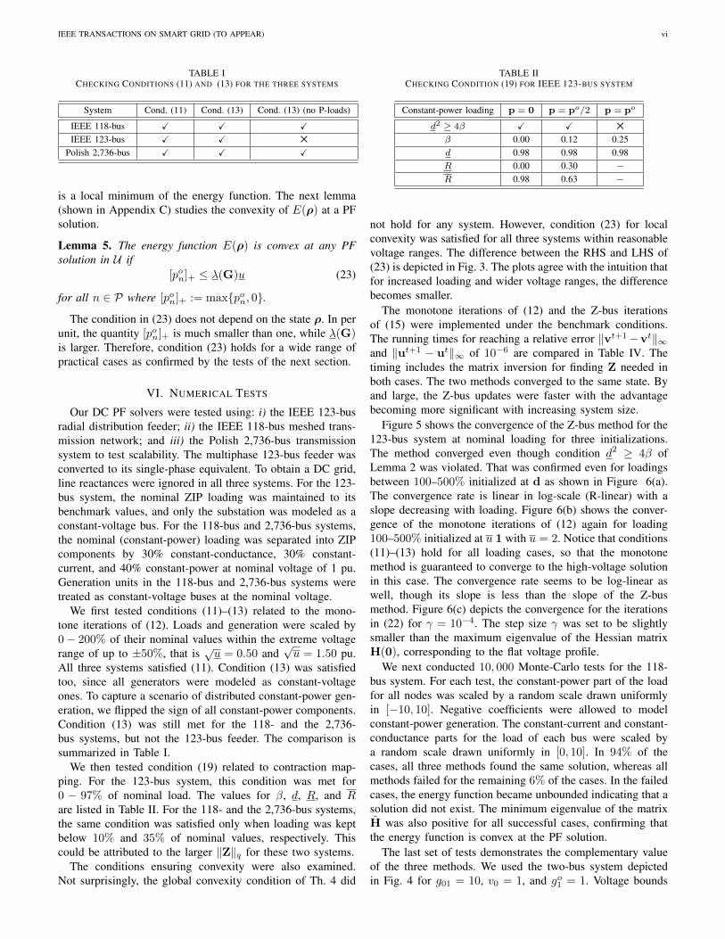
TABLE ICHECKING CONDITIONS (11) AND (13) FOR THE THREE SYSTEMS

System Cond. (11) Cond. (13) Cond. (13) (no P-loads)

IEEE 118-bus X X X

IEEE 123-bus X X 5

Polish 2,736-bus X X X

is a local minimum of the energy function. The next lemma(shown in Appendix C) studies the convexity of E(ρ) at a PFsolution.

Lemma 5. The energy function E(ρ) is convex at any PFsolution in U if

[pon]+ ≤ λ(G)u (23)

for all n ∈ P where [pon]+ := max{pon, 0}.

The condition in (23) does not depend on the state ρ. In perunit, the quantity [pon]+ is much smaller than one, while λ(G)is larger. Therefore, condition (23) holds for a wide range ofpractical cases as confirmed by the tests of the next section.

VI. NUMERICAL TESTS

Our DC PF solvers were tested using: i) the IEEE 123-busradial distribution feeder; ii) the IEEE 118-bus meshed trans-mission network; and iii) the Polish 2,736-bus transmissionsystem to test scalability. The multiphase 123-bus feeder wasconverted to its single-phase equivalent. To obtain a DC grid,line reactances were ignored in all three systems. For the 123-bus system, the nominal ZIP loading was maintained to itsbenchmark values, and only the substation was modeled as aconstant-voltage bus. For the 118-bus and 2,736-bus systems,the nominal (constant-power) loading was separated into ZIPcomponents by 30% constant-conductance, 30% constant-current, and 40% constant-power at nominal voltage of 1 pu.Generation units in the 118-bus and 2,736-bus systems weretreated as constant-voltage buses at the nominal voltage.

We first tested conditions (11)–(13) related to the mono-tone iterations of (12). Loads and generation were scaled by0− 200% of their nominal values within the extreme voltagerange of up to ±50%, that is

√u = 0.50 and

√u = 1.50 pu.

All three systems satisfied (11). Condition (13) was satisfiedtoo, since all generators were modeled as constant-voltageones. To capture a scenario of distributed constant-power gen-eration, we flipped the sign of all constant-power components.Condition (13) was still met for the 118- and the 2,736-bus systems, but not the 123-bus feeder. The comparison issummarized in Table I.

We then tested condition (19) related to contraction map-ping. For the 123-bus system, this condition was met for0 − 97% of nominal load. The values for β, d, R, and Rare listed in Table II. For the 118- and the 2,736-bus systems,the same condition was satisfied only when loading was keptbelow 10% and 35% of nominal values, respectively. Thiscould be attributed to the larger ‖Z‖q for these two systems.

The conditions ensuring convexity were also examined.Not surprisingly, the global convexity condition of Th. 4 did

TABLE IICHECKING CONDITION (19) FOR IEEE 123-BUS SYSTEM

Constant-power loading p = 0 p = po/2 p = po

d2 ≥ 4β X X 5

β 0.00 0.12 0.25d 0.98 0.98 0.98R 0.00 0.30 −R 0.98 0.63 −

not hold for any system. However, condition (23) for localconvexity was satisfied for all three systems within reasonablevoltage ranges. The difference between the RHS and LHS of(23) is depicted in Fig. 3. The plots agree with the intuition thatfor increased loading and wider voltage ranges, the differencebecomes smaller.

The monotone iterations of (12) and the Z-bus iterationsof (15) were implemented under the benchmark conditions.The running times for reaching a relative error ‖vt+1−vt‖∞and ‖ut+1 − ut‖∞ of 10−6 are compared in Table IV. Thetiming includes the matrix inversion for finding Z needed inboth cases. The two methods converged to the same state. Byand large, the Z-bus updates were faster with the advantagebecoming more significant with increasing system size.

Figure 5 shows the convergence of the Z-bus method for the123-bus system at nominal loading for three initializations.The method converged even though condition d2 ≥ 4β ofLemma 2 was violated. That was confirmed even for loadingsbetween 100–500% initialized at d as shown in Figure 6(a).The convergence rate is linear in log-scale (R-linear) with aslope decreasing with loading. Figure 6(b) shows the conver-gence of the monotone iterations of (12) again for loading100–500% initialized at u 1 with u = 2. Notice that conditions(11)–(13) hold for all loading cases, so that the monotonemethod is guaranteed to converge to the high-voltage solutionin this case. The convergence rate seems to be log-linear aswell, though its slope is less than the slope of the Z-busmethod. Figure 6(c) depicts the convergence for the iterationsin (22) for γ = 10−4. The step size γ was set to be slightlysmaller than the maximum eigenvalue of the Hessian matrixH(0), corresponding to the flat voltage profile.

We next conducted 10, 000 Monte-Carlo tests for the 118-bus system. For each test, the constant-power part of the loadfor all nodes was scaled by a random scale drawn uniformlyin [−10, 10]. Negative coefficients were allowed to modelconstant-power generation. The constant-current and constant-conductance parts for the load of each bus were scaled bya random scale drawn uniformly in [0, 10]. In 94% of thecases, all three methods found the same solution, whereas allmethods failed for the remaining 6% of the cases. In the failedcases, the energy function became unbounded indicating that asolution did not exist. The minimum eigenvalue of the matrixH was also positive for all successful cases, confirming thatthe energy function is convex at the PF solution.

The last set of tests demonstrates the complementary valueof the three methods. We used the two-bus system depictedin Fig. 4 for g01 = 10, v0 = 1, and go1 = 1. Voltage bounds

IEEE TRANSACTIONS ON SMART GRID (TO APPEAR) vii

1 50 100 150 2001

50

100

150

200

-3

-2

-1

0

1

2

(a) IEEE 123-bus system

1 50 100 150 2001

50

100

150

200

-3

-2

-1

0

1

2

(b) IEEE 118-bus system

1 50 100 150 2001

50

100

150

200

-3

-2

-1

0

1

2

(c) Polish 2,736-bus system

Fig. 3. The difference between the RHS and LHS of (23) over the voltage range defined as√u − √u in pu: Positive values mean the energy function is

convex (system stability) at all PF solutions within U .

Fig. 4. Two-bus example system.

1 2 3 4 5

Iteration number

10-10

10-5

100

‖vt−

v(t−1)‖∞

d1(d+R)1

(d+R)1

Fig. 5. Convergence of (15) for different initializations.

were set as√u = 0.9 and

√u = 1.1. The two solutions for

voltage v1 can be found in closed form. A summary of theparameters and results of the four cases considered is providedin Table III. For cases a) and b), all three methods successfullyfound the solution. Although condition (19) was not satisfiedunder scenario b), the contraction mapping found the solution.Under case c), the contraction mapping failed, while the othertwo methods found the solution. Under case d), the contractionmapping and the monotone mapping failed, but the energyfunction-based method was successful. Having cases wherethe conditions fail and the algorithm fails too demonstratesthat the conditions are not inconsequential for the practicalsuccess of the algorithm. This was true for both monotoneand contraction mappings.

VII. CONCLUSIONS

We have considered the DC PF task for possibly meshednetworks hosting ZIP loads; (large) constant-voltage gener-ators; and (smaller) constant-power generators. Under smallconstant-power generation, the suggested monotone mappingfinds the high-voltage PF solution. Under limited constant-power generation and demand, the Z-bus iterations convergeto a PF solution. The latter solution is known to exist andbe unique within a predefined ball. For reasonably limitedconstant-power demand, the energy function minimizationperspective has established that all PF solutions are localminima of the energy function. Interestingly, the first methodoperates on the space of squared voltages; the second onvoltages; and the third on the logarithm of voltages. Numericaltests have demonstrated that the iterates converge to the samePF solution even when the conditions fail. Nevertheless, theanalysis attributes different critical features to this solution.For a few hundreds of buses, the monotone mapping and theZ-bus iterates seem to be comparable in terms of executiontime. Yet for networks having thousands of buses, the latterhas an indisputable advantage.

APPENDIX AProof of Theorem 1: Mapping f(u) is monotone in U if

and only if

f(u + αen) ≥ f(u), ∀ n ∈ P (24)

for all α ≥ 0 such that u + αen ∈ U , and en is the n-thcolumn of the identity matrix of size P .

Consider the condition in (24) for a particular n ∈ P . Sinceall but the n-th entries remain unchanged between u + αenand u, it is not hard to see that

fm(u + αen)− fm(u)

=gmncm

[√um(un + α)−

√umun

]≥ 0 ∀m 6= n.

Hence, the mapping f(u) is monotone in U if and only iffn(u + αen) ≥ fn(u) for all n ∈ P . From the definition offn(u), it follows that

fn(u + αen)− fn(u)

=∑m∈P

gnmcn

(√(un + α)um −

√unum

)

IEEE TRANSACTIONS ON SMART GRID (TO APPEAR) viii

TABLE IIICHECKING CONDITIONS AND SUCCESS FOR EACH METHOD FOR THE SYSTEM OF FIG. 4

Case (19) (11)/(13) Contraction mapping Monotone mapping Energy function approacha) po = −1, io = 1 X X X X X

b) po = −2, io = 1 5 X X X X

c) po = −2, io = 10 5 5 X 5 X

d) po = −5, io = 20 5 5 5 5 X

1 2 3 4 5 6 7 8 9 101110

-8

10-6

10-4

10-2

100

100%

200%

300%

400%

500%

(a)

1 5000 10000 1500010

-8

10-6

10-4

10-2

100

100%

200%

300%

400%

500%

(b)

1 100000 20000010

-8

10-6

10-4

10-2

100

100%

200%

300%

400%

500%

(c)

Fig. 6. Convergence of (15) in (a); of (9) in (b); and (22) in (c), for different loading conditions of the IEEE 123-bus system.

TABLE IVRUNNING TIME [SEC]

System Monotone updates (12) Z-bus updates (15)

IEEE 118-bus 0.283 0.007IEEE 123-bus 0.593 0.007

Polish 2,736-bus 1,111.53 1.223

+kncn

(√un + α−

√un). (25)

Since the square root is a concave function, the differences√(un + α)um −

√unum for m ∈ P \ {n} appearing in the

RHS of (25) can be lower bounded as√(un + α)um −

√unum ≥

α

2

√um

un + α≥ α

2

√u

2u− u

since u− u ≥ α to ensure u + αen ∈ U . Therefore, the firstsummand in the RHS of (25) is positive for all n ∈ P .

Focus next on the second term in the RHS of (25). If kn <0 or equivalently ion >

∑m∈V gnmvm, the concavity of the

square root provides the lower bound

kncn

(√un + α−

√un)≥ αkn

2cn

1√un≥ αkn

2cn

1√u.

Plugging the two previous bounds into (25) and because gmnand cn are positive by definition, it follows that

fn(u + αen)− fn(u)

≥ α

2cn

(√u

2u− u∑m∈P

gnm +kn√u

). (26)

Since α and cn are positive, the monotonicity of f(u) isensured if the quantity in the parentheses of (26) is non-

negative. Plugging the definition of kn from (6), the quantityin the parentheses becomes√

u

2u− u∑m∈P

gnm +∑m∈V

gnmvm√u− ion√

u

≥√

u

2u− u∑m∈P

gnm +∑m∈V

gnm −ion√u

≥√

u

2u− ugn −

ion√u

(27)

where the first inequality follows because vm ≥√u, and the

second inequality stems from u > u and the definition of gnin (3). The condition in (11) guarantees that the RHS of (27)is non-negative for all n ∈ P with negative kn.

If kn ≥ 0, then kncn

(√un + α−√un

)≥ 0 holds trivially,

and fn(u + αen) ≥ fn(u) from (25). For this reason, busesin P with kn ≥ 0 do not appear in the conditions of Th. 1.

Proof of Theorem 2: From Theorem 1, the condition in(11) guarantees f is monotone in U . Let us ∈ U be a PFsolution so f(us) = us. We next show that f(u) ≤ u under(13). By the definitions of cn > 0 in (6a) and fn in (9):

cnu− cnfn(u)

= u

(cn −

∑m∈P

gnm

)−√u kn + pon

= u

(gon +

∑m∈V

gnm

)−√u kn + pon

≥ u

(gon +

∑m∈V

gnm

)− u

∑m∈V

gnm +√u ion + pon

= u gon +√u ion + pon

for all n ∈ P . If the last quantity is non-negative for all n,then f(u) ≤ u follows.

IEEE TRANSACTIONS ON SMART GRID (TO APPEAR) ix

The latter shows that f maps [us, u] to [us, f(u)] ⊆ [us, u].Invoking Lemma 1 with a = us and b = u yields that theiterations in (12) initialized at u converge to a PF solution uhvsatisfying uhv ≥ u for all u ∈ [us, u]. Hence, the equilibriumuhv is in fact the high-voltage power flow solution.

APPENDIX B

Proof of Theorem 3: For the subsequent analysis, a lowerbound on voltages is needed. Since ‖v − d‖q ≤ R for allv ∈ C, it follows that ‖v − d‖∞ ≤ R or |vn − dn| ≤ Rfor all n ∈ P . Combining the latter with the reverse triangleinequality yields

vn ≥ |dn| −R, ∀n ∈ P. (28)

Under (C2), the RHS of (28) is positive, and thus, a non-trivialbound on voltages has been obtained.

For h(v) to satisfy the self-mapping property, we need toshow that ‖h(v) − d‖q ≤ R holds for all v ∈ C. Using thesub-multiplicative property of norms

‖h(v)−d‖q = ‖ZD(v)p‖q ≤ ‖Z‖q · ‖D(v)‖q · ‖p‖q. (29)

For a diagonal matrix ‖dg(x)‖q = maxn |xn| for all q ≥ 1(see e.g., [26, Th 5.6.37]). Then, from (28) we get

‖D(v)‖q =(

minn|vn|

)−1≤ (d−R)

−1.

Plugging the latter into (29) renders condition (C2) sufficientfor ensuring h(v) ∈ C.

Let us now upper bound the mapping distance:

‖h(v)− h(v)‖q = ‖ZD(v)p− ZD(v)p‖q≤ ‖Z‖q‖p‖q · ‖D(v)−D(v)‖q

≤ ‖Z‖q‖p‖q ·maxn

{∣∣∣∣ vn − vnvnvn

∣∣∣∣}≤ ‖Z‖q‖p‖q

(d−R)2·max

n|vn − vn|

=‖Z‖q‖p‖q(d−R)2

· ‖v − v‖∞

≤ ‖Z‖q‖p‖q(d−R)2

· ‖v − v‖q

where the third inequality comes from (28). Given the lastbound, condition (C3) guarantees that the contraction propertyholds for α = ‖Z‖q‖p‖q/(d−R)2.

Proof of Lemma 2: From (C2), the radius R shouldsatisfy R2 − dR + β ≤ 0. To get a non-empty feasible rangefor R, the previous convex quadratic should have a positivediscriminant, i.e., d2 ≥ 4β. Then R lies in the range betweenthe roots of the quadratic as

R ∈

[d−

√d2 − 4β

2,d+

√d2 − 4β

2

]. (30)

Condition (C3) yields that |d−R| >√β. Because of (C1),

the latter simplifies as R < d−√β, thus tightening (C1) as

R ∈[0, d−

√β]. (31)

The radius R should satisfy both (30) and (31). For thelower side, it is not hard to see that because β ≥ 0

d−√d2 − 4β

2≥ 0.

For the upper side and since d ≥ 2√β, one can write

d2 − 4β =(d− 2

√β)(

d+ 2√β)≥ (d− 2

√β)2. (32)

From (32), it follows that

d+√d2 − 4β

2≥d+

(d− 2

√β)

2= d−

√β.

Combining the two sides yields the range of (18). Using (32)and because d2 ≥ 4β, we obtain that

d−√d2 − 4β

2≤d−

(d− 2

√β)

2≤√β ≤ d−

√β

so that the range of this lemma is not empty.Proof of Lemma 3: Similar to the proof of Theorem 3,

if v ∈ CR, then |vn − dn| ≤ R for all n ∈ P . Combining thelatter and the reverse triangular inequality yields,

|dn| −R ≤ |vn| ≤ |dn|+R.

A sufficient condition for vn ∈ [√u,√u] is that

√u ≤ |dn|−R

and |dn|+R ≤√u. These two inequalities will hold if R ≤

min{d−√u,

√u− d

}, which concludes the proof.

Proof of Lemma 4: The set V is contained in CR if allof its corners belong to CR. In other words, if vc is a corner(extreme) point of V , it should hold that ‖vc−d‖q ≤ R. Thetriangle inequality yields

‖vc − d‖q ≤∥∥∥vc − (√u+√u2

)1∥∥∥q

+∥∥∥(√u+√u2

)1− d

∥∥∥q

where(√

u+√u

2

)1 is the center point of the hypercube V .

Since all corner points of V have the same distance to thiscenter points, the point vc can be selected as

√u1 without

loss of generality, for which it holds that∥∥∥∥∥vc −(√

u+√u

2

)1

∥∥∥∥∥q

=

(√u−√u

2

)‖1‖q.

Plugging the latter into the upper bound for ‖vc−d‖q provesthe claim.

APPENDIX C

Proof of Theorem 4: Decompose H(ρ) as H(ρ) = G+K(ρ), where K(ρ) is a diagonal matrix with diagonal entries

Knn(ρ) := cn − kne−ρn2 −

∑m∈P

gnmeρm−ρn

2 .

If voltages lie in U , Knn(ρ)’s can be lower bounded as

Knn(ρ) ≥ cn −[kn]+√u−√u

u

∑m∈P

gnm. (33)

The minimum eigenvalue of H satisfies [27, Th. 3.2.1]

λ(H(ρ)) ≥ λ(G) + λ(K(ρ)). (34)

IEEE TRANSACTIONS ON SMART GRID (TO APPEAR) x

Plugging (33) into (34) yields

λ(H) ≥ λ(G) + cn −[kn]+√u−√u

u

∑m∈P

gnm.

For λ(H) ≥ 0, the RHS of the last inequality must be positivefor all n ∈ P , which is ensured by the condition of thistheorem.

Proof of Lemma 5: If ρo is a PF solution, it satisfies (21)for all n ∈ P . Exploiting this fact and from the definition ofKnn(ρ), it follows that

Knn(ρo) = −pone−ρon

≥ − [pon]+u

.

Using (34) again, condition (23) ensures λ(H(ρo)) ≥ 0.

REFERENCES

[1] H. Mohsenian-Rad and A. Davoudi, “Towards building an optimaldemand response framework for DC distribution networks,” IEEE Trans.Smart Grid, vol. 5, no. 5, pp. 2626–2634, Sep. 2014.

[2] D. Salomonsson and A. Sannino, “Low-Voltage DC Distribution Systemfor Commercial Power Systems With Sensitive Electronic Loads,” IEEETrans. Power Delivery, vol. 22, no. 3, pp. 1620–1627, Jul. 2007.

[3] A. Sannino, G. Postiglione, and M. H. J. Bollen, “Feasibility of a DCnetwork for commercial facilities,” IEEE Trans. Ind. Applicat., vol. 39,no. 5, pp. 1499–1507, Sep. 2003.

[4] D. Nilsson and A. Sannino, “Efficiency analysis of low- and medium-voltage DC distribution systems,” in Proc. IEEE PES General Meeting,Denver, CO, Jun. 2004, pp. 2315–2321.

[5] H. Ergun, J. Beerten, and D. V. Hertem, “Building a new overlay gridfor Europe,” in Proc. IEEE PES General Meeting, San Diego, CA, Jul.2012.

[6] B. C. Lesieutre, P. W. Sauer, and M. A. Pai, “Existence of solutionsfor the network/load equations in power systems,” IEEE Trans. CircuitsSyst. I, vol. 46, no. 8, pp. 1003–1011, Aug. 1999.

[7] D. K. Molzahn, B. C. Lesieutre, and C. L. DeMarco, “A sufficientcondition for power flow insolvability with applications to voltagestability margins,” IEEE Trans. Power Syst., vol. 28, no. 3, pp. 2592–2601, Aug. 2013.

[8] W. Ma and J. S. Thorp, “An efficient algorithm to locate all the loadflow solutions,” IEEE Trans. Power Syst., vol. 8, no. 3, pp. 1077–1083,Aug. 1993.

[9] D. K. Molzahn, D. Mehta, and M. Niemerg, “Toward topologically-based upper bounds on the number of power flow solutions,” in Proc.American Control Conf., Boston, MA, Jul. 2016.

[10] H. D. Chiang and M. E. Baran, “On the existence and uniqueness ofload flow solution for radial distribution power networks,” IEEE Trans.Circuits Syst., vol. 37, no. 3, pp. 410–416, Mar. 1990.

[11] S. Bolognani and S. Zampieri, “On the existence and linear approxima-tion of the power flow solution in power distribution networks,” IEEETrans. Power Syst., vol. 31, no. 1, pp. 163–172, Jan. 2016.

[12] D. Mehta, D. K. Molzahn, and K. Turitsyn, “Recent advances incomputational methods for the power flow equations,” in Proc. AmericanControl Conf., Boston, MA, Jul. 2016, pp. 1753–1765.

[13] J. W. Simpson-Porco, F. Dorfler, and F. Bullo, “On resistive networksof constant-power devices,” IEEE Trans. Circuits Syst. II, vol. 62, no. 8,pp. 811–815, Aug. 2015.

[14] J. W. Simpson-Porco, “A Theory of Solvability for Lossless Power FlowEquations-Part II: Fixed-Point Power Flow,” IEEE Trans. Control ofNetwork Systems, vol. 5, no. 3, pp. 1361–1372, Sep. 2018.

[15] ——, “A Theory of Solvability for Lossless Power Flow Equations-PartII: Conditions for Radial Networks,” IEEE Trans. Control of NetworkSystems, vol. 5, no. 3, pp. 1373–1385, Sep. 2018.

[16] M. Bazrafshan and N. Gatsis, “Convergence of the Z-bus method forthree-phase distribution load-flow with ZIP loads,” IEEE Trans. PowerSyst., vol. 33, no. 1, pp. 153–165, Jan. 2018.

[17] ——, “Convergence of the Z-bus method and existence of uniquesolution in single-phase distribution load-flow,” in Proc. IEEE GlobalConf. on Signal and Information Process., Washington, DC, Dec. 2016.

[18] A. Garces, “Uniqueness of the power flow solutions in low voltage directcurrent grids,” Electric Power Systems Research, vol. 151, pp. 149–153,Oct. 2017.

[19] K. Dvijotham, E. Mallada, and J. W. Simpson-Porco, “High-voltagesolution in radial power networks: Existence, properties, and equivalentalgorithms,” IEEE Control Systems Lett., vol. 1, no. 2, pp. 322–327, Oct.2017.

[20] L. Gan and S. H. Low, “Optimal power flow in direct current networks,”IEEE Trans. Power Syst., vol. 29, no. 6, pp. 2892–2904, Nov. 2014.

[21] K. Dvijotham, S. Low, and M. Chertkov, “Convexity of energy-like functions: Theoretical results and applications to power systemoperations,” 2015. [Online]. Available: https://arxiv.org/abs/1501.04052

[22] T. Dragicevic, X. Lu, J. C. Vasquez, and J. M. Guerrero, “DC microgrids– Part I: A review of control strategies and stabilization techniques,”IEEE Trans. Power Electron., vol. 31, no. 7, pp. 4876–4891, Jul. 2016.

[23] M. Angjelichinoski, A. Scaglione, P. Popovski, and C. Stefanovic,“Decentralized DC microgrid monitoring and optimization via primarycontrol perturbations,” vol. 66, no. 12, pp. 3280–3295, Dec. 2018.

[24] C. Godsil and G. Royle, Algebraic Graph Theory. New York, NY:Springer, 2001.

[25] W. A. Kirk and B. Sims, Eds., Handbook of Metric Fixed Point Theory.Springer, Dordrecht, 2001.

[26] R. A. Horn and C. R. Johnson, Eds., Matrix Analysis. Cambridge, UK:Cambridge University Press, 1986.

[27] R. Bhatia, Matrix Analysis. Springer, vol. 169.

Sina Taheri received the B.S. degree from SharifUniversity of Technology, Tehran, Iran, in 2016; andthe M.Sc. degree from Virginia Tech, Blacksburg,VA, USA, in 2019; both in electrical engineering.He is currently pursuing a Ph.D. degree at VirginiaTech. His research interests are focused on theapplication of optimization, machine learning, andgraph-theoretic techniques to develop algorithmicsolutions for monitoring and operation of smartpower systems.

Vassilis Kekatos (SM’16) is an Assistant Professorwith the Bradley Dept. of ECE at Virginia Tech. Heobtained his Diploma, M.Sc., and Ph.D. from theUniv. of Patras, Greece, in 2001, 2003, and 2007,respectively. He is a recipient of the NSF CareerAward in 2018 and the Marie Curie Fellowship. Hehas been a research associate with the ECE Dept.at the Univ. of Minnesota, where he received thepostdoctoral career development award (honorablemention). During 2014, he stayed with the Univ. ofTexas at Austin and the Ohio State Univ. as a visiting

researcher. His research focus is on optimization and learning for future energysystems. He is currently serving in the editorial board of the IEEE Trans. onSmart Grid.