ieee transactions on visualization & computer graphics...

IEEE TRANSACTIONS ON VISUALIZATION & COMPUTER GRAPHICS 1

Coloring 3D Printed Surfaces by ThermoformingYizhong Zhang, Student Member, IEEE, Yiying Tong, Member, IEEE, and Kun Zhou, Fellow, IEEE

Abstract—Decorating the surfaces of 3D printed objects with color textures is still not readily available in most consumer-level or evenhigh-end 3D printers. Existing techniques such as hydrographics color transfer suffer from the issues of air pockets in concave regionsand discoloration in overly stretched regions. We propose a novel thermoforming-based coloring technique to alleviate these problemsas well as to simplify the overall procedure. Thermoforming is a widely used technique in industry for plastic thin shell productmanufacturing by pressing heated plastic sheets onto molds using atmospheric pressure. We attach on the transparent plastic sheet aprecomputed color pattern decal prior to heating, and adhere it to 3D printed models treated as the molds in thermoforming. The 3Dmodels are thus decorated with the desired color texture, as well as a thin, polished protective cover. The precomputation involves aphysical simulation of the thermoforming process to compute the correct color pattern on the plastic sheet, and the vent hole layout onthe 3D model for air pocket elimination. We demonstrate the effectiveness and accuracy of our computational model and our prototypethermoforming surface coloring system through physical experiments.

Index Terms—3D printing, thermoforming, thermoplastic sheet simulation, texture mapping

F

1 INTRODUCTION

THe past few years have witnessed a rapid increase inthe popularity of 3D printing, e.g., for fast prototyping.

However, coloring the surface of the printed model remainschallenging, especially for concave regions. While high-end 3D printers do provide the possibility of printing the3D model with colored surface, most of them use limitedmaterials, and are slow and costly to produce the desired ap-pearance. The state-of-the-art computational hydrographicprinting allows the decoration of the surface after the 3Dprinting is done (e.g., [1], [2]). However, such methods stillhave difficulties in covering highly concave regions.

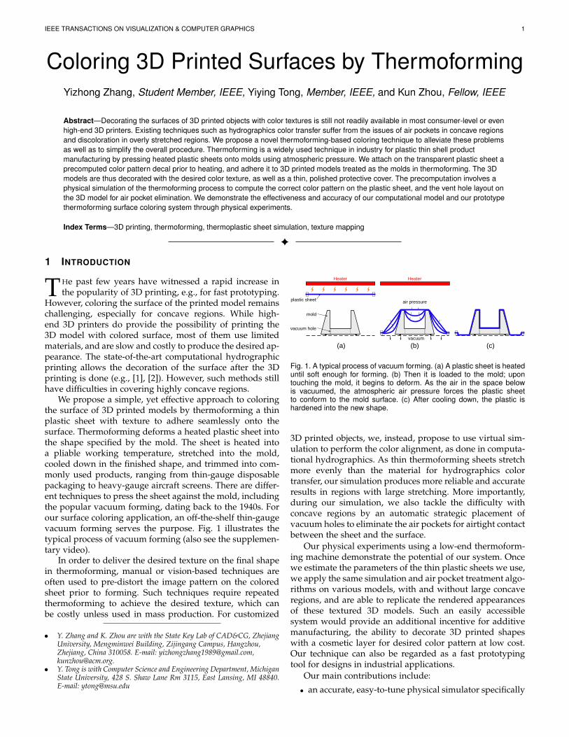
We propose a simple, yet effective approach to coloringthe surface of 3D printed models by thermoforming a thinplastic sheet with texture to adhere seamlessly onto thesurface. Thermoforming deforms a heated plastic sheet intothe shape specified by the mold. The sheet is heated intoa pliable working temperature, stretched into the mold,cooled down in the finished shape, and trimmed into com-monly used products, ranging from thin-gauge disposablepackaging to heavy-gauge aircraft screens. There are differ-ent techniques to press the sheet against the mold, includingthe popular vacuum forming, dating back to the 1940s. Forour surface coloring application, an off-the-shelf thin-gaugevacuum forming serves the purpose. Fig. 1 illustrates thetypical process of vacuum forming (also see the supplemen-tary video).

In order to deliver the desired texture on the final shapein thermoforming, manual or vision-based techniques areoften used to pre-distort the image pattern on the coloredsheet prior to forming. Such techniques require repeatedthermoforming to achieve the desired texture, which canbe costly unless used in mass production. For customized

• Y. Zhang and K. Zhou are with the State Key Lab of CAD&CG, ZhejiangUniversity, Mengminwei Building, Zijingang Campus, Hangzhou,Zhejiang, China 310058. E-mail: [email protected],[email protected].

• Y. Tong is with Computer Science and Engineering Department, MichiganState University, 428 S. Shaw Lane Rm 3115, East Lansing, MI 48840.E-mail: [email protected]

Heater Heater

air pressureplastic sheet

mold

vacuum hole

vacuum

(a) (b) (c)

Fig. 1. A typical process of vacuum forming. (a) A plastic sheet is heateduntil soft enough for forming. (b) Then it is loaded to the mold; upontouching the mold, it begins to deform. As the air in the space belowis vacuumed, the atmospheric air pressure forces the plastic sheetto conform to the mold surface. (c) After cooling down, the plastic ishardened into the new shape.

3D printed objects, we, instead, propose to use virtual sim-ulation to perform the color alignment, as done in computa-tional hydrographics. As thin thermoforming sheets stretchmore evenly than the material for hydrographics colortransfer, our simulation produces more reliable and accurateresults in regions with large stretching. More importantly,during our simulation, we also tackle the difficulty withconcave regions by an automatic strategic placement ofvacuum holes to eliminate the air pockets for airtight contactbetween the sheet and the surface.

Our physical experiments using a low-end thermoform-ing machine demonstrate the potential of our system. Oncewe estimate the parameters of the thin plastic sheets we use,we apply the same simulation and air pocket treatment algo-rithms on various models, with and without large concaveregions, and are able to replicate the rendered appearancesof these textured 3D models. Such an easily accessiblesystem would provide an additional incentive for additivemanufacturing, the ability to decorate 3D printed shapeswith a cosmetic layer for desired color pattern at low cost.Our technique can also be regarded as a fast prototypingtool for designs in industrial applications.

Our main contributions include:

• an accurate, easy-to-tune physical simulator specifically


designed for thermoforming,• an automatic vacuum hole placement algorithm based

on the topological changes of air pockets during thedeformation,

• and an end-to-end prototype system from the pre-warping of texture based on physical simulation, print-ing of colored sheet, 3D printing of the vented model,to thermoforming of the sheet onto the 3D model.

2 RELATED WORK

3D Printing. As additive manufacturing, or 3D printingtechnology matured, there has been a surge of methodsfor customizing the desired physical properties of the solidvolume (e.g., [3], [4], [5], [6], [7], [8], [9], [10], [11], [12], [13].Techniques have also been proposed to develop a thin layerof material with desired reflectance properties by mixingheterogeneous materials, surpassing the regular RGB colorprinting (e.g., [14], [15], [16], [17], [18], [19]. However, thesemethods do not provide insights on affordable full-colorprinting of a textured 3D model.Surface Coloring. While it is possible to directly print thetextured 3D models with high-end 3D printers, or withadditional techniques such plating or enameling [20], [21],such procedures are not only costly but also with limita-tions on the target model material or choices on colors.Vinyl decals [22] and hydrographics provide techniques thatare hard to control the precise locations of the pixels oncurved surfaces. The most successful affordable approachesso far include computational hydrographic printing [1] andtexture mapping real-world objects with hydrographics [2].Both transfer pigments printed on a flat sheet onto curvedsurfaces with a technique called hydrographics, both mini-mize the distortion of the desired appearance through pre-warping of the texture based on simulated deformation ofthe sheet as it is attached to the surface, and both suffer fromthe air pockets formed during the transfer onto concaveregions. Our method is designed to tackle the problem ofair pockets in these regions while offering a simpler and“dry” overall procedure.Thermoforming. We address the issue of air pockets byresorting to a different technique, thermoforming, which,by design, exhaust air from the space between the colorsheet and the surface. As thermoforming has been a matureplastic fabrication technique widely used in industry fordecades (see, e.g., the textbook on thermoforming [23]), weonly review the most related methods. Using 3D printing asrapid tooling for thermoforming molds has been proposedin, e.g., [24]. However, the method does not address theissue of surface coloring, and it requires human interven-tion in designing the whole mold, including the layout ofvacuum holes.

There are also existing methods for image pre-distortionbased on computer vision (e.g., [25], [26]). However, suchmethods would have to physically perform the thermoform-ing for individual shapes. For large customized models, theprototyping can be costly and slow, with results at the mercyof the accuracy of vision registration methods and the inkused. Most inks would change intensity under distortionin thermoforming [27]. In contrast, our method does notrequire a physical experiment with each shape. Once the

parameters of a type of thin sheet and a thermoformingmachine are determined, it can be used to decorate anyshapes, as long as they fit into the effective regions of themachine. We can also pre-adjust the ink intensity as wedemonstrate later, which is impossible prior to a virtualsimulation.

Concurrent to our work, Schuller et al. [28] also intro-duced a method of producing colored 3D models by ther-moforming. These two methods use the viscous thin-sheetmodel with linear elasticity in the membrane energy withadded plasticity. The main differences are that their methodincludes bending energy and ours includes adhesion forcecalculation before vacuuming, but the simulation resultsare similar. Our method contains additionally an automaticvacuum hole layout algorithm, enabling proper handling ofhighly concave regions.Virtual Simulation of Thermoforming. Commercial soft-ware T-Sim developed by Accuform Corporation [29] isdesigned to simulate the process of thermoforming, sothat the usability of the mold can be evaluated beforefabricated. While it provides various additional tools forthermoforming, such as plug assists, its treatment on imagepre-distortion to provide better image alignment is severelylimited. It lacks the capability of locating or even addingvacuum holes in the mold to reduce air pockets, providesno color adjustment technique to reduce color deviationdue to stretch, and only takes a top view image insteadof a texture atlas as input. We implement our simulationof heated plastic thin sheet under air pressure based onfinite element methods, as done in [30], [31], [32]. Theheated plastic sheet behaves both elastically and plastically,so viscous sheet simulations are inadequate. Following [33],we use hyperelastic material properties as the basis of oursimulation of the sheet. Multiplicative volume-preservingplasticity has been used in volumetric simulation such as[34], [35] and in thin sheet simulation [36]. We adapt themultiplicative plasticity model to be area-preserving witha simplified simulation as bending can be ignored withthe fixed boundary condition in vacuum forming [30] andneither fracture nor tearing is present in the process. Wefurther introduced a topological change tracking during thesimulation, for the automatic vent hole layout determinationbased on concepts from computational topology [37].

3 OVERVIEW

The general idea of our method is to simulate the thermo-forming process on the given textured shape before creatingthe physical model. The purpose of the simulation is to pre-distort the texture and locate the vent holes on the 3D model.

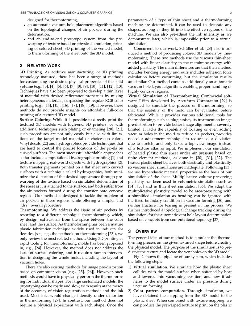
Fig. 2 shows the pipeline of our system, which includesthe following steps:1) Virtual simulation. We simulate how the plastic sheet

collides with the model surface when softened by heatand lowered into vacuuming position, and how it ad-heres to the model surface under air pressure duringvacuum forming.

2) Color pattern computation. Through simulation, wehave obtained the mapping from the 3D model to theplastic sheet. When combined with texture mapping, wecan produce the prewarped texture to print on the plastic


Input: textured 3D model Simulation Vented 3D model

Pattern to print

OutputVacuum formingPrinted model

Printed sheet

Fig. 2. The pipeline of our system. Our system takes a textured 3D digital model as input. By simulating the thermoforming process virtually, wecan compute the correspondence map between the plastic sheet and the model surface, which will be used to calculate the pattern to print on thesheet. By tracking the motion of the plastic sheet, potential air pockets can be detected, which will be resolved by setting vacuum holes on the 3Dmodel. Finally, the actual vacuum forming is performed using the plastic sheet with the printed color pattern and the 3D printed vented model on avacuum forming machine. The final product is a 3D model decorated with the desired color texture.

sheet to achieve desired appearance after thermoform-ing.

3) Vacuum hole placement. In the vacuuming process,air pockets may form in concave regions of the mold,preventing the plastic sheet from adhering tightly to thesurface. Based on the simulation, we detect potential airpockets by tracking topological changes of the cavitiesformed between the plastic sheet and the model, andthen refine the 3D model by populating internal vacuumholes in optimal locations to eliminate the air pockets.

4) Vacuum forming. Finally, we carry out the physicalprocess of thermoforming the color printed sheet ontothe 3D printed model.

4 SIMULATION OF THERMOFORMING

The main purpose of our thermoforming simulation is todetermine the color pattern to print on the plastic sheet, sothat the desired appearance will be attached to the surfaceof the 3D model. Thus, the key result is the correspondencesbetween each pixel on the sheet and the surface point that itattaches to by the end of the simulation.

4.1 Thermoplastic Sheet

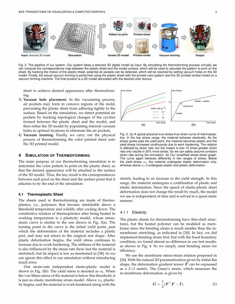
The sheets used in thermoforming are made of thermo-plastics, i.e., polymers that become stretchable above athreshold temperature and solidify after cooling down. Theconstitutive relation of thermoplastics after being heated toworking temperature is a plasticity model, whose stress-strain curve is similar to the one shown in Fig. 3(a). Theturning point in the curve is the initial yield point, pastwhich the deformation of the material includes a plasticpart, and may not return to the original rest shape. Afterplastic deformation begins, the yield stress continues toincrease due to work hardening. The stiffness of the materialis also influenced by the strain rate (how fast the material isstretched), but its impact is low as mentioned in [38]. So wecan ignore this effect in our simulation without introducingmuch error.

Our strain-rate independent elasto-plastic model isshown in Fig. 3(b). The yield stress is denoted as σ0. Whenthe von Mises stress of the material is below this threshold, itis just an elastic membrane strain model. Above σ0, plastic-ity begins, and the material is work-hardened along with the

true strain

true stress

strain rate (s-1)

0.11

10

(a)true strain

true stress

(b)

σ0

elastic

elastic + plastic

yield point

Fig. 3. (a) A typical physical true stress-true strain curve of thermoplas-tics. In the low stress range, the material behaves elastically. As thestress grows past the yield point, the material becomes plastic and theyield stress increases continuously due to work hardening. The relationis affected by strain rate, but the impact is low–10 times greater strainrate only results in 20% more stress. So we can safely assume constantstrain rate during the simulation. (b) Our simplified stress-strain graph.The curve again behaves differently in two ranges of stress. Belowthe yield stress σ0, the material undergoes elastic deformation only,whereas above σ0 it undergoes elastic and plastic deformation.

stretch, leading to an increase in the yield strength. In thisrange, the material undergoes a combination of plastic andelastic deformation. Since the speed of elastic-plastic sheetdeformation does not change the result by much, the modelwe use is independent of time and is solved in a quasi-staticmanner.

4.1.1 Elasticity.

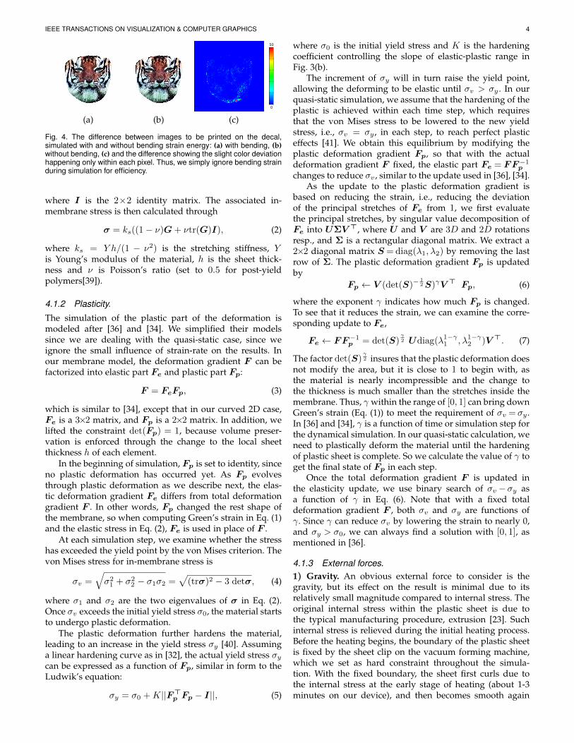
The plastic sheets for thermoforming have thin-shell struc-tures, but the heated polymer can be modeled as mem-brane since the bending strain is much smaller than the in-membrane stretching, as indicated in [30]. In fact, we didimplement bending strain first, but with the fixed boundarycondition, we found almost no difference in our test results,as shown in Fig. 4. So we simply omit bending strain forefficiency.

We use the membrane stress-strain relation proposed in[36]. With the natural 2D parametrization given by initial flatshape, the deformation gradient tensor F can be expressedas a 3×2 matrix. The Green’s strain, which measures thein-membrane deformation, is given by

G =1

2(F>F − I), (1)


50

0

(a) (b) (c)

Fig. 4. The difference between images to be printed on the decal,simulated with and without bending strain energy: (a) with bending, (b)without bending, (c) and the difference showing the slight color deviationhappening only within each pixel. Thus, we simply ignore bending strainduring simulation for efficiency.

where I is the 2×2 identity matrix. The associated in-membrane stress is then calculated through

σ = ks((1− ν)G+ νtr(G)I), (2)

where ks = Y h/(1 − ν2) is the stretching stiffness, Yis Young’s modulus of the material, h is the sheet thick-ness and ν is Poisson’s ratio (set to 0.5 for post-yieldpolymers[39]).

4.1.2 Plasticity.

The simulation of the plastic part of the deformation ismodeled after [36] and [34]. We simplified their modelssince we are dealing with the quasi-static case, since weignore the small influence of strain-rate on the results. Inour membrane model, the deformation gradient F can befactorized into elastic part Fe and plastic part Fp:

F = FeFp, (3)

which is similar to [34], except that in our curved 2D case,Fe is a 3×2 matrix, and Fp is a 2×2 matrix. In addition, welifted the constraint det(Fp) = 1, because volume preser-vation is enforced through the change to the local sheetthickness h of each element.

In the beginning of simulation, Fp is set to identity, sinceno plastic deformation has occurred yet. As Fp evolvesthrough plastic deformation as we describe next, the elas-tic deformation gradient Fe differs from total deformationgradient F . In other words, Fp changed the rest shape ofthe membrane, so when computing Green’s strain in Eq. (1)and the elastic stress in Eq. (2), Fe is used in place of F .

At each simulation step, we examine whether the stresshas exceeded the yield point by the von Mises criterion. Thevon Mises stress for in-membrane stress is

σv =√σ21 + σ2

2 − σ1σ2 =√(trσ)2 − 3 detσ, (4)

where σ1 and σ2 are the two eigenvalues of σ in Eq. (2).Once σv exceeds the initial yield stress σ0, the material startsto undergo plastic deformation.

The plastic deformation further hardens the material,leading to an increase in the yield stress σy [40]. Assuminga linear hardening curve as in [32], the actual yield stress σycan be expressed as a function of Fp, similar in form to theLudwik’s equation:

σy = σ0 +K||F>p Fp − I||, (5)

where σ0 is the initial yield stress and K is the hardeningcoefficient controlling the slope of elastic-plastic range inFig. 3(b).

The increment of σy will in turn raise the yield point,allowing the deforming to be elastic until σv > σy. In ourquasi-static simulation, we assume that the hardening of theplastic is achieved within each time step, which requiresthat the von Mises stress to be lowered to the new yieldstress, i.e., σv = σy , in each step, to reach perfect plasticeffects [41]. We obtain this equilibrium by modifying theplastic deformation gradient Fp, so that with the actualdeformation gradient F fixed, the elastic part Fe = FF−1p

changes to reduce σv , similar to the update used in [36], [34].As the update to the plastic deformation gradient is

based on reducing the strain, i.e., reducing the deviationof the principal stretches of Fe from 1, we first evaluatethe principal stretches, by singular value decomposition ofFe into UΣV >, where U and V are 3D and 2D rotationsresp., and Σ is a rectangular diagonal matrix. We extract a2×2 diagonal matrix S =diag(λ1, λ2) by removing the lastrow of Σ. The plastic deformation gradient Fp is updatedby

Fp ← V (det(S)−12S)γV > Fp, (6)

where the exponent γ indicates how much Fp is changed.To see that it reduces the strain, we can examine the corre-sponding update to Fe,

Fe ← FF−1p = det(S)γ2 Udiag(λ1−γ1 , λ1−γ2 )V >. (7)

The factor det(S)γ2 insures that the plastic deformation does

not modify the area, but it is close to 1 to begin with, asthe material is nearly incompressible and the change tothe thickness is much smaller than the stretches inside themembrane. Thus, γ within the range of [0, 1] can bring downGreen’s strain (Eq. (1)) to meet the requirement of σv = σy .In [36] and [34], γ is a function of time or simulation step forthe dynamical simulation. In our quasi-static calculation, weneed to plastically deform the material until the hardeningof plastic sheet is complete. So we calculate the value of γ toget the final state of Fp in each step.

Once the total deformation gradient F is updated inthe elasticity update, we use binary search of σv −σy asa function of γ in Eq. (6). Note that with a fixed totaldeformation gradient F , both σv and σy are functions ofγ. Since γ can reduce σv by lowering the strain to nearly 0,and σy > σ0, we can always find a solution with [0, 1], asmentioned in [36].

4.1.3 External forces.1) Gravity. An obvious external force to consider is thegravity, but its effect on the result is minimal due to itsrelatively small magnitude compared to internal stress. Theoriginal internal stress within the plastic sheet is due tothe typical manufacturing procedure, extrusion [23]. Suchinternal stress is relieved during the initial heating process.Before the heating begins, the boundary of the plastic sheetis fixed by the sheet clip on the vacuum forming machine,which we set as hard constraint throughout the simula-tion. With the fixed boundary, the sheet first curls due tothe internal stress at the early stage of heating (about 1-3minutes on our device), and then becomes smooth again


Fig. 5. Forces in the two stages of thermoforming. (a) Loading. The plas-tic sheet slips on the mold until the membrane force fm, repulsive forcefr and friction ff reach equilibrium. (b) Vacuuming. The membraneforce fm and air pressure force fp reaches equilibrium. Any verticestouching the mold serve as position constraints.

(around 3-5 minutes). Once the working temperature isreached, the sheet is ready for forming. Throughout theheating process, there is no visible drape in the sheet asthe gravity is negligible compared to the internal stress.When the vacuuming begins, air pressure and contact forcesbecome the dominating external forces. So we simply omitgravity throughout our simulation. For large sheets, it is alsoeasy to introduce gravity through the sheet mass densitytimes the constant gravitational acceleration.2) Collision with 3D model. After the heating stage, welower the plastic sheet until the sheet clip touches the modelcontainer. At this point, the plastic sheet may touch the3D model and slide on the surface. Since the surface isstatic throughout the simulation, we pre-compute a signeddistance field for the 3D model to perform fast collisiondetection on a regular grid (with 2mm×2mm×2mm cell-size) as in [42]. Our collision handling is modeled after [43],through repulsive forces determined by the distance to thesurface. For each vertex of the sheet mesh, we check itsdistance to the 3D model surface by a trilinear interpolationof the distance field in the grid cell. If the distance valued < h0/2, where h0 is the original plastic sheet thickness(1mm in our experiments), we activate, for that vertex, arepulsive force expressed as

fr =

{kr(

h0

2 −d)M n, d < h0/2

0, otherwise, (8)

where M is one third of the one-ring area of the vertex, nis the unit gradient of the signed distance field and kr is aconstant to control the repulsive force. We found this simplemodel adequate for achieving the desired accuracy in ourexperiments.3) Friction with model surface. Friction, the tangentialcontact force, resists to slipping of the plastic sheet on the3D model surface. We use the Coulomb’s model to evaluatethe friction ff . For each vertex of sheet, the maximumfriction magnitude is µ‖fr‖, where µ is the coefficient offriction between the contacting materials. We compare themaximum friction with the magnitude of ft, which is thetangential component of the sum of all other forces f , calcu-lated through a projection onto the plane perpendicular ton. Then the friction force (Fig. 5 (a)) ff can be calculated as

ff =

{−ft, ‖ft‖ < µ‖fr‖−µ‖fr‖‖ft‖ft, otherwise

, (9)

4) Atmosphere pressure. When the plastic sheet reachesthe equilibrium state, we start the vacuum forming. At thisstage, the air pressure forces the plastic sheet to press againstthe model surface and be attached to it firmly. We graduallyincrease the air pressure until the end of the procedure. Inthe simulation, we first calculate the air pressure force oneach triangle, and then evenly distribute the force to its threevertices. The force on each triangle is calculated by

fp = −pAn, (10)

where p is the current air pressure difference between thetop and the bottom sides of the sheet, A is the area of thetriangle and n is the unit normal of the triangle. The sum ofthe distributed fp from the one-ring of a vertex provides theair pressure force on the vertex fp (Fig. 5 (b)). We assumea constant pressure difference p for all triangles, as oftendone in vacuum-based thermoforming simulations. Thisassumption also allows us to provide an efficient treatmentof air pockets formed during the process (in Sec. 5). Assoon as the air pressure brings any part of the plastic sheetinto contact with the model surface, it will be held therefirmly. So we assume no slipping in the vacuum formingstage. It means that once we detect the distance value of avertex from the surface to satisfy d < h0/2, we constrain thevertex position to be the point where d = h0/2 along theline segment between the current position and the previousposition, by iterative search. We use the original thicknessh0 in this calculation, since the thickness change of the sheetcan be safely ignored.

4.2 Implementation of Numerical SimulationWe use finite element method to simulate the plastic sheet.In our discretization of the plastic sheet, its fixed boundaryis a rectangle that fits into the sheet clip. A triangular tes-sellation of the sheet was generated using the mesh library:Triangle [44], with a lower bound of 30◦ for interior angleand an upper bound of 2mm2 for triangle area. The simu-lation starts from hanging the plastic sheet above the model(Fig. 1 (a)). We first simulate the collision of the sheet withthe model during when loaded into the working position,and then activate the pressure difference for vacuuming(Fig. 1 (b)). Since the whole procedure is fast, we can ignorethe effects of the change in temperature.

We formulate the simulation as a backward Euler up-date. In each simulation step, we first update the vertexpositions based on balancing the forces in the quasi-stepsimulation. The internal stress is calculated based on theelastic deformation gradient FF−1

p , where F is a functionof the vertex positions, and F−1

p is the plastic deformationgradient in the previous step. The other forces, includingthe air pressure, the repulsive force, and the friction, are allfunctions of the vertex positions through their dependenceon the normal, the area, and the distance to the modelsurface. Since the gradients of all the forces can be easilyderived, we solve the nonlinear force balance equations byNewton’s method, with 50 Newton iterations per simulationstep. For each iteration, the linear system was solved by aConjugate Gradient solver.

With the updated vertex position, we perform the plasticdeformation update. We first detect the triangles satisfying


(a) (b) (c)

0

2

4

6

(d)

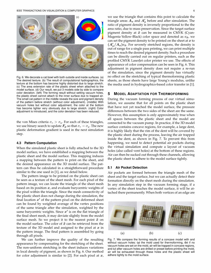
Fig. 6. We decorate a cat bowl with both outside and inside surfaces. (a)The desired texture. (b) The result of computational hydrographics, thetexture at the bottom has become highly distorted due to large stretch.(c) The area extension rate of the plastic sheet when attached to themodel surface. (d) Our result, we put 3 models side by side to comparecolor deviation. (left) The forming result without setting vacuum holes,the plastic sheet cannot attach to the inner surface due to trapped air.The small cat pattern in the middle reveals the size and pigment densityof the pattern before stretch (without color adjustment). (middle) Withvacuum holes but without color adjustment, the color at the bottomhas become lighter very obviously due to large stretch. (right) Coloradjustment is introduced, and the color deviation has been reduced.

the von Mises criteria σv > σy . For each of these triangles,we use binary search to update Fp so that σv = σy . The newplastic deformation gradient is used in the next simulationstep.

4.3 Pattern ComputationWhen the simulated plastic sheet is fully attached to the 3Dmodel surface, we have established a mapping between theplastic sheet and the model surface. This mapping inducesa mapping between the pattern to print on the sheet, andthe desired appearance on the 3D model surface. The pat-tern can thus be calculated in a straightforward proceduresimilar to the one used in [1], as we detail below.

The pattern image to be printed on the plastic sheet canbe seen as a texture of the sheet mesh. For each pixel of thepattern image, we can locate the triangle of the sheet meshbased on its position x, and evaluate barycentric weights ofthe pixel within the triangle. Since the mesh connectivity ofthe plastic sheet does not change during the simulation, thefinal location x′ of the pattern pixel on the deformed sheetcan be found by weighted average of the vertex positionsof the same triangle after the simulation, weighted by thesame barycentric weights. Since x′ is on the flat triangle ofthe final sheet mesh, it may deviate slightly from the modelsurface mesh. So we project it to the nearest point x onthe model surface. The color of x can be retrieved from thetexture of the 3D model and assigned to the pixel at x inthe pattern image. The final pattern is assembled by goingthrough all pixels.

We can further improve the quality of the resultingappearance by compensating for the stretching of the sheet.The non-uniform stretching in the sheet induces variationsin local density of pigment, as shown in Fig. 6. Our methodfor color adjustment is similar to [2]. For each pixel at x,

we use the triangle that contains this point to calculate thetriangle areas Ax and A′x before and after simulation. Theratio of pigment density is inversely proportional to the thearea ratio, due to mass preservation. Since the target surfacepigment density at x can be measured in CMYK (Cyan-Magenta-Yellow-Black) color space and denoted as cx, wecan set the pigment density to be printed on the sheet at x to(A′x/Ax)cx. For severely stretched regions, the density isout of range for a single pass printing, we can print multipletimes to reach the desired pigment density. Such a procedurecan be directly carried out on regular printers, such as theprofiled CMYK LaserJet color printer we use. The effects ofappearance of color compensation can be seen in Fig. 6. Thisadjustment in pigment density does not require a re-runof the simulation, since the pigment density has virtuallyno effect on the stretching of typical thermoforming plasticsheets, as those sheets have large Young’s modulus, unlikethe media used in hydrographics-based color transfer in [1].

5 MODEL ADAPTATION FOR THERMOFORMING

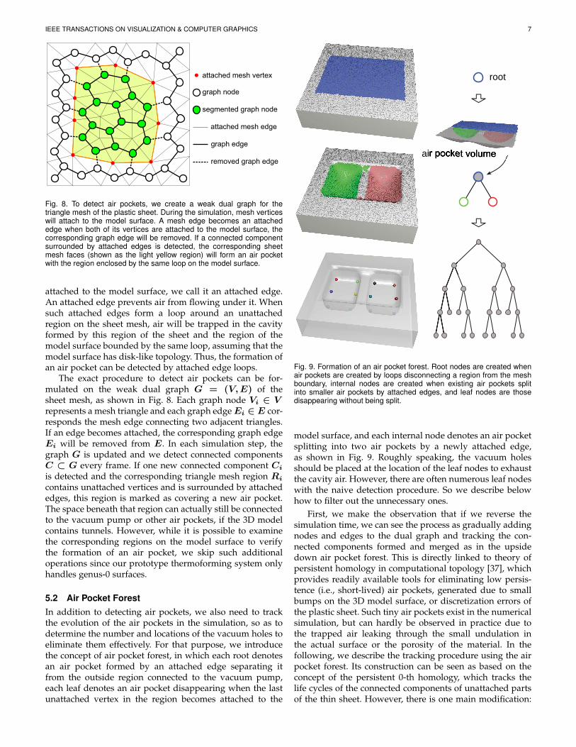
During the vacuum forming process of our virtual simu-lation, we assume that for all points on the plastic sheetthat have not yet reached the model surface, the pressuredifferences between the two sides of the sheet are the same.However, this assumption is only approximately true whenall spaces between the plastic sheet and the model areconnected to the vacuum pump. In practice, if the 3D modelsurface contains concave regions, for example, a large dent,it is highly likely that the rim of the dent will be covered bythe plastic sheet during the process, leaving the air trappedinside the dent, as shown in Fig. 7. To prevent this fromhappening, we need to detect potential air pockets duringthe virtual simulation and compute a layout of vacuumholes (also called vent holes) at the bottom of these regions.Air can then be sucked out through these channels, allowingthe plastic sheet to adhere to the model surface tightly.

5.1 Air Pocket DetectionAir pockets are formed between the triangle mesh of thesheet and the target surface, but we can actually detect theirformation directly on the sheet mesh during the simulation.In any simulation step in the vacuum forming stage, if avertex of the sheet touches the model surface, it will be at-tached there permanently. When both vertices of an edge are

(a) (b) (c)

Fig. 7. We compare the forming results of a concave model with andwithout vacuum holes: (a) the mold used for thermoforming, (b) if novacuum holes are set on the mold, air will be trapped in concave regions,and (c) after vacuum holes are drilled or preset before printing the mold,air will be exhausted through these holes and the plastic sheet willadhere tightly to the mold surface.


attached mesh vertex

graph node

segmented graph node

attached mesh edge

graph edge

removed graph edge

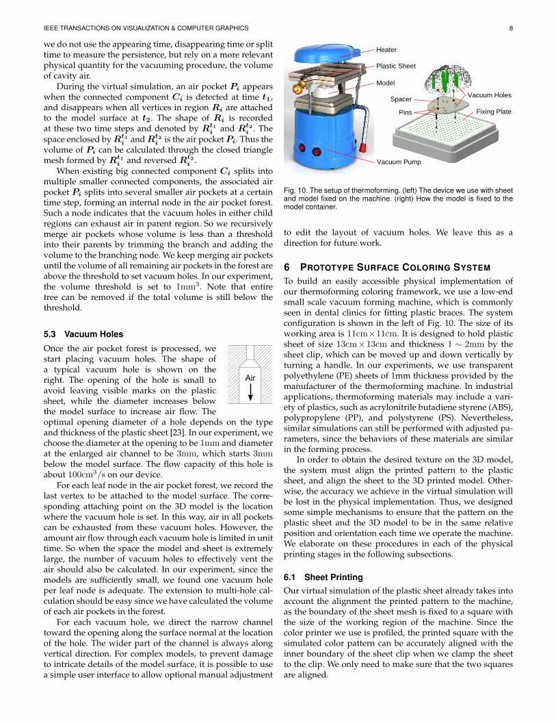
Fig. 8. To detect air pockets, we create a weak dual graph for thetriangle mesh of the plastic sheet. During the simulation, mesh verticeswill attach to the model surface. A mesh edge becomes an attachededge when both of its vertices are attached to the model surface, thecorresponding graph edge will be removed. If a connected componentsurrounded by attached edges is detected, the corresponding sheetmesh faces (shown as the light yellow region) will form an air pocketwith the region enclosed by the same loop on the model surface.

attached to the model surface, we call it an attached edge.An attached edge prevents air from flowing under it. Whensuch attached edges form a loop around an unattachedregion on the sheet mesh, air will be trapped in the cavityformed by this region of the sheet and the region of themodel surface bounded by the same loop, assuming that themodel surface has disk-like topology. Thus, the formation ofan air pocket can be detected by attached edge loops.

The exact procedure to detect air pockets can be for-mulated on the weak dual graph G = (V,E) of thesheet mesh, as shown in Fig. 8. Each graph node Vi ∈ Vrepresents a mesh triangle and each graph edgeEi ∈ E cor-responds the mesh edge connecting two adjacent triangles.If an edge becomes attached, the corresponding graph edgeEi will be removed from E. In each simulation step, thegraph G is updated and we detect connected componentsC ⊂ G every frame. If one new connected component Ci

is detected and the corresponding triangle mesh region Ri

contains unattached vertices and is surrounded by attachededges, this region is marked as covering a new air pocket.The space beneath that region can actually still be connectedto the vacuum pump or other air pockets, if the 3D modelcontains tunnels. However, while it is possible to examinethe corresponding regions on the model surface to verifythe formation of an air pocket, we skip such additionaloperations since our prototype thermoforming system onlyhandles genus-0 surfaces.

5.2 Air Pocket ForestIn addition to detecting air pockets, we also need to trackthe evolution of the air pockets in the simulation, so as todetermine the number and locations of the vacuum holes toeliminate them effectively. For that purpose, we introducethe concept of air pocket forest, in which each root denotesan air pocket formed by an attached edge separating itfrom the outside region connected to the vacuum pump,each leaf denotes an air pocket disappearing when the lastunattached vertex in the region becomes attached to the

air pocket volume

root

Fig. 9. Formation of an air pocket forest. Root nodes are created whenair pockets are created by loops disconnecting a region from the meshboundary, internal nodes are created when existing air pockets splitinto smaller air pockets by attached edges, and leaf nodes are thosedisappearing without being split.

model surface, and each internal node denotes an air pocketsplitting into two air pockets by a newly attached edge,as shown in Fig. 9. Roughly speaking, the vacuum holesshould be placed at the location of the leaf nodes to exhaustthe cavity air. However, there are often numerous leaf nodeswith the naive detection procedure. So we describe belowhow to filter out the unnecessary ones.

First, we make the observation that if we reverse thesimulation time, we can see the process as gradually addingnodes and edges to the dual graph and tracking the con-nected components formed and merged as in the upsidedown air pocket forest. This is directly linked to theory ofpersistent homology in computational topology [37], whichprovides readily available tools for eliminating low persis-tence (i.e., short-lived) air pockets, generated due to smallbumps on the 3D model surface, or discretization errors ofthe plastic sheet. Such tiny air pockets exist in the numericalsimulation, but can hardly be observed in practice due tothe trapped air leaking through the small undulation inthe actual surface or the porosity of the material. In thefollowing, we describe the tracking procedure using the airpocket forest. Its construction can be seen as based on theconcept of the persistent 0-th homology, which tracks thelife cycles of the connected components of unattached partsof the thin sheet. However, there is one main modification:


we do not use the appearing time, disappearing time or splittime to measure the persistence, but rely on a more relevantphysical quantity for the vacuuming procedure, the volumeof cavity air.

During the virtual simulation, an air pocket Pi appearswhen the connected component Ci is detected at time t1,and disappears when all vertices in region Ri are attachedto the model surface at t2. The shape of Ri is recordedat these two time steps and denoted by Rt1

i and Rt2i . The

space enclosed byRt1i andRt2

i is the air pocketPi. Thus thevolume of Pi can be calculated through the closed trianglemesh formed by Rt1

i and reversed Rt2i .

When existing big connected component Ci splits intomultiple smaller connected components, the associated airpocket Pi splits into several smaller air pockets at a certaintime step, forming an internal node in the air pocket forest.Such a node indicates that the vacuum holes in either childregions can exhaust air in parent region. So we recursivelymerge air pockets whose volume is less than a thresholdinto their parents by trimming the branch and adding thevolume to the branching node. We keep merging air pocketsuntil the volume of all remaining air pockets in the forest areabove the threshold to set vacuum holes. In our experiment,the volume threshold is set to 1mm3. Note that entiretree can be removed if the total volume is still below thethreshold.

5.3 Vacuum Holes

Air

Once the air pocket forest is processed, westart placing vacuum holes. The shape ofa typical vacuum hole is shown on theright. The opening of the hole is small toavoid leaving visible marks on the plasticsheet, while the diameter increases belowthe model surface to increase air flow. Theoptimal opening diameter of a hole depends on the typeand thickness of the plastic sheet [23]. In our experiment, wechoose the diameter at the opening to be 1mm and diameterat the enlarged air channel to be 3mm, which starts 3mmbelow the model surface. The flow capacity of this hole isabout 100cm3/s on our device.

For each leaf node in the air pocket forest, we record thelast vertex to be attached to the model surface. The corre-sponding attaching point on the 3D model is the locationwhere the vacuum hole is set. In this way, air in all pocketscan be exhausted from these vacuum holes. However, theamount air flow through each vacuum hole is limited in unittime. So when the space the model and sheet is extremelylarge, the number of vacuum holes to effectively vent theair should also be calculated. In our experiment, since themodels are sufficiently small, we found one vacuum holeper leaf node is adequate. The extension to multi-hole cal-culation should be easy since we have calculated the volumeof each air pockets in the forest.

For each vacuum hole, we direct the narrow channeltoward the opening along the surface normal at the locationof the hole. The wider part of the channel is always alongvertical direction. For complex models, to prevent damageto intricate details of the model surface, it is possible to usea simple user interface to allow optional manual adjustment

Heater

Plastic Sheet

Model

Vacuum Pump

Spacer

Pins

Vacuum Holes

Fixing Plate

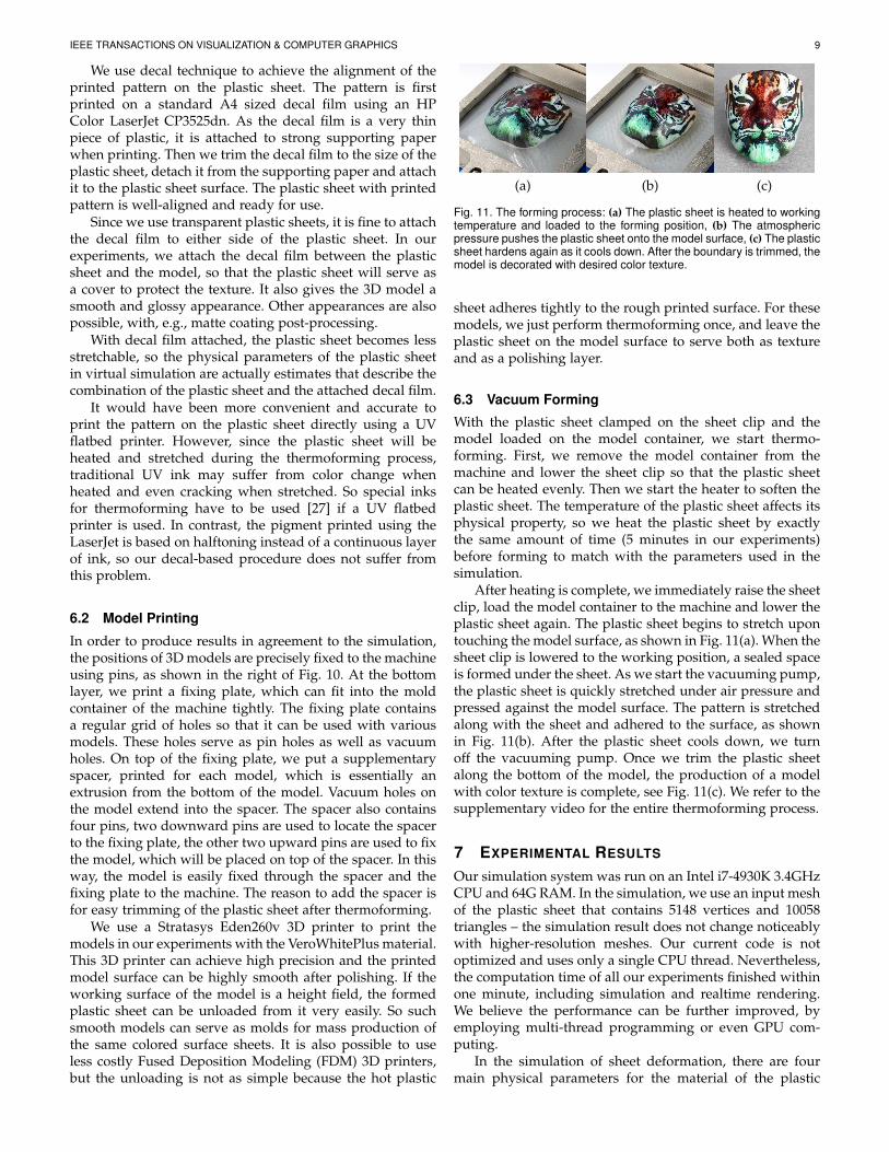
Fig. 10. The setup of thermoforming. (left) The device we use with sheetand model fixed on the machine. (right) How the model is fixed to themodel container.

to edit the layout of vacuum holes. We leave this as adirection for future work.

6 PROTOTYPE SURFACE COLORING SYSTEM

To build an easily accessible physical implementation ofour thermoforming coloring framework, we use a low-endsmall scale vacuum forming machine, which is commonlyseen in dental clinics for fitting plastic braces. The systemconfiguration is shown in the left of Fig. 10. The size of itsworking area is 11cm×11cm. It is designed to hold plasticsheet of size 13cm×13cm and thickness 1 ∼ 2mm by thesheet clip, which can be moved up and down vertically byturning a handle. In our experiments, we use transparentpolyethylene (PE) sheets of 1mm thickness provided by themanufacturer of the thermoforming machine. In industrialapplications, thermoforming materials may include a vari-ety of plastics, such as acrylonitrile butadiene styrene (ABS),polypropylene (PP), and polystyrene (PS). Nevertheless,similar simulations can still be performed with adjusted pa-rameters, since the behaviors of these materials are similarin the forming process.

In order to obtain the desired texture on the 3D model,the system must align the printed pattern to the plasticsheet, and align the sheet to the 3D printed model. Other-wise, the accuracy we achieve in the virtual simulation willbe lost in the physical implementation. Thus, we designedsome simple mechanisms to ensure that the pattern on theplastic sheet and the 3D model to be in the same relativeposition and orientation each time we operate the machine.We elaborate on these procedures in each of the physicalprinting stages in the following subsections.

6.1 Sheet PrintingOur virtual simulation of the plastic sheet already takes intoaccount the alignment the printed pattern to the machine,as the boundary of the sheet mesh is fixed to a square withthe size of the working region of the machine. Since thecolor printer we use is profiled, the printed square with thesimulated color pattern can be accurately aligned with theinner boundary of the sheet clip when we clamp the sheetto the clip. We only need to make sure that the two squaresare aligned.


We use decal technique to achieve the alignment of theprinted pattern on the plastic sheet. The pattern is firstprinted on a standard A4 sized decal film using an HPColor LaserJet CP3525dn. As the decal film is a very thinpiece of plastic, it is attached to strong supporting paperwhen printing. Then we trim the decal film to the size of theplastic sheet, detach it from the supporting paper and attachit to the plastic sheet surface. The plastic sheet with printedpattern is well-aligned and ready for use.

Since we use transparent plastic sheets, it is fine to attachthe decal film to either side of the plastic sheet. In ourexperiments, we attach the decal film between the plasticsheet and the model, so that the plastic sheet will serve asa cover to protect the texture. It also gives the 3D model asmooth and glossy appearance. Other appearances are alsopossible, with, e.g., matte coating post-processing.

With decal film attached, the plastic sheet becomes lessstretchable, so the physical parameters of the plastic sheetin virtual simulation are actually estimates that describe thecombination of the plastic sheet and the attached decal film.

It would have been more convenient and accurate toprint the pattern on the plastic sheet directly using a UVflatbed printer. However, since the plastic sheet will beheated and stretched during the thermoforming process,traditional UV ink may suffer from color change whenheated and even cracking when stretched. So special inksfor thermoforming have to be used [27] if a UV flatbedprinter is used. In contrast, the pigment printed using theLaserJet is based on halftoning instead of a continuous layerof ink, so our decal-based procedure does not suffer fromthis problem.

6.2 Model Printing

In order to produce results in agreement to the simulation,the positions of 3D models are precisely fixed to the machineusing pins, as shown in the right of Fig. 10. At the bottomlayer, we print a fixing plate, which can fit into the moldcontainer of the machine tightly. The fixing plate containsa regular grid of holes so that it can be used with variousmodels. These holes serve as pin holes as well as vacuumholes. On top of the fixing plate, we put a supplementaryspacer, printed for each model, which is essentially anextrusion from the bottom of the model. Vacuum holes onthe model extend into the spacer. The spacer also containsfour pins, two downward pins are used to locate the spacerto the fixing plate, the other two upward pins are used to fixthe model, which will be placed on top of the spacer. In thisway, the model is easily fixed through the spacer and thefixing plate to the machine. The reason to add the spacer isfor easy trimming of the plastic sheet after thermoforming.

We use a Stratasys Eden260v 3D printer to print themodels in our experiments with the VeroWhitePlus material.This 3D printer can achieve high precision and the printedmodel surface can be highly smooth after polishing. If theworking surface of the model is a height field, the formedplastic sheet can be unloaded from it very easily. So suchsmooth models can serve as molds for mass production ofthe same colored surface sheets. It is also possible to useless costly Fused Deposition Modeling (FDM) 3D printers,but the unloading is not as simple because the hot plastic

(a) (b) (c)

Fig. 11. The forming process: (a) The plastic sheet is heated to workingtemperature and loaded to the forming position, (b) The atmosphericpressure pushes the plastic sheet onto the model surface, (c) The plasticsheet hardens again as it cools down. After the boundary is trimmed, themodel is decorated with desired color texture.

sheet adheres tightly to the rough printed surface. For thesemodels, we just perform thermoforming once, and leave theplastic sheet on the model surface to serve both as textureand as a polishing layer.

6.3 Vacuum Forming

With the plastic sheet clamped on the sheet clip and themodel loaded on the model container, we start thermo-forming. First, we remove the model container from themachine and lower the sheet clip so that the plastic sheetcan be heated evenly. Then we start the heater to soften theplastic sheet. The temperature of the plastic sheet affects itsphysical property, so we heat the plastic sheet by exactlythe same amount of time (5 minutes in our experiments)before forming to match with the parameters used in thesimulation.

After heating is complete, we immediately raise the sheetclip, load the model container to the machine and lower theplastic sheet again. The plastic sheet begins to stretch upontouching the model surface, as shown in Fig. 11(a). When thesheet clip is lowered to the working position, a sealed spaceis formed under the sheet. As we start the vacuuming pump,the plastic sheet is quickly stretched under air pressure andpressed against the model surface. The pattern is stretchedalong with the sheet and adhered to the surface, as shownin Fig. 11(b). After the plastic sheet cools down, we turnoff the vacuuming pump. Once we trim the plastic sheetalong the bottom of the model, the production of a modelwith color texture is complete, see Fig. 11(c). We refer to thesupplementary video for the entire thermoforming process.

7 EXPERIMENTAL RESULTS

Our simulation system was run on an Intel i7-4930K 3.4GHzCPU and 64G RAM. In the simulation, we use an input meshof the plastic sheet that contains 5148 vertices and 10058triangles – the simulation result does not change noticeablywith higher-resolution meshes. Our current code is notoptimized and uses only a single CPU thread. Nevertheless,the computation time of all our experiments finished withinone minute, including simulation and realtime rendering.We believe the performance can be further improved, byemploying multi-thread programming or even GPU com-puting.

In the simulation of sheet deformation, there are fourmain physical parameters for the material of the plastic


sheet (attached with decal film): Young’s modulus, Pois-son’s ratio, initial yield stress and hardening coefficient.The value of the Young’s modulus (Y = 1MPa) at formingtemperature is provided by the plastic sheet manufacture.The Poisson’s ratio of polymers when passed yield pointis about 0.5 as mentioned in [39], which means that thematerial becomes incompressible when undergoing plasticdeformation. Since we have a relatively low yield stress andplastic deformation starts at a very early stage, we simplytreat the Poisson’s ratio (ν = 0.5) to be constant throughthe simulation. The value of initial yield stress (σ0 = 220Pa)and hardening coefficient (K = 1000Pa) are determined byexperiment. We use a plastic sheet printed with grid patternto perform a standard thermoforming procedure with atruncated cone (Sec. 7.1) as mold. Then, we perform a seriesof virtual simulations with different σ0 and K values andchoose the values that yield the best matching results to thereal experiment. We perform a single physical experiment,and multiple simulations with σ0 and K chosen from a20×20 combination of values. With the total running timeof about one hour, we can easily refine the parameters withanother round of 400 simulations based on the first roundestimates if necessary. It is also possible to scan the result ofreal experiment and select the best matching automatically,as described in [28].

The stiffness constant kr to control repulsive force incollision (Sec. 4.1.3) was manually set at kr = 5× 108N/m3.This coefficient needs to be sufficiently large to prevent anyvisible penetration in our experiments. The coefficient offriction µ depends both on the plastic sheet and the materialfor 3D printing. For the VeroWhitePlus material used bythe Stratasys Eden260v 3D printer, µ = 0.8 provides areasonable approximation in simulation. For models withvery rough surfaces, such as the ones printed using FDM3D printer, there is almost no visible slipping. In this case,we can further simplify the simulation by fixing the verticesas soon as they touch the surface of the 3D model.

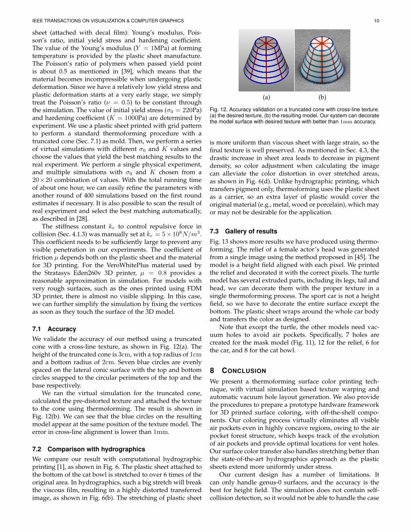
7.1 AccuracyWe validate the accuracy of our method using a truncatedcone with a cross-line texture, as shown in Fig. 12(a). Theheight of the truncated cone is 3cm, with a top radius of 1cmand a bottom radius of 2cm. Seven blue circles are evenlyspaced on the lateral conic surface with the top and bottomcircles snapped to the circular perimeters of the top and thebase respectively.

We ran the virtual simulation for the truncated cone,calculated the pre-distorted texture and attached the textureto the cone using thermoforming. The result is shown inFig. 12(b). We can see that the blue circles on the resultingmodel appear at the same position of the texture model. Theerror in cross-line alignment is lower than 1mm.

7.2 Comparison with hydrographicsWe compare our result with computational hydrographicprinting [1], as shown in Fig. 6. The plastic sheet attached tothe bottom of the cat bowl is stretched to over 6 times of theoriginal area. In hydrographics, such a big stretch will breakthe viscous film, resulting in a highly distorted transferredimage, as shown in Fig. 6(b). The stretching of plastic sheet

(a) (b)

Fig. 12. Accuracy validation on a truncated cone with cross-line texture.(a) the desired texture, (b) the resulting model. Our system can decoratethe model surface with desired texture with better than 1mm accuracy.

is more uniform than viscous sheet with large strain, so thefinal texture is well preserved. As mentioned in Sec. 4.3, thedrastic increase in sheet area leads to decrease in pigmentdensity, so color adjustment when calculating the imagecan alleviate the color distortion in over stretched areas,as shown in Fig. 6(d). Unlike hydrographic printing, whichtransfers pigment only, thermoforming uses the plastic sheetas a carrier, so an extra layer of plastic would cover theoriginal material (e.g., metal, wood or porcelain), which mayor may not be desirable for the application.

7.3 Gallery of results

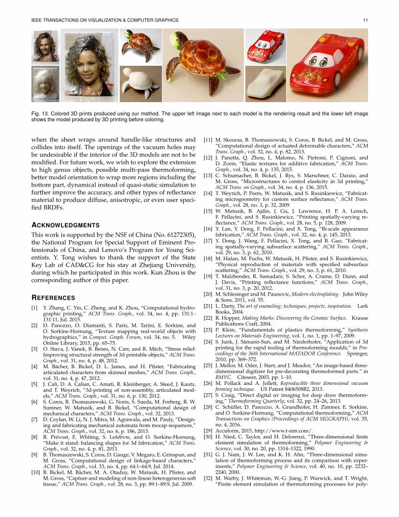
Fig. 13 shows more results we have produced using thermo-forming. The relief of a female actor’s head was generatedfrom a single image using the method proposed in [45]. Themodel is a height field aligned with each pixel. We printedthe relief and decorated it with the correct pixels. The turtlemodel has several extruded parts, including its legs, tail andhead, we can decorate them with the proper texture in asingle thermoforming process. The sport car is not a heightfield, so we have to decorate the entire surface except thebottom. The plastic sheet wraps around the whole car bodyand transfers the color as designed.

Note that except the turtle, the other models need vac-uum holes to avoid air pockets. Specifically, 7 holes arecreated for the mask model (Fig. 11), 12 for the relief, 6 forthe car, and 8 for the cat bowl.

8 CONCLUSION

We present a thermoforming surface color printing tech-nique, with virtual simulation based texture warping andautomatic vacuum hole layout generation. We also providethe procedures to prepare a prototype hardware frameworkfor 3D printed surface coloring, with off-the-shelf compo-nents. Our coloring process virtually eliminates all visibleair pockets even in highly concave regions, owing to the airpocket forest structure, which keeps track of the evolutionof air pockets and provide optimal locations for vent holes.Our surface color transfer also handles stretching better thanthe state-of-the-art hydrographics approach as the plasticsheets extend more uniformly under stress.

Our current design has a number of limitations. Itcan only handle genus-0 surfaces, and the accuracy is thebest for height field. The simulation does not contain self-collision detection, so it would not be able to handle the case


Fig. 13. Colored 3D prints produced using our method. The upper left image next to each model is the rendering result and the lower left imageshows the model produced by 3D printing before coloring.

when the sheet wraps around handle-like structures andcollides into itself. The openings of the vacuum holes maybe undesirable if the interior of the 3D models are not to bemodified. For future work, we wish to explore the extensionto high genus objects, possible multi-pass thermoforming,better model orientation to wrap more regions including thebottom part, dynamical instead of quasi-static simulation tofurther improve the accuracy, and other types of reflectancematerial to produce diffuse, anisotropic, or even user speci-fied BRDFs.

ACKNOWLEDGMENTS

This work is supported by the NSF of China (No. 61272305),the National Program for Special Support of Eminent Pro-fessionals of China, and Lenovo’s Program for Young Sci-entists. Y. Tong wishes to thank the support of the StateKey Lab of CAD&CG for his stay at Zhejiang University,during which he participated in this work. Kun Zhou is thecorresponding author of this paper.

REFERENCES

[1] Y. Zhang, C. Yin, C. Zheng, and K. Zhou, “Computational hydro-graphic printing,” ACM Trans. Graph., vol. 34, no. 4, pp. 131:1–131:11, Jul. 2015.

[2] D. Panozzo, O. Diamanti, S. Paris, M. Tarini, E. Sorkine, andO. Sorkine-Hornung, “Texture mapping real-world objects withhydrographics,” in Comput. Graph. Forum, vol. 34, no. 5. WileyOnline Library, 2015, pp. 65–75.

[3] O. Stava, J. Vanek, B. Benes, N. Carr, and R. Mech, “Stress relief:Improving structural strength of 3d printable objects,” ACM Trans.Graph., vol. 31, no. 4, p. 48, 2012.

[4] M. Bacher, B. Bickel, D. L. James, and H. Pfister, “Fabricatingarticulated characters from skinned meshes,” ACM Trans. Graph.,vol. 31, no. 4, p. 47, 2012.

[5] J. Calı, D. A. Calian, C. Amati, R. Kleinberger, A. Steed, J. Kautz,and T. Weyrich, “3d-printing of non-assembly, articulated mod-els,” ACM Trans. Graph., vol. 31, no. 6, p. 130, 2012.

[6] S. Coros, B. Thomaszewski, G. Noris, S. Sueda, M. Forberg, R. W.Sumner, W. Matusik, and B. Bickel, “Computational design ofmechanical characters,” ACM Trans. Graph., vol. 32, 2013.

[7] D. Ceylan, W. Li, N. J. Mitra, M. Agrawala, and M. Pauly, “Design-ing and fabricating mechanical automata from mocap sequences,”ACM Trans. Graph., vol. 32, no. 6, p. 186, 2013.

[8] R. Prevost, E. Whiting, S. Lefebvre, and O. Sorkine-Hornung,“Make it stand: balancing shapes for 3d fabrication,” ACM Trans.Graph., vol. 32, no. 4, p. 81, 2013.

[9] B. Thomaszewski, S. Coros, D. Gauge, V. Megaro, E. Grinspun, andM. Gross, “Computational design of linkage-based characters,”ACM Trans. Graph., vol. 33, no. 4, pp. 64:1–64:9, Jul. 2014.

[10] B. Bickel, M. Bacher, M. A. Otaduy, W. Matusik, H. Pfister, andM. Gross, “Capture and modeling of non-linear heterogeneous softtissue,” ACM Trans. Graph., vol. 28, no. 3, pp. 89:1–89:9, Jul. 2009.

[11] M. Skouras, B. Thomaszewski, S. Coros, B. Bickel, and M. Gross,“Computational design of actuated deformable characters,” ACMTrans. Graph., vol. 32, no. 4, p. 82, 2013.

[12] J. Panetta, Q. Zhou, L. Malomo, N. Pietroni, P. Cignoni, andD. Zorin, “Elastic textures for additive fabrication,” ACM Trans.Graph., vol. 34, no. 4, p. 135, 2015.

[13] C. Schumacher, B. Bickel, J. Rys, S. Marschner, C. Daraio, andM. Gross, “Microstructures to control elasticity in 3d printing,”ACM Trans. on Graph., vol. 34, no. 4, p. 136, 2015.

[14] T. Weyrich, P. Peers, W. Matusik, and S. Rusinkiewicz, “Fabricat-ing microgeometry for custom surface reflectance,” ACM Trans.Graph., vol. 28, no. 3, p. 32, 2009.

[15] W. Matusik, B. Ajdin, J. Gu, J. Lawrence, H. P. A. Lensch,F. Pellacini, and S. Rusinkiewicz, “Printing spatially-varying re-flectance,” ACM Trans. Graph., vol. 28, no. 5, p. 128, 2009.

[16] Y. Lan, Y. Dong, F. Pellacini, and X. Tong, “Bi-scale appearancefabrication,” ACM Trans. Graph., vol. 32, no. 4, p. 145, 2013.

[17] Y. Dong, J. Wang, F. Pellacini, X. Tong, and B. Guo, “Fabricat-ing spatially-varying subsurface scattering,” ACM Trans. Graph.,vol. 29, no. 3, p. 62, 2010.

[18] M. Hasan, M. Fuchs, W. Matusik, H. Pfister, and S. Rusinkiewicz,“Physical reproduction of materials with specified subsurfacescattering,” ACM Trans. Graph., vol. 29, no. 3, p. 61, 2010.

[19] T. Malzbender, R. Samadani, S. Scher, A. Crume, D. Dunn, andJ. Davis, “Printing reflectance functions,” ACM Trans. Graph.,vol. 31, no. 3, p. 20, 2012.

[20] M. Schlesinger and M. Paunovic, Modern electroplating. John Wiley& Sons, 2011, vol. 55.

[21] L. Darty, The art of enameling: techniques, projects, inspiration. LarkBooks, 2004.

[22] R. Hopper, Making Marks: Discovering the Ceramic Surface. KrausePublications Craft, 2004.

[23] P. Klein, “Fundamentals of plastics thermoforming,” SynthesisLectures on Materials Engineering, vol. 1, no. 1, pp. 1–97, 2009.

[24] S. Junk, J. Samann-Sun, and M. Niederhofer, “Application of 3dprinting for the rapid tooling of thermoforming moulds,” in Pro-ceedings of the 36th International MATADOR Conference. Springer,2010, pp. 369–372.

[25] J. Mellor, M. Oder, J. Starr, and J. Meador, “An image-based three-dimensional digitizer for pre-decorating thermoformed parts.” inBMVC. Citeseer, 2003, pp. 1–10.

[26] M. Pollack and A. Jollett, Reproducible three dimensional vacuumforming technique. US Patent 8406508B2, 2013.

[27] S. Craig, “Direct digital uv imaging for deep draw thermoform-ing,” Thermoforming Quarterly, vol. 32, pp. 24–26, 2013.

[28] C. Schuller, D. Panozzo, A. Grundhofer, H. Zimmer, E. Sorkine,and O. Sorkine-Hornung, “Computational thermoforming,” ACMTransactions on Graphics (Proceedings of ACM SIGGRAPH), vol. 35,no. 4, 2016.

[29] Accuform, 2015, http://www.t-sim.com/.[30] H. Nied, C. Taylor, and H. Delorenzi, “Three-dimensional finite

element simulation of thermoforming,” Polymer Engineering &Science, vol. 30, no. 20, pp. 1314–1322, 1990.

[31] G. J. Nam, J. W. Lee, and K. H. Ahn, “Three-dimensional simu-lation of thermoforming process and its comparison with exper-iments,” Polymer Engineering & Science, vol. 40, no. 10, pp. 2232–2240, 2000.

[32] M. Warby, J. Whiteman, W.-G. Jiang, P. Warwick, and T. Wright,“Finite element simulation of thermoforming processes for poly-


mer sheets,” Mathematics and computers in simulation, vol. 61, no. 3,pp. 209–218, 2003.

[33] J. Dees, FEA Simulations of Thermoforming–Using Hyperelastic Ma-terial Properties. Engineering simulations LLC, scientific article,2009.

[34] A. W. Bargteil, C. Wojtan, J. K. Hodgins, and G. Turk, “A finiteelement method for animating large viscoplastic flow,” ACMTrans. Graph., vol. 26, no. 3, Jul. 2007.

[35] C. Wojtan and G. Turk, “Fast viscoelastic behavior with thinfeatures,” ACM Trans. Graph., vol. 27, no. 3, pp. 47:1–47:8, Aug.2008.

[36] T. Pfaff, R. Narain, J. M. de Joya, and J. F. O’Brien, “Adaptivetearing and cracking of thin sheets,” ACM Trans. Graph., vol. 33,no. 4, pp. 110:1–110:9, Jul. 2014.

[37] H. Edelsbrunner and J. Harer, Computational topology: an introduc-tion. American Mathematical Soc., 2010.

[38] C. Park, H. Huh, J. Kim, and C. Ahn, “Determination of truestress–true strain curves of polymers at various strain rates usingforce equilibrium grid method,” Journal of Composite Materials,vol. 46, no. 17, pp. 2065–2077, 2012.

[39] R. Park, M. Priestley, and W. Walpole, “The seismic performanceof steel encased reinforced concrete bridge piles,” 1982.

[40] M. A. Meyers and K. K. Chawla, Mechanical behavior of materials.Cambridge university press Cambridge, 2009, vol. 2.

[41] Y. Yue, B. Smith, C. Batty, C. Zheng, and E. Grinspun, “Continuumfoam: A material point method for shear-dependent flows,” ACMTrans. Graph., vol. 34, no. 5, pp. 160:1–160:20, Nov. 2015.

[42] A. Fuhrmann, G. Sobotka, and C. Groß, “Distance fields for rapidcollision detection in physically based modeling,” in Proceedings ofGraphiCon 2003, 2003, pp. 58–65.

[43] R. Bridson, R. Fedkiw, and J. Anderson, “Robust treatment ofcollisions, contact and friction for cloth animation,” in ACM Trans.Graph., vol. 21, no. 3. ACM, 2002, pp. 594–603.

[44] J. R. Shewchuk, “Triangle: Engineering a 2d quality mesh gener-ator and delaunay triangulator,” in Applied computational geometrytowards geometric engineering. Springer, 1996, pp. 203–222.

[45] M. Chai, L. Luo, K. Sunkavalli, N. Carr, S. Hadap, and K. Zhou,“High-quality hair modeling from a single portrait photo,” ACMTrans. Graph., vol. 34, no. 6, pp. 204:1–204:10, Oct. 2015.

Yizhong Zhang is a Ph.D. student in the statekey laboratory of CAD&CG, Zhejiang University,Hangzhou, China. He received his B.S. degreein Mechatronics Engineering from Zhejiang Uni-versity in 2010. His research interests includephysically based simulation, computer graphics,computational fabrication and robotics.

Yiying Tong is an associate professor at Michi-gan State University. He received his Ph.D. de-gree from University of Southern California in2004. His research interests include discretegeometric modeling, physically-based simula-tion/animation, and discrete differential geome-try. He received the U.S. National Science Foun-dation (NSF) Career Award in 2010.

Kun Zhou is a Cheung Kong Professor in theComputer Science Department of Zhejiang Uni-versity, and the Director of the State Key Labof CAD&CG. Prior to joining Zhejiang Universityin 2008, Dr. Zhou was a Leader Researcher ofthe Internet Graphics Group at Microsoft Re-search Asia. He received his B.S. degree andPh.D. degree in computer science from ZhejiangUniversity in 1997 and 2002, respectively. Hisresearch interests are in visual computing, paral-lel computing, human computer interaction, and

virtual reality. He currently serves on the editorial/advisory boards ofACM Transactions on Graphics and IEEE Spectrum. He is a Fellow ofIEEE.

ieee transactions on visualization & computer graphics...

Documents