ieor 269, spring 2010 integer programming and combinatorial...
TRANSCRIPT

IEOR 269, Spring 2010
Integer Programming and Combinatorial Optimization
Professor Dorit S. Hochbaum
Contents
1 Introduction 1
2 Formulation of some ILP 22.1 0-1 knapsack problem . . . . . . . . . . . . . . . . . . . . . . . . . . . . . . . . . . . 22.2 Assignment problem . . . . . . . . . . . . . . . . . . . . . . . . . . . . . . . . . . . . 2
3 Non-linear Objective functions 43.1 Production problem with set-up costs . . . . . . . . . . . . . . . . . . . . . . . . . . 43.2 Piecewise linear cost function . . . . . . . . . . . . . . . . . . . . . . . . . . . . . . . 53.3 Piecewise linear convex cost function . . . . . . . . . . . . . . . . . . . . . . . . . . . 63.4 Disjunctive constraints . . . . . . . . . . . . . . . . . . . . . . . . . . . . . . . . . . . 7
4 Some famous combinatorial problems 74.1 Max clique problem . . . . . . . . . . . . . . . . . . . . . . . . . . . . . . . . . . . . 74.2 SAT (satisfiability) . . . . . . . . . . . . . . . . . . . . . . . . . . . . . . . . . . . . . 74.3 Vertex cover problem . . . . . . . . . . . . . . . . . . . . . . . . . . . . . . . . . . . . 7
5 General optimization 8
6 Neighborhood 86.1 Exact neighborhood . . . . . . . . . . . . . . . . . . . . . . . . . . . . . . . . . . . . 8
7 Complexity of algorithms 97.1 Finding the maximum element . . . . . . . . . . . . . . . . . . . . . . . . . . . . . . 97.2 0-1 knapsack . . . . . . . . . . . . . . . . . . . . . . . . . . . . . . . . . . . . . . . . 97.3 Linear systems . . . . . . . . . . . . . . . . . . . . . . . . . . . . . . . . . . . . . . . 107.4 Linear Programming . . . . . . . . . . . . . . . . . . . . . . . . . . . . . . . . . . . . 11
8 Some interesting IP formulations 128.1 The fixed cost plant location problem . . . . . . . . . . . . . . . . . . . . . . . . . . 128.2 Minimum/maximum spanning tree (MST) . . . . . . . . . . . . . . . . . . . . . . . . 12
9 The Minimum Spanning Tree (MST) Problem 13
i

IEOR269 notes, Prof. Hochbaum, 2010 ii
10 General Matching Problem 1410.1 Maximum Matching Problem in Bipartite Graphs . . . . . . . . . . . . . . . . . . . . 1410.2 Maximum Matching Problem in Non-Bipartite Graphs . . . . . . . . . . . . . . . . . 1510.3 Constraint Matrix Analysis for Matching Problems . . . . . . . . . . . . . . . . . . . 16
11 Traveling Salesperson Problem (TSP) 1711.1 IP Formulation for TSP . . . . . . . . . . . . . . . . . . . . . . . . . . . . . . . . . . 17
12 Discussion of LP-Formulation for MST 18
13 Branch-and-Bound 2013.1 The Branch-and-Bound technique . . . . . . . . . . . . . . . . . . . . . . . . . . . . 2013.2 Other Branch-and-Bound techniques . . . . . . . . . . . . . . . . . . . . . . . . . . . 22
14 Basic graph definitions 23
15 Complexity analysis 2415.1 Measuring quality of an algorithm . . . . . . . . . . . . . . . . . . . . . . . . . . . . 24
15.1.1 Examples . . . . . . . . . . . . . . . . . . . . . . . . . . . . . . . . . . . . . . 2415.2 Growth of functions . . . . . . . . . . . . . . . . . . . . . . . . . . . . . . . . . . . . 2615.3 Definitions for asymptotic comparisons of functions . . . . . . . . . . . . . . . . . . . 2615.4 Properties of asymptotic notation . . . . . . . . . . . . . . . . . . . . . . . . . . . . . 2615.5 Caveats of complexity analysis . . . . . . . . . . . . . . . . . . . . . . . . . . . . . . 27
16 Complexity classes and NP-completeness 2816.1 Search vs. Decision . . . . . . . . . . . . . . . . . . . . . . . . . . . . . . . . . . . . . 2816.2 The class NP . . . . . . . . . . . . . . . . . . . . . . . . . . . . . . . . . . . . . . . . 29
17 Addendum on Branch and Bound 30
18 Complexity classes and NP-completeness 3118.1 Search vs. Decision . . . . . . . . . . . . . . . . . . . . . . . . . . . . . . . . . . . . . 3118.2 The class NP . . . . . . . . . . . . . . . . . . . . . . . . . . . . . . . . . . . . . . . . 32
18.2.1 Some Problems in NP . . . . . . . . . . . . . . . . . . . . . . . . . . . . . . . 3318.3 The class co-NP . . . . . . . . . . . . . . . . . . . . . . . . . . . . . . . . . . . . . . 34
18.3.1 Some Problems in co-NP . . . . . . . . . . . . . . . . . . . . . . . . . . . . . 3418.4 NPand co-NP . . . . . . . . . . . . . . . . . . . . . . . . . . . . . . . . . . . . . . . . 3418.5 NP-completeness and reductions . . . . . . . . . . . . . . . . . . . . . . . . . . . . . 35
18.5.1 Reducibility . . . . . . . . . . . . . . . . . . . . . . . . . . . . . . . . . . . . . 3518.5.2 NP-Completeness . . . . . . . . . . . . . . . . . . . . . . . . . . . . . . . . . . 36
19 The Chinese Checkerboard Problem and a First Look at Cutting Planes 4019.1 Problem Setup . . . . . . . . . . . . . . . . . . . . . . . . . . . . . . . . . . . . . . . 4019.2 The First Integer Programming Formulation . . . . . . . . . . . . . . . . . . . . . . . 4019.3 An Improved ILP Formulation . . . . . . . . . . . . . . . . . . . . . . . . . . . . . . 40
20 Cutting Planes 4320.1 Chinese checkers . . . . . . . . . . . . . . . . . . . . . . . . . . . . . . . . . . . . . . 4320.2 Branch and Cut . . . . . . . . . . . . . . . . . . . . . . . . . . . . . . . . . . . . . . . 44

IEOR269 notes, Prof. Hochbaum, 2010 iii
21 The geometry of Integer Programs and Linear Programs 4521.1 Cutting planes for the Knapsack problem . . . . . . . . . . . . . . . . . . . . . . . . 4521.2 Cutting plane approach for the TSP . . . . . . . . . . . . . . . . . . . . . . . . . . . 46
22 Gomory cuts 46
23 Generating a Feasible Solution for TSP 47
24 Diophantine Equations 4824.1 Hermite Normal Form . . . . . . . . . . . . . . . . . . . . . . . . . . . . . . . . . . . 49
25 Optimization with linear set of equality constraints 51
26 Balas’s additive algorithm 51
27 Held and Karp’s algorithm for TSP 54
28 Lagrangian Relaxation 55
29 Lagrangian Relaxation 59
30 Complexity of Nonlinear Optimization 6130.1 Input for a Polynomial Function . . . . . . . . . . . . . . . . . . . . . . . . . . . . . 6130.2 Table Look-Up . . . . . . . . . . . . . . . . . . . . . . . . . . . . . . . . . . . . . . . 6130.3 Examples of Non-linear Optimization Problems . . . . . . . . . . . . . . . . . . . . . 6230.4 Impossibility of strongly polynomial algorithms for nonlinear (non-quadratic) opti-
mization . . . . . . . . . . . . . . . . . . . . . . . . . . . . . . . . . . . . . . . . . . . 64
31 The General Network Flow Problem Setup 65
32 Shortest Path Problem 68
33 Maximum Flow Problem 6933.1 Setup . . . . . . . . . . . . . . . . . . . . . . . . . . . . . . . . . . . . . . . . . . . . 6933.2 Algorithms . . . . . . . . . . . . . . . . . . . . . . . . . . . . . . . . . . . . . . . . . 71
33.2.1 Ford-Fulkerson algorithm . . . . . . . . . . . . . . . . . . . . . . . . . . . . . 7233.2.2 Capacity scaling algorithm . . . . . . . . . . . . . . . . . . . . . . . . . . . . 74
33.3 Maximum-flow versus Minimum Cost Network Flow . . . . . . . . . . . . . . . . . . 7533.4 Formulation . . . . . . . . . . . . . . . . . . . . . . . . . . . . . . . . . . . . . . . . . 75
34 Minimum Cut Problem 7734.1 Minimum s-t Cut Problem . . . . . . . . . . . . . . . . . . . . . . . . . . . . . . . . . 7734.2 Formulation . . . . . . . . . . . . . . . . . . . . . . . . . . . . . . . . . . . . . . . . . 78
35 Selection Problem 79
36 A Production/Distribution Network: MCNF Formulation 8136.1 Problem Description . . . . . . . . . . . . . . . . . . . . . . . . . . . . . . . . . . . . 8136.2 Formulation as a Minimum Cost Network Flow Problem . . . . . . . . . . . . . . . . 8336.3 The Optimal Solution to the Chairs Problem . . . . . . . . . . . . . . . . . . . . . . 84

IEOR269 notes, Prof. Hochbaum, 2010 iv
37 Transhipment Problem 87
38 Transportation Problem 8738.1 Production/Inventory Problem as Transportation Problem . . . . . . . . . . . . . . . 88
39 Assignment Problem 90
40 Maximum Flow Problem 9040.1 A Package Delivery Problem . . . . . . . . . . . . . . . . . . . . . . . . . . . . . . . 90
41 Shortest Path Problem 9141.1 An Equipment Replacement Problem . . . . . . . . . . . . . . . . . . . . . . . . . . . 92
42 Maximum Weight Matching 9342.1 An Agent Scheduling Problem with Reassignment . . . . . . . . . . . . . . . . . . . 93
43 MCNF Hierarchy 96
44 The maximum/minimum closure problem 9644.1 A practical example: open-pit mining . . . . . . . . . . . . . . . . . . . . . . . . . . 9644.2 The maximum closure problem . . . . . . . . . . . . . . . . . . . . . . . . . . . . . . 98
45 Integer programs with two variables per inequality 10145.1 Monotone IP2 . . . . . . . . . . . . . . . . . . . . . . . . . . . . . . . . . . . . . . . . 10145.2 Non–monotone IP2 . . . . . . . . . . . . . . . . . . . . . . . . . . . . . . . . . . . . . 103
46 Vertex cover problem 10446.1 Vertex cover on bipartite graphs . . . . . . . . . . . . . . . . . . . . . . . . . . . . . 10546.2 Vertex cover on general graphs . . . . . . . . . . . . . . . . . . . . . . . . . . . . . . 105
47 The convex cost closure problem 10747.1 The threshold theorem . . . . . . . . . . . . . . . . . . . . . . . . . . . . . . . . . . . 10847.2 Naive algorithm for solving (ccc) . . . . . . . . . . . . . . . . . . . . . . . . . . . . . 11147.3 Solving (ccc) in polynomial time using binary search . . . . . . . . . . . . . . . . . . 11147.4 Solving (ccc) using parametric minimum cut . . . . . . . . . . . . . . . . . . . . . . . 111
48 The s-excess problem 11348.1 The convex s-excess problem . . . . . . . . . . . . . . . . . . . . . . . . . . . . . . . 11448.2 Threshold theorem for linear edge weights . . . . . . . . . . . . . . . . . . . . . . . . 11448.3 Variants / special cases . . . . . . . . . . . . . . . . . . . . . . . . . . . . . . . . . . 115
49 Forest Clearing 116
50 Producing memory chips (VLSI layout) 117
51 Independent set problem 11751.1 Independent Set v.s. Vertex Cover . . . . . . . . . . . . . . . . . . . . . . . . . . . . 11851.2 Independent set on bipartite graphs . . . . . . . . . . . . . . . . . . . . . . . . . . . 118

IEOR269 notes, Prof. Hochbaum, 2010 v
52 Maximum Density Subgraph 11952.1 Linearizing ratio problems . . . . . . . . . . . . . . . . . . . . . . . . . . . . . . . . . 11952.2 Solving the maximum density subgraph problem . . . . . . . . . . . . . . . . . . . . 119
53 Parametric cut/flow problem 12053.1 The parametric cut/flow problem with convex function (tentative title) . . . . . . . 121
54 Average k-cut problem 122
55 Image segmentation problem 12255.1 Solving the normalized cut variant problem . . . . . . . . . . . . . . . . . . . . . . . 12355.2 Solving the λ-question with a minimum cut procedure . . . . . . . . . . . . . . . . . 125
56 Duality of Max-Flow and MCNF Problems 12756.1 Duality of Max-Flow Problem: Minimum Cut . . . . . . . . . . . . . . . . . . . . . . 12756.2 Duality of MCNF problem . . . . . . . . . . . . . . . . . . . . . . . . . . . . . . . . . 127
57 Variant of Normalized Cut Problem 12857.1 Problem Setup . . . . . . . . . . . . . . . . . . . . . . . . . . . . . . . . . . . . . . . 12957.2 Review of Maximum Closure Problem . . . . . . . . . . . . . . . . . . . . . . . . . . 13057.3 Review of Maximum s-Excess Problem . . . . . . . . . . . . . . . . . . . . . . . . . . 13157.4 Relationship between s-excess and maximum closure problems . . . . . . . . . . . . 13257.5 Solution Approach for Variant of the Normalized Cut problem . . . . . . . . . . . . 132
58 Markov Random Fields 133
59 Examples of 2 vs. 3 in Combinatorial Optimization 13459.1 Edge Packing vs. Vertex Packing . . . . . . . . . . . . . . . . . . . . . . . . . . . . 13459.2 Chinese Postman Problem vs. Traveling Salesman Problem . . . . . . . . . . . . . . 13559.3 2SAT vs. 3SAT . . . . . . . . . . . . . . . . . . . . . . . . . . . . . . . . . . . . . . . 13659.4 Even Multivertex Cover vs. Vertex Cover . . . . . . . . . . . . . . . . . . . . . . . . 13659.5 Edge Cover vs. Vertex Cover . . . . . . . . . . . . . . . . . . . . . . . . . . . . . . . 13759.6 IP Feasibility: 2 vs. 3 Variables per Inequality . . . . . . . . . . . . . . . . . . . . . 138
These notes are based on “scribe” notes taken by students attending Professor Hochbaum’s courseIEOR 269 in the spring semester of 2010. The current version has been updated and edited byProfessor Hochbaum 2010
IEOR269 notes, Prof. Hochbaum, 2010 1
Lec1
1 Introduction
Consider the general form of a linear program:
max∑n
i=1 cixi
subject to Ax ≤ b
In an integer programming optimization problem, the additional restriction that the xi must beinteger-valued is also present.
While at first it may seem that the integrality condition limits the number of possible solutionsand could thereby make the integer problem easier than the continuous problem, the opposite isactually true. Linear programming optimization problems have the property that there exists anoptimal solution at a so-called extreme point (a basic solution); the optimal solution in an integerprogram, however, is not guaranteed to satisfy any such property and the number of possible integervalued solutions to consider becomes prohibitively large, in general.
While linear programming belongs to the class of problems P for which “good” algorithms exist(an algorithm is said to be good if its running time is bounded by a polynomial in the size of theinput), integer programming belongs to the class of NP-hard problems for which it is consideredhighly unlikely that a “good” algorithm exists. For some integer programming problems, such asthe Assignment Problem (which is described later in this lecture), efficient algorithms do exist.Unlike linear programming, however, for which effective general purpose solution techniques exist(ex. simplex method, ellipsoid method, Karmarkar’s algorithm), integer programming problemstend to be best handled in an ad hoc manner. While there are general techniques for dealing withinteger programs (ex. branch-and-bound, simulated annealing, cutting planes), it is usually betterto take advantage of the structure of the specific integer programming problems you are dealingwith and to develop special purposes approaches to take advantage of this particular structure.
Thus, it is important to become familiar with a wide variety of different classes of integerprogramming problems. Gaining such an understanding will be useful when you are later confrontedwith a new integer programming problem and have to determine how best to deal with it. Thiswill be a main focus of this course.
One natural idea for solving an integer program is to first solve the “LP-relaxation” of theproblem (ignore the integrality constraints), and then round the solution. As indicated in the classhandout, there are several fundamental problems to using this as a general approach:
1. The rounded solutions may not be feasible.
2. The rounded solutions, even if some are feasible, may not contain the optimal solution. Thesolutions of the ILP in general can be arbitrarily far from the solutions of the LP.
3. Even if one of the rounded solutions is optimal, checking all roundings is computationallyexpensive. There are 2n possible roundings to consider for an n variable problem, whichbecomes prohibitive for even moderate sized n.

IEOR269 notes, Prof. Hochbaum, 2010 2
2 Formulation of some ILP
2.1 0-1 knapsack problem
Given n items with utility ui and weight wi for i ∈ 1, . . . , n, find of subset of items with maximalutility under a weight constraint B. To formulate the problem as an ILP, the variable xi, i = 1, . . . , nis defined as follows:
xi =
1 if item i is selected0 otherwise
and the problem can be formulated as:
maxn∑i=1
uixi
subject ton∑i=1
wi xi ≤ B
xi ∈ 0, 1, i ∈ 1, . . . , n.
The solution of the LP relaxation of this problem is obtained by ordering the items in decreasingorder of ui/wi, choosing xi = 1 as long as possible, then choosing the remaining budget for thenext item, and 0 for the other ones.
This problem is NP -hard but can be solved efficiently for small instances, and has been provento be weakly NP -hard (more details later in the course).
2.2 Assignment problem
Given n persons and n jobs, if we note wi,j the utility of person i doing job j, for i, j ∈ 1, . . . , n,find the assignment which maximizes utility. To formulate the problem as an ILP, the variable xi,j ,for i, j ∈ 1, . . . , n is defined as follows:
xi,j =
1 if person i is assigned to job j
0 otherwise
and the problem can be formulated as:
maxn∑i=1
n∑j=1
wi,j xi,j
subject ton∑j=1
xi,j = 1 i ∈ 1 . . . n (1)
n∑i=1
xi,j = 1 j ∈ 1 . . . n (2)
xi,j ∈ 0, 1, i, j ∈ 1, . . . , n
where constraint (1) expresses that each person is assigned exactly one job, and constraint (2)expresses that one job is assigned to one person exactly. The constraint matrix A ∈ 0, 12n×n2
ofthis problem has exactly two 1 in each column, one in the upper part and one in the lower part.A column of A representing variable xi′,j′ has coefficient 1 at line i′ and 1 at line n + j′, and 0

IEOR269 notes, Prof. Hochbaum, 2010 3
otherwise. This is illustrated for the case of n = 3 in equation (3), where the columns of A areordered in lexicographic order for (i, j) ∈ 1, . . . , n2.
A =
1 1 1 0 0 0 0 0 00 0 0 1 1 1 0 0 00 0 0 0 0 0 1 1 11 0 0 1 0 0 1 0 00 1 0 0 1 0 0 1 00 0 1 0 0 1 0 0 1
(3)
and if we note b =(1, 1, 1, 1, 1, 1, 1, 1, 1
)T and X =(x1,1, x1,2, x1,3, . . . , x3,1, x3,2, x3,3
)T the con-straints (1)- (2) in the case of n = 3 can be rewritten as AX = b.
This property of the constraint matrix can be used to show that the solutions of the LP-relaxation of the assignment problem are integers.
Definition 2.1. A matrix A is called totally unimodular (TUM) if for any square sub-matrix A′
of A, detA′ ∈ −1, 0, 1.
Lemma 2.2. The solutions of a LP with integer objective, integer right-hand side constraint, andTUM constraint matrix are integers.
Proof. Consider a LP in classical form:
max cT x
subject to Ax ≤ b
where c, x ∈ Zn, A ∈ Zm×n totally unimodular, b ∈ Zm. If m < n, a basic solution x∗basic of theLP is given by x∗basic = B−1 b where B = (bi,j)1≤i,j≤m is a non-singular square submatrix of A(columns of B are not necessarily consecutive columns of A).
Using Cramer’s rule, we can write: B−1 = CT / detB where C = (ci,j) denotes the cofactormatrix of B. As detailed in (4), the absolute value of ci,j is the determinant of the matrix obtainedby removing line i and column j from B.
ci,j = (−1)i+j det
b1,1 . . . b1,j−1 X b1,j+1 . . . b1,m...
......
......
......
bi−1,1 . . . bi−1,j−1 X bi−1,j+1 . . . bi−1,m
X X X X X X Xbi+1,1 . . . bi+1,j−1 X bi+1,j+1 . . . bi+1,m
......
......
......
...bm,1 . . . bm,j−1 X bm,j+1 . . . bm,m
(4)
Since det(·) is a polynomial function of the matrix coefficients, if B has integer coefficients, so doesC. If A is TUM, since B is non-singular, det(B) ∈ −1, 1 so B−1 has integer coefficients. If b hasinteger coefficients, so does the optimal solution of the LP.
ILP with TUM constraint matrix can be solved by considering their LP relaxation, whose solutionsare integral. The minimum cost network flow problem has a TUM constraint matrix.

IEOR269 notes, Prof. Hochbaum, 2010 4
3 Non-linear Objective functions
3.1 Production problem with set-up costs
Given n products with revenue per unit pi, marginal cost ci, set-up cost fi, i ∈ 1, . . . , n, findthe production level which maximizes net profit (revenues minus costs). In particular the cost ofproducing 0 item i is 0, but the cost of producing ε > 0 item i is fi+ε ci. The problem is representedin Figure 1.
6Cost of producing item i
- Number of items i producedw
fi g
slope ci = marginal cost
Figure 1: Cost of producing item i
To formulate the problem, the variable yi, i ∈ 1, . . . , n is defined as follows:
yi =
1 if xi > 00 otherwise
and the problem can be formulated as:
maxn∑i=1
(pi xi − ci xi − fi yi)
subject to xi ≤M yi, i ∈ 1, . . . , nxi ∈ N, i ∈ 1, . . . , n
where M is a ‘large number’ (at least the maximal production capacity). Because of the shape ofthe objective function, yi will tend to be 0 in an optimal solution. The constraint involving Menforces that xi > 0⇒ yi = 1. Reciprocally if yi = 0 the constraint enforces that xi = 0.

IEOR269 notes, Prof. Hochbaum, 2010 5
3.2 Piecewise linear cost function
Consider the following problem:
minn∑i=1
fi(xi)
where n ∈ N, and for i ∈ 1, . . . , n, fi is a piecewise linear function on ki successive intervals.Interval j for function fi has length wji , and fi has slope cji on this interval, (i, j) ∈ 1, . . . , n ×1, . . . , ki. For i ∈ 1, . . . , n, the intervals for function fi are successive in the sense that thesupremum of interval j for function fi is the infimum of interval j+1 for function fi, j ∈ 1, . . . , ki−1. The infimum of interval 1 is 0, and the value of fi at 0 is f0
i , for i ∈ 1, . . . , n. The notationsare outlined in Figure 2.
6fi(xi)
- xi
f0i @@@@
HH B
BBBB
w1i w2
i w3i wkii
c1i
c2i
c3i
ckii
Figure 2: Piecewise linear objective function
We define the variable δji , (i, j) ∈ 1, . . . , n× 1, . . . , ki, to be the length of interval j at which fiis estimated. We have xi =
∑kij=1 δ
ji .
The objective function of this problem can be rewritten∑n
i=1
(f0i +
∑kij=1 δ
ji c
ji
). To guarantee
that the set of δji define an interval, we introduce the binary variable:
yji =
1 if δji > 00 otherwise
and we formulate the problem as:
minn∑i=1
f0i +
ki∑j=1
δji cji
subject to wji y
j+1i ≤ δji ≤ w
ji y
ji for (i, j) ∈ 1, . . . , n × 1, . . . , ki (5)
yji ∈ 0, 1, for (i, j) ∈ 1, . . . , n × 1, . . . , ki

IEOR269 notes, Prof. Hochbaum, 2010 6
The left part of the first constraint in (5) enforces that yj+1i = 1 ⇒ δji = wji , i.e. that the set of
δji defines an interval. The right part of the first constraint enforces that yji = 0 ⇒ δji = 0, thatδji ≤ w
ji , and that δji > 0⇒ yji = 1.
In this formulation, problem (5) has continuous and discrete decision variables, it is called amixed integer program. The production problem with set-up cost falls in this category too.
3.3 Piecewise linear convex cost function
If we consider problem (5) where fi is piecewise linear and convex, i = 1 . . . n, the problem canbe formulated as a LP:
minn∑i=1
f0i +
ki∑j=1
δji cji
subject to 0 ≤ δji ≤ w
ji y
ji for (i, j) ∈ 1, . . . , n × 1, . . . , ki
yji ∈ 0, 1, for (i, j) ∈ 1, . . . , n × 1, . . . , ki
Indeed we don’t need as in the piecewise linear case to enforce that for i ∈ 1, . . . , n, the δji arefilled ‘from left to right’ (left part of first constraint in previous problem) because for i ∈ 1, . . . , nthe slopes cji increase with increasing values of j. For i ∈ 1, . . . , n, an optimal solution will setδji to its maximal value before increasing the value of δj+1
i , ∀j ∈ 1, . . . , ki − 1. This is illustratedin figure 3.
6fi(xi)
- xi
f0iAAAAAA@@@@PPPhh
((
w1i w2
i w3i wkii
c1i
c2i
c3i
ckii
Figure 3: Piecewise linear convex objective function

IEOR269 notes, Prof. Hochbaum, 2010 7
3.4 Disjunctive constraints
Disjunctive (or) constraints on continuous variables can be written as conjunctive (and) constraintsinvolving integer variables. Given u2 > u1, the constraints:
x ≤ u1 orx ≥ u2
can be rewritten as: x ≤ u1 +M y andx ≥ u2 − (M + u2) (1− y)
(6)
where M is a ‘large number’ and y is defined by:
y =
1 if x ≥ u2
0 otherwise
If y = 1, the first line in (6) is automatically satisfied and the second line requires that x ≥ u2.If y = 0, the second line in (6) is automatically satisfied and the first line requires that x ≤ u1.Reciprocally if x ≤ u1 the first line is satisfied ∀y ∈ 0, 1, and the second line is satisfied for y = 0.If x ≥ u2, the second line is satisfied ∀y ∈ 0, 1 and the first line is satisfied for y = 1.
4 Some famous combinatorial problems
4.1 Max clique problem
Definition 4.1. Given a graph G(V,E) where V denotes the set of vertices and E denotes the setof edges, a clique is a subset S of vertices such that ∀i, j ∈ S, (i, j) ∈ E.
Given a graph G(V,E), the max clique problem consists in finding the clique of maximal size.
4.2 SAT (satisfiability)
Definition 4.2. A disjunctive clause ci on a set of binary variables x1, . . . , xn is an expressionof the form ci = y1
i ∨ . . . ∨ ykii where yji ∈ x1, . . . , xn,¬x1 . . . ,¬xn.
Given a set of binary variables x1, . . . , xn and a set of clauses c1, . . . , cp, SAT consists of findingan assignment of the variables x1, . . . , xn such that ci is true, ∀i ∈ 1, . . . , p.
If the length of the clauses is bounded by an integer n, the problem is called n-SAT, and hasbeen proven to be NP-hard in general. Famous instance are 2-SAT and 3-SAT. The different level ofdifficulty between these two problems illustrates general behavior of combinatorial problems whenswitching from 2 to 3 dimensions (more later). 3-SAT is a NP-hard problem, but algorithms existto solve 2-SAT in polynomial time.
4.3 Vertex cover problem
Definition 4.3. Given a graph G(V,E), S is a vertex cover if ∀(i, j) ∈ E, i ∈ S or j ∈ S.
Given a graph G(V,E), the vertex cover problem consists of finding the vertex cover of G ofminimal size.
IEOR269 notes, Prof. Hochbaum, 2010 8
5 General optimization
An optimization problem takes the general form:
opt f(x)subject to x ∈ S
where opt ∈ min,max, x ∈ Rn, f : Rn 7→ R. S ∈ Rn is called the feasible set. The optimizationproblem is ‘hard’ when:
• The function is not convex for minimization (or concave for maximization) on the feasible setS.
• The feasible set S is not convex.
The difficulty with a non-convex function in a minimization problem comes from the fact that aneighborhood of a local minimum and a neighborhood of a global minimum look alike (bowl shape).In the case of a convex function, any local minimum is the global minimum (respectively concave,max).
Lec2
6 Neighborhood
The concept of “local optimum” is based on the concept of neighborhood: We say a point is locallyoptimal if it is (weakly) better than all other points in the neighbor. For example, in the simplexmethod, the neighborhood of a basic solution x is the set of basic solutions that share all but onebasic columns with x.1
For a single problem, we may have different definitions of neighborhood for different algorithms.For example, for the same LP problem, the neighborhoods in the simplex method and in the ellipsoidmethod are different.
6.1 Exact neighborhood
Definition 6.1. A neighborhood is exact if a local optimum with respect to the neighbor is also aglobal optimum.
It seems that it will be easier for us to design an efficient algorithm with an exact neighborhood.However, if a neighborhood is exact, does that mean the algorithm using this neighborhood isefficient? The answer is NO! Again, the simplex method provides an example. The neighborhoodof the simplex method is exact, but the simplex method is theoretically inefficient.
Another example is the following “trivial” exact neighborhood. Suppose we are solving a prob-lem with the feasible region S. If for any feasible solution we define its neighborhood as thewhole set S, we have this neighborhood exact. However, such a neighborhood actually gives us noinformation and does not help at all.
The concept of exact neighborhood will be used later in this semester.1We shall use the following notations in the future. For a matrix A,
Ai· = (aij)j=1,...,n = the i-th row of A.A·j = (aij)i=1,...,m = the j-th column of A.B = [A·j1 · · ·A·jm ] = a basic matrix of A.
We say that B′ is adjacent to B if |B′ \B| = 1 and |B \B′| = 1.

IEOR269 notes, Prof. Hochbaum, 2010 9
7 Complexity of algorithms
It is meaningless to use an algorithm that is “inefficient” (the concept of efficiency will be definedprecisely later). The example in he handout of “Reminiscences and Gary & Johnson” shows thatan inefficient algorithm may not result in a solution in a reasonable time, even if it is correct.Therefore, the complexity of algorithms is an important issue in optimization.
We start by defining polynomial functions.
Definition 7.1. A function p(n) is a polynomial function of n if p(n) =∑k
i=0 aini for some
constants a0, a1, ..., and ak.
The complexity of an algorithm is determined by the number of operations it requires to solve theproblem. Operations that should be counted includes addition, subtraction, multiplication, division,comparison, and rounding. While counting operations is addressed in most of the fundamentalalgorithm courses, another equally important issue concerning the length of the problem input willbe discussed below.
We illustrate the concept of input length with the following examples.
7.1 Finding the maximum element
The problem is to find the maximum element in the set of integers a1, ..., an. An algorithm forthis problem is
i = 1, amax = a1
until i = ni← i+ 1amax ← maxai, amax2
end
The input of this problem includes the numbers n, a1, a2, ..., and an. Since we need 1+dlog2 xebits to represent a number x in the binary representation used by computers, the size of the inputis
1 + dlog2 ne+ 1 + dlog2 a1e+ · · ·+ 1 + dlog2 ane ≥ n+n∑i=1
dlog2 aie. (7)
To complete the algorithm, the operations we need is n − 1 comparisons. This number is evensmaller than the input length! Therefore, the complexity of this algorithm is at most linear in theinput size.
7.2 0-1 knapsack
As defined in the first lecture, the problem is to solve
max∑n
j=1 ujxj
s.t.∑n
j=1 vjxj ≤ Bxj ∈ 0, 1 ∀j = 1, 2, ..., n,
2this statement is actually implemented by
if ai ≥ amax
amax ← aiend

IEOR269 notes, Prof. Hochbaum, 2010 10
we restrict parameters to be integers in this section.The input includes 2n+ 2 numbers: n, set of vj ’s, set of uj ’s, and B. Similar to the calculation
in (7), the input size is at least
2n+ 2 +n∑j=1
dlog2 uje+n∑j=1
dlog2 vje+ dlog2Be. (8)
This problem may be solved by the following dynamic programming (DP) algorithm. First, wedefine
fk(y) = max∑k
j=1 ujxj
s.t.∑k
j=1 vjxj ≤ yxj ∈ 0, 1 ∀j = 1, 2, ..., k.
With this definition, we may have the recursion
fk(y) = maxfk−1(y), fk−1(y − vk) + uk
.
The boundary condition we need is fk(0) = 0 for all k from 1 to n. Let g(y, u, v) = u if y ≥ v and0 otherwise, we may then start from k = 1 and solve
f1(y) = max
0, g(y, u1, v1).
Then we proceed to f2(·), f3(·), ..., and fn(·). The solution will be found by looking into fn(B).Now let’s consider the complexity of this algorithm. The total number of f functions is nB,
and for each f function we need 1 comparison and 2 additions. Therefore, the number of totaloperations we need is O(nB) = O(n2log2 B). Note that 2log2B is an exponential function of theterm dlog2Be in the input size. Therefore, if B is large enough and dlog2Be dominates other termsin (8), then the number of operations is an exponential function of the input size! However, if B issmall enough, then this algorithm works well.
An algorithm with its complexity similar to this O(nB) is called pseudo-polynomial.
Definition 7.2. An algorithm is pseudo-polynomial time if it runs in a polynomial time with aunary-represented input.
For the 0-1 knapsack problem, the input size will be n +∑n
j=1(vi + ui) + B under unaryrepresentation. It then follows that the number of operations becomes a quadratic function of theinput size. Therefore, we conclude that the dynamic programming algorithm for the 0-1 knapsackis pseudo-polynomial.
7.3 Linear systems
Given an n× n matrix A and an n× 1 vector b, the problem is to solve the linear system Ax = b.As several algorithms have been proposed for solving linear systems, here we discuss Gaussianelimination: through a sequence of elementary row operations, change A to a lower-triangularmatrix.
For this problem, the input is the matrix A and the vector b. To represent the n2 +n numbers,the number of bits we need is bounded below by
n2 +n∑i=1
n∑j=1
dlog2 aije+n∑i=1
dlog2 bie.

IEOR269 notes, Prof. Hochbaum, 2010 11
On the other hand, the number of operations we need is roughly O(n3): For each pair of theO(n2) rows, we need n additions (or subtractions) and n multiplications. Therefore, the numberof operations is a polynomial function on the input size.
However, there is an important issue we need to clarify here. When we are doing complexityanalysis, we must be careful if multiplications and divisions are used. While additions, subtractions,and comparisons will not bring this problem, multiplications and divisions may increase the size ofnumbers. For example, after multiplying two numbers a and b, we need dlog2 abe + dlog2 ae+dlog2 bebits to represent a single number ab. If we further multiply ab by another number, we may needeven more bits to represent it. This exponentially increasing length of numbers may bring twoproblems:
• The length of the number may go beyond the storage limit of a computer.
• It actually takes more time to do operations for “long” numbers.
In short, when ever we have multiplications and divisions in our algorithms, we must make sure thatthe length of numbers does not grow exponentially, so that our algorithm is still polynomial-time,as we desire.
For Gaussian elimination, the book by Schrjiver has Edmond’s proof (Theorem 3.3) that, ateach iteration of Gaussian elimination, the numbers grow only polynomially (by a factor of ≤ 4 witheach operation). With this in mind, we can conclude that Gaussian elimination is a polynomial-timealgorithm.
7.4 Linear Programming
Given an m× n matrix A, an m× 1 vector b, and an n× 1 vector c, the linear program to solve is
max cTxs.t. Ax = b
x ≥ 0.
With the parameters A, b, and c, the input size is bounded below by
mn+m∑i=1
n∑j=1
dlog2 aije+m∑i=1
dlog2 bie+n∑j=1
dlog2 cje.
Now let’s consider the complexity of some algorithms for linear programming. As we alreadyknow, the simplex method may need to go through almost all basic feasible solutions in someinstances. This fact makes the simplex method an exponential-time algorithm. On the other hand,the ellipsoid method has been proved to be a polynomial-time algorithm for linear programming.Let n be the number of variables and
L = log2
(maxdetB |B is a submatrix of A
),
it has been shown that the complexity of the ellipsoid method is O(n6L2).It is worth mentioning that in practice we still prefer the simplex method to the ellipsoid
method, even if theoretically the former is inefficient and the latter is efficient. In practice, thesimplex method is usually faster than the ellipsoid method. Also note that the complexity of theellipsoid method depends on the values of A. In other words, in we keep the numbers of variablesand constraints the same but change the coefficients, we may result in a different running time.This does not happen in running the simplex method.

IEOR269 notes, Prof. Hochbaum, 2010 12
8 Some interesting IP formulations
8.1 The fixed cost plant location problem
We are given a set of locations, each with a market on it. The problem is to choose some locationsto build plants (facilities), which require different fixed costs. Once we build a plant, we may servea market by this plant with a service costs proportional to the distance between the two locations.The problem is to build plants and serve all markets with the least total cost.
Let G = (V,E) be an instance of this problem, where V is the set of locations and E is the setof links. For each link (i, j) ∈ E, let dij be the service cost; for each node i ∈ V , let fi be the fixedconstruction cost. It is assumed that G is a complete graph.
To model this problem, we define the decision variables
yj =
1 if location j is selected to build a plant0 otherwise
for all j ∈ V , and
xij =
1 if market i is served by plant j0 otherwise
for all i ∈ V, j ∈ V .
Then we may formulate the problem as
min∑j∈V
fjyj +∑i∈V
∑j∈V
dijxij
s.t. xij ≤ yj ∀ i ∈ V, j ∈ V∑j∈V
xij = 1 ∀ i ∈ V
xij , yj ∈ 0, 1 ∀ i ∈ V, j ∈ V
An alternative formulation has the first set of constraints represented more compactly:∑i∈V
xij ≤ n · yj ∀j ∈ V.
The alternative formulation has fewer constraints. However, this does not imply it is a betterformulation. In fact, for integer programming problems, usually we prefer a formulation withtighter constraints. This is because tighter constraints typically result in an LP polytope that iscloser to the convex hull of the IP feasible solutions.
8.2 Minimum/maximum spanning tree (MST)
The minimum (or maximum, here we discuss the minimum case) spanning tree problem is againdefined on a graph G = (V,E). For each (undirected) link [i, j] ∈ E, there is a weight wij . Theproblem is to find a spanning tree for G, which is defined below.
Definition 8.1. Given a graph G = (V,E), T = (V,ET ⊆ E) is a spanning tree (edge inducedacyclic subgraph) if T is connected and acyclic.
The weight of a spanning tree T is defined as the total weights of the edges in T . The problemis to find the spanning tree for G with the minimum weight.
This problem can be formulated as follows. First we define
xij =
1 if edge [i, j] is in the tree0 otherwise
for all [i, j] ∈ E.

IEOR269 notes, Prof. Hochbaum, 2010 13
Then the formulation is
min∑
[i,j]∈E
wijxij
s.t.∑
i∈S,j∈S,[i,j]∈E
xij ≤ |S| − 1 ∀ S ⊂ V∑[i,j]∈E
xij = |V | − 1
xij ≥ 0 ∀ [i, j] ∈ E.
We mention two things here:
• Originally, the last constraint xij ≥ 0 should be xij ∈ 0, 1. It can be shown that this binaryconstraint can be relaxed without affecting the optimal solution.
• For each subset of V , we have a constraint. Therefore, the number of constraints is O(2n),which means we have an exponential number of constraints.
The discussion on MST will be continued in the next lecture.Lec3
9 The Minimum Spanning Tree (MST) Problem
Definition: Let there be a graph G = (V,E) with weight cij assigned to each edge e = (i, j) ∈ E,and let n = |V |.The MST problem is finding a tree that connects all the vertices of V and is of minimum total edgecost.
The MST has the following linear programming (LP) formulation:
Decision Variables:
Xij =
1 if edge e=(i,j) is selected0 o/w
min∑
(i,j)∈E
cij .Xij
s.t∑
(i,j)∈E
Xij = n− 1
∑i,j∈S
(i,j)∈E
Xij ≤ |S| − 1 (∀S ⊂ V )
Xij ≥ 0

IEOR269 notes, Prof. Hochbaum, 2010 14
The optimum solution to the (LP) formulation is an integer solution, so it is enough to havenonnegativity constraints instead of binary variable constraints (Proof will come later). One sig-nificant property of this (LP) formulation is that it contains exponential number of constraintswith respect to the number of vertices. With Ellipsoid Method, however, this model can be solvedoptimally in polynomial time. As we shall prove later, given a polynomial time separation oracle,the ellipsoid method finds the optimal solution to an LP in polynomial time. A separation oracleis an algorithm that given a vector, it finds a violated constraint or asserts that the vector is feasible.
There are other problem formulations with the same nature, meaning that nonnegativity constraintsare enough instead of the binary constraints. Before proving that the MST formulation is in factcorrect, we will take a look at these other formulations:
10 General Matching Problem
Definition: Let there be a graph G = (V,E). A set M ⊆ E is called a matching if ∀v ∈ V thereexists at most one e ∈M adjacent to v.General Matching Problem is finding a feasible matching M so that |M | is maximized. This Max-imum Cardinality Matching is also referred to as the Edge Packing Problem.
10.1 Maximum Matching Problem in Bipartite Graphs
Definition: In a bipartite graph, G = (V,EB) the set of vertices V can be partitioned into twodisjoint sets V1 and V2 such that every edge connects a vertex in V1 to another one in V2. That is,no two vertices in V1 have an edge between them, and likewise for V2 (Please see Figure 4).
The formulation of Maximum Matching Problem in Bipartite Graph is as follows:
Xij =
1 if edge e=(i,j) is selected0 o/w
max∑
(i,j)∈EB
Xij
s.t∑
(i,j)∈EBj∈V
Xij ≤ 1
Xij ≥ 0
Remark: Assignment Problem is a Matching Problem on a complete Bipartite Graph with edgeweights not necessarily 1.

IEOR269 notes, Prof. Hochbaum, 2010 15
Figure 4: Bipartite Graph

IEOR269 notes, Prof. Hochbaum, 2010 16
10.2 Maximum Matching Problem in Non-Bipartite Graphs
When the graph G = (V,E) is non-bipartite, the formulation above, replacing EB by E does nothave integer extreme points and therefore does not solve the integer problem unless we add theintegrality requirement. In a non-bipartite graph there are odd cycles. In that case, the optimumsolution could be non-integer. As an example, consider a cycle with 3 vertices i, j, k. The bestinteger solution for this 3-node cycle would be 1, as we can select at most one edge. However,in case of Linear Model, the optimum would be 1.5, where each edge is assigned 1/2 (Please seeFigure 5).
Figure 5: Odd Cycle Problem
In order to exclude fractional solutions involving odd cycles, we need to add the following (expo-nentially many) constraints to the above formulation.∑
(i,j)∈Ej∈S
Xij ≤|S| − 1
2S ⊆ V (where |S| is odd)
Jack Edmonds showed that adding this set of constraints is sufficient to guarantee the integralityof the solutions to the LP formulation of the general matching problem.
10.3 Constraint Matrix Analysis for Matching Problems
In the Bipartite Matching Problem, the constraint matrix is totally unimodular. Each column hasexactly two 1’s, moreover the set rows can be partitioned into two sets such that on each set thereis only one 1 on each column (Figure 6). In the Nonbipartite Matching Problem, however, althougheach column has again two 1’s, it is impossible to partition the rows of the constraint matrix as inthe bipartite case (see Figure 7).Indeed, the non-bipartite matching constraint matrix (without the odd sets constraints) is nottotally unimodular. For example for a graph that is a triangle, the determinant of the correspondingconstraint matrix is 2, hence it is not unimodular:
1 0 11 1 00 1 1

IEOR269 notes, Prof. Hochbaum, 2010 17
Figure 6: Bipartite Graph Constraint Matrix
Figure 7: Non-Bipartite Graph Constraint Matrix

IEOR269 notes, Prof. Hochbaum, 2010 18
11 Traveling Salesperson Problem (TSP)
Given a graph G = (V,E) with each edge (i, j) ∈ E having a weight cij . Our aim is to find a tourwhich visits each node exactly once with minimum total weighted cost.
Definition: Degree of a node is the number of adjacent edges to the node. In the Figure 8, degreeof the nodes are as follows:
deg1 = 2, deg2 = 3, deg3 = 2, deg4 = 3, deg5 = 3, deg6 = 1
Figure 8: Example Graph
Remark: ∑i∈V
degi = 2 |E|
Definition: A directed Graph is a graph where each edge is directed from one vertex to another,and is called an arc. A directed Graph is denoted by G = (V,A).To convert an undirected graph into a directed one, we replace each edge (i, j) ∈ E by two arcs(i, j)&(j, i) in A.Definition: The indegree of a node is the number of the incoming arcs to the node; the outdegreeof a node is the number of the outgoing arcs from the node.For each node in a cycle, the outdegree and indegree are both equal to 1.
11.1 IP Formulation for TSP
It is easier to give a formulation for the TSP if we represent each edge with two arcs.Decision Variable:
Xij =
1 if arc a=(i,j) is traversed0 o/w
The formulation is:

IEOR269 notes, Prof. Hochbaum, 2010 19
min∑
(i,j)∈A
cij .Xij
s.t
(1)∑
(i,j)∈Aj∈V
Xij = 1 ∀i ∈ V
(2)∑
(i,j)∈Ai∈V
Xij = 1 ∀j ∈ V
(3)∑i∈Sj∈S
Xij ≥ 1 ∀S ⊂ V, S = V/S
(4)Xij ∈ 0, 1 ∀(i, j) ∈ A
Constraint sets (1) and (2) state that the outdegree and the indegree, respectively, for each nodewill be 1. Constraint set (3) is the Subtour Elimination constraints which prevents a solution withseveral (not connected) subtours instead of a single tour.This formulation has an exponential number of constraints, and the binary requirement cannot beomitted – without it there are optimal fractional solutions (try to find an example). There areother alternative formulations to the TSP problem some of which are compact. For instance, theTucker formulation (given in the book of Papadimitriou and Stiglitz) is compact – has a polynomialnumber of constraints. However, that formulation is inferior in terms of the quality of the respectiveLP relaxation and is not used in practice. We will see later in the course, the 1-tree formulation ofthe TSP, also with an exponential number of constraints.
12 Discussion of LP-Formulation for MST
Theorem 12.1. The formulation is correct, i.e. Xij is a (0 − 1) vector and the edges on whichXij = 1 form a minimum spanning tree.
Proof: Let E∗ be the set of edges for which the solution to (LP) is positive:
E∗ = e ∈ E|Xe > 0
.
Proposition 12.1. Xe ≤ 1, ∀e ∈ E∗.
Proof of Proposition 12.1: For edge e = (i, j) set S = i, j. Then, the corresponding constraintyields Xij ≤ 2− 1 = 1.
Proposition 12.2. (V,E∗) contains no cycles.
Proof of Proposition 12.2:
Step 1: There cannot be a cycle with only integer values (1’s).

IEOR269 notes, Prof. Hochbaum, 2010 20
Proof of Step 1: Let the set of vertices the cycle passes through be denoted by R, then:
|R| ≤∑e=(i,j)i,j∈R
Xe ≤ |R| − 1
Contradiction!
Before Step 2, let’s prove a lemma which we will use later:
Definition: We call a set of vertices R tight if∑e=(i,j)i,j∈R
Xe = |R| − 1
Lemma 12.3. No fractional tight cycles share a fractional edge.
Proof of Lemma 12.3: Suppose there were two such cycles C1 and C2 with k and ` vertices,respectively, sharing p edges as shown in Figure 9.
Figure 9: 2 tight fractional cycles
Let P denote the p-path consisting of the common edges, i.e. contains (p+ 1) vertices.
The total value of Xe summed on these edges of the union of cycles is:∑e∈C1∪C2
Xe = (`− 1) + (k − 1)−∑e∈P
Xe
For all subset S ⊂ V , we had the following constraint in our formulation:∑i,j∈S
(i,j)∈E
Xij ≤ |S| − 1
Let define S = C1 ∪ C2, then:

IEOR269 notes, Prof. Hochbaum, 2010 21
(`− 1) + (k − 1)−∑e∈P
Xe ≤ k + `− (p+ 1)− 1
p ≤∑e∈P
Xe
⇒ Xe = 1 ∀e ∈ P
Done!
Step 2: There is no fractional tight cycles.
Proof of Step 2: Suppose there were fractional tight cycles in (V,E∗). Consider the one containingthe least number of fractional edges. Each such cycle contains at least two fractional edges e1&e2
(else, the corresponding constraint is not tight).Let ce1 ≤ ce2 and θ = min 1−Xe1 , Xe2.The solution X ′e with:
(X′e1 = Xe1 + θ), (X
′e2 = Xe2 − θ) and (X
′e = Xe, ∀e 6= e1, e2)
is feasible and at least as good as the optimal solution Xe. The feasibility comes from the Lemma12.3. We are sure that we do not violate any other nontight fractional cycles which share the edgee1. Otherwise, we should have selected θ as the minimum slack on that nontight fractional cycleand update Xe accordingly. But, this would incur a solution where two fractional tight cycle sharethe fractional edge e
′1 which cannot be the case due to Lemma 12.3.
If there were nontight fractional cycles, then we could repeat the same modification for the frac-tional edges without violating feasibility. Therefore, there are no fractional cycles in (V,E∗).
The last step to prove that (LP) is the correct form will be to show that the resulting graph isconnected. (Assignment 2)Lec4
13 Branch-and-Bound
13.1 The Branch-and-Bound technique
The Branch-and-Bound Technique is a method of implicitly (rather than explicitly) enumeratingall possible feasible solutions to a problem.
Summary of LP-based Branch-and-Bound Technique (for maximization of pure integer linear pro-grams)
Step 1 Initialization: Begin with the entire set of solutions under consideration as the only remain-ing set. Set ZL = −∞. Throughout the algorithm, the best know feasible solution is referredto as the incumbent solution, and its objective value ZL is a lower bound on the maximal

IEOR269 notes, Prof. Hochbaum, 2010 22
objective value. Compute an upper bound ZU on the maximal objective value by solving theLP-relaxation.
Step 2 Branch: Use some branch rule to select one of the remaining subsets (those neither fathomednor partitioned) and partition into two new subsets of solutions. A popular branch rule isthe best bound rule.
The best bound rule says to select the subset having the most favorable bound (the highestupper bound ZU ) because this subset would seem to be the most promising one to containan optimal solution.
Partition is performed by arbitrarily selecting an integer variable xj with a non integer valuev and partitioning the subsets into two distinct subsets, one with the additional constraintxj ≥ dve and one with the additional constraint xj ≤ bvc.
Step 2 Bound : For each new subsets, obtain an upper bound ZU on the value of the objective functionfor the feasible solutions in the subsets. Do this by solving the appropriate LP-relaxation.
Step 3 Fathoming : For each new subset, exclude it from further consideration if
1 ZU ≤ ZL (the best Z-value that could be obtained from continuing on is not any betterthan the Z-value of the best known feasible solution); or
2 The subset is found to contain no feasible solutions. (i.e., LP relaxation is infeasible); or
3 The optimal solution to the LP relaxation satisfies the integrality requirements and,therefore, must be the best solution in the subset (ZU corresponds to its objectivefunction value); if ZU ≥ ZL, then reset ZL = ZU , store this solution as the incumbentsolution, and reapply fathoming step 1 to all remaining subsets.
Step 5 Stopping rule: Stop the procedure when there are no remaining (unfathomed) subsets; thecurrent incumbernt colution is optimal. Otherwise, return to the branch step. ( If ZL stillequals −∞, then the problem possesses no feasible solutions)
Alternatively, if Z∗U is the largest ZU among the remaining subsets (unfathomed and uparti-tioned), stop when the maximum error Z∗U−ZL
ZLis sufficiently small
Example:max z = 5x1 + 4x2
s.t. 6x1 + 13x2 ≤ 678x1 + 5x2 ≤ 55x1, x2 non-negative integer
The solution technique for example is illustrated in Figure 10The updates of the bounds are shown in the following table. Notice that, at any point in theexecution of the algorithm, the optimality gap (relative error) is Z∗IP−ZL
Z∗IP. However, since we do
not know Z∗IP then we use an upper bound on the optimality gap instead. In particular note thatZ∗IP−ZLZ∗IP
≤ ZU−ZLZL
, therefore ZU−ZLZL
is used as an upper bound to the optimality gap.

IEOR269 notes, Prof. Hochbaum, 2010 23
Figure 10: Solution of the example for LP-based Branch-and-Bound
Subproblem ZL ZUZU−ZLZL
1 −∞ 36 ∞2 33 35 6.06%3 34 34 0%
13.2 Other Branch-and-Bound techniques
There are other branch and bound techniques. The main difference between the different branchand bound techniques is how are the bounds obtained. In particular, there are several ways ofrelaxing an integer program, and each of these relaxations will give a different bound. In mostcases there is a balance between how fast a particular relaxation can be solved and the quality ofthe bound we get. Usually the harder the relaxation, the better bound we obtain. An example of adifferent type of branch and bound technique for the directed traveling salesperson problem (TSP)is given below.For the directed version of traveling salesman problem(TSP), a particular formulation discussedin class has the following decision variables: xij is the binary variable indicating whether node jfollows node i in the tour. In this formulation we have two kinds of constraints :
•∑
i xij = 1 and∑
j xij = 1 (each node must have degree of 2)
•∑
i∈S,j /∈S xij ≥ 1 ∅ ( S ( V (subtour elimination constaints)
Notice without the subtour elimination constraints, the problem becomes assignment problem whichcan be solved efficiently. So a bound for TSP may be obtained by relaxing the subtour eliminationconstraints.

IEOR269 notes, Prof. Hochbaum, 2010 24
14 Basic graph definitions
• A graph or undirected graph G is an ordered pair G := (V,E). Where V is a set whoseelements are called vertices or nodes, and E is a set of unordered pairs of vertices of the form[i, j], called edges.
• A directed graph or digraph G is an ordered pair G := (V,A). Where V is a set whoseelements are called vertices or nodes, and A is a set of ordered pairs of vertices of the form(i, j), called arcs. In an arc (i, j) node i is called the tail of the arc and node j the head ofthe arc. We sometimes abuse of the notation and refer to a digraph also as a graph.
• A path (directed path) is an ordered list of vertices (v1, . . . , vk), so that (vi, vi+1) ∈ E((vi, vi+1) ∈ A) for all i = 1 . . . , k. The length of a path is |(v1, . . . , vk)| = k.
• A cycle (directed cycle) is an ordered list of vertices v0, . . . , vk, so that (vi, vi+1) ∈ E((vi, vi+1) ∈ A) for all i = 1, 2, . . . , n and v0 = vk. The length of a cycle is |(v0, . . . , vk)| = k.
• A simple path (simple cycle) is a path (cycle) where all vertices v1, . . . , vk are distinct.
• An (undirected) graph is said to be connected if, for every pair of nodes, there is an (undi-rected) path starting at one node and ending at the other node.
• A directed graph is said to be strongly connected if, for every (ordered) pair of nodes (i, j),there is a directed path in the graph starting in i and ending in j.
• The degree of a vertex is the number of edges incident to the vertex.∑
v∈V degree(v) = 2|E|.
• In a directed graph the indegree of a node is the number of incoming arcs that have that nodeas a head. The outdegree of a node is the number of outgoing arcs from a node, that havethat node as a tail.
Be sure you can prove, ∑v∈V
indeg(v) = |A|,
∑v∈V
outdeg(v) = |A|.
• A tree can be characterized as a connected graph with no cycles. The relevant property forthis problem is that a tree with n nodes has n− 1 edges.
Definition: An undirected graph G = (V, T ) is a tree if the following three properties aresatisfied:
Property 1: |T | = |V | − 1.Property 2: G is connected.Property 3: G is acyclic.
(Actually, any two of the properties imply the third as you are to prove in Assignment 2).
• A graph is bipartite if the vertices in the graph can be partitioned into two sets in such a waythat no edge joins two vertices in the same set.
• A matching in a graph is set of graph edges such that no two edges in the set are incident tothe same vertex.The bipartite (nonbipartite) matching problem, is stated as follows: Given a bipartite (nonbi-partite) graph G = (V,E), find a maximum cardinality matching.

IEOR269 notes, Prof. Hochbaum, 2010 25
15 Complexity analysis
15.1 Measuring quality of an algorithm
Algorithm: One approach is to enumerate the solutions, and select the best one.Recall that for the assignment problem with 70 people and 70 tasks there are 70! ≈ 2332.4 solutions.The existence of an algorithm does not imply the existence of a good algorithm!To measure the complexity of a particular algorithm, we count the number of operations that areperformed as a function of the ‘input size’. The idea is to consider each elementary operation(usually defined as a set of simple arithmetic operations such as +,−,×, /,≤) as having unitcost, and measure the number of operations (in terms of the size of the input) required to solve aproblem. The goal is to measure the rate, ignoring constants, at which the running time grows asthe size of the input grows; it is an asymptotic analysis.Complexity analysis is concerned with counting the number of operations that must be performedin the worst case.
Definition 15.1 (Concrete Complexity of a problem). The complexity of a problem is the com-plexity of the algorithm that has the lowest complexity among all algorithms that solve the problem.
15.1.1 Examples
Set Membership - Unsorted list: We can determine if a particular item is in a list of n itemsby looking at each member of the list one by one. Thus the number of comparisons neededto find a member in an unsorted list of length n is n.Problem: given a real number x, we want to know if x ∈ S.Algorithm:
1. Compare x to si2. Stop if x = si3. else if i← i+ 1 < n goto 1 else stop x is not in S
Complexity = n comparisons in the worst case. This is also the concrete complexity ofthis problem. Why?
Set Membership - Sorted list: We can determine if a particular item is in a list of n elementsvia binary search. The number of comparisons needed to find a member in a sorted list oflength n is proportional to log2 n.Problem: given a real number x, we want to know if x ∈ S.Algorithm:
1. Select smed = bfirst+last2 c and compare to x2. If smed = x stop3. If smed < x then S = (smed+1, . . . , slast) else S = (sfirst, . . . , smed−1)4. If first < last goto 1 else stop
Complexity: after kth iteration n2k−1 elements remain. We are done searching for k such that
n2k−1 ≤ 2, which implies:
log2 n ≤ k
Thus the total number of comparisons is at most log2 n.Aside: This binary search algorithm can be used more generally to find the zero in a monotone
increasing and monotone nondecreasing functions.Matrix Multiplication: The straightforward method for multiplying two n× n matrices takes
n3 multiplications and n2(n − 1) additions. Algorithms with better complexity (though not

IEOR269 notes, Prof. Hochbaum, 2010 26
necessarily practical, see comments later in these notes) are known. Coppersmith and Wino-grad (1990) came up with an algorithm with complexity Cn2.375477 where C is large. Indeed,the constant term is so large that in their paper Coppersmith and Winograd admit that theiralgorithm is impractical in practice.
Forest Harvesting: In this problem we have a forest divided into a number of cells. For eachcell we have the following information: Hi - benefit for the timber company to harvest, Ui
- benefit for the timber company not to harvest, and Bij - the border effect, which is thebenefit received for harvesting exactly one of cells i or j. This produces an m by n grid. Theway to solve is to look at every possible combination of harvesting and not harvesting andpick the best one. This algorithm requires (2mn) operations.An algorithm is said to be polynomial if its running time is bounded by a polynomial in thesize of the input. All but the forest harvesting algorithm mentioned above are polynomialalgorithms.An algorithm is said to be strongly polynomial if the running time is bounded by a polynomialin the size of the input and is independent of the numbers involved; for example, a max-flowalgorithm whose running time depends upon the size of the arc capacities is not stronglypolynomial, even though it may be polynomial (as in the scaling algorithm of Edmonds andKarp). The algorithms for the sorted and unsorted set membership have strongly polynomialrunning time. So does the greedy algorithm for solving the minimum spanning tree problem.This issue will be returned to later in the course.
Sorting: We want to sort a list of n items in nondecreasing order.Input: S = s1, s2, . . . , snOutput: si1 ≤ si2 ≤ · · · ≤ sinBubble Sort: n′ = n
While n′ ≥ 2i = 1while i ≤ n′ − 1
If si > si+1 then t = si+1, si+1 = si, si = ti = i+ 1
end whilen′ ← n′ − 1
end whileOutput s1, s2, . . . , sn
Basically, we iterate through each item in the list and compare it with its neighbor. If thenumber on the left is greater than the number on the right, we swap the two. Do this for allof the numbers in the array until we reach the end. Then we repeat the process. At the endof the first pass, the last number in the newly ordered list is in the correct location. At theend of the second pass, the last and the penultimate numbers are in the correct positions.And so forth. So we only need to repeat this process a maximum of n times.The complexity of this algorithm is:
∑nk=2(k − 1) = n(n− 1)/2 = O(n2).
Merge sort (a recursive procedure):This you need to analyze in Assignment 2, so it is omitted here.

IEOR269 notes, Prof. Hochbaum, 2010 27
15.2 Growth of functions
n dlog ne n− 1 2n n!1 0 0 2 13 2 2 8 65 3 4 32 12010 4 9 1024 362880070 7 69 270 ≈ 2332
We are interested in the asymptotic behavior of the running time.
15.3 Definitions for asymptotic comparisons of functions
We define for functions f and g,f, g : Z+ → [0,∞) .
1. f(n) ∈ O(g(n)) if ∃ a constant c > 0 such that f(n) ≤ cg(n), for all n sufficiently large.2. f(n) ∈ o(g(n)) if, for any constant c > 0, f(n) < cg(n), for all n sufficiently large.3. f(n) ∈ Ω(g(n)) if ∃ a constant c > 0 such that f(n) ≥ cg(n), for all n sufficiently large.4. f(n) ∈ ω(g(n)) if, for any constant c > 0, f(n) > cg(n), for all n sufficiently large.5. f(n) ∈ Θ(g(n)) if f(n) ∈ O(g(n)) and f(n) ∈ Ω(g(n)).
Examples:• Bubble sort has complexity O(n2)• Matrix multiplication has complexity O(n3)• Gaussian elimination O(n3)• 2n /∈ O(n3)• n3 ∈ 0(2n)• n3 ∈ o(2n)• n4 ∈ Ω(n3.5)• n4 ∈ Ω(n4)
15.4 Properties of asymptotic notation
We mention a few properties that can be useful when analyzing the complexity of algorithms.
Proposition 15.2. f(n) ∈ Ω(g(n)) if and only if g(n) ∈ O(f(n)).
The next property is often used in conjunction with L’hopital’s Rule.
Proposition 15.3. Suppose that limn→∞f(n)g(n) exists:
limn→∞
f(n)g(n)
= c .
Then,
1. c <∞ implies that f(n) ∈ O(g(n)).
2. c > 0 implies that f(n) ∈ Ω(g(n)).
3. c = 0 implies that f(n) ∈ o(g(n)).
4. 0 < c <∞ implies that f(n) ∈ Θ(g(n)).

IEOR269 notes, Prof. Hochbaum, 2010 28
5. c =∞ implies that f(n) ∈ ω(g(n)).
An algorithm is good or polynomial-time if the complexity is O(polynomial(length of input)).This polynomial must be of fixed degree, that is, its degree must be independent of the inputlength. So, for example, O(nlogn) is not polynomial.
Example: K-cutA graph G = (V,E)
• partition into k parts i.e. V = ]i=1..kVi
• the cost between two nodes i, j is ci,j
The problem is to findmin
Vipartition
∑P1,P2=1...k
∑j∈VP2
∑i∈VP1
,i 6=jcij (9)
Or in words, to find the partitions that minimize the costs of the cuts (the edges between any twodifferent partitions). The problem has the complexity of O(nk
2). Unless k is fixed (for example,
2−cut), this problem is not polynomial. In fact it is NP-hard and harder than max clique problem.
15.5 Caveats of complexity analysis
One should bear in mind a number of caveats concerning the use of complexity analysis.
1. Ignores the size of the numbers. The model presented is a poor one when dealing withvery large numbers, as each operation is given unit cost, regardless of the size of the numbersinvolved. But multiplying two huge numbers, for instance, may require more effort thanmultiplying two small numbers.
2. Is worst case analysis. Complexity analysis does not say much about the average case.Traditionally, complexity analysis has been a pessimistic measure, concerned with worst-casebehavior. The simplex method for linear programming is known to be exponential (in the worstcase), while the ellipsoid algorithm is polynomial; but, for the ellipsoid method, the averagecase behavior and the worst case behavior are essentially the same, whereas the average casebehavior of simplex is much better than it’s worst case complexity, and in practice is preferredto the ellipsoid method.
Similarly, Quicksort, which has O(n2) worst case complexity, is often chosen over other sortingalgorithms with O(n log n) worst case complexity. This is because QuickSort has O(n log n)average case running time and, because the constants (that we ignore in the O notation)are smaller for QuickSort than for many other sorting algorithms, it is often preferred toalgorithms with “better” worst-case complexity and “equivalent” average case complexity.
3. Ignores constants. We are concerned with the asymptotic behavior of an algorithm. But,because we ignore constants (as mentioned in QuickSort comments above), it may be that analgorithm with better complexity only begins to perform better for instances of inordinatelylarge size.
Indeed, this is the case for the O(n2.375477) algorithm for matrix multiplication, that is“. . . wildly impractical for any conceivable applications.” 3
3See Coppersmith D. and Winograd S., Matrix Multiplication via Arithmetic Progressions. Journal of Symbolic Compu-tation, 1990 Mar, V9 N3:251-280.

IEOR269 notes, Prof. Hochbaum, 2010 29
4. O(n100) is polynomial. An algorithm that is polynomial is considered to be “good”. Soan algorithm with O(n100) complexity is considered good even though, for reasons alreadyalluded to, it may be completely impractical.
Still, complexity analysis is in general a very useful tool in both determining the intrinsic “hardness”of a problem and measuring the quality of a particular algorithm.
16 Complexity classes and NP-completeness
In optimization problems, there are two interesting issues: one is evaluation, which is to find theoptimal value of the objective function (evaluation problems); the other one is search, which is tofind the optimal solution (optimization problems).
16.1 Search vs. Decision
Decision Problem - A problem to which there is a yes or no answer.Example. SAT = Does there exist an assignment of variables which satisfies the boolean functionφ; where φ is a conjunction of a set of clauses, and each clause is a disjunction of some of thevariables and/or their negations?Evaluation Problem - A problem to which the answer is the cost of the optimal solution.Note that an evaluation problem can be solved by solving a auxiliary decision problems of the form“Is there a solution with value less than or equal to M?”. Furthermore, using binary search, weonly have to solve a polynomial number of auxiliary decision problems.Optimization Problem - A problem to which the answer is an optimal solution.
Optimization problem and evaluation problem are equivalent. 4
To illustrate, consider the Traveling Salesperson Problem (TSP). TSP is defined on an undirectedgraph, G = (V,E), where each edge (i, j) ∈ E has an associated distance cij .TSP OPT = Find a tour (a cycle that visits each node exactly once) of total minimum distance.TSP EVAL = What is the total distance of the tour with total minimum distance in G = (V,E)?TSP DEC = Is there a tour in G = (V,E) with total distance ≤M? Given an algorithm to solve TSP DEC, we can solve TSP EVAL as follows.
1. Find the upper bound and lower bound for the TSP optimal objective value. Let Cmin =min(i,j)∈E cij , and Cmax = max(i,j)∈E cij . Since a tour must contain exactly n edges, then anupper bound (lower bound) for the optimal objective value is n ·Cmax, (n ·Cmin). One upper
2. Find the optimal objective value by binary search in the range [n ·Cmin, n ·Cmax]. This binarysearch is done by calling the algorithm to solve TSP DEC O(log2 n(Cmax − Cmin) times,which is a polynomial number of times.
In Assignemnt 2 you are to show that if you have an algorithm for TSP EVAL then in polynomialtime you can solve TSP OPT.An important problem for which the distinction between the decision problem and giving a solutionto the decision problem – the search problem – is significant is primality. It was an open question(until Aug 2002) whether or not there exist polynomial-time algorithms for testing whether or not
4J.B. Orlin, A.P. Punnen, A.S. Schulz, Integer programming: Optimization and evaluation are equivalent, WADS2009.

IEOR269 notes, Prof. Hochbaum, 2010 30
an integer is a prime number. 5 However, for the corresponding search problem, finding all factorsof an integer, no similarly efficient algorithm is known.Another example: A graph is called k-connected if one has to remove at least k vertices in order tomake it disconnected. A theorem says that there exists a partition of the graph into k connectedcomponents of sizes n1, n2 . . . nk such that
∑ki=1 nk = n (the number of vertices), such that each
component contains one of the vertices v1, v2 . . . vk. The optimization problem is finding a partitionsuch that
∑i |ni − n| is minimal, for n = n/k. No polynomial-time algorithm is known for k ≥ 4.
However, the corresponding decision problem is trivial, as the answer is always Yes once the graphhas been verified (in polynomial time) to be k-connected. So is the evaluation problem: the answeris always the sum of the averages rounded up with a correction term, or the sum of the averagesrounded down, with a correction term for the residue.For the rest of the discussion, we shall refer to the decision version of a problem, unless statedotherwise.
16.2 The class NP
A very important class of decision problems is called NP, which stands for nondeterministicpolynomial-time. It is an abstract class, not specifically tied to optimization.
Definition 16.1. A decision problem is said to be in NPif for all “Yes” instances of it there existsa polynomial-length “certificate” that can be used to verify in polynomial time that the answer isindeed Yes.
Prover
Yes
certificate)
Verifier
(with a poly-length
checks certificate
in poly-time
Figure 11: Recognizing Problems in NP
Imagine that you are a verifier and that you want to be able to confirm that the answer to agiven decision problem is indeed “yes”. Problems in NPhave poly-length certificates that, withoutnecessarily indicating how the answer was obtained, allow for this verification in polynomial time(see Figure 11).To illustrate, consider again the decision version of TSP. That is, we want to know if there exists atour with total distance ≤M . If the answer to our problem is “yes”, the prover can provide us with
5Prior to 2002 there were reasonably fast superpolynomial-time algorithms, and also Miller-Rabin’s randomizedalgorithm, which runs in polynomial time and tells either “I don’t know” or “Not prime” with a certain probability.In August 2002 (here is the official release) ”Prof. Manindra Agarwal and two of his students, Nitin Saxena andNeeraj Kayal (both BTech from CSE/IITK who have just joined as Ph.D. students), have discovered a polynomialtime deterministic algorithm to test if an input number is prime or not. Lots of people over (literally!) centurieshave been looking for a polynomial time test for primality, and this result is a major breakthrough, likened by someto the P-time solution to Linear Programming announced in the 70s.”

IEOR269 notes, Prof. Hochbaum, 2010 31
such a tour and we can verify in polynomial time that 1) it is a valid tour and 2) its total distanceis ≤ M . However if the answer to our problem is “no”, then (as far as we know) the only way toverify this would be to check every possible tour (this is certainly not a poly-time computation).Lec5
17 Addendum on Branch and Bound
In general, the idea of Branch and Bound is implicit enumeration. Consequently, this can createserious problems for general IP.
Example 17.1. Consider the following 0-1 Knapsack problem.
max 2x1 + 2x2 + · · ·+ 2x100
subject to 2x1 + 2x2 + · · ·+ 2x100 ≤ 101 (10)xi ∈ 0, 1 for i = 1, . . . , 100 (11)
One optimal solution to this problem is x1 = x2 = · · · = x50 = 1 and x51 = · · · = x100 = 0. In fact,setting any subset of 50 variables to 1 and the remaining to 0 yields an optimal solution.
For a 0-1 Knapsack problem of 100 variables, there are 2100 possible solutions. The naive way tofind the optimal solution would to enumerate all of them, but this would take way too much time.Although Branch and Bound is an enumeration algorithm, the idea is to enumerate the solutionsbut discarding most of them before they are even considered.Let us consider the LP-based Branch and Bound algorithm on the problem defined in Example17.1. At the top node of the Branch and Bound tree, we don’t make any assumptions about thebounds. The LP relaxation of the problem gives an objective value of 101, which is obtained bysetting any subset of 50 variables to 1, another 49 variables to 0, and the remaining variable to12 ; 101 is now the upper bound on the optimal solution to the original problem. Without loss ofgenerality, let the solution to the LP relaxation be
x1 = x2 = · · · = x50 = 1
x51 =12
x52 = x53 = · · · = x100 = 0.
Branching on x51 (the only fractional variable) gives no change in the objective value for eitherbranch. In fact, using Branch and Bound we would have to fix 50 variables before we found afeasible integer solution. Thus, in order to find a feasible solution we would need to search 251 − 1nodes in the Branch and Bound tree.Although this is a pathological example where we have to do a lot of work before we get a lowerbound or feasible solution, it illustrates the potential shortfalls of enumeration algorithms. Further,it is important to note that, in general, the rules for choosing which node to branch on are not wellunderstood.

IEOR269 notes, Prof. Hochbaum, 2010 32
18 Complexity classes and NP-completeness
In optimization problems, there are two interesting issues: one is evaluation, which is to find theoptimal value of the objective function (evaluation problems); the other one is search, which is tofind the optimal solution (optimization problems).
18.1 Search vs. Decision
Decision Problem: A problem to which there is a yes or no answer.
Example 18.1. SAT = Does there exist an assignment of variables which satisfies the booleanfunction φ; where φ is a conjunction of a set of clauses, and each clause is a disjunction of someof the variables and/or their negations?
Evaluation Problem: A problem to which the answer is the cost of the optimal solution.
Note that an evaluation problem can be solved by solving auxiliary decision problems of the form“Is there a solution with value less than or equal to M?” Furthermore, using binary search we onlyhave to solve a polynomial number of auxiliary decision problems.
Optimization Problem: A problem to which the answer is an optimal solution.
To illustrate, consider the Traveling Salesperson Problem (TSP). TSP is defined on an undirectedgraph, G = (V,E), where each edge (i, j) ∈ E has an associated distance cij .
TSP OPT = Find a tour (a cycle that visits each node exactly once) of total minimum distance.
TSP EVAL = What is the total distance of the tour in G = (V,E) with total minimum distance?
TSP DEC = Is there a tour in G = (V,E) with total distance ≤M?
Given an algorithm to solve TSP DEC, we can solve TSP EVAL in polynomial time as follows.1. Find the upper bound and lower bound for the TSP optimal objective value. Let Cmin =
min(i,j)∈E cij , and Cmax = max(i,j)∈E cij . Since a tour must contain exactly n edges, then anupper bound (lower bound) for the optimal objective value is n · Cmax, (n · Cmin).
2. Find the optimal objective value by binary search in the range [n ·Cmin, n ·Cmax]. This binarysearch is done by calling the algorithm to solve TSP DEC O(log2 n(Cmax − Cmin) times,which is a polynomial number of times.
In Assignment 2 you are to show that if you have an algorithm for TSP EVAL then in polynomialtime you can solve TSP OPT.Primality is an important problem for which the distinction between the decision problem andgiving a solution to the decision problem – the search problem – is significant. It was an openquestion (until Aug 2002) whether or not there exists a polynomial-time algorithm for testingwhether or not an integer is a prime number.6 However, for the corresponding search problem tofind all factors of an integer, no similarly efficient algorithm is known.
6Prior to 2002 there were reasonably fast superpolynomial-time algorithms, and also Miller-Rabin’s randomizedalgorithm, which runs in polynomial time and tells either “I don’t know” or “Not prime” with a certain probability.In August 2002 (here is the official release) ”Prof. Manindra Agarwal and two of his students, Nitin Saxena andNeeraj Kayal (both BTech from CSE/IITK who have just joined as Ph.D. students), have discovered a polynomialtime deterministic algorithm to test if an input number is prime or not. Lots of people over (literally!) centuries

IEOR269 notes, Prof. Hochbaum, 2010 33
Example 18.2. A graph is called k-connected if one has to remove at least k vertices in order tomake it disconnected. A theorem says that there exists a partition of the graph into k connectedcomponents of sizes n1, n2 . . . nk such that
∑ki=1 nk = n (the number of vertices), such that each
component contains one of the vertices v1, v2 . . . vk. The optimization problem is finding a partitionsuch that
∑i |ni − n| is minimal, for n = n/k. No polynomial-time algorithm is known for k ≥ 4.
However, the corresponding recognition problem is trivial, as the answer is always Yes once thegraph has been verified (in polynomial time) to be k-connected. So is the evaluation problem: theanswer is always the sum of the averages rounded up with a correction term, or the sum of theaverages rounded down, with a correction term for the residue.
For the rest of the discussion, we shall refer to the decision version of a problem, unless statedotherwise.
18.2 The class NP
A very important class of decision problems is called NP, which stands for nondeterministicpolynomial-time. It is an abstract class, not specifically tied to optimization.
Definition 18.3. A decision problem is said to be in NPif for all “Yes” instances of it there existsa polynomial-length “certificate” that can be used to verify in polynomial time that the answer isindeed Yes.
Prover
Yes
certificate)
Verifier
(with a poly-length
checks certificate
in poly-time
Figure 12: Recognizing Problems in NP
Imagine that you are a verifier and that you want to be able to confirm that the answer to agiven decision problem is indeed “yes”. Problems in NPhave poly-length certificates that, withoutnecessarily indicating how the answer was obtained, allow for this verification in polynomial time(see Figure 12).To illustrate, consider again the decision version of TSP. That is, we want to know if there existsa tour with total distance ≤ M . If the answer to our problem is “yes”, the prover can provide uswith such a tour expressed as a permutation of the nodes. The length of this tour is the number ofcities, n, which is less than the length of the input. However, we still have to do some work to readthe certificate: given a permutation of the nodes, we need to verify that the tour is valid (there areno subtours), and we need to sum the cost of the edges to verify that the total length of the touris ≤ M . This can be done in polynomial time. If the answer to our problem is “no,” then (as far
have been looking for a polynomial time test for primality, and this result is a major breakthrough, likened by someto the P-time solution to Linear Programming announced in the 70s.”

IEOR269 notes, Prof. Hochbaum, 2010 34
as we know) the only way to verify this would be to check every possible tour, which is certainlynot a poly-time computation.
18.2.1 Some Problems in NP
Hamiltonian Cycle = Does the incomplete, undirected graph G = (V,E) contain a Hamiltoniancycle (a tour that visits each vertex exactly once)? Certificate: the tour. Observe that TSP is harder than Hamiltonian cycle: let the edges in E havea weight of 1, and let the missing edges in E have a weight of ∞. We can then ask whether themodified graph contains a tour of length ≤ n.
Clique = Is there a clique of size ≤ k in the graph G = (V,E)? Certificate: the clique; we must check that all pairwise edges are present.
Compositeness = Is N composite (can N be written as N = ab, a and b are integers, s.t.a, b > 1)? Certificate: the factors a and b. (Note 1: log2N is the length of the input, length of certificate≤ 2 log2N ; and we can check in poly-time (multiply). Note 2: Giving only one of the factors isalso OK.)
Primality = Is the number N prime? Certificate: not so trivial. It was only in 1976 that Pratt showed that one exists in the form ofa test. Interestingly, this problem was proved to be in NP26 years before it was known to bepolynomial time solvable.
TSP = Is there a tour in G = (V,A) the total weight of which is ≤ m?Certificate - the tour.
Dominating Set = Given an incomplete, undirected graph G = (V,E), is there a subset of thevertices S ⊂ V such that every node in the graph is either in S or is a neighbor of S (i.e. S is adominating set), and |S| ≤ k? Certificate: the set of vertices, S. (A vertex is said to dominate itself and its neighbors. Adominating set dominates all vertices)
LP = Is there a vector ~x, ~x ≥ 0 and A~x ≤ b such that C~x ≤ k? Certificate: a basic feasible solution xB. (A general solution to the problem may be arbitrarilylarge. However, every basic feasible solution ~x can be shown to be poly-length in terms of theinput. To see this, recall that any basic feasible solution xB can be described in terms of its basis:
xB = B−1b =(
[cofactor matrix]detB
)b. The cofactor matrix consists of sub-determinants, and we
know that the determinant of A is a sum of products of terms. Let amax be the element in Awhose absolute value is largest. Then detB ≤ (m!) ammax ≤ (mm) ammax. Observe that log2 (detB) ≤m log2m + m log2 amax, which is of polynomial length. Therefore, both the denominator and thenumerator are polynomial length, and we can present the solution to the LP in polynomial length.Clearly, it is also checkable in polynomial-time.)
IP = Is there a vector ~x, ~x ≥ 0, ~x ∈ Z and A~x ≤ b such that C~x ≤ k? Certificate: a feasible vector ~x. (just like LP, it can be certified in polynomial time; it is alsonecessary to prove that the certificate is only polynomial in length. See AMO, pg 795.)

IEOR269 notes, Prof. Hochbaum, 2010 35
k-center = Given a complete graph G = (V,E) with edge weights w : V×V 7→ R+, is there asubset S ⊆ V , |S| = k, such that ∀v ∈ V \ S, ∃s ∈ S such that w(v, s) ≤M? Certificate: the subset.
18.3 The class co-NP
Suppose the answer to the recognition problem is No. How would one certify this?
Definition 18.4. A decision problem is said to be in co-NPif for all “No” instances of it thereexists a polynomial-length “certificate” that can be used to verify in polynomial time that the answeris indeed No.
18.3.1 Some Problems in co-NP
Primality = Is N prime? “No” Certificate: the factors.
LP = Is there a vector ~x, ~x ≥ 0 and A~x ≤ b such that C~x ≤ k? “No” Certificate: the feasible dual vector ~y such that ~y ≤ 0, ~yTA ≤ c and ~yT b > k (from WeakDuality Thm.)
MST = Is there a spanning tree with total weight ≤M? “No” Certificate: Although the prover gives us a no answer, we can just ignore her and solve theMST with a known polynomial-time algorithm and check whether the solution is less than M .
18.4 NPand co-NP
As a verifier, it is clearly nice to have certificates to confirm both “yes” and “no” answers; that is,for the problem to be in both NP and co-NP. From Sections 18.2.1 and 18.3.1, we know that theproblems Prime and LP are in both NP and co-NP. However, for many problems in NP, such asTSP, there is no obvious polynomial “no” certificate.Before we look at these 2 types of problems in detail, we define P, the class of polynomially solvableproblems.
Definition 18.5. Let Pbe the class of polynomial-time (as a function of the length of the input)solvable problems.
Theorem 18.1. If a decision problem is in Pthen it is also in NP.
It is easy to see that P⊆NP∩co-NP- just find an optimal solution. It is not known, however,whether, P=NP∩co-NP; the problems that are in the intersection but for which no polynomial-time algorithm is known are usually very pathological. Primality ∈ NP∩co-NP; this gave rise to theconjecture that primality testing can be carried out in polynomial time, as indeed it was recentlyverified to be.Notice that the fact that a problem belongs to NP ∩ co-NP does not automatically suggest apolynomial time algorithm for the problem.However, being in NP∩co-NP is usually considered as strong evidence that there exists a polynomialalgorithm. Indeed, many problems were known to be in NP ∩ co-NP well before a polynomialalgorithm was developed (ex. LP, primality); this membership is considered to be strong evidencethat there was a polynomial algorithm out there, giving incentive for researchers to put their efforts

IEOR269 notes, Prof. Hochbaum, 2010 36
P
Co-NPNP
PRIME
COMPOSITE
+ +
Figure 13: NP , co-NP , and P
into finding one. Both primality and compositeness lie in ∈ NP ∩ co-NP; this gave rise to theconjecture that both can be solved in polynomial time.On the flip-side, NP-Complete problems, which we turn to next, are considered to be immune toany guaranteed polynomial algorithm.
18.5 NP-completeness and reductions
A major open question in contemporary computer science is whether P=NP. It is currently believedthat P 6=NP.As long as this conjecture remains unproven, instead of proving that a certain NPproblem is not inP, we have to be satisfied with a slightly weaker statement: if the problem is in Pthen P=NP, thatis, a problem is “at least as hard” as any other NPproblem. Cook has proven this for a problemcalled SAT; for other problems, this can be proven using reductions.In the rest of this section, we formally define reducibility and the complexity class NP-complete.Also, we provide some examples.
18.5.1 Reducibility
There are two definitions of reducibility, Karp and Turing; they are known to describe the sameclass of problems. The following definition uses Karp reducibility.
Definition 18.6. A problem P1 is said to reduce in polynomial time to problem P2 (written as“P1 ∝ P2”) if there exists a polynomial-time algorithm A1 for P1 that makes calls to a subroutinesolving P2 and each call to a subroutine solving P2 is counted as a single operation.
We then say that P2 is at least as hard as P1. (Turing reductions allow for only one call to thesubroutine.)Important: In all of this course when we talk about reductions, we will always be referring topolynomial time reductions.
Theorem 18.7. If P1 ∝ P2 and P2 ∈Pthen P1 ∈P
Proof. Let the algorithm A1 be the algorithm defined by the P1 ∝ P2 reduction. Let A1 run intime O(p1(|I1|)) (again, counting each of the calls to the algorithm for P2 as one operation), wherep1() is some polynomial and |I1| is the size of an instance of P1.Let algorithm A2 be the poly-time algorithm for problem P2, and assume this algorithm runs inO(p2(|I2|)) time.

IEOR269 notes, Prof. Hochbaum, 2010 37
The proof relies on the following two observations:1. The algorithm A1 can call at most O(p1(|I1|)) times the algorithm A2. This is true since each
call counts as one operation, and we know that A1 performs O(p1(|I1|)) operations.2. Each time the algorithm A1 calls the algorithm A2, it gives it an instance of P2 of size at
most O(p1(|I1|)). This is true since each bit of the created P2 instance is either a bit of theinstance |I1|, or to create this bit we used at least one operation (and recall that A1 performsO(p1(|I1|) operations).
We conclude that the resulting algorithm for solving P1 (and now counting all operations) performsat most O(p1(|I1|) + p1(|I1|) ∗ p2((p1(|I1|)))) operations. Since the multiplication and compositionof polynomials is still a polynomial, this is a polynomial time algorithm.
Corollary 18.8. If P1 ∝ P2 and P1 6∈Pthen P2 6∈P
18.5.2 NP-Completeness
Definition 18.9. A problem Q is said to be NP-hard if B ∝ Q ∀B ∈ NP. That is, if all problemsin NP are polynomially reducible to Q.
Definition 18.10.A decision problem Q is said to be NP-Complete if:
1. Q ∈ NP, and2. Q is NP-Hard.
It follows from Theorem 18.7 that if any NP-complete problem were to have a polynomial algorithm,then all problems in NPwould. Also it follows from Corollary 18.8 that is we prove that any NP-complete problem has no polynomial time algorithm, then this would prove that no NP-completeproblem has a polynomial algorithm.
Note that when a decision problem is NP-Complete, it follows that its optimization problem isNP-Hard.
Conjecture: P 6= NP. So, we do not expect any polynomial algorithm to exist for an NP-completeproblem.
Now we will show specific examples of NP-complete problems.
SAT = Given a boolean function in conjunctive normal7 form (CNF), does it have a satisfyingassignment of variable?
(X1 ∨X3 ∨ X7) ∧ (X15 ∨ X1 ∨ X3) ∧ ( ) . . . ∧ ( )
Theorem 18.11 (Cook-Levin (1970)). SAT is NP-Complete
Proof.
7In boolean logic, a formula is in conjunctive normal form if it is a conjunction of clauses (i.e. clauses are “linkedby and”), and each clause is a disjunction of literals (i.e. literals are “linked by or”; a literal is a variable or thenegation of a variable).

IEOR269 notes, Prof. Hochbaum, 2010 38
SAT is in NP: Given the boolean formula and the assignment to the variables, we can substitutethe values of the variables in the formula, and verify in linear time that the assignment indeedsatisfies the boolean formula.
B ∝ SAT ∀B ∈ NP: The idea behind this part of the proof is the following: Let X be an instanceof a problem Q, where Q ∈ NP. Then, there exists a SAT instance F (X,Q), whose size ispolynomially bounded in the size of X, such that F (X,Q) is satisfiable if and only if X is a“yes” instance of Q.The proof, in very vague terms, goes as follows. Consider the process of verifying the cor-rectness of a “yes” instance, and consider a Turing machine that formalizes this verificationprocess. Now, one can construct a SAT instance (polynomial in the size of the input) mim-icking the actions of the Turing machine, such that the SAT expression is satisfiable if andonly if verification is successful.
Karp8 pointed out the practical importance of Cook’s theorem, via the concept of reducibility.To show that a problem Q is NP-complete, one need only demonstrate two things:
1. Q ∈ NP, and2. Q is NP-Hard. However, now to show this we only need to show that Q′ ∝ Q, for some
NP-hard or NP-complete problem Q′. (A lot easier than showing that B ∝ Q ∀B ∈ NP,right?)
Because all problems in NP are polynomially reducible to Q1, if Q1 ∝ Q, it follows that Q is atleast as hard as Q1 and that all problems in NP are polynomially reducible to Q.
Starting with SAT, Karp produced a series of problems that he showed to be NP-complete.9 Toillustrate how we prove NP-Completeness using reductions, and that, apparently very differentproblems can be reduced to each other, we will prove that the Independent Set problem is NP-Complete.
Independent Set (IS) = Given a graph G = (V,E), does it have a subset of nodes S ⊆ V ofsize |S| ≥ k such that: for every pair of nodes in S there is no edge in E between them?
Theorem 18.12. Independent Set is NP-complete.
Proof.
IS is in NP: Given the graph G = (V,E) and S, we can check in polynomial time that: 1) |S| ≥ k,and 2) there is no edge between any two nodes in S.
IS is NP-Hard: We prove this by showing that SAT ∝ IS.i) Transform input for IS from input for SAT in polynomial time
Suppose you are given an instance of SAT, with k clauses. Form a graph that has acomponent corresponding to each clause. For a given clause, the corresponding compo-nent is a complete graph with one vertex for each variable in the clause. Now, connect
8Reference: R. M. Karp. Reducibility Among Combinatorial Problems, pages 85–103. Complexity of ComputerComputations. Plenum Press, New York, 1972. R. E. Miller and J. W. Thatcher (eds.).
9For a good discussion on the theory of NP-completeness, as well as an extensive summary of many known NP-complete problems, see: M.R. Garey and D. S. Johnson. Computers and Intractability: A Guide to the Theory ofNP-completeness. Freeman, San Francisco, 1979.

IEOR269 notes, Prof. Hochbaum, 2010 39
two nodes in different components if and only if they correspond to a variable and itsnegation. This is clearly a polynomial time reduction.
ii) Transform output for SAT from output for IS in polynomial timeIf the graph has an independent set of size ≥ k, then our the SAT formula is satisfiable.
iii) Prove the correctness of the above reductionTo prove the correctness we need to show that the resulting graph has an independentset of size at least k if and only if the SAT instance is satisfiable.(→) [G has an independent set of size at least k → the SAT instance is satisfiable]
We create a satisfiable assignment by making true the literals corresponding tothe nodes in the independent set; and we make false all other literals. That thisassignment satisfies the SAT formula follows from the following observations:1. The assignment is valid since the independent set may not contain a node corre-
sponding to a variable and a node corresponding to the negation of this variable.(These nodes have an edge between them.)
2. Since 1) the independent set may not contain more than one node of each of thecomponents of G, and 2) the value of the independent set is ≥ k (it is actuallyequal to k); then it follows that the independent set must contain exactly onenode from each component. Thus every clause is satisfied.
(←) [the SAT instance is satisfiable → G has an independent set of size at least k]We create an independent set of size equal to k by including in S one node from eachclause. From each clause we include in S exactly one of the nodes that correspondsto a literal that makes this clause true. That we created an independent set of sizek follows from the following observations:1. The constructed set S is of size k since we took exactly one node “from each
clause”, and the SAT formula has k clauses.2. The set S is an independent set since 1) we have exactly one node from each
component (thus we can’t have intra-component edges between any two nodesin S); and 2) the satisfying assignment for SAT is a valid assignment, so itcannot be that both a variable and its negation are true, (thus we can’t haveinter-component edges between any two nodes in S).
An example of the reduction is illustrated in Figure 14 for the 3-SAT expression (x1 ∨ x2 ∨ x3) ∧(x1 ∨ x2 ∨ x4) ∧ (x1 ∨ x3 ∨ x4) ∧ (x2 ∨ x3 ∨ x4).
Partition = Given a set of n numbers a1, a2, . . . , an such that∑n
i=1 ai = B, is there a subset Sof the numbers such that
∑i∈S ai = B
2 ?
Theorem 18.13. 0-1 Knapsack is NP-complete.
Proof. First of all, we know that it is in NP, as a list of items acts as the certificate and we canverify it in polynomial time.Now, we show that Partition ∝ 0-1 Knapsack. Consider an instance of Partition. Construct aninstance of 0-1 Knapsack with wi = ci = bi for i = 1, 2, . . . , n, and W = K = 1
2
∑ni=1 bi. Then, a
solution exists to the Partition instance if and only if one exists to the constructed 0-1 Knapsackinstance.Exercise: Try to find a reduction in the opposite direction.
Theorem 18.14. k-center is NP-complete.

IEOR269 notes, Prof. Hochbaum, 2010 40
x
x
x
x x x
x
x
x
xx x
3−SAT Reduction to Independent Set
1
2
3
21 4
4
3
1
2 3 4
Figure 14: Example of 3-SAT reduction to Independent set
Proof. The k-center problem is in NP from Section 18.2. The dominating set problem is known tobe NP-complete; therefore, so is k-center (from Section 18.5.1).
This algorithm was given earlier in Fall 2008 Additional remarks about the Knapsack prob-lem:The problem can be solved by a longest path procedure on a graph – DAG– where for eachj ∈ 1, . . . , n and b ∈ 0, 1, . . . , B we have a node. This algorithm can be viewed alternativelyalso as a dynamic programming with fj(b) the value of max
∑ji=1 uixi such that
∑ji=1 vixi ≤ b.
This is computed by the recursion:
fj(b) = maxfj−1(b); fj−1(b− vj) + uj.
There are obvious boundary conditions,
f1(b) =
0 if b ≤ v1 − 1u1 if b ≥ v1
The complexity of this algorithm is O(nB). So if the input is represented in unary then the inputlength is a polynomial function of n and b and this run time is considered polynomial. The knapsackproblem, as well as any other NP-complete problem that has a poly time algorithm for unary inputis called weakly NP-complete.

IEOR269 notes, Prof. Hochbaum, 2010 41
19 The Chinese Checkerboard Problem and a First Look at Cut-ting Planes
In this problem10 we are given a standard Chinese checkerboard and three different types of diamondtiles (Figure 15). Each type of tile has a prescribed orientation, and each tile covers exactly fourcircles on the board. The Chinese checkerboard problem is a special case of the Set Packing problemand asks:
What is the maximum number of diamonds that can be packed on a Chinese checkerboardsuch that no two diamonds overlap or share a circle?
19.1 Problem Setup
Let D be the collection of diamonds, and let O be a set containing all the pairs of diamonds thatoverlap; that is, (d, d′) ∈ O implies that diamonds d and d′ have a circle in common. For everyd ∈ D, define a decision variable xd as follows.
xd =
1 if diamond d is selected0 if diamond d is not selected
To determine the total number of decision variables, we consider all possible placements for eachtype of diamond. Starting with the yellow diamond, we sweep each circle on the checkerboard andincrement our count if a yellow diamond can be placed with its upper vertex at that circle. Figure16 illustrates this process; a yellow diamond can be “hung” from every black circle in the image,and there are 88 total black circles. Using the same procedure, we find that there are 88 legalplacements for green diamonds and another 88 for yellow diamonds. This brings the total numberof decision variables to 264.
19.2 The First Integer Programming Formulation
We can formulate the problem as the following integer program, which is also known as the setpacking problem.
max∑d∈D
xd
subject to xd + xd′ ≤ 1 for(d, d′
)∈ O
xd ∈ 0, 1 for d ∈ D
The optimal objective value for this IP is 27, but the optimal objective for the LP relaxation is132. This is a huge difference!
19.3 An Improved ILP Formulation
As it turns out, we can do much better by reformulating the constraints to make them tighter. Webegin by observing that for many circles on the board, there are 12 different diamonds competingfor that space. (See Figure 17.)
10Thanks to Professor Jim Orlin for the use of his slides and to Professor Andreas Schulz for this example.

IEOR269 notes, Prof. Hochbaum, 2010 42
(a) Empty
(b) Packed
Figure 15: (a) Image of empty Chinese checkerboard. (b) Example packing of the checkerboardusing the three types of diamond tiles.
Formally, we say that S is the set of diamonds overlapping at a given circle. So if S = x1, x2, x3, x4is an overlapping set, it would correspond to the following constraints in our initial IP formulation:

IEOR269 notes, Prof. Hochbaum, 2010 43
Figure 16: Enumerating the number of possible yellow diamonds; black circles show all legal posi-tions from which a yellow diamond can be “hung.”
Figure 17: Example point where 12 different diamonds can fit.
x1 + x2 ≤ 1x1 + x3 ≤ 1x1 + x4 ≤ 1x2 + x3 ≤ 1x2 + x4 ≤ 1x3 + x4 ≤ 1
x1, x2, x3, x4 ∈ 0, 1

IEOR269 notes, Prof. Hochbaum, 2010 44
Although this is an accurate formulation, from Figure 17 we observe that we can replace the pairwiseoverlapping constraints with
x1 + x2 + x3 + x4 ≤ 1 (12)
which is much tighter. (Any solution satisfying this constraint is feasible for the original constraints,but the converse is not true.) Hence, the following is a much stronger IP formulation. Let Si bethe set of all diamonds that cover circle i.
max∑d∈D
xd
subject to∑d∈Si
xd ≤ 1 for every circle i
xd ∈ 0, 1 for d ∈ D
The optimal objective value for this IP is 27 (identical to the original formulation), but the optimalobjective value for the LP relaxation is 27.5; clearly, this is a significantly better bound.Lec6
20 Cutting Planes
Recall that the principal approach in solving an integer program is to obtain the resulting linearprogramming relaxation. Cutting planes are constraints which can be added to the LP relaxationwithout excluding any integer feasible solutions. Cutting planes are extremely useful because theyreduce the gap between the LP relaxation and the integer optimal solution. The goals of this lectureare to illustrate how valuable it can be to obtain tighter LPs, and illustrate various methods forobtaining better bounds in problems such as set packing, capital budgeting (the knapsack problem),the traveling salesman problem and general integer programs. We also describe how cutting planescan be utilized to accelerate branch and bound algorithms.
20.1 Chinese checkers
In the Chinese checker board problem which we introduced in the previous lecture we seek themaximum number of diamonds that can be placed in the checker board. The diamonds are notpermitted to overlap, or even to share a single circle on the board. To provide an integer program-ming formulation of the problem, we number diamonds and we describe the set of diamonds as D.The binary variable xd indicates whether diamond d is included in the checker board. We thenformulate the problem
max∑
d∈D xds.t.xd + xd′ ≤ 1 ∀(d, d′) ∈ O0 ≤ xd ≤ 1 xd ∈ Z
where O represents the pairs of diamonds that overlap on the checker board. There are 268diamonds in total, which is also the number of our decision variables.This problem is a special case of the set packing problem, particularly this is the independent setproblem. The independent set problem is to find the maximum number of nodes in a graph such

IEOR269 notes, Prof. Hochbaum, 2010 45
that no two of which are adjacent. The above problem fits this interpretation since the set O canbe thought of as the edges of a graph and D as the nodes of the graph.The set packing problem is formulated as follows: there is a universal set J = 1, ..., n and subsetsSi ⊂ J, i = 1, ...,m. The task is to find a collection of subsets C = Sii∈1,...,m, such thatSi1 ∩ Si2 = ∅, Si1 , Si2 ∈ C. That is, find a maximum number of subsets such that no two of thesesubsets have an item in common.The optimization version of the problem seeks the largest number of subsets such that the afore-mentioned condition is true, and there is also weighted version of the problem. Notice that ourdecision variables in the optimization version of the problem are the subsets Si which we wish toinclude.To see that independent set is a set packing problem consider a graph G = (V,E) for which wewant to determine an independent set. The decision variables in the optimization version of theindependent set problem are the vertices which we wish to include in the independent set. Let usconsider a set packing problem in which the universal set consists of all the edges of the graph G,i.e. the universal set is the set E. For each vertex i ∈ V of the graph, let us form a subset Siwhich consists of all edges that are adjacent to node i, i.e. let Si = [i, j]|[i, j] ∈ E for all i ∈ V .As we mentioned before, the decision variables in the set packing problem are the subsets whichwe want to include, and since each set corresponds to a vertex of the graph of the independent setproblem, each choice of subset Si in the set packing problem corresponds to a choice of vertex i forthe independent set problem. We are seeking to choose the maximum number of subsets Si suchthat no two overlap, i.e. the maximum number of vertices such that no two share any edges, whichis the independent set problem.For the formulation of the set packing optimization problem we define a binary variable xi whichindicates if set Si is selected. For each subset Si we also define Ji, the collection of subsets Sj , j 6= i,that Si shares an element with. That is, if Si is chosen then none of the other subsets Sj ∈ Ji,j 6= i, can be selected. We get the following problem:
max∑m
i=1 xis.t.∑i∈Ji
xi ≤ 1 i = 1, ...,m
xi ∈ 0, 1
Set packing appears in various contexts. Examples include putting items in storage (packing atruck), manufacturing (number of car doors in a metal sheet, rolls of paper that can be cut from agiant roll), the fire station problem and the forestry problem.
20.2 Branch and Cut
As we mentioned in the introduction of this section, cutting planes are useful in getting betterbounds to an integer problem. This is especially useful for branch and bound algorithms sincemore nodes of the branch and bound tree can be fathomed, and so that the fathoming can be doneearlier in the process. Recall that we can eliminate node j of the tree if the LP bound for nodej is no more than the value of the incumbent. Hence, the lower the bound of a node that we canproduce the better, and cutting planes are useful in lowering these bounds.For cutting planes, as for any other known technique for solving general IPs, we can come up withan instance of a problem which takes an exponential amount of time to solve. The tradeoff of usingcutting planes is that although we can get better bounds at each node of the branch and boundtree, we end up spending more time in each node of the tree.

IEOR269 notes, Prof. Hochbaum, 2010 46
To reiterate, there may be different ways of formulating an IP. Each way gives the same IP, howeverthe resulting LPs may be very different and some LPs have different bounds so the choice offormulation is critical.
21 The geometry of Integer Programs and Linear Programs
Given an integer program, we often desire to relax the problem to an LP and add a separatinghyperplane (a constraint) which isolates the optimal solution of the LP without removing any ofthe integer feasible solutions from the feasible region. If we are able to add the right inequalities tothe problem, then any corner of the resulting polyhedron becomes integer and the LP relaxationwill yield an optimal integer solution. These ’right inequalities’ are called facets, and are defined ascutting planes which cannot be tightened any more. Although this strategy is correct in principle,it cannot be applied in a practical setting for two reasons. Firstly, it has been shown that theproblem of finding violated facets is an NP-hard problem. Moreover, even if we could find facets inpolynomial time, the number of facets that are required to contain the feasible region are frequentlyexponential. Nevertheless, valid inequalities are of great utility for branch and bound and cansignificantly reduce the upper bounds of the tree and speed up computations.The pure cutting plane approach adds cutting planes iteratively, sustaining a single LP instead ofsplitting the feasible region, however valid inequalities can be used for the same purpose in branchand bound.There are two approaches for generating cutting planes. Problem specific cutting planes have beendeveloped for problems with special structure such as set packing, the knapsack problem and TSP.On the other hand, there is an LP-based approach, that works for general integer programs namedGomory cutting planes.
21.1 Cutting planes for the Knapsack problem
We demonstrate an example of finding cutting planes for the knapsack problem. Consider thefollowing LP relaxation of an instance of the knapsack problem:
max 16x1 + 22x2 + 12x3 + 8x4 + 11x5 + 19x6
s.t.5x1 + 7x2 + 4x3 + 3x4 + 4x5 + 6x6 ≤ 140 ≤ xj ≤ 1
The optimal solution is (1,3/7,0,0,0,1) with an objective value of 44 3/7. The trick that we employis to identify covers, i.e. subsets such that the sum of the weights in the subset exceeds the budget.For example, the constraint x1 + x2 + x3 ≤ 2 is a cover constraint. Cover constraints are cuttingplanes, i.e. they do not eliminate any IP solutions, but they cut off fractional LP solutions. Ingeneral, for each cover S we obtain the constraint
∑j∈S xj ≤ |S| − 1.
Our strategy will be to iterate between solving the resulting LP relaxation and finding violated coverconstraints in the resulting solution in order to tighten the problem. For example, 1, 2, 6 is a vio-lated cover from the optimal solution which we presented. Solving the problem with this added coverconstraint yields an optimal solution of (0, 1, 1/4, 0, 0, 1) and 2, 3, 6 becomes a violated constraint.The resulting optimal solution after adding this new cover constraint becomes (1/3,1,1/3,0,0,1),and after adding the corresponding cover constraint for the violated cover 1, 2, 3, 6 we obtain thesolution (0,1,0,0,1/4,1) with an objective value of 43 3/4, which bounds the optimal integer valuebelow 43, which is in fact the optimal objective value.

IEOR269 notes, Prof. Hochbaum, 2010 47
Notice that we required 3 cuts. Had we been smarter it would have taken 1 cut, the last one whichwe presented. Nevertheless, we had a simple approach for finding cuts. This does not find all ofthe cuts, but is practical. Recall, it took 25 nodes of a branch and bound tree to solve the sameproblem. In fact, researchers have found cutting plane techniques to be quite useful to solve largeinteger programs (usually as a way of getting better bounds.)
21.2 Cutting plane approach for the TSP
Moving on to TSP, this is a very well studied problem. It is often the problem for testing outnew algorithmic ideas. The reason is that although the problem is NP-complete (it is intrinsicallydifficult in some technical sense), large instances have been solved optimally (5000 cities and larger).Very large instances have been solved approximately (10 million cities to within a couple of percentof optimum). We will formulate the problem by adding constraints that look like cuts.In the following formulation, xe is a binary variable which denotes whether edge e belongs in theoptimal tour and A(i) are the arcs which are incident to node i. Consider the problem
min∑
e cexes.t.∑
e∈A(i) xe = 2xe ∈ 0, 1
This problem is easy to solve since its linear relaxation will yield an optimal integer solution, at theexpense of ignoring the subtour elimination constraints. By noting the fact that any integer solutionwith exactly two arcs incident to every node is the union of cycles, we can derive an improvedformulation: for each possible subtour, add a constraint that makes the subtour infeasible for theIP. These are called subtour breaking constraints. For any proper subset S of the graph nodes, asubtour breaking constraint can be formulated as∑
i∈S,j∈S xij ≤ |S| − 1
The reason that this formulation will work is that a subtour that includes all nodes of S has |S|arcs, whereas a tour for the entire network has at most |S| − 1 arcs with two endpoints in S, thusensuring that the set S will not have a subtour going through all its nodes.Producing these constraints for all possible subtours will result in exponentially many constraints,too many to include in an IP or an LP. In practice it is worth including only some of the constraints,solving the resulting LP and if a subtour appears as part of the LP solution, then add a new subtourelimination constraint to the LP, and iterate the process.The IP formulation which we presented is quite successful in practice, as it usually achieves an LPbound within 1% to 2% from the optimal TSP tour length. It has also been observed in practicethat adding even more complex constraints yields better LP formulations.
22 Gomory cuts
Gomory cuts is a method for generating cuts using the simplex tableau. Consider the followingexample:
x1 x2 x3 x4
1 + 3/5 4 + 1/5 3 2/5 = 9 + 4/5
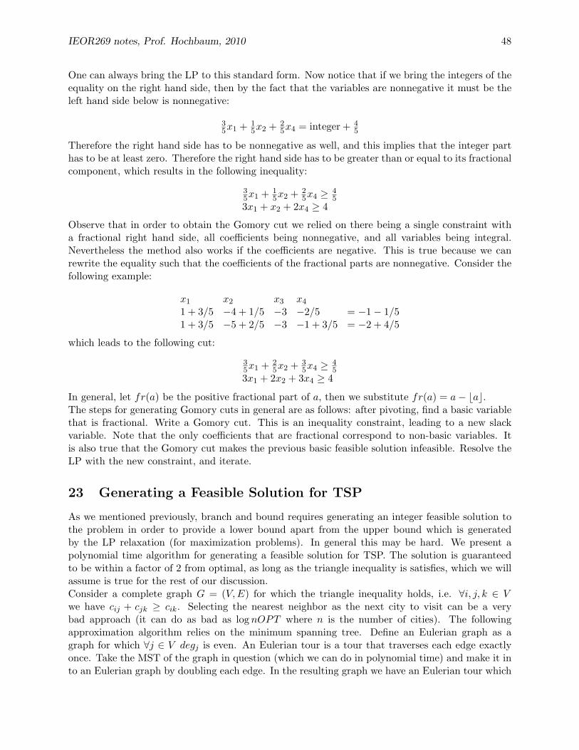
IEOR269 notes, Prof. Hochbaum, 2010 48
One can always bring the LP to this standard form. Now notice that if we bring the integers of theequality on the right hand side, then by the fact that the variables are nonnegative it must be theleft hand side below is nonnegative:
35x1 + 1
5x2 + 25x4 = integer + 4
5
Therefore the right hand side has to be nonnegative as well, and this implies that the integer parthas to be at least zero. Therefore the right hand side has to be greater than or equal to its fractionalcomponent, which results in the following inequality:
35x1 + 1
5x2 + 25x4 ≥ 4
53x1 + x2 + 2x4 ≥ 4
Observe that in order to obtain the Gomory cut we relied on there being a single constraint witha fractional right hand side, all coefficients being nonnegative, and all variables being integral.Nevertheless the method also works if the coefficients are negative. This is true because we canrewrite the equality such that the coefficients of the fractional parts are nonnegative. Consider thefollowing example:
x1 x2 x3 x4
1 + 3/5 −4 + 1/5 −3 −2/5 = −1− 1/51 + 3/5 −5 + 2/5 −3 −1 + 3/5 = −2 + 4/5
which leads to the following cut:
35x1 + 2
5x2 + 35x4 ≥ 4
53x1 + 2x2 + 3x4 ≥ 4
In general, let fr(a) be the positive fractional part of a, then we substitute fr(a) = a− bac.The steps for generating Gomory cuts in general are as follows: after pivoting, find a basic variablethat is fractional. Write a Gomory cut. This is an inequality constraint, leading to a new slackvariable. Note that the only coefficients that are fractional correspond to non-basic variables. Itis also true that the Gomory cut makes the previous basic feasible solution infeasible. Resolve theLP with the new constraint, and iterate.
23 Generating a Feasible Solution for TSP
As we mentioned previously, branch and bound requires generating an integer feasible solution tothe problem in order to provide a lower bound apart from the upper bound which is generatedby the LP relaxation (for maximization problems). In general this may be hard. We present apolynomial time algorithm for generating a feasible solution for TSP. The solution is guaranteedto be within a factor of 2 from optimal, as long as the triangle inequality is satisfies, which we willassume is true for the rest of our discussion.Consider a complete graph G = (V,E) for which the triangle inequality holds, i.e. ∀i, j, k ∈ Vwe have cij + cjk ≥ cik. Selecting the nearest neighbor as the next city to visit can be a verybad approach (it can do as bad as log nOPT where n is the number of cities). The followingapproximation algorithm relies on the minimum spanning tree. Define an Eulerian graph as agraph for which ∀j ∈ V degj is even. An Eulerian tour is a tour that traverses each edge exactlyonce. Take the MST of the graph in question (which we can do in polynomial time) and make it into an Eulerian graph by doubling each edge. In the resulting graph we have an Eulerian tour which

IEOR269 notes, Prof. Hochbaum, 2010 49
we can make into a tour by creating shortcuts. We do this by jumping over nodes which appear inthe list of edges which describe the Eulerian tour. The length of the tour we get must be within afactor of 2 of |MST | due to the triangle inequality. On the other hand, TSP opt ≥ |MST | becauseby removing one edge from the tour we get an MST which has to be at least as long as MST.Therefore we have developed an algorithm for generating a tour within a factor of 2 of TSP opt.There is also a polynomial time algorithm for generating a tour within a factor of 1.5 from optimal,which we do not present here.
24 Diophantine Equations
We will now discuss the problem of determining whether the following system of equations:
Ax = b x ∈ Zn
has a feasible solution, where we assume that the coefficients are integral. Consider the followingequality:
a1x1 + ...+ anxn = b x ∈ Zn (D)
For n = 1 the existence of a feasible solution is equivalent to the condition that ba1∈ Zn. For
n = 2 the idea is to find the greatest common divisor of a1, a2, which will function as the step sizein our system. The Euclidean algorithm is a polynomial time algorithm for calculating the gcd,which relies on the following fact: for a ≥ b > 0, a, b ∈ Z+ we have gcd(a, b) = gcd(b, r). Stop atgcd(a, 0) = a and output a as the result. Since r is at most half of a we require log a operations tocomplete the algorithm which makes the algorithm linear in the size of the input when the inputis provided in binary form.There is a useful extension of the Euclidean algorithm which keeps track of additional intermediatequantities in order to output r, p, q such that gcd(a, b) = r = pa + qb where p and q are relativelyprime and integer. The algorithm is presented below and again, without loss of generality, weassume that a ≥ b.
Intitializer−1 = a r0 = bp−1 = 1 p0 = 0q−1 = 0 q0 = 1t = 0
While rt 6= 0t← t+ 1
dt ←⌊rt−2
rt−1
⌋rt ← rt−2 − dtrt−1
pt ← pt−2 + dtpt−1
qt ← qt−2 + dtqt−1
LoopReturn r = rt−1 p = (−1)t+1pt q = (−1)tqt
Returning to a1x1 +a2x2 = b, we will use the extended Euclidean algorithm which has the same runtime as the Euclidean algorithm but in addition generates p, q ∈ Z such that gcd(a, b) = r = pa+qbwhere p, q are relatively prime. Consider the example of 10x1 + 3x2 = 7. We have gcd(10, 3) =

IEOR269 notes, Prof. Hochbaum, 2010 50
r = 10p + 3q where r = 1, p = 1, q = −3. Substitute the gcd for both a1 and a2 and obtain10x1 +3x2 = ry1 = 7, which implies y1 = 7. We can now backtrack y1 to obtain the desired feasiblesolution: x1 = py1 = 7, x2 = qy1 = −21.The same logic applies to any diophantine equation. From equation (D) above, we have r =gcd(a1, a2) = pa1 + qa2, from which we get a new equation:
ry + a3x3...+ anxn = b y ∈ Z, x ∈ Zn−2 (D′)
It can now be seen that (D) has a solution iff (D′) has a solution. One direction is obvious. Tosee the other direction, note that if (y, x3, ..., xn) is a solution for (D′) then (py, qy, x3, ..., xn) is asolution for (D). Therefore, the existence of a solution for an equation in Zn can be reduced tochecking if there is a solution to an equation for Z2.
24.1 Hermite Normal Form
Definition 24.1. An integral matrix of full rank is said to be in Hermite normal form if it has theform (H|0) where H is non-singular, lower triangular, in which |hij | ≤ hii for 1 ≤ j < i ≤ n.
Theorem 24.1. If A is an m × n integer matrix with rank(A) = m then there exists an n × nunimodular matrix C such that
1. AC = [H|0] and H is Hermite normal form
2. there exists x ∈ Zn such that Ax = b iff H−1b ∈ Zn.
Proof. Elementary unimodular column operations include the following operations:
1. Exchange columns
2. Multiply a column by −1
3. Add integer multiples of one column to another
All of these operations can be represented by a unimodular matrix, that is the matrix has a deter-minant of ±1. Thus the matrix representing multiple elementary unimodular column operationsalso has determinant of ±1.Part (1) can be proved by construction, according to the following algorithm, which converts anm×n matrix A with integral coefficients and full row rank into the form[H|0] using only elementaryunimodular column operations, where H is an m × m matrix in Hermite normal form. We firstintroduce the following operations:
A′ = Operation1(A, i, j):let r := gcd(ai,i, ai,j), pai,i + qai,j = ra′i = pai + qaj
a′j =ai,iraj +
ai,jrai
return A′ = [a1, a2, ..., ai−1, a′i, ai+1, ..., a
′j , ..., an]
A′ = Operation2(A, i):if ai,i < 0, then a′i = −aireturn A′ = [a1, a2, ..., ai−1, a
′i, ai+1, ..., an]

IEOR269 notes, Prof. Hochbaum, 2010 51
A′ = Operation3(A, i, j):
a′j = aj −⌈ai,jai,i
⌉ai
return A′ = [a1, a2, ..., aj−1, a′j , aj+1, ..., an]
The following is the Hermite normal form algorithm:H = Hermite(A)
For row i = 1, ...,mFor column j = i+ 1, ..., n
A=Operation1(A, i, j)LoopA=Operation2(A,i)For column j = 1, ..., i− 1
A=Operation3(A, i, j)Loop
LoopReturn H = A
Notice that the Hermitian matrix is constructed with a polynomial number of operations. Consider,for example:
A =[
2 6 14 7 7
], b =
[74
]Implement the algorithm in the handout to finally obtain
AC =[
1 0 0−3 5 0
]= [H|0], C =
−6 3 72 −1 −21 0 −2
.By then taking
H−1 =[
1 03/5 1/5
]we get x = C
[H−1b
0
]as a possible solution.
We will now prove part (2) of the previous theorem. In general, asking whether the Diophantineequation has a feasible solution is equivalent to asking if b ∈ L(A), where the lattice of an m × nmatrix A is defined as L(A) := y ∈ Rm : y = Ax, x ∈ Zn. The following lemma is true:
Lemma 24.1. If A is m× n, C is n× n unimodular, then L(A) = L(AC).
Proof. Let x = Cw. Then
L(A) = y ∈ Rm : y = ACw,Cw ∈ Zn= y ∈ Rm : y = ACw,w ∈ Zn= L(AC)
where the second equality follows from the fact that C is unimodular.
Therefore Ax = b has in integer solution iff ACw = b has an integer solution. This is equivalent to[H|0]w = b having an integer solution, which implies that H−1b is integer iff Ax = b has an integersolution, proving part (2).

IEOR269 notes, Prof. Hochbaum, 2010 52
Since w = H−1b, solves ACw = b, then a solution to Ax = b is x = C[H−1b
0
].
Lec7
25 Optimization with linear set of equality constraints
When the constraints are a set of linear equations over real variables (and not inequalities), opti-mization is independent of the cost function11. There can be following three cases:
1. optimal cost is unbounded: If the system of linear equations is under-constrained.
2. no feasible solution: If the system of linear equations is over-constrained and no feasiblesolution exists.
3. exactly one solution: If the system of linear equation has a unique solution.
26 Balas’s additive algorithm
Balas’s additive algorithm is a Branch and Bound algorithm that does not use LP. It considersbinary ILP in the following standard form.
minn∑j=1
cjxj
subject ton∑j=1
aijxj ≥ bi for i = 1, . . . ,m
xj ∈ 0, 1 for j = 1, . . . , n0 ≤ c1 ≤ c2 ≤ · · · ≤ cn
All the coefficients ci are non-negative and in increasing order.
Theorem 26.1. Any ILP can be reduced to the standard form above.
Proof. We give a proof by construction. The following series of transformations can reduce an ILPinto the standard form.
1. Integer variables to binary variables: Any integer variable xj can be coded in binary usingblog ujc + 1 binary variables12, where 0 ≤ xj ≤ uj . Define blog ujc + 1 new variables, suchthat
xj =blog ujc∑k=0
2kxkj
If the ILP has a finite optimal feasible solution, we can compute the upper bound of eachcomponent (uj) as a polynomial function of the input (Theorem 13.5 in [21]).
11If the cost function is∑i aixi and the linear equation is
∑i aixi = d, then the optimal cost is d
120 ≤ uj ≤ 2n − 1 can be expressed using n bits. So, n ≥ log (uj + 1)

IEOR269 notes, Prof. Hochbaum, 2010 53
2. Optimization Objective: If the optimization objective is to maximize some linear expressioncjxj , that is,
OPT = maxn∑j=1
cjxj
we rewrite it as a minimization problem by defining the objective
OPT ′ = min (−n∑j=1
cjxj)
The optimum for the maximization problem can be obtained from the computed optimumfor the minimization problem as OPT = −OPT ′. Hence, we can reduce any optimizationproblem with maximization objective to one with minimization objective.
3. All constraints as ≥ constraints:
• if there is an equality, we replace it with two constraints ≤ and ≥.
• if the inequality is ≤ , multiply the inequality by −1 to get it in the desired ≥ form.
• Write all constraints as ≥ constraints with the RHS of the inequalities being just theconstant term.
4. Positive costs: All coefficients in the objective function must be positive. So, if a variable xhas a negative coefficient in the objective function, then we must make a ‘change of variable’,say to a (binary) variable y, such that y = 1 − x. We need to change all occurrences of thevariable x with 1− y in our problem formulation (this includes both: the objective functionand the constraints).
5. Ordered costs: Change the indices of the variables so that the indices are ordered accordingto monotone non-decreasing coefficients. Ties can be broken arbitrarily. The coefficients withnew indices would be ordered in an increasing order, that is,
c1 ≤ c2 ≤ · · · ≤ cn
Steps of the Algorithm
1. Initialization:
(a) Check the problem for infeasibility. If the problem is infeasible then stop.
(b) Set the lower bound to zero and the upper bound to ∞.
2. Branch on the node with the smallest lower bound, and in the order of increasing index ofthe variables.
3. If a 0-completion is feasible, then we have found a feasible solution to our sub-problem. Inparticular, if this feasible solution is the best one found so far, then update the upper boundto its optimal value.
4. • When the most recent variable was fixed to 1, and a 0-completion is not feasible, thenthe value of the optimization objective at the node is a lower bound.

IEOR269 notes, Prof. Hochbaum, 2010 54
• When the most recent variable was fixed to 0, and a 0-completion is not feasible, thenthe lower bound for such a node is obtained by setting the next unfixed variable to beequal to one13.
5. Check the new sub-problem for infeasibility.
6. As in the general branch and bound algorithm for minimization, we fathom a node if:
• it has a feasible solution
• the problem is infeasible
• the lower bound of the current node is higher than the current upper bound
7. Keep branching until all nodes are fathomed.
Illustrative Example
Let us consider the following ILP problem.
min Z = 3x1 + 5x2 + 6x3 + 9x4 + 10x5 + 10x6
subject to −2x1 + 6x2 − 3x3 + 4x4 + x5 − 2x6 ≥ +2−5x1 − 3x2 + x3 + 3x4 − 2x5 + x6 ≥ −25x1 − x2 + 4x3 − 2x4 + 2x5 − x6 ≥ +3xj ∈ 0, 1 for j = 1, 2, . . . , 6
In Figure 18, we illustrate how Balas’ Additive Method work works by showing two intermediatesteps for the above ILP problem. After step 4, the node with the least lower bound of the objectivefunction is the node with x1 = 0. The lower bound for this node is 5. We branch on x2 setting x2
as 1 in step 5. The lower bound of the objective function is again 5. At this point, there are twonodes with the same lower bound. We choose the node with smaller index variable. We branchon x2 again setting x2 as 0 in step 6. The lower bound for this node is 6. Now, the best node tobranch would be the one with x2 = 1. The lower bound of objective function is 5 at this node.Since the next index is 3, we would branch on x3.
13As noted in class, this can also be done when the most recent variable was fixed to 1, and the 0-completion isnot feasible. In Balas’ additive algorithm however, this improvement on the bound was used only when the recentvariable to be fixed was set to 0.

IEOR269 notes, Prof. Hochbaum, 2010 55
0
1
All
3
5
0
9
Step 1
Step 2
Step 3
1
8
Step 4
x1
x2
(a) Step 1 to 4
0
1
All
3
5
0
9
Step 1
Step 2
Step 3
1
8
Step 4
0
1
6
5
Step 5
Step 6
x1
x2
(b) Step 5 and 6
Figure 18: Balas’ Additive Method Example
27 Held and Karp’s algorithm for TSP
One way of formulating the TSP problem on a graph G = (V,E), where V = 1, 2, . . . , n is aset of nodes and E is the set of edges, is to consider an 1-tree. An 1-tree is a spanning tree overV \ 1 nodes + 2 edges adjacent to node 1. 1-tree with least cost can be computed by findingthe minimum spanning tree and then adding the cheapest edges adjacent to node 1. So, cost of anoptimal 1-tree T ∗ is at-most the cost of the optimal tour TSP ∗.
| T ∗ |≤| TSP ∗ |
Proof sketch: Consider an optimal tour. Remove edges adjacent to node 1. The remaining edgesof the tour form a spanning tree of nodes i = 2, . . . , n. The cost of this spanning tree is greaterthan or equal to the cost of the minimum spanning tree. Optimal 1-tree is obtained by adding 2cheapest edge adjacent to node 1. Thus, the cost of the optimal tour is greater than or equal tothe cost of the 1-tree.
An important observation:
The following constraints suffice to enforce that every node is of degree 2.∑j>i
xij +∑j<i
xji = 2, i = 1, . . . , n− 1
∑1≤i<j≤n
xij = n
The first constraint ensures that all nodes i = 1, . . . , n − 1 are of degree 2. There is no need tospecify that node n is of degree 2 because of the following lemma from graph theory:
Given a graph with nodes of degrees d1, d2, . . . , dn, then, m = |E| =∑n
i=1 di/2.
Problem of finding minimum weight 1-tree:
This problem is solvable in polynomial time. We describe the two-step method below:

IEOR269 notes, Prof. Hochbaum, 2010 56
1. Find MST on 2, . . . , n. Greedy methods for MST give optimal answer and run in polyno-mial time (O(m log n)). Some examples are Prim’s algorithm for MST [23]14 and Kruskal’salgorithm [16]
2. Add 2 cheapest edges adjacent to 1. The two cheapest edges can be found by a linear passover all the neighbors of node 1. The neighbors can be atmost n − 1. So, the complexity ofthis step is (O(n)).
Complexity: So, the overall complexity of finding optimum 1-tree is O(m log n)In order to guarantee that the computed 1-tree is a tour, we require that there is no cycle in2, . . . , n (subtour elimination).
Subtour elimination to transform a 1-tree to a tour:
The following ILP formulation uses the idea of 1-tree with no cycles in nodes i = 2, . . . , n tofind an optimal TSP.
min∑
1≤i<j≤ncijxij
subject to∑j>i
xij +∑j<i
xji = 2 for i = 2, . . . , n− 1
∑i<j,i,j∈S
xij ≤ |S| − 1 for S ⊂ 2, . . . , n
∑j
x1j = 2
∑1≤i<j≤n
xij = n,
xij ∈ 0, 1 for i < j
Note: Constraint∑
i<j,i,j∈S xij ≤ |S| − 1 is added for all S ⊂ 2, . . . , n. So, the number of con-straints in this formulation is exponential in the number of nodes.
28 Lagrangian Relaxation
This is based on relaxing constraint the constraint∑j>i
xij +∑j<i
xji = 2 for i = 2, . . . , n− 1
which imposes the restriction that the degree of each node is exactly 2.
L(~π) =∑
1≤i<j≤ncijxij +
n−1∑i=2
πi(2− [∑j>i
xij +∑j<i
xji])
where πi unrestricted and∑
j>i xij +∑
j<i xji = di, the degree of node i.
14Complexity depends on data structures used. The best is O(m log n).

IEOR269 notes, Prof. Hochbaum, 2010 57
Consider the following integer program,
min L(~π)
subject to∑
i<j,i,j∈Sxij ≤ |S| − 1 for S ⊂ 2, . . . , n
∑j
x1j = 2
∑1≤i<j≤n
xij = n,
xij ∈ 0, 1 for i < j
We can rewrite L(~π) as:
L(~π) =∑
1≤i<j≤ncijxij − 2
n−1∑i=2
πi −n−1∑i=2
πidi
that is,
L(~π) = 2n−1∑i=2
πi +∑
1≤i<j≤n(cij − πi − πj)xij
Let L∗ = min L(~π) and TSP ∗ be the cost of the optimal tour. We know that
|L∗| ≤ |TSP ∗|
An Illustrative Example:
The example is presented in Figure 19.
1
5
1
4
5
53
7
2
8
5
F
AD
B
C E
G
2
Figure 19: Example for Lagrangian Relaxation

IEOR269 notes, Prof. Hochbaum, 2010 58
We assume that edges not present have cost = 20. One tour found by inspection, with total weight28, is: GDBAFCEG
Let node 1 = G. We compute the minimum spanning tree for nodes A− F and add the edges DGand EG to it to form the 1-tree. The found 1-tree is illustrated in Figure 20.
1
1
4
2
8
5
F
AD
B
C E
G
2
Figure 20: 1-Tree with L((A,B,C,D,E, F ) = (0, 0, 0, 0, 0, 0))
The cost for this 1-tree is 21
L((A,B,C,D,E, F ) = (0, 0, 0, 0, 0)) = 21
L(~π∗) = min~π
L(~π)
The search for ~π∗ is done using the sub-gradient method. For i = 2, . . . , n,
• if∑
j xij < 2, πi is increased, that is, πi
• if∑
j xij > 2, πi is decreased, that is, πi
Given, the solution for L((A,B,C,D,E, F ) = (0, 0, 0, 0, 0, 0)), we make the following changes:
• πB , πC , πE , πF
• πA, πD remain unchanged.
The graph obtained after revision of the weights is illustrated in Figure 21. The 1-tree obtained isillustrated in Figure 22. The cost for this 1-tree is 23.
L((A,B,C,D,E, F ) = (0,−1, 1, 0,−1, 1)) = 23 + (0 + (−1) + 3(−1) + 0 + 3(−1) + 2(1)) = 24
Given, the computed tree for L((A,B,C,D,E, F ) = (0,−1, 1, 0,−1, 1)), we can make the followingchanges:
• πA , πB , πC , πE
• πD, πF remain unchanged.
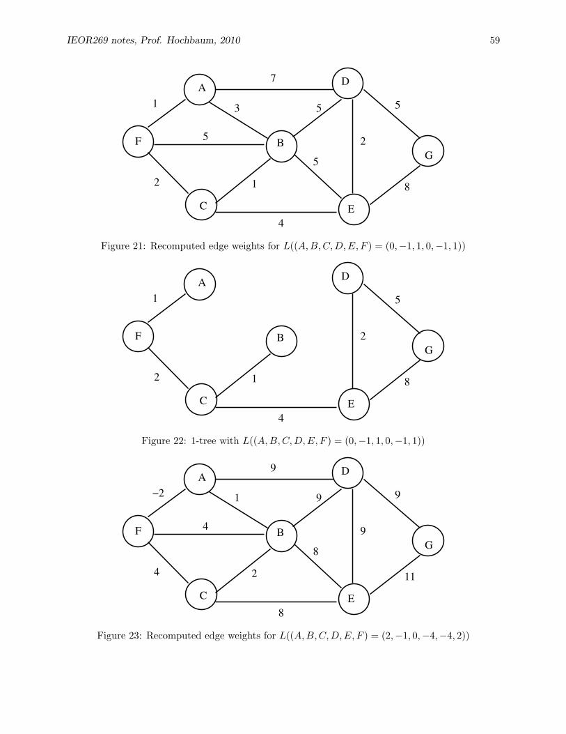
IEOR269 notes, Prof. Hochbaum, 2010 59
1
5
1
4
5
53
7
2
8
5
F
AD
B
C E
G
2
Figure 21: Recomputed edge weights for L((A,B,C,D,E, F ) = (0,−1, 1, 0,−1, 1))
1
1
4
2
8
5
F
AD
B
C E
G
2
Figure 22: 1-tree with L((A,B,C,D,E, F ) = (0,−1, 1, 0,−1, 1))
F
AD
B
C E
G
4
−21
24
9
9 9
9
11
8
8
Figure 23: Recomputed edge weights for L((A,B,C,D,E, F ) = (2,−1, 0,−4,−4, 2))

IEOR269 notes, Prof. Hochbaum, 2010 60
F
AD
B
C E
G
−21 9 9
11
8
2
Figure 24: 1-tree with L((A,B,C,D,E, F ) = (2,−1, 0,−4,−4, 2))
Let us consider the following set of multipliers.
πA = 2, πB = −1, πC = 0, πD = −4, πE = −4, πF = 2
Revising the costs revises the weight of the edges and the problem reduces to finding 1-tree of thegraph illustrated in Figure 23. The 1-tree obtained is illustrated in Figure 24. The cost for this1-tree is 38.
L((A,B,C,D,E, F ) = (2,−1, 0,−4,−4, 2)) = 38 + 2(2 + (−1) + 0 + (−4) + (−4) + 2) = 28
The obtained 1-tree is also a tour and is in fact, an optimal tour. So, we find the cost of the mostoptimal tour in this example to be 28 and a tour with this cost is GDBAFCEG. Lec8
29 Lagrangian Relaxation
One of the most computationally useful ideas of the 1970’s is the observation that many hardproblems can be viewed as easy problems complicated by a relatively small set of side constraints.Define the problem
max cx
subject to Ax ≤ bCx ≤ dx ≥ 0, integer
We relax the set of constraints Ax ≤ b and add them to the objective function as a ’penalty term’to obtain the following problem, L(λ)
L(λ)λ≥0 = max cx+ λ(b−Ax) = (c− λA)x+ λb (13)subject to Cx ≤ d
x ≥ 0, integer
We restrict the λ’s to be positive to add a penalty when the constraint Ax ≤ b is not satisfied. IfAx ≤ b is changed to Ax ≥ b then we restrict the λ’s to be negative. If the constraint is Ax = b

IEOR269 notes, Prof. Hochbaum, 2010 61
then the λ’s are unrestricted.
We have the following relationship between L(λ) and Z;
Theorem 29.1. L(λ) ≥ Z
Proof. Let x∗ be the optimal solution for (1). Then we have that x∗ is also a feasible solution toL(λ). Therefore, L(λ) is an upper bound for Z.
We would like the lowest upper bound on Z so we find the minimum of L(λ) over all λ ≥ 0.
ZD = minλ≥0
L(λ) (14)
In the case of one variable, this problem can easily be seen to be a piecewise linear convex functionof a single variable. However, it is not easy to see for larger dimensions, so we prove the following.
Theorem 29.2. L(λ) is convex.
Proof. Let λ ≥ 0 and λ = θλ1 + (1− θ)λ2 for 0 ≤ θ ≤ 1 and λ1, λ2 ≥ 0. Also, let x be an optimalsolution to L(λ), and X = x ∈ Z|Dx ≤ e, x ≥ 0
L(λ) = maxx∈X
cx+∑i
λi(b−Aix)
= cx+∑i
λi(b−Aix)
Since x is the optimal solution for λ, x is not necessarily optimal for λ1 or λ2. So we have thefollowing inequalities,
L(λ1) ≥ cx+∑i
λ1i (b−Aix)
L(λ2) ≥ cx+∑i
λ2i (b−Aix)
Therefore,
θL(λ1) + (1− θ)L(θ2) ≥ L(θλ1 + (1− θ)λ2)
To solve (2), one such method is the steepest descent algorithm. To begin this algorithm, choose astarting lambda, λ0
L(λ0) = maxx∈X
cx+ λ0(b−Ax)
We solve this problem and denote the optimal solution by x0. We now want to update λ0. Thesteepest descent method chooses the negative of the gradient of the objective function of (2) asthe direction of descent. Hence, we take the gradient of cx0 + λ(b− Ax0) with respect to λ. Thisgradient is easily seen to be (b − Ax0). We update the λ’s using the following relation (where weare now updating from λi−1 to λi):
λi = λi−1 − [(b−Axi−1)||b−Axi−1||
]si−1

IEOR269 notes, Prof. Hochbaum, 2010 62
Where si−1 is the step size at the ith iteration.
For the steepest descent algorithm to converge, the step sizes must satisfy the following sufficientconditions (although they are typically not the fastest for converging, e.g. sk = 1
k ),
∞∑k=1
sk =∞
limk→∞
sk = 0
However, Fisher recommends the following step sizes,
sk =λk(L(λk)− Z∗)∑
i(bi −Aixki )2
Where Z∗ is the value of the best feasible solution found so far. Note, if L(λk) = Z∗ then, byTheorem 1.1, we have found a feasible solution that is also optimal. This will cause the next stepsize to be zero in Fisher’s formula, which is an indication that we are at the optimal solution.Therefore, the algorithm terminates when we have indeed found an optimal feasible solution.
In Practice, Lagrangian Relaxation is typically done in the following manner:1.) Choose a subset of constraints to relax (typically the constraints that makes the resulting prob-lem easier to solve).2.) Solve the sub problem with the relaxed constraints.3.) Find a proper step size (e.g. Fisher’s) and solve using Steepest Descent or another algorithm.
30 Complexity of Nonlinear Optimization
30.1 Input for a Polynomial Function
To input a function that is a polynomial of the form a0 + a1x + a2x2 + . . . + akx
k, we form a(k + 1) × 1 vector whose entries are the k + 1 coefficients of the polynomial. The ith entry of thevector is ai−1.For a polynomial with two variables, we form a two dimensional matrix with the ijth entry equalto aij where aij is the coefficient of the term xi−1yj−1 (i.e. aijxi−1yj−1). The resulting matrix willbe k1 + 1× k2 + 1, where k1 is the highest exponent of x and k2 is the highest exponent of y.For polynomials with more variables, we follow the same method by using a matrix with the samedimensions as the number of variables.Note, only polynomial functions can be represented with this method. For a general non-linearfunction, we do not have a good representation for input.
30.2 Table Look-Up
When working with computers, we restrict the accuracy of the numbers we are working with sincewe can only compute with finite precision.Even though there is no nice representation for general non-linear functions, we can use a methodcalled Table Look-Up during the execution of an algorithm. If we have a function of severalvariables, f(x1, . . . , xn), table look-up takes an argument that is a vector, x ∈ Rn, and delivers the

IEOR269 notes, Prof. Hochbaum, 2010 63
value of the function at x, f(x), with specified accuracy. Table look-up can be visualized in thefollowing table format,
x f(x)...
...
30.3 Examples of Non-linear Optimization Problems
When dealing with non-linear optimization problems there are two alternative characterizations ofoptimal solutions,
|f(x)− f(x∗)| ≤ ε (15)||x− x∗|| ≤ ε (16)
(3) indicates that x is an ε-approximate solution, where x∗ is the optimal solution. (4) indicatesthat x is an ε-accurate solution, where x∗ is the optimal solution as well. Note: for an ε-approximatesolution, the values of x that satisfy this inequality could be arbitrarily far from the optimal solu-tion, x∗. Also note: for an ε-accurate solution, the value of the function at values of x that satisfythis inequality could be arbitrarily far from the value of the function at the optimal solution, f(x∗).
An example that involves separable convex optimization over linear constraints is,
minn∑j=1
fj(xj)
subject to Ax = b (17)l ≤ x ≤ u
where the fj ’s are convex functions ∀j.Note: A problem of the form P = min f(x) : x ∈ Rn cannot be addressed with finite complexity.This is because we are dealing with real numbers, which we cannot represent. We can only use arational approximation which limits the accuracy of the numbers in our computations.
A problem in the form of (5), is the following optimization problem with piecewise linear functions.In the new problem the fj(x)’s are piecewise linear functions with k-pieces (i.e. the function fj ismade up of k linear pieces):
minn∑j=1
fj(xj)
subject to Ax = b (18)x ≥ 0
We transform problem (6) into the following:
minn∑j=1
b0,j +k∑i=1
cijδij
subject ton∑j=1
Aj(k∑i=1
δij) = b
dij ≥ δij ≥ 0, ∀i ∈ 1, . . . , k, j ∈ 1, . . . , n

IEOR269 notes, Prof. Hochbaum, 2010 64
f (x)ij
s
f (x)ij
x
Figure 25: Linear Piecewise Approximation
Where dij is the length of the ith linear piece of the jth function; Aj is the jth column of A; δijis the length of the ith linear piece of the jth function that is actually used; xj =
∑ki=1 δij ; b0,j
is the value fj(0) function; and cij is the slope of the ith linear piece of the jth function. Noticethat we can get rid of the constant term in the objective function since this term will not effectthe minimization. Also note that we do not need to enforce the requirement that if δij > 0 thenδi−1,j = di−1,j . This is because since we are dealing with a convex function, the slopes (cij ’s) areincreasing. Hence, the minimization will force the δij ’s corresponding to the lower cij ’s to reach dijbefore the next one becomes non-zero.
The following theorem, stated without proof, is known as the Proximity Theorem. The s-piecewiselinear optimization problem mentioned in the theorem is problem (6) with each segment havinglength s.
Theorem 30.1. Let x∗ ∈ Rn be the optimal solution vector to problem (6), and xs ∈ Rn be theoptimal solution to the s-piecewise linear optimization problem, where s is the length of each linearpiece segment. Then ||x∗ − xs||∞ ≤ n∆s where ∆ is the maximum sub-determinant of A.
From the above theorem, we see that in order to have an ε-accurate solution to problem (6) weneed n∆s ≤ ε. Therefore, if s ≤ ε
n∆ , then xs will indeed be an ε-accurate solution to problem (6)(i.e. ε ≥ n∆s). We can subdivide the interval [`, u] into 4n∆ pieces.
u− `4n∆
= s
Notice, the length of each linear piece depends on the sub-determinant of A. This value, ∆ takes apolynomial number of operations to compute. Substituting ∆ pieces makes the number of variables

IEOR269 notes, Prof. Hochbaum, 2010 65
pseudopolynomial.Instead, we can iteratively divide the interval u − ` into halves until we get the length of eachlinear piece that will yield an ε-accurate solution. More precisely, the Proximity-Scaling Algorithm(Hochbaum and Shantikumar):
The proximity-scaling algorithm can be employed whenever there is a valid proximity theorem. Forconvex network flow the proximity theorem is ||xs − x
s2 ||∞ ≤ ms. We call α the proximity factor
(In our case, α = n∆) if ‖ xs − xs2 ‖∞≤ αs.
The algorithm is implemented as follows. The scaling unit is selected initially to be s = d U4αe forU = max(i,j)∈Auij − `ij. The interval for variable xij , [`ij , uij ] is thus replaced by up to 4αintervals of length s each.
Proximity-scaling algorithm:
Step 0: Let s = d U4αe.
Step 1: Solve (LNF-s) or (INF-s) with an optimal solution xs. If s = 1 output the solution and stop.
Step 2: Set `ij ← max`ij , xsij − αs and uij ← minuij , xsij + αs, for (i, j) ∈ A.
Step 3: s← d s2e. Go to step 1.
The total number of iterations will be,
(12
)q(u− `) ≤ ε
u− `ε≤ 2q
d(log2
U
ε)e = q
Where U = u− `
30.4 Impossibility of strongly polynomial algorithms for nonlinear (non-quadratic)optimization
Consider the Allocation Problem, where the fj(x)’s are piecewise linear functions with k-pieces:
maxn∑j=1
fj(xj)
subject ton∑j=1
xj ≤ B
uj ≥ xj ≥ 0
To solve this problem we perform a Greedy Algorithm by calculating the gradients (i.e. ∆1(1),∆1(2), . . . ,∆1(k)for f1(); ∆2(1),∆2(2), . . .∆2(k) for f2(); . . . ; ∆n(1),∆n(2), . . . ,∆n(k) for fn()), where (letting dijdenote the length of the ith linear piece of the jth function)
∆j(i) =fj(∑i
l=0 dij)− fj(∑i−1
l=0 dij)dij
.

IEOR269 notes, Prof. Hochbaum, 2010 66
After we calculate the gradients, we add the highest gradients using the procedure below until werun out of capacity (i.e. we reach B).
(1) Take the largest gradient, say ∆j(i).(2) Update xj ← xj + mindij , B, uj.(2′) Temporarily store B for step (4). B ← B.(3) Update B ← [B −mindij , B, uj]. If B = 0, STOP. We have reached the optimal solution.(4) Update uj ← [uj −mindij , B, uj].(5) Delete ∆j(i). If there are remaining gradients, return to Step (1). Else, STOP.
This greedy algorithm works because the coefficient of each xj is one, so only the gradients need tobe considered when determining optimality. Any algorithm solving the simple allocation problemfor fj nonlinear and non-quadratic must depend on log2B
Please refer to the handout ”The General Network Flow Problem,” for the example explained inthe rest of class. Lec9
31 The General Network Flow Problem Setup
A common scenario of a network-flow problem arising in industrial logistics concerns the distributionof a single homogenous product from plants (origins) to consumer markets (destinations). The totalnumber of units produced at each plant and the total number of units required at each market areassumed to be known. The product need not be sent directly from source to destination, but maybe routed through intermediary points reflecting warehouses or distribution centers. Further, theremay be capacity restrictions that limit some of the shipping links. The objective is to minimize thevariable cost of producing and shipping the products to meet the consumer demand.The sources, destinations, and intermediate points are collectively called nodes of the network, andthe transportation links connecting nodes are termed arcs. Although a production/distributionproblem has been given as the motivating scenario, there are many other applications of the generalmodel. Figure 31 indicates a few of the many possible alternatives.
Table 1: Other applications
Urban Transportation Communication System Water ResourcesProduct Buses, autos, etc. Messages Water
NodesBus stops, Communication centers, Lakes, reservoirs,
street intersections relay stations pumping stationsArc Streets (lanes) Communication channels Pipelines, canals, rivers
Here is a general instance statement of the minimum-cost flow problem: Given a network G =(N,A), with a cost cij , upper bound uij , and lower bound lij associated with each directed arc(i, j), and supply bv at each node. Find the cheapest integer valued flow such that it satisfies:1) the capacity constraints on the arcs, 2) the supplies/demands at the nodes, 3) that the flow isconserved through the network.
A numerical example of a network-flow problem is given in Figure 26. The nodes are represented bynumbered circles and the arcs by arrows. The arcs are assumed to be directed so that, for instance,

IEOR269 notes, Prof. Hochbaum, 2010 67
material can be sent from node 1 to node 2, but not from node 2 to node 1. Generic arcs willbe denoted by (i, j), so that (4, 5) means the arc from 5 to 5. Note that some pairs of nodes, forexample 1 and 5, are not connected directly by an arc.
!"
#"
$"
%"
&"
(15,$4)
(!,$2)
(8,$4)
(4,$2)
(10,$6) (15,$1)
(4,$1)
(!,$2)
(5,$3)
Figure 26: Numerical example of a network-flow problem
Figure 26 exhibits several additional characteristics of network flow problems. First, a flow capacity(uij) is assigned to each arc (i,j), and second, a per-unit cost (cij) is specified for shipping alongeach arc (i,j). There characteristics are shown next to each arc. This, the flow on arc 2-4 must bebetween 0 and 4 units, and each unit flow on this arc costs $2.00. The ∞’s in the figure have beenused to denote unlimited flow capacity on arcs (2, 3) and (4, 5). Finally, the numbers in parenthesisnext to the nodes give the material supplied or demanded (bi) at that node i. In this case, node1 is an origin or source node supplying 20 units, and nodes 4 and 5 are destinations or sink nodesrequiring 5 and 15 units, respectively, as indicated by the negative signs. The remaining nodes haveno net supply or demand; they are intermediate points, often referred to as transshipment nodes.
The objective is to find the minimum-cost flow pattern to fulfil demands from the source nodes.such problems usually are referred to as minimum-cost flow or capacitated transhipment problems.To transcribe the problem into a formal linear program, let
fij = feasible flow = Number of units shipped from node i, to j using arc (i, j).
Then the tabular form of the linear-programming formulation associated with the network of Fig-ure 26 is as shown in Figure 31.
The first five equations are flow-balance equations at the nodes. They state the conservation-of-flowlaw,The distinctive feature of this matrix of the flow balance constraint matrix is that each column hasprecisely one 1 and one −1 in it.
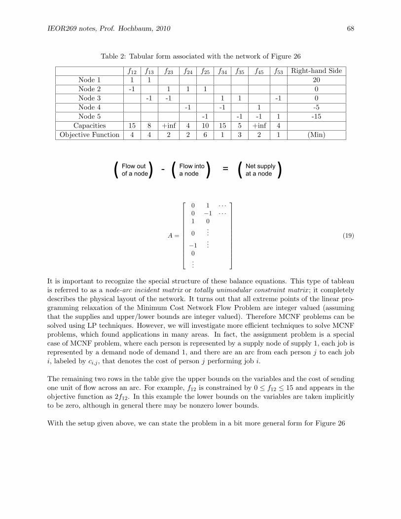
IEOR269 notes, Prof. Hochbaum, 2010 68
Table 2: Tabular form associated with the network of Figure 26
f12 f13 f23 f24 f25 f34 f35 f45 f53 Right-hand SideNode 1 1 1 20Node 2 -1 1 1 1 0Node 3 -1 -1 1 1 -1 0Node 4 -1 -1 1 -5Node 5 -1 -1 -1 1 -15
Capacities 15 8 +inf 4 10 15 5 +inf 4Objective Function 4 4 2 2 6 1 3 2 1 (Min)
Flow out of a node
Flow into a node
Net supply at a node ( ( ( ) ) ) = -
A =
0 1 · · ·0 −1 · · ·1 0
0...
−1...
0...
(19)
It is important to recognize the special structure of these balance equations. This type of tableauis referred to as a node-arc incident matrix or totally unimodular constraint matrix ; it completelydescribes the physical layout of the network. It turns out that all extreme points of the linear pro-gramming relaxation of the Minimum Cost Network Flow Problem are integer valued (assumingthat the supplies and upper/lower bounds are integer valued). Therefore MCNF problems can besolved using LP techniques. However, we will investigate more efficient techniques to solve MCNFproblems, which found applications in many areas. In fact, the assignment problem is a specialcase of MCNF problem, where each person is represented by a supply node of supply 1, each job isrepresented by a demand node of demand 1, and there are an arc from each person j to each jobi, labeled by ci,j , that denotes the cost of person j performing job i.
The remaining two rows in the table give the upper bounds on the variables and the cost of sendingone unit of flow across an arc. For example, f12 is constrained by 0 ≤ f12 ≤ 15 and appears in theobjective function as 2f12. In this example the lower bounds on the variables are taken implicitlyto be zero, although in general there may be nonzero lower bounds.
With the setup given above, we can state the problem in a bit more general form for Figure 26

IEOR269 notes, Prof. Hochbaum, 2010 69
min∑
(i,j)∈A
cijfij
subject to (f23 + f25 + f24)− f12 = 0 (20)(f35 + f34)− (f13 + f23 + f53) = 0 (21)f45 − (f24 + f34) = −5 (22)f53 − (f25 + f35 + f45) = −15 (23)0 ≤ fij ≤ Uij ∀(i,j)∈A (24)
To further generalize a Minimum-cost Flow Problem with n nodes, we have the following formula-tion:
min z =∑i
∑j
cijfij
subject to∑j
fij −∑k
fki = bi ∀i=1,2,...,n [Flow Balance] (25)
lij ≤ fij ≤ uij [Flow Capacities] (26)
Comments: The first set of constraints is formed by the flow balance constraints. The second setis formed by the the capacity constraints. Nodes with negative supply are sometimes referred to asdemand nodes and nodes with 0 supply are sometimes referred to as transshipment nodes. Noticethat the constraints are dependent (left hand sides add to 0, so that the right hand sides must addto for consistency) and, as before, one of the constraints can be removed. Another thing that worththinking is that what would happen if we have a negative cost on an arc. For example, let C35 = 3and C53 = −6, we will then have a negative cycle in our network. Therefore we could just use thiscycle repeatedly to minimize our total cost. Hence our problem becomes unbounded. Hence weconclude that as long as we don’t have a negative cycle in our network, we are then ok with havingnegative costs on our arc(s).
32 Shortest Path Problem
The Shortest Path problem is defined on a directed, weighted graph, where the weights may bethought of as distances. The objective is to find a path from a source node, s, to node a sink node,t, that minimizes the sum of weights along the path. To formulate as a network flow problem, letxi,j be 1 if the arc (i, j) is in the path and 0 otherwise. Place a supply of one unit at s and ademand of one unit at t. The formulation for the problem is:

IEOR269 notes, Prof. Hochbaum, 2010 70
min∑
((i,j)∈A
di,jxi,j
subject to∑
(i,k)∈A
xi,k −∑
(j,i)∈A
xj,i = 0 ∀i 6= s, t (27)
∑(s,i)∈A
xs,i = 1 (28)
∑(j,t)∈A
xj,t = 1 (29)
0 ≤ xi,j ≤ 1 (30)
This problem is often solved using a variety of search and labeling algorithms depending on thestructure of the graph.
33 Maximum Flow Problem
33.1 Setup
The Maximum Flow problem is defined on a directed network G = (V,A) with capacities uij onthe arcs, and no costs. In addition two nodes are specified, a source node, s, and sink node, t. Theobjective is to find the maximum flow possible between the source and sink while satisfying the arccapacities. (We assume for now that all lower bounds are 0.)
Definitions:• A feasible flow f is a flow that satisfied the flow-balance and capacity constraints.• A cut is a partition of the nodes (S, T ), such that S ⊆ V , s ∈ S, T = V \ S, t ∈ T .• Cut capacity: U(S, T ) =
∑i∈S∑
j∈T uij . (Important: note that the arcs in the cut areonly those that go from S to T .)
An Example
5
1
2
3
4
6
5(5)
4(4)
7(5)
1(1)
5(4)
4(4)
1(1)
4(3)
8(8)
6(6)
Figure 27: Maximum Flow Setup Example
See Figure 27, on each arc, we have a capacity and the amount of actual flow(within the paren-thesis). The source node in the graph is node 5 and the sink node is in the graph is node 6. The

IEOR269 notes, Prof. Hochbaum, 2010 71
current solution is optimal; next, we will find a certificate of optimality.
Intuition:Find a Minimum Cut.A cut is said to be a minimum cut if it has the minimum cut capacity.In this particular example, we can tell that node 2 and node 5 form a minimum cut (i.e. minimal source set),that is a source set S. We can also find that node 1, 3, 4 and 6 form a sink set T. Since from anynode (2 and 5) in the source set, we can’t send any flow to T (all the capacities of the arcs comingout of this cut has been used). For the same reasoning, we can also tell that node 1, node 3, node4 and node 6 form a minimum cut (i.e. maximal sink set).
Claim:Given a maximum flow, we can always find a minimum cut (with minimal source set or with max-imal source set)
Clarification: What is the difference between maximum and maximal?An example of maximum/maximal independence set (IS):See Figure 28 A maximum IS (node 1, 3and 5) is a largest independent set for a given graph G(i.e. maximum independence)A maximal IS (node 2 and 5) is an independent set that is not a subset of any other independentset (i.e. we can’t add or remove any nodes from the set to maintain its independence).
1
2
3
4
5
Maximal Independent Set
Maximum Independent Set
Figure 28: Maximum Independent Set Example
Let |f | be the total amount of flow out of the source (equivalently into the sink). It is easy toobserve that any feasible flow satisfies
|f | ≤ U(S, T ) (31)
for any (S, T ) cut. This is true since all flow goes from s to t, and since s ∈ S and t ∈ T (bydefinition of a cut), then all the flow must go through the arcs in the (S, T ) cut. Inequality 31 is aspecial case of the weak duality theorem of linear programming.

IEOR269 notes, Prof. Hochbaum, 2010 72
The following theorem, which we will establish algorithmically, can be viewed as a special case ofthe strong duality theorem in linear programming.
Theorem 33.1 (Max-Flow Min-Cut). The value of a maximum flow is equal to the capacity of acut with minimum capacity among all cuts. That is,
max |f | = minU(S, T )
33.2 Algorithms
Next we introduce the terminology needed to prove the Max-flow/Min-cut duality and to give usan algorithm to find the max flow of any given graph.
Residual graph: The residual graph, Gf = (V,Af ), with respect to a flow f , has the followingarcs:• forward arcs: (i, j) ∈ Af if (i, j) ∈ A and fij < uij . The residual capacity is ufij = uij − fij .
The residual capacity on the forward arc tells us how much we can increase flow on the originalarc (i, j) ∈ A.• reverse arcs: (j, i) ∈ Af if (i, j) ∈ A and fij > 0. The residual capacity is ufji = fij . The
residual capacity on the reverse arc tells us how much we can decrease flow on the originalarc (i, j) ∈ A.
Intuitively, residual graph tells us how much additional flow can be sent through the originalgraph with respect to the given flow. This brings us to the notion of an augmenting path. Inthe presence of lower bounds, `ij ≤ fij ≤ uij , (i, j) ∈ A, the definition of forward arc remains,whereas for reverse arc, (j, i) ∈ Af if (i, j) ∈ A and fij > `ij . The residual capacity is ufji = fij−`ij .
Augmenting path: An augmenting path is a path from s to t in the residual graph. The capacityof an augmenting path is the minimum residual capacity of the arcs on the path – the bottleneckcapacity.If we can find an augmenting path with capacity δ in the residual graph, we can increase the flowin the original graph by adding δ units of flow on the arcs in the original graph which correspondto forward arcs in the augmenting path and subtracting δ units of flow on the arcs in the originalgraph which correspond to reverse arcs in the augmenting path.Note that this operation does not violate the capacity constraints since δ is the smallest arccapacity in the augmenting path in the residual graph, which means that we can always add δunits of flow on the arcs in the original graph which correspond to forward arcs in the augmentingpath and subtract δ units of flow on the arcs in the original graph which correspond to reverse arcsin the augmenting path without violating capacity constraints.The flow balance constraints are not violated either, since for every node on the augmenting pathin the original graph we either increment the flow by δ on one of the incoming arcs and incrementthe flow by δ on one of the outgoing arcs (this is the case when the incremental flow in the residualgraph is along forward arcs) or we increment the flow by δ on one of the incoming arcs and decreasethe flow by δ on some other incoming arc (this is the case when the incremental flow in the residualgraph comes into the node through the forward arc and leaves the node through the reverse arc)or we decrease the flow on one of the incoming arcs and one of the outgoing arcs in the originalgraph (which corresponds to sending flow along the reverse arcs in the residual graph).

IEOR269 notes, Prof. Hochbaum, 2010 73
33.2.1 Ford-Fulkerson algorithm
The above discussion can be summarized in the following algorithm for finding the maximum flowon a give graph. This algorithm is is also known as the augmenting path algorithm. Below isa pseudocode-like description.
Pseudocode:f : flow;Gf : the residual graph with respect to the flow;Pst: a path from s to t;Uij : capacity of arc from i to j.
Initialize f = 0If ∃Pst ∈ Gf dofind δ = min (i,j)∈PstUijfij = fij + δ∀(i, j) ∈ Pstelse stop f is max flow.
Detailed description:1. Start with a feasible flow (usually fij = 0 ∀(i, j) ∈ A ).2. Construct the residual graph Gf with respect to the flow.3. Search for augmenting path by doing breadth-first-search from s (we consider nodes to be
adjacent if there is a positive capacity arc between them in the residual graph) and seeingwhether the set of s-reachable nodes (call it S) contains t.If S contains t then there is an augmenting path (since we get from s to t by going through aseries of adjacent nodes), and we can then increment the flow along the augmenting path bythe value of the smallest arc capacity of all the arcs on the augmenting path.We then update the residual graph (by setting the capacities of the forward arcs on theaugmenting path to the difference between the current capacities of the forward arcs on theaugmenting path and the value of the flow on the augmenting path and setting the capacitiesof the reverse arcs on the augmenting path to the sum of the current capacities and the valueof the flow on the augmenting path) and go back to the beginning of step 3.If S does not contain t then the flow is maximum.
To establish correctness of the augmenting path algorithm we prove the following theorem whichis actually stronger than the the max-flow min-cut theorem.Reminder: fij is the flow from i to j, |f | =
∑(s,i)∈A fsi =
∑(i,t)∈A fit =
∑u∈S,v∈T fuv for any cut
(S, T ).
Theorem 33.2 (Augmenting Path Theorem). (generalization of the max-flow min-cut theorem)The following conditions are equivalent:
1. f is a maximum flow.2. There is no augmenting path for f .3. |f | = U(S, T ) for some cut (S, T ).
Proof.(1 ⇒ 2) If ∃ augmenting path p, then we can strictly increase the flow along p; this contradictsthat the flow was maximum.

IEOR269 notes, Prof. Hochbaum, 2010 74
(2 ⇒ 3) Let Gf be the residual graph w.r.t. f . Let S be a set of nodes reachable in Gf from s.Let T = V \ S. Since s ∈ S and t ∈ T then (S, T ) is a cut. For v ∈ S,w ∈ T, we have the followingimplications:
(v, w) 6∈ Gf ⇒ fvw = uvw and fwv = 0
⇒ |f | =∑
v∈S,w∈Tfvw −
∑w∈T,v∈S
fwv =∑
v∈S,w∈Tuvw = U(S, T )
(3⇒ 1) Since |f | ≤ U(S, T ) for any (S, T ) cut, then |f | = U(S, T ) =⇒ f is a maximum flow.
Note that the equivalence of conditions 1 and 3 gives the max-flow min-cut theorem.
Given the max flow (with all the flow values), a min cut can be found in by looking at the residualnetwork. The set S, consists of s and the all nodes that s can reach in the final residual networkand the set S consists of all the other nodes. Since s can’t reach any of the nodes in S, it followsthat any arc going from a node in S to a node in S in the original network must be saturated whichimplies this is a minimum cut. This cut is known as the minimal source set minimum cut. Anotherway to find a minimum cut is to let S be t and all the nodes that can reach t in the final residualnetwork. This a maximal source set minimum cut which is different from the minimal source setminimum cut when the minimum cut is not unique.While finding a minimum cut given a maximum flow can be done in linear time, O(m), we have yetto discover an efficient way of finding a maximum flow given a list of the edges in a minimum cutother than simply solving the maximum flow problem from scratch. Also, we have yet to discovera way of finding a minimum cut without first finding a maximum flow. Since the minimum cutproblem is asking for less information than the maximum flow problem, it seems as if we should beable to solve the former problem more efficiently than the later one. More on this in Section 56.In a previous lecture we already presented Ford-Fulkerson algorithm and proved its correctness.In this section we will analyze its complexity. For completeness purposes we give a sketch of thealgorithm.
Ford-Fulkerson AlgorithmStep 0: f = 0Step 1: Construct Gf (Residual graph with respect to flow f)Step 2: Find an augmenting path from s to t in Gf
Let path capacity be δAugment f by δ along this pathGo to step 1
If there does not exist any pathStop with f as a maximum flow.
Theorem 33.3. If all capacities are integer and bounded by a finite number U , then the augmentingpath algorithm finds a maximum flow in time O(mnU), where U = max(v,w)∈A uvw.
Proof. Since the capacities are integer, the value of the flow goes up at each iteration by at leastone unit.Since the capacity of the cut (s,N \ s) is at most nU , the value of the maximum flow is at mostnU .From the two above observations it follows that there are at most O(nU) iterations. Since eachiteration takes O(m) time–find a path and augment flow, then the total complexity is O(nmU).

IEOR269 notes, Prof. Hochbaum, 2010 75
The above result also applies for rational capacities, as we can scale to convert the capacities tointeger values.
Drawbacks of Ford-Fulkerson algorithm:1. The running time is not polynomial. The complexity is exponential since it depends on U .2. In Ford-Fulkerson algorithm which augmenting path to pick is not specified. Given the graph
in Figure 29, the algorithm could take 4000 iterations for a problem with maximum capacityof 2000.
2000
2000
2000
1
2000 ?
@@@R
>Z
ZZ~
>
2
1
ts
jjj
j
Figure 29: Graph leading to long running time for Ford-Fulkerson algorithm.
3. Finally, for irrational capacities, this algorithm may converge to the wrong value (see Pa-padimitriou and Steiglitz p.126-128)
Improvements for enhancing the performance of Ford-Fulkerson algorithm include:1. Augment along maximum capacity augmenting paths. (See homework 5).2. Using the concept of capacity scaling to cope with the non-polynomial running time. (Next
section)3. Augmenting along the shortest (in number of edges) path. (Later).
Each alternative leads to different types of max-flow algorithms.
33.2.2 Capacity scaling algorithm
We note that the Ford-Fulkerson algorithm is good when our capacities are small. Most algorithmswith this type of properties can be transformed to polynomial time algorithms using a scalingstrategy.The idea in this algorithm is to construct a series of max-flow problems such that: the numberof augmentations on each problem is small; the maximum flow on the previous problem to find afeasible flow to the next problem with a small amount of work; the last problem gives the solutionto our original max-flow problem.In particular, at each iteration k, we consider the network Pk with capacities restricted to the kmost significant digits (in the binary representation). (We need p = blogUc+ 1 digits to representthe capacities.) Thus, at iteration k, we will consider the network where the capacities are givenby the following equation:
u(k)ij =
⌊ uij2p−k
⌋Alternatively, note that the capacities of the kth iteration can be obtained as follows:
u(k)ij = 2u(k−1)
ij + next significant digit
From the above equation it is clear that we can find a feasible flow to the current iteration bydoubling the max-flow from the previous iteration.
IEOR269 notes, Prof. Hochbaum, 2010 76
Finally, note that the residual flow in the current iteration can’t be more than m. This is true sincein the previous iteration we had a max-flow and a corresponding min-cut. The residual capacityat each arc in the min-cut can grow at most by one unit. Therefore the max-flow in the currentiteration can be at most m units bigger than the max flow at the previous operations.The preceding discussion is summarized in the following algorithm.
Capacity scaling algorithmfij := 0;Consider P0 and apply the augmenting path algorithm.For k := 1 to n Do
Multiply all residual capacities and flows of residual graph from previous iteration by 2;Add 1 to all capacities of arcs that have 1 in the (k+1)st position
(of the binary representation of their original capacity);Apply the augmenting path algorithm starting with the current flow;
End Do
Theorem 33.4. The capacity scaling algorithm runs in O(m2 log2 U) time.
Proof. For arcs on the cut in the previous network residual capacities were increased by at mostone each, then the amount of residual max flow in Pi is bounded by the number of arcs in the cutwhich is ≤ m. So the number of augmentations at each iteration is O(m).The complexity of finding an augmenting path is O(m).The total number of iterations is O(log2 U).Thus the total complexity is O(m2 log2 U).
Notice that this algorithm is polynomial, but still not strongly polynomial. Also it cannot handlereal capacities.We illustrate the capacity scaling algorithm in Figure 30
Theorem 33.5. Dinic’s algorithm solves correctly the max-flow problem.
Proof. The algorithm finishes when s and t are disconnected in residual graph and so there is noaugmenting path. Thus by the augmenting path theorem the flow found by Dinic’s algorithm is amaximum flow.
33.3 Maximum-flow versus Minimum Cost Network Flow
Question: How is a Max-flow problem a Minimum Cost Network Flow problem?See Figure 31, we can simply add a circulation arc from the sink to the source node, f(t, s). Onthis arc, we make the cost −1 and the capacity∞. Then by finding the minimum cost in the graph,we are also finding the maximum flow in our original graph.
33.4 Formulation
Recall the IP formulation of the Minimum Cost Network Flow problem.
( MCNF)Min cx
subject to Tx = b Flow balance constraintsl ≤ x ≤ u, Capacity bounds

IEOR269 notes, Prof. Hochbaum, 2010 77
Figure 30: Example Illustrating the Capacity Scaling Algorithm
Here xi,j represents the flow along the arc from i to j. We now look at some specialized variants.The Maximum Flow problem is defined on a directed network with capacities uij on the arcs, andno costs. In addition two nodes are specified, a source node, s, and sink node, t. The objective isto find the maximum flow possible between the source and sink while satisfying the arc capacities.If xi,j represents the flow on arc (i, j), and A the set of arcs in the graph, the problem can beformulated as:

IEOR269 notes, Prof. Hochbaum, 2010 78
s Network Flows
Infinite Capacity
cost = -1 Circulation Arc with flow f(t,s)
t
Figure 31: Maximum Flow versus Minimum Cost
(MaxFlow)
Max Vsubject to
∑(s,i)∈A xs,i = V Flow out of source∑(j,t)∈A xj,t = V Flow in to sink∑(i,k)∈A xi,k −
∑(k,j)∈A xk,j = 0, ∀k 6= s, t
li,j ≤ xi,j ≤ ui,j , ∀(i, j) ∈ A.
The Maximum Flow problem and its dual, known as the Minimum Cut problem have a number ofapplications and will be studied at length later in the course.
34 Minimum Cut Problem
34.1 Minimum s-t Cut Problem
SetupG = (V,A) with arc capacities uij ’sWant to find a partition V = S ∪ T such that,s ∈ S, t ∈ T and
∑i∈S,j∈T,(i,j)∈A uij is minimum.
In other words, we want to find a cut with the minimum capacity.Observations:
• Which is easier? 2-cut or s-t cut?Definitions:k-cut : a cut that partition a set into k subset.S1-S2-S3-cut : a cut that partition a set into 3 subset s1 s2 and s3 while each subset eithercontains the source node or the sink node in the graph.Answer: The 2-cut is easier.
From Figure 32, we can see that solving the min S1-S2-S3-cut will help solve the min 3-cut. Reasoning: a S1-S2-S3-cut is a special case of 3-cut. Then, we know that since min2-cut is easier than min 3-cut, we conclude that the min 2-cut can be solved strictly moreefficiently than the s-t cut.

IEOR269 notes, Prof. Hochbaum, 2010 79
NP Hard Polynomial Polynomial
Min S1 S2 S3 Cut Min 3-cut Min 2-cut
S1 S3
S2
Figure 32: Different cuts
34.2 Formulation
Idea: Let’s take a look at the dual of the max-flow formulationGiven G = (N,A) and capacities uij for all (i, j) ∈ A:Consider the formulation of the maximum flow problem given earlier.
max fts
subject to Outflows − Inflows = fts (32)Outflowi − Inflowi = 0 ∀i ∈ V \s, t (33)Outflowt − Inflowt = −fts (34)0 ≤ fij ≤ Uij (35)
For dual variables we let zij be the nonnegative dual variables associated with the capacity upperbounds constraints, and λi the variables associated with the flow balance constraints.
Min∑
(i,j)∈A uijzijsubject to zij − λi + λj ≥ 0 ∀(i, j) ∈ A
λs − λt ≥ 1zij ≥ 0 ∀(i, j) ∈ A.
Observations:The dual problem has an infinite number of solutions: if (λ∗, z∗) is an optimal solution, then sois (λ∗ + δ, z∗) for any constant δ. To avoid this, we set λt = 0 (or to any other arbitrary value).Observe now that with this assignment there is an optimal solution with λs = 1 and a partition ofthe nodes into two sets: S = i ∈ V |λi = 1 and S = i ∈ V |λi = 0.
The complementary slackness condition states that the primal and dual optimal solutions x∗, λ∗, z∗
satisfy,
x∗ij · [z∗ij − λ∗i + λ∗j ] = 0 (36)[uij − x∗ij ] · z∗ij = 0 (37)
In an optimal solution z∗ij − λ∗i + λ∗j = 0 so the first set of complementary slackness conditions (18)do not provide any information on the primal variables xij. As for the second set (19), z∗ij = 0 on

IEOR269 notes, Prof. Hochbaum, 2010 80
all arcs other than the arcs in the cut (S, T ). So we can conclude that the cut arcs are saturated,but derive no further information on the flow on other arcs.
The only method known to date for solving the minimum cut problem requires finding a maximumflow first, and then recovering the cut partition by finding the set of nodes reachable from thesource in the residual graph (or reachable from the sink in the reverse residual graph). That setis the source set of the cut, and the recovery can be done in linear time in the number of arcs, O(m).
On the other hand, if we are given a minimum cut, there is no efficient way of recovering the flowvalues on each arc other than solving the maximum flow problem from scratch. The only informa-tion given by the minimum cut, is the value of the maximum flow and the fact that the arcs onthe cut are saturated. Beyond that, the flows have to be calculated with the same complexity aswould be required without the knowledge of the minimum cut.
This asymmetry implies that it may be easier to solve the minimum cut problem than to solve themaximum flow problem. Still, no minimum cut algorithm has ever been discovered, in the sensethat every known so-called minimum cut algorithm computes first the maximum flow.
35 Selection Problem
Suppose you are going on a hiking trip. You need to decide what to take with you. Many individualitems are useless unless you take something else with them. For example, taking a bottle of winewithout an opener does not make too much sense. Also, if you plan to eat soup there, for example,you might want to take a set of few different items: canned soup, an opener, a spoon and a plate.The following is the formal definition of the problem.
Given a set of items J = 1, . . . , n, a cost for each item cj , a collection of sets of items Si ⊆ J fori = 1, . . . ,m, and a benefit for each set bi. We want to maximize the net benefit (= total benefit -total cost of items) selected.
We now give the mathematical programming formulation:
maxm∑j=1
bixi −n∑i=1
cjyj
xi ≤ yj for i = 1, . . . ,m, ∀j ∈ Sixi ∈ 0, 1 for i = 1, . . . ,myj ∈ 0, 1 for j = 1, . . . , n.
Where,
xi =
1 if set j is selected0 otherwise
yj =
1 if item j is included0 otherwise
We immediately recognize that the constraint matrix is totally unimodular (each row has one 1 andone −1). Thus when solving the LP relaxation of the problem we will get a solution for the above IP.

IEOR269 notes, Prof. Hochbaum, 2010 81
Nevertheless, we can do better than solving the LP. In particular we now show how the SelectionProblem can be solved by finding a minimum s-t cut in an appropriate network.
First we make the following observation. The optimal solution to the selection problem will consistof a collection of sets, Sj , j ∈ J , and the union of their elements (
⋃Sj , j ∈ J). In particular we will
never pick “extra items” since this only adds to our cost. Feasible solutions with this structure arecalled selections.
As per the above discussion, we can limit our search to selections, and we can formulate the selectionproblem as follows. Find the collection of sets S such that:
maxS
∑i∈S
bi −∑
j∈⋃i∈S Si
cj (38)
The following definition will be useful in our later discussion. Given a directed graph G = (V,A), aclosed set is a set C ⊆ V such that u ∈ Cand(u, v) ∈ A =⇒ v ∈ C. That is, a closed set includesall of the successors of every node in C. Note that both ∅ and V are closed sets.
Now we are ready to show how we can formulate the selection problem as a minimum cut problem.We first create a bipartite graph with sets on one side, items on the other. We add arcs fromeach set to all of its items. (See Figure 33) Note that a selection in this graph is represented by acollection of set nodes and all of its successors. Indeed there is a one-to-one correspondence betweenselections and closed sets in this graph.
1
2
m
1
2
n
Sets Items
Figure 33: Representing selections as closed sets
Next we transform this graph into a maxflow-mincut graph. We set the capacity of all arcs toinfinity. We add a source, a sink, arcs from s to each set i with capacity bi, and arcs from fromeach set j to t with capacity cj . (See Figure 34)We make the following observations. There is a one-to-one correspondence between finite cuts andselections. Indeed the source set of any finite (S, T ) cut is a selection. (If Sj ∈ S then it must betrue that all of its items are also in S—otherwise the cut could not be finite.) Now we are readyto state our main result.
Theorem 35.1. The source set of a minimum cut (S,T) is an optimal selection.

IEOR269 notes, Prof. Hochbaum, 2010 82
1
2
m
1
2
n
Sets Items
s t
b1
b2
bm
c1
c2
cn
∞
Figure 34: Formulation of selection problem as a min-cut problem
Proof.
minSU(S, T ) = min
∑i∈T
bi +∑j∈S
cj
= minm∑i=1
bi −∑i∈S
bi +∑j∈S
cj
= B + min−∑i∈S
bi +∑j∈S
cj
= B −max∑i∈S
bi −∑j∈S
cj .
Where B =∑m
i=1 bi.
Lec10
36 A Production/Distribution Network: MCNF Formulation
36.1 Problem Description
A company manufacturing chairs has four plants located around the country. The cost of manu-facture, excluding raw material, per chair and the minimum and maximum monthly production foreach plant is shown in the following table.
Table 3: Production facts
ProductionPlant Cost per chair Maximum Minimum
1 $5 500 02 $7 750 4003 $3 1000 5004 $4 250 250

IEOR269 notes, Prof. Hochbaum, 2010 83
Twenty pounds of wood is required to make each chair. The company obtains the wood fromtwo sources. The sources can supply any amount to the company, but contracts specify that thecompany must buy at least eight tons of wood from each supplier. The cost of obtaining the woodat the sources is:• Source 1 = $0.10/pound• Source 2 = $0.075/pound
Shipping cost per pound of wood between each source and each plant is shown in cents by thefollowing matrix:
Table 4: Raw material shipping cost
Plant1 2 3 4
Wood 1 1 2 4 4Source 2 4 3 2 2
The chairs are sold in four major cities: New York, Chicago, San Francisco and Austin. Trans-portation costs between the plants and the cities are shown in the following matrix: (All costs arein dollars per chair.)
Table 5: Product shipping cost
CitiesNY A SF C
1 1 1 2 0Plant 2 3 6 7 3
3 3 1 5 34 8 2 1 4
The maximum and minimum demand and the selling price for the chairs in each city is shown inthe following table:
DemandCity Selling price Maximum Minimum
New York $20 2000 500Austin $15 400 100San Francisco $20 1500 500Chicago $18 1500 500
Table 6: Demand facts
Now, as the manager of the company, you must decide the following:
1. Where should each plant buy its raw materials?
2. How many chairs should be made at each plant?
3. How many chairs should be sold at each city?

IEOR269 notes, Prof. Hochbaum, 2010 84
4. Where should each plant ship its product?
36.2 Formulation as a Minimum Cost Network Flow Problem
• Units and upper-bounds
The units of arc capacity and cost are not consistent. First we need to convert the units ofthe arc capacities (upper and lower bounds) into chairs, and convert the units of the arc costinto dollars per chair.
Also, note that the maximum total production capacity of the four plants is 2500. Thus, ifnot otherwise specified, the upper-bound for arc capacities can be set to 2500.
• Nodes
Based on the problem description, we have three types of actual nodes in this network: thewood sources (WS1 and WS2), plants (P1,...,P4), and demands (NY , Au, SF , Ch). Thesenodes correspond to actual locations.
We also need some dummy/artificial nodes to formulate it as a MCNF problem. These nodesinclude a source node, and a sink node, and dummy nodes used to model the constraints ofthe flow volume through some of the nodes,
• Arcs from wood sources to plants
These arcs correspond to buying raw materials from wood sources and shipping them to theplants. The upper-bound is 2500, the lower-bound is 0, and the cost is the unit purchasingand shipping cost. The cost is different for each wood sources - plant pair.
• Arcs from plants to demands
These arcs correspond to shipping the chairs from the plants to the demand nodes. The upperand lower bounds are given by the maximum and minimum production volume of the plantfrom which each arc is originated. The cost is the shipping cost from plants to cities.
• Constraints of flow volume through the nodes
In MNCF problem, we can specify upper and lower bounds on the flows through the arcs.However, we can usually come up with problems that require some constraints on the flowvolume through some nodes. For instance, in this problem, the company is required to buyat least eight tons of wood from each supplier; the plants have maximum and minimumproduction constraints; the cities have maximum and minimum demand levels.
A trick for modeling node flow volume constraints is splitting the node into two, or, in otherwords, adding a dummy node. Assume we have a node n. The maximum and minimum flowvolume through n is u and l, respectively. We can add a dummy node n′, and add an arcbetween n and n′, set the upper and lower bounds of arc (n, n′) to u and l, and the unit costto 0, as shown in Figure 35. The incoming arcs to node n are still incoming to node n, whilethe outgoing arcs from node n will now be outgoing from node n′.
n n’
(u,l,0) n
ai,n an,j ai,n an,j
Figure 35: Modeling node flow volume constraints
IEOR269 notes, Prof. Hochbaum, 2010 85
For this problem, we need to add dummy nodes for the plants (P1′,...,P4′). The flow volumeconstraints for wood sources and cities are treated in a similar way. However, no dummynode is needed, because we can link the arc corresponding to each wood source/city to thesource/sink nodes.
• Arcs from the source node to the wood sources
These arcs specify the minimum amount of raw materials purchased from each wood source.The upper bound is 2500, the lower bound is 800, and the cost is 0.
The cost is 0 because we have already counted the purchase cost in the arcs from the woodsources to the plants. Otherwise, we can also represent the purchase cost here, and let thearcs from wood sources to the plants only represent the raw material shipping cost.
• Arcs from the cities to the sink node
These arcs correspond to selling chairs in each city and earning the selling price. Note thatthese profits are represented by negative costs.
• Balancing the entire network: circulation/draining arc
So far, we have constructed a network. The upper/lower bounds and unit cost of the arcsin this network guarantee that all the purchasing, shipping, production, distribution, sellingrequirements are met. However, we haven’t specified the amount of total supply and totaldemand. Without this, there will be no feasible flow to the networks.
We cannot assign an arbitrary total supply and demand, because this will impose extra con-straints, and completely change the problem, even making optimal solutions infeasible. Butwe cannot decide the total supply and total demand until we know the optimal produc-tion/distribution quantities.
There are two ways to tackle this problem. The first one is by adding an artificial arc from thesink node back to the source node, called the circulation arc. This arc has infinite capacityand zero cost. By adding this arc, everything flowing from the source to the sink can flowback to the source without incurring any cost. Thus the entire network is balanced.
The second method is to assign sufficiently large supply and demand at the source and sinknodes, and to add an artificial arc from the source node to the sink node, called drainage arc.The supply and demand must be sufficiently large, so that the optimal solution is guaranteedto be feasible. The drainage arc will deliver the extra supply and demand that do not actuallyoccur. There is no capacity constraint or cost on this arc. Thus the extra supply can flow tothe sink and meet the extra demand without incurring any cost.
See Figure 36 for illustration of circulation and drainage arcs.
• Complete MCNF network
The complete MCNF network is shown in Figure 37. The circular arc approach is used.
The parameters of the arcs are summarized in Figure 38
36.3 The Optimal Solution to the Chairs Problem
Solving this MCNF problem, we can get the optimal solutions to the chairs problem, as shown inFigure 39.The original questions can now be answered in terms of the fij solution variables.

IEOR269 notes, Prof. Hochbaum, 2010 86
plant’
P4
P3
P2
P1
(0, inf, 0)
Ch
SF
Au
NY
P4’
P3’
P2’
P1’
city
D
WS1
WS2
plant
wood source
S
(a) circulation arc
(-M)
P4
P3
P2
P1
(0, inf, 0)
(M)
WS1
WS2
plant
wood source
S
Ch
SF
Au
NY
P4’
P3’
P2’
P1’
city
D
plant’
(b) drainage arc
Figure 36: Circulation arc and drainage arc
(500,0,500)
(750,400,700)
(1000,500,300)
(250,250,400)
(250
0,80
0,0)
(2500, 80
0, 0)
(2500,0,220)
(2500,0 ,240)(250 0
,0,280)
( 250
0,0
,280
)
(25
00,0
, 23
0)
(25 0 0,
0 ,23 0)
(2 500,0,1 90 )
(2500,0,190)
(500,0,100)
(50 0,0 ,1 00 )
(50 0,0 ,2 00 )(5
00,0 ,0 )(7
50,0,3 00)
(750,0,600)( 75 0,0,7 00 )
(75 0,0 ,7 00 )
(100 0, 0
,300 )
(1000 ,0 ,900 )
(1000,0,500)
(1 00 0,0,300)
(250
,0,8
0 0)
(250,0
,200 )
( 250,0 ,1 00 )
(250,0,400)
(200
0,500
, -2000)(400 ,1 00,-15 00)
(1 50 0,50 0,-2000 )
(150
0,50
0,-1
800)
(infinity, 0, 0)
Purchase
requirements
Raw material
costsProduction
costs
Shipping
costs
Demand
criteria
Woodsource 1
Wood
source 2
Plant 1
Plant 2
Plant 3
Plant 4
New York
Austin
SanFrancisco
Chicago
1
2
3
4
5
6
7
8
9
10
11
12
13
14
15
16
(upper bound, lower bound, cost)
Figure 37: Complete MCNF network for the chairs problem
1. Where should each plant buy its raw materials?
(a) Plant 1 should buy 500 chairs or 10,000 lb from wood source 1 and 0 chairs or 0 lb fromwood source 2.
(b) Plant 2 should buy 300 chairs or 6000 1b from wood source 1 and 450 chairs or 9000 lbfrom wood source 2.
(c) Plant 3 should buy 0 chairs or 0 lb from wood source 1 and 1000 chairs or 20,000 lbfrom wood source 2.

IEOR269 notes, Prof. Hochbaum, 2010 87
Figure 38: Arcs of the MCNF network for the chairs problem
(d) Plant 4 should buy 0 chairs or 0 lb from wood source 1 and 250 chairs or 5000 lb fromwood source 2.
2. How many chairs should be made at each plant?
(a) Plant 1 should make 500 chairs.
(b) Plant 2 should make 750 chairs.
(c) Plant 3 should make 1000 chairs.
(d) Plant 4 should make 250 chairs.
3. How many chairs should be sold at each city?
(a) New York should sell 1400 chairs.
(b) Austin should sell 100 chairs.
(c) San Francisco should sell 500 chairs.
(d) Chicago should sell 500 chairs.
4. Where should each plant ship its product?
(a) Plant 1 ships 500 chairs to Chicago.

IEOR269 notes, Prof. Hochbaum, 2010 88
Figure 39: The optimal solution to the chairs problem
(b) Plant 2 ships 750 chairs to New York.
(c) Plant 3 ships 650 chairs to New York, 100 to Austin, and 250 to San Francisco.
(d) Plant 4 ships 250 chairs to San Francisco.
37 Transhipment Problem
A special case of the MCNF problem is the Transhipment Problem, where there is no lower or upperbound on the arcs.
Transhipment Problem Given a network G = (V,A), with a cost cij , associated with each arc(i, j), and supply bi at each node i ∈ V . There is no upper or lower bound on the arcs. Find thecheapest integer valued flow such that it satisfies: 1) the supplies/demands at the nodes, 2) thatthe flow is conserved through the network.
38 Transportation Problem
We are interested in a special case of the transhipment problem, called the Transportation Problem.Given a bipartite network G = (V 1 ∪ V 2, A), such that u ∈ V 1, v ∈ V 2,∀(u, v) ∈ A. There is acost cij associated with each arc (i, j) ∈ A, no lower or upper bound on the arc. Supply bi > 0for all i ∈ V 1, bi < 0 for all i ∈ V 2. Thus, V 1 can be considered as the suppliers, and V 2 can beconsidered as customers. There are no transhipment arcs between supplier or customers. The goalis to meet all demand at minimum cost.The transportation problem can be formulated as an LP as follows. Let si be the supply of supplieri ∈ V1, and dj the demand of customer j ∈ V2. Let xij be the amount of products shipped from

IEOR269 notes, Prof. Hochbaum, 2010 89
supplier i to customer j.
min∑i∈V1,j∈V2
ci,jxi,j
s.t.∑j∈V2
xi,j = si ∀i ∈ V1∑i∈V1
xi,j = dj ∀j ∈ V2
xi,j ≥ 0 (39)
The optimal solution to the above formulation is guaranteed to be integral, as long as all suppliesand demand are integral. This follows from the total unimodularity of the constraint matrix.It is obvious that the transportation problem is a special case of the transhipment problem. How-ever, the converse is also true. One can show that the transhipment problem is polynomial-timereducible to the transportation problem. We will not give this reduction here.
38.1 Production/Inventory Problem as Transportation Problem
Problem Description Sailco Corporation must determine how many sailboats should be pro-duced during each of the next four quarters.Demand is as follows: first quarter 40 sailboats; second quarter, 60 sailboats; third quarter, 75sailboats; fourth quarter, 25 sailboats.Sailco must meet demand on time.At the beginning of the first quarter, Sailco has an inventory of 10 sailboats. At the beginningof each quarter, Sailco must decide how many sailboats should he produced during the currentquarter. For simplicity, we assume that sailboats manufactured during a quarter can be used tomeet demand for the current quarter.During each quarter, Sailco can produce up to 40 sailboats at a cost of $400 sailboat. By havingemployees work overtime during a quarter, Sailco can produce additional sailboats at a cost of $450per sailboat. At the end of each quarter (after production has occurred and the current quarter’sdemand has been satisfied), a carrying or holding cost of $20 per sailboat is incurred.Formulate a transportation problem to minimize the sum of production and inventory costs duringthe next four quarters.
Transportation Problem Formulation In this problem, we need to provide a productionschedule, which includes 1) the regular production quantity in each month, and 2) the overtimeproduction quantity in each month. To formulate it as a transportation problem, we need todecompose this production schedule. In each month, for both regular and overtime productionquantity, we need to specify the month in which the product will be sold. By doing this, eachproduct we produce will contain the following information: 1) in which month it is produced, 2)whether it is produced with regular or overtime production capacity, and 3) in which month it issold.Now, we can construct a transportation network for this problem.
• Nodes
In the transportation problem, the nodes are partitioned into suppliers and customers. In thisproblem, there are two types of suppliers: 1) regular production in each month (Q1P , . . . , Q4P ),and 2) overtime production in each month (Q1O, . . . , Q4O). The customers are the demandsin each month (Q1D, . . . , Q4D).
For the regular production nodes, the supply is simply the regular capacity 40. For thedemand nodes, the demand is simply the demand in each month. For the overtime production

IEOR269 notes, Prof. Hochbaum, 2010 90
nodes, the supply can be set to a sufficiently large number, e.g. sum of all the demands, 200.This upper-bound seems quite loose. But, since the transportation problem can be solved instrongly polynomial time, the upper-bound does not matter.
However, since we have set the supply of overtime production nodes to be sufficiently large,the total amount of supply is now greater than the total amount of demand. To make thenetwork balanced, we need to add a dummy sink node T . The demand of this dummy sink isexactly the difference between total supply and total demand, 40× 4 + 200× 4− 200 = 760.All the extra production capacity will be consumed by this dummy sink.
• Arcs
An arc (QiP , QjD) corresponds to producing with regular capacity in the i-th month to satisfythe demand in the j-th month. An arc (QiO, QjD) corresponds to the overtime case. Sincewe can only satisfy the demand in the current month or in the future, j ≥ i for all the arcs.Also, since overtime production has infinite capacity, overtime production will only be usedto satisfy demand in the current month. We will never produce some products by overtime,and then keep them in inventory.
The cost of an arc corresponds to the total production and inventory holding cost. Forinstance, consider arc (QiO, QjD), for some j > i. Each product that flows in this arc isproduced with overtime capacity, thus incurring production cost $450, and held in inventorythrough month i, . . . , j − 1, incurring inventory holding cost $20 in each of these months,$20(j − i) in total.
We also need to add an arc from each production node to the dummy sink node to balancethe total supply and demand. Since these production did not actually take place, the costshould be zero.
• Complete network
The complete network is shown in Figure 40 and Table 7.
Q1P
[40]
Q1O
[200]
Q2P
[40]
Q2O
[200]
Q3P
[40]
Q3O
[200]
Q4P
[40]
Q4O
[200]
Q1D
[40]
Q2D
[60]
Q3D
[75]
Q4D
[25]
T
[760]
Figure 40: The transportation problem formulation for the production/inventory problem

IEOR269 notes, Prof. Hochbaum, 2010 91
Table 7: Arcs in the production/inventory problemArc Cost Arc Cost Arc Cost
1P 1D 400 2P 3D 420 3O 3D 4501P 2D 420 2P 4D 440 3O T 01P 3D 440 2P T 0 4P 4D 4001P 4D 460 2O 2D 450 4P T 01P T 0 2O T 0 4O 4D 4501O 1D 450 3P 3D 400 4O T 01O T 0 3P 4D 4202P 2D 400 3P T 0
39 Assignment Problem
Now we will look at a special case of the transportation problem, the Assignment Problem. Theassignment problem appears in many other problems as part of the constraints, such as the TSP.
Problem Description Given n jobs and n machines, cost cij for assigning job i to machinej. Find the minimum cost assignment such that each job is assigned to one machine, and eachmachine is assigned with one job.The assignment problem is a transportation problem with |V1| = |V2|, i.e. the number of suppliersis equal to the number of customers, and bi = 1, ∀i ∈ V1, bi = −1, ∀i ∈ V2.
40 Maximum Flow Problem
Maximum Flow Problem Given a directed network G = (V,A) with capacities uij on arc (i, j),and no cost. Two nodes are specified, a source node s, and sink node t. The objective is to findthe maximum flow possible from the source to the sink while satisfying the arc capacities. If fijrepresents the flow on arc (i, j), and A the set of arcs in the graph, the problem can be formulatedas:
(max flow)
max Vsubject to
∑(s,i)∈A fsi = V∑(j,t)∈A fjt = V∑(i,k)∈A fik −
∑(k,j)∈A fkj = 0, ∀k 6= s, t
0 ≤ fij ≤ uij , ∀(i, j) ∈ A.
40.1 A Package Delivery Problem
Problem Description Seven types of packages are to be delivered by five trucks. There arethree packages of each type, and the capacities of the five trucks are 6, 4, 5, 4, and 3 packages,respectively.Set up a maximum-flow problem that can be used to determine wether the packages can be loadedso that no truck carries two packages of the same type.
Maximum flow problem formulation We now construct a network to formulate the problemas max flow. We consider the packages as particles flowing in this network.

IEOR269 notes, Prof. Hochbaum, 2010 92
• Nodes
The nodes include 1) seven nodes representing different package types P1, . . . , P7; 2) five nodesrepresenting the trucks T1, . . . , T5; and 3) the source s and sink t.
• Arcs
(s, Pi): an arc from the source s to type i package specifies the number of type i packages tobe delivered. For this problem, every arc of this kind has an upper-bound equal to 3.
(Pi, Tj): an arc from type i package to truck j specifies the maximum number packages of typei that could be delivered by truck j. For this problem, every arc of this kind has upper-boundequal to 1, since no truck can carry two packages of the same type.
(Tj , t): an arc from truck j to the sink t specifies the capacity of the truck. For this problem,the corresponding upper-bounds are 6, 4, 5, 4, and 3 packages, respectively.
• Complete network
The complete network is shown in Figure 41.
P1
P2
P3
P4
P5
P6
P7
t
T1
T2
T3
T4
T5
s
…
3
3
1
1
6
4
3
4
5
Figure 41: Max flow formulation for the package delivery problem
• Solution
The packages can be loaded in a way such that no truck carries two packages of the same type,iff the maximum flow of the network shown in Figure 41 is 21 (total number of packages).
41 Shortest Path Problem
Shortest Path Problem Given a directed, weighted graph, where the weights dij may bethought of as distances. The objective is to find a path from a source node, s, to a sink node,t, that minimizes the sum of weights along the path. The shortest path problem can be viewed asa MCNF problem with bs = 1 and bt = −1, costs the same as the distances, and no upper boundand zero lower bound on arcs. Let xij be 1 if the arc (i, j) is in the path and 0 otherwise (xij canalso be viewed as the flow along arc (i, j)).
(SP)
min∑
((i,j)∈A dijxijsubject to
∑(i,k)∈A xik −
∑(j,i)∈A xji = 0 ∀i 6= s, t∑
(s,i)∈A xsi = 1∑(j,t)∈A xjt = 1
0 ≤ xij ≤ 1

IEOR269 notes, Prof. Hochbaum, 2010 93
41.1 An Equipment Replacement Problem
Problem Description A single machine is needed to perform a specified function for the nextfour years, after which the function and machine will no longer be needed. The purchase price ofa machine varies over the next four years according to the following table.
One Year Two Years Three YearsYear Now From now From now From nowPurchase price $25,000 $33,000 $38,000 $47,000
The salvage value of a machine depends only on its length of service and is given by the followingtable.
Length of Service One Year Two Years Three Years Four YearsSalvage Value $17,000 $6,000 $3,000 $1,000
The annual operating cost varies with length of service, as follows.
Length of Service New One Year Two Years Three YearsAnnual operating cost $3,000 $5,000 $8,000 $18,000
Construct a network in which the shortest path will yield an optimal policy of purchasing, operating,and salvaging machines over the next four years if management wishes to minimize the total cost.
Shortest path problem formulation We now construct a network to formulate the equipmentreplacement problem as a shortest path problem.
• Nodes
There are five nodes in the network. The first four represent the four years, and the fifth onerepresents the end of the planning horizon.
• Arcs
An arc (i, j) means buying a new machine at the beginning of the i-th year, and selling itat end of (j − 1)-th year. The cost for this arc is 1) the purchase price in year i, plus 2)the maintaining cost through the j − i years when this machine is used, minus 3) the salvagevalue after j − i years.
• Complete network
The complete network is shown in Figure 42.
• Solution
Solving the shortest path problem, if the solution is a path p = (1, v1, . . . , vk, 5), then thecompany should buy a new machine at the beginning of year 1, . . . , vk, and sell it at the endof year v1 − 1, . . . , vk − 1, 5.

IEOR269 notes, Prof. Hochbaum, 2010 94
1 2 3 4 5
25+3+5+8+18-1
25+3+5+8-3
25+3+5-6
25+3-17 33+3-17 38+3-17 47+3-17
33+3+5-6
33+3+5+8-3
33+3+5-6
Figure 42: Shortest path formulation for the equipment replacement problem
42 Maximum Weight Matching
Maximum weight matching Given a graph G = (V,E), a set of edges M is a matching if eachnode has at most one edge in M adjacent to it. The Maximum Weight Matching Problem is to findin a edge-weighted graph the matching of maximum weight.
Bipartite matching The Bipartite Matching Problem is a special case of the maximum matchingproblem, where we are given a bipartite graph G = (V1 ∪ V2, E). Let xij = 1, if edge (i, j) ∈ M ;xij = 0, otherwise. The formulation for the problem is
(bipartite matching)max
∑(i,j)∈E wijxij
subject to∑
(i,j)∈E xij ≤ 1 ∀i ∈ V0 ≤ xij ≤ 1, ∀ (i, j) ∈ E.
We can show that the assignment problem is a special case of bipartite matching. Given anassignment problem with n jobs and n machines, cost cij , we can construct a bipartite graph, ofwhich the maximum weight matching gives the optimal assignment. Let wij = M − cij , where Mis a sufficiently large number so that wij > 0 for all (i, j), as shown in Figure 43.Since M is sufficiently large, such that M − cij > 0 for all (i, j), the maximum weight matchingmust contain n edges. Thus, the maximum weight matching M is a feasible assignment. Also,every feasible assignment is a matching. Maximizing
∑(i,j)∈M (M −cij) is equivalent to minimizing∑
(i,j)∈M cij). Thus the maximum weight matching in the constructed bipartite graph is an optimalsolution to the original assignment problem.
42.1 An Agent Scheduling Problem with Reassignment
Problem Description The table below shows the required start and end times for ten tasks, aswell as the minimum time it takes to reassign to task j an agent who has just completed task i.The problem is to find the minimum number of agents required to complete the 10 tasks with nodeviation from the schedule and find a schedule for each individual.

IEOR269 notes, Prof. Hochbaum, 2010 95
!"!
#!
"!
#!
$#"!%!
%!
(a) assignment problem
!"!
#!
"!
#!
$#"!%!
%!
(b) bipartite matching
Figure 43: Assignment problem and bipartite matching
Bipartite matching formulation We can use bipartite matching to solve this problem. To dothis wee need to construct the following bipartite graph.
• Nodes
We have two sets of nodes V1 and V2. They both contain 10 nodes representing the 10 tasks.Node i ∈ V1 represents the starting of task i. Node i′ ∈ V 2 represents the completion of taski
• Arcs
In this network, we only have arcs from V2 to V1. There is an arc from i′ ∈ V 2 to j ∈ V 1, ifan agent can be reassigned to task j after completing task i, i.e. ei +Rij ≤ bj .For instance, consider the first 3 tasks in Table 8. An agent can be reassigned to task 2 or 3after completing task 1, and to task 3 after completing task 2. The corresponding network isshown in
• Solution
The maximum cardinality bipartite matching provides a schedule with the minimum numberof agents.
This follows from the fact that each arc in the graph corresponds to a reassignment of agents totasks, and minimizing the number of agents required is equivalent to maximizing the number

IEOR269 notes, Prof. Hochbaum, 2010 96
Table 8: Task start/end and reassignment time
Finding the Minimal Number of Individuals Required to Meet a Fixed Schedule of Tasks References
1. G.B. Dantzig & D.R. Fulkerson, “Minimizing the Number of Tankers to Meet a Fixed Schedule”, Naval Research Logistics Quarterly
2. M. Bellmore, G. Bennington, & S. Lubore, “A Multivehicle Tanker Scheduling Problem”,
, Vol. 1 (1954), pp. 217-222.
Transportation Science3. Saha, J.L., “An Algorithm for Bus Scheduling Problems”,
, Vol. 5 (1971), pp. 36-47. Operational Research Quarterly
4. L.R. Ford & D.R. Fulkerson,
, Vol. 21, No. 4 (December 1970).
Flows in Networks
, Princeton University Press, Princeton, N.J. (1962), pp. 64-67.
The table below shows the required start and end times for ten tasks, as well as the minimum time it takes to reassign to task j an individual who has just completed task i.
i Task
bi Start
ei End
Rij: Reassignment time from task i to task j (minutes) 1 2 3 4 5 6 7 8 9 10
1 1:00 p.m. 1:30 p.m. ---- 60 10 230 180 20 15 40 120 30 2 6:00 p.m. 8:00 p.m. 10 ---- 40 75 40 5 30 60 5 15 3 10:30 p.m. 11:00 p.m. 70 30 ---- 0 70 30 20 5 120 70 4 4:00 p.m. 5:00 p.m. 0 50 75 ---- 20 15 10 20 60 10 5 4:00 p.m. 7:00 p.m. 200 240 150 70 ---- 15 5 240 90 65 6 12:00 p.m 1:00 p.m. 20 15 20 75 120 ---- 30 30 15 45 7 2:00 p.m. 5:00 p.m. 15 30 60 45 30 15 ---- 10 5 0 8 11:00 p.m. 12:00 a.m. 20 35 15 120 75 30 45 ---- 20 15 9 8:10 p.m. 9:00 p.m. 25 60 15 10 100 70 80 60 ---- 120
10 1:45 p.m. 3:00 p.m. 60 60 30 30 120 40 50 60 70 ---- Problem
Extension: reassignment times are individual dependent (rijk) The problem is hard (NP-complete)
: Find the minimum number of individuals required to complete the 10 tasks with no deviation from the schedule and find a schedule for each individual.
of reassignments. Also, a feasible schedule must be a matching, because after completing atask, an agent can at most be reassigned to one task, and any task can at most have oneagent assigned to it.
Given the maximum bipartite matching M , we can obtain the optimal schedule in the fol-lowing way:
1. Identify the nodes in V1 that are not matched (have no edge in M adjacent to it), letthe set of these nodes be VN .
2. For each node in VN , we will have a new agent assigned to this task (i.e. the agent isnot reassigned from somewhere else). |VN | is the minimum number of agents required.
3. For each agent, assume it begins with task i ∈ VN , then the next task is task j, suchthat arc (i′, j) ∈ M . Now, task j is the agent’s current task, and we can find the nexttask in the same way. If arc (j′, k) /∈ M for all k ∈ V1, i.e. the agent is not reassignedto any task after completing task j, then task j is this agent’s last task. We have foundthe complete schedule for the agent who starts with task i.

IEOR269 notes, Prof. Hochbaum, 2010 97
!
"!
#!
"$!
#$!
"! "$!
Figure 44: Bipartite matching formulation for the agent scheduling problem with reassignment
43 MCNF Hierarchy
The following diagram summarizes the relationship among all the problems we have mentioned sofar. Note that the assignment problem is a special case of both the transportation problem andthe maximum weights bipartite matching.
!
!"#$% "#!$#%&!
!&'%$()*%
+,-.%!&/01,23%
455,32672/%
"#!$'('$)&*!
81)9/75/%:&/1%
;9&2551,-672/%
;9&25-)9/&/,)2%
455,32672/%
Figure 45: MCNF Hierarchy
Lec11
44 The maximum/minimum closure problem
44.1 A practical example: open-pit mining
Open-pit mining is a surface mining operation in which blocks of earth are extracted from thesurface to retrieve the ore contained in them. During the mining process, the surface of the land is

IEOR269 notes, Prof. Hochbaum, 2010 98
being continuously excavated, and a deeper and deeper pit is formed until the operation terminates.The final contour of this pit mine is determined before mining operation begins. (Figure 44.1) To
Ground
$10M$10M
Block i
vi = value of commodity in ici = cost of excavating block iwi = vi - ci
Figure 46: Open pit mining
design the optimal pit – one that maximizes profit, the entire area is divided into blocks, andthe value of the ore in each block is estimated by using geological information obtained from drillcores. Each block has a weight associated with it, representing the value of the ore in it, minusthe cost involved in removing the block. While trying to maximize the total weight of the blocksto be extracted, there are also contour constraints that have to be observed. These constraintsspecify the slope requirements of the pit and precedence constraints that prevent blocks from beingmined before others on top of them. Subject to these constraints, the objective is to mine the mostprofitable set of blocks.The problem can be represented on a directed graph G = (V,A). Each block i corresponds to a nodewith weight wi representing the net value of the individual block. The net value wi is computed asthe assessed value vi of the ore in that block, from which the cost ci of excavating that block aloneis deducted. There is a directed arc from node i to node j if block i cannot be excavated beforeblock j which is on a layer right above block i. This precedence relationship is determined by theengineering slope requirements. Suppose block i cannot be excavated before block j, and block jcannot be excavated before block k. By transitivity this implies that block i cannot be excavatedbefore block k. We choose in this presentation not to include the arc from i to k in the graph andthe existence of a directed path from i to k implies the precedence relation. Including only arcsbetween immediate predecessors reduces the total number of arcs in the graph. Thus to decidewhich blocks to excavate in order to maximize profit is equivalent to finding a maximum weightedset of nodes in the graph such that all successors of all nodes are included in the set.Notice that the problem is trivial if wi ≤ 0, ∀i ∈ V (in which no block would be excavated) or ifwi ≥ 0, ∀i ∈ V (in which all the blocks would be excavated).
Let xi =
1 if block i is selected0 otherwise
.

IEOR269 notes, Prof. Hochbaum, 2010 99
Then the open pit mining problem can be formulated as follows:
max∑i∈V
wixi
s.t. xi ≤ xj ∀(i, j) ∈ A0 ≤ xi ≤ 1 ∀i ∈ V
Notice that each inequality constraint contains exactly one 1 and one −1 in the coefficient matrix.The constraint matrix is totally unimodular. Therefore, we do not need the integrality constraints.The following website http://riot.ieor.berkeley.edu/riot/Applications/OPM/OPMInteractive.html offers an interface for defining, solving, and visualizing the open pit mining problem.The open-pit mining problem is a special case of the maximum closure problem. The next subsectiondiscusses the maximum closure problem in detail.
44.2 The maximum closure problem
We begin by defining a closed set on a graph.
Definition 44.1. Given a directed graph G = (V,A), a subset of the nodes D ⊆ V is closed, if forevery node in D, its successors are also in D.
(a) Closed set (b) Not a closed set
Figure 47: Closed set v.s. unclosed set
Consider a directed graph G = (V,A) where every node i ∈ V has a corresponding weight wi. Themaximum closure problem is to find a closed set V ′ ⊆ V with maximum total weight. That is, themaximum closure problem is:
Problem Name: Maximum closure
Instance: Given a directed graph G = (V,A), and node weights (positive or nega-tive) wi for all i ∈ V .
Optimization Problem: find a closed subset of nodes V ′ ⊆ V such that∑
i∈V ′ wiis maximum.

IEOR269 notes, Prof. Hochbaum, 2010 100
We can formulate the maximum closure problem as an integer linear program (ILP) as follows.
max∑i∈V
wixi
s.t. xi ≤ xj ∀(i, j) ∈ Axi ∈ 0, 1 ∀i ∈ V
where xi is a binary variable that takes the value 1 if node i is in the maximum closure, and 0otherwise. The first set of constraints imposes the requirement that for every node i included inthe set, its successor is also in the set. Observe that since every row has exactly one 1 and one-1, the constraint matrix is totally unimodular (TUM). Therefore, its linear relaxation formulationresults in integer solutions. Specifically, this structure also indicates that the problem is the dualof a flow problem.Johnson [14] seems to be the first researcher who demonstrated the connection between the maxi-mum closure problem and the selection problem (i.e., maximum closure on bipartite graphs), andshowed that the selection problem is solvable by max flow algorithm. Picard [22], demonstratedthat a minimum cut algorithm on a related graph, solves the maximum closure problem.Let V + ≡ j ∈ V |wi > 0, and V − ≡ i ∈ V |wi ≤ 0. We construct an s, t-graph Gst as follows.Given the graph G = (V,A) we set the capacity of all arcs in A equal to ∞. We add a source s, asink t, set As of arcs from s to all nodes i ∈ V + (with capacity us,i = wi), and set At of arcs fromall nodes j ∈ V − to t (with capacity uj,t = |wj | = −wj). The graph Gst = V ∪s, t, A∪As ∪Atis a closure graph (a closure graph is a graph with a source, a sink, and with all finite capacity arcsadjacent only to either the source or the sink.) This construction is illustrated in Figure 48.
s i
j
t
G = (V,A)
-wj ≥ 0 Wi > 0 ∞
Figure 48: Visual representation of Gst.
Claim 44.2. If (s ∪ S, t ∪ T ) is a finite s− t cut on Gs,t, then S is a closed set on G.
Proof. Assume by contradiction that S is not closed. This means that there must be an arc(i, j) ∈ A such that i ∈ S and j ∈ T . This arc must be on the cut (S, T ), and by constructionui,j =∞, which is a contradiction on the cut being finite.
Theorem 44.3. If (s∪ S, t∪ T ) is an optimal solution to the minimum s− t cut problem on Gs,t,then S is a maximum closed set on G.

IEOR269 notes, Prof. Hochbaum, 2010 101
Proof.
C (s ∪ S, t ∪ T ) =∑
(s,i)∈Ast, i∈T
us,i +∑
(j,t)∈Ast, j∈S
uj,t
=∑
i∈T∩V +
wi +∑
j ∈S∩V −−wj
=∑i∈V +
wi −∑
i∈S∩V +
wi −∑
j∈S∩V −wj
= W+ −∑i∈S
wi
(Where W+ =∑
i∈V + wi, which is a constant.) This implies that minimizing C (s ∪ S, t ∪ T ) isequivalent to minimizing W+ −
∑i∈S wi, which is in turn equivalent to maxS⊆V
∑i∈S wi.
Therefore, any source set S that minimizes the cut capacity also maximizes the sum of the weightsof the nodes in S. Since by Claim 44.2 any source set of an s− t cut in Gs,t is closed, we concludethat S is a maximum closed set on G.
Variants/Special Cases
• In the minimum closure problem we seek to find a closed set with minimum total weight.This can be solved by negating the weights on the nodes in G to obtain G−, constructing G−s,tjust as before, and solving for the maximum closure. Under this construction, the source setof a minimum s− t cut on Gs,t is a minimum closed set on G. See Figure 49 for a numericalexample.
• The selection problem is a special case of the maximum closure problem.
Numerical Example

IEOR269 notes, Prof. Hochbaum, 2010 102
(a) Minimum closure problem (b) Negated graph
(c) Modified (max flow) graph (d) Source of min cut = min closure set on G
Figure 49: Converting a minimum closure problem to a maximum closure problem. Under thistransformation, the source set of a minimum cut is also a minimum closed set on the originalgraph.
45 Integer programs with two variables per inequality
45.1 Monotone IP2
For now, let’s focus our attention on integer programming with monotone inequalities (MonotoneIP2).
Definition 45.1. An inequality is said to be monotone if it is of the form ax−by ≥ c or ax−by ≤ c,where x, y are variables and a and b of the same sign.
A typical Monotone IP2 is shown below:
(Monotone IP2) max∑i∈V
wixi
s.t. aijxi − bijxj ≥ cij ∀ (i, j) ∈ Eli ≤ xi ≤ ui, integer ∀ i ∈ V
where aij ≥ 0, bij ≥ 0,∀(i, j) ∈ E.

IEOR269 notes, Prof. Hochbaum, 2010 103
Note that assuming aij , bij in all monotone inequalities of the problem to be positive and theinequality relationship to be “≥” does not impair the generality of Monotone IP2. It is easy tosee that monotone inequality ax − by ≤ c can be transformed into by − ax ≥ −c, and monotoneinequality ax − by ≥ c with a ≤ 0, b ≤ 0 can be transformed into (−b)y − (−a)x ≥ c with−b ≥ 0,−a ≥ 0.Monotone IP2 is NP-hard. However, as in the case of the knapsack problem, we can give analgorithm that depends on the “numbers” in the input (recall that knapsack can be solved inO(nB) time, where B is the size of the knapsack)—these algorithms are sometimes referred to aspseudo-polynomial time algorithms. For this purpose we next describe how to solve Monotone IP2as a maximum closure problem.We first make a change of variables in our original problem. In particular we write variable xi as asummation of binary variables xi = li +
∑uip=li+1 x
(p)i , and impose the restriction that x(p)
i = 1 =⇒x
(p−1)i = 1 for all p = li + 1, . . . , ui.
With this change of variables we rewrite Monotone IP2 as follows:
max∑i∈V
wili +∑i∈V
wi
ui∑p=li+1
x(p)i (40a)
s.t. x(p)j ≤ x
(q(p))i ∀ (i, j) ∈ E for p = lj + 1, . . . , uj (40b)
x(p)i ≤ x
(p−1)i ∀ i ∈ V for p = li + 1, . . . , ui (40c)
x(p)i ∈ 0, 1 ∀ i ∈ V for p = li + 1, . . . , ui, (40d)
where q(p) ≡⌈cij+bijpaij
⌉.
Inequality (40c) guarantees the restriction that x(p)i = 1 =⇒ x
(p−1)i = 1 for all p = li + 1, . . . , ui;
Inequality (40b) follows from the monotone inequalities in the original problem. In particular,for any monotone inequality aijxi − bijxj ≥ cij with aij , bij ≥ 0, aijxi − bijxj ≥ cij ⇐⇒ xi ≥cij+bijxj
aij
xi integer=⇒ xi ≥
⌈cij+bijxj
aij
⌉. Equivalently, if xj ≥ p, we must have xi ≥ q(p) =
⌈cij+bijpaij
⌉. In
terms of the newly defined binary variables, this is further equivalent to xpj = 1 =⇒ xq(p)i = 1, i.e.,
x(p)j ≤ x
(q(p))i .
Now it’s obvious that Monotone IP2 is the maximum closure problem of an s, t-Graph Gst definedas follows. First still define V + ≡ i ∈ V |wi > 0 and V − ≡ j ∈ V |wj ≤ 0 as before, and thesets of nodes and arcs are constructed below.Set of nodes:Add a source s, a sink t, and nodes x(li)
i , x(li+1)i , . . . , x
(ui)i for each i ∈ V .
Set of arcs:1) For any i ∈ V +, connect s to x(p)
i , p = li + 1, . . . , ui by an arc with capacity wi.2) For any i ∈ V −, connect x(p)
i , p = li + 1, . . . , ui to t by an arc with capacity |wi| = −wi.3) For any i ∈ V , connect x(p)
i to x(p−1)i , p = li + 1, . . . , ui, by an arc with capacity ∞, and connect
s to x(li)i with an arc with capacity ∞.
4) For any (i, j) ∈ E, connect x(p)j to xq(p)i by an arc with capacity∞ for all p = li+1, . . . , uj . (Note
that for situations where q(p) > ui, we must have x(p)j = 0. Therefore, we can either remove the
node x(p)j by redefining a tighter upper bound for xj , or simply fix x
(p)j to be zero by introducing
an arc from x(p)j to t with capacity ∞. )
This construction is illustrated in Figure 50.

IEOR269 notes, Prof. Hochbaum, 2010 104
xi xj
wi
wi
wi
wi
wi
-wj
-wj
-wj
-wj
-wj
s t
xi(ui)
xi(li +1)
xi(li)
xi(q(p))
xi(ui-1)
xj(uj)
xj(lj +1)
xj(lj)
xj(p)
xj(uj-1)
i j
Figure 50: Illustration of Gst for Monotone IP2 and example of a finite s− t cut
Remarks:
• It should be noted that the maximum closure problem is defined on an s, t-Graph with2 +
∑i∈V (ui − li) nodes. The size of the graph is not a polynomial function of the length
of the input. Therefore, the original Monotone IP2 is weakly NP-hard and can be solved bypseudo-polynomial time algorithm based on the construction of a maximum closure problem.
• For the min version of Monotone IP2, we can construct the s, t-Graph in the same way anddefine closure with respect to the sink set instead.
45.2 Non–monotone IP2
Now let’s look at the non–monotone integer program with two variables per inequality:
(IP2) min∑i∈V
wixi
s.t. aijxi + bijxj ≥ cij ∀ (i, j) ∈ Eli ≤ xi ≤ ui, integer ∀ i ∈ V
This problem is more general than Monotone IP2, as we don’t impose any restrictions on the signsof aij and bij . The problem is clearly NP-hard, since vertex cover is a special case. We now give a2-approximation algorithm for it.We first “monotonize” IP2 by replacing each variable xi in the objective by xi = x+
i −x−i
2 whereli ≤ x+
i ≤ ui and −ui ≤ x−i ≤ −li, and each inequality aijxi + bijxj ≥ cij by the following two

IEOR269 notes, Prof. Hochbaum, 2010 105
inequalities:
aijx+i − bijx
−j ≤ cij
−aijx−i + bijx+j ≤ cij
With such transformations we get the following problem:
(IP2’) min12
(∑i∈V
wix+i +
∑i∈V
(−wi)x−i
)s.t. aijx
+i − bijx
−j ≤ cij ∀ (i, j) ∈ E
−aijx−i + bijx+j ≤ cij ∀ (i, j) ∈ E
li ≤ x+i ≤ ui, integer ∀ i ∈ V
−ui ≤ x−i ≤ −li, integer ∀ i ∈ V
Let’s examine the relationship between IP2 and IP2’. Given any feasible solution xii∈V for IP2,we can construct a corresponding feasible solution for IP2’ with the same objective value, by lettingx+i = xi, x
−i = −xi, i ∈ V ; On the other hand, given any feasible solution x+
i , x−i i∈V for IP2’,
xi = x+i −x
−i
2 i∈V satisfies the inequality constraint in IP2 (To see this, simply sum up the twoinequality constraints in IP2’ and divide the resulted inequality by 2.) but may not be integral.Therefore, IP2’ provides a lower bound for IP2.Since IP2’ is a monotone IP2, we can solve it in integers (we can reduce it to maximum closure,which in turn reduces to the minimum s,t-cut problem). Its solution is a lower bound on IP2.In general it is not trivial to round the solution obtained and get an integer solution for IP2.However we can prove that there always exists a way to round the variables and get our desired2-approximation.
46 Vertex cover problem
The vertex cover problem is defined as follows: Given an undirected graph G = (V,E) we want tofind the set S ⊆ V with minimum cardinality such that every edge in E is adjacent to (at least)one node in S. In the weighted version, each node i ∈ V has an associated weight wi ≥ 0 andwe want to minimize the total weight of the set S. Note that, if the graph has negative or zeroweights, then we simply include all those nodes in S and remove their neighbors from V .
Let xi =
1 if i ∈ V is in the cover0 otherwise
.
The (weighted) vertex cover problem can be formulated as the integer program below.
min∑i∈V
wixi (VC.0)
s.t.xi + xj ≥ 1 ∀ (i, j) ∈ E (VC.1)xi ∈ 0, 1 ∀ i ∈ V

IEOR269 notes, Prof. Hochbaum, 2010 106
46.1 Vertex cover on bipartite graphs
The vertex cover problem on bipartite graphs G = (V1 ∪ V2, E) can be solved in polynomial time.This follows since constraint matrix of the vertex cover problem on bipartite graphs is totallyunimodular. To see this, observe that the constraint matrix can be separated in columns into twoparts corresponding to V1 and V2 respectively, each row within which contains exactly one 1.That the vertex cover problem on bipartite graph is polynomially solvable can also be seen fromour discussion on monotone IP2.
To see this, let xi =
1 if i ∈ V1 is in the cover0 otherwise
,
yi =−1 if i ∈ V2 is in the cover0 otherwise
.
The integer programming formulation for the vertex cover problem on bipartite graph can then betransformed to the following:
min∑j∈V1
wjxj +∑j∈V2
(−wj)yj (VCB)
s.t.xi − yj ≥ 1 ∀ (i, j) ∈ Exi ∈ 0, 1 ∀ i ∈ V1
yj ∈ −1, 0 ∀ j ∈ V2
Evidently, this formulation is a Monotone IP2. Furthermore since both xi and yj can take only twovalues, the size of the resulted s, t-Graph is polynomial. In fact, the following s, t-Graph (Figure46.1) can be constructed to solve the vertex cover problem on bipartite graph.1. Given a bipartite graph G = (V1 ∪ V2, E), set the capacity of all edges in A equal to ∞.2. Add a source s, a sink t, set As of arcs from s to all nodes i ∈ V1 (with capacity us,i = wi), andset At of arcs from all nodes j ∈ V2 to t (with capacity uj,t = wj).It is easy to see that if (s∪S, t∪ T ) is a finite s− t cut on Gs,t, then (V1 ∩ T )∪ (V2 ∩S) is a vertexcover. Furthermore, if (s ∪ S, t ∪ T ) is an optimal solution to the minimum s − t cut problem onGs,t, then (V1 ∩ T ) ∪ (V2 ∩ S) is a vertex cover with the minimum weights, where
C(s ∪ S, t ∪ T ) =∑
i∈V1∩Twi +
∑j∈V2∩S
wj =∑
j∈V C∗wj
46.2 Vertex cover on general graphs
The vertex cover problem on general graphs is NP-hard. For the unweighted version, there is a 2-approximation algorithm due to Gavril for finding a solution at most twice as large as the minimumsolution.The algorithm goes as follows.1. Find a maximal (but not necessarily maximum) matching in G, i.e., a maximal subset of edges,M , such that no two edges in M have an endpoint in common.2. Return V CM = ∪(i,j)∈Mi ∪ j, i.e., the set of all endpoints of edges in M .The correctness of the algorithm can be easily shown. Clearly, since M is maximal, there can-not be an edge in E\M with no endpoint in V CM . Thus, V CM is a vertex cover. Obviously,|V CM | = 2|M |. Also, for each of the edges in M , one of the endpoints must be in every vertexcover. Therefore, V Copt ≥ |M |. In conclusion, |V CM | = 2|M | ≤ 2|V Copt|.

IEOR269 notes, Prof. Hochbaum, 2010 107
V1 V2
w1
w2
w3
wn
w1’
w2’
w3’
wn’
s t
1
2
3
n
1’
2’
3’
n’
Figure 51: An illustration of the s, t-Graph for the vertex cover problem on bipartite graph and anexample of a finite s− t cut
Moreover, the LP-relaxation of the vertex cover problem on general graphs can be solved by solvingthe vertex cover problem in a related bipartite graph. Specifically, as suggested by Edmonds andPulleyblank and noted in [NT75], the LP-relaxation can be solved by finding an optimal cover Cin a bipartite graph Gb = (Vb1 ∪Vb2, Eb) having vertices aj ∈ Vb1 and bj ∈ Vb2 of weight wj for eachvertex j ∈ V , and two edges (ai, bj), (aj , bi) for each edge (i, j) ∈ E. Given the optimal cover C onGb, the optimal solution to the LP-relaxation of our original problem is given by:
xj =
1 if aj ∈ C and bj ∈ C,12 if aj ∈ C and bj 6∈ C, or aj 6∈ C and bj ∈ C,0 if aj 6∈ C and bj 6∈ C.
In turn, the problem of solving the vertex cover problem in Gb (or, on any bipartite graph) canbe reduced to the minimum cut problem as we showed previously. For this purpose we create a(directed) st-graph Gst = (Vst, Ast) as follows: (1) Vst = Vb ∪s∪t, (2) Ast contains an infinite-capacity arc (ai, bj) for each edge (ai, bj) ∈ Eb, (3) Ast contains an arc (s, ai) of capacity wi foreach node i ∈ Vb1, and (4) Ast contains an arc (bi, t) of capacity wi for each node i ∈ Vb2.Given a minimum (S, T ) cut we obtain the optimal vertex cover as follows: let ai ∈ C if ai ∈ Tand let bj ∈ C if bj ∈ S.We now present an alternative method of showing that the LP-relaxation of the vertex cover problemcan be reduced to a minimum cut problem, based on our discussion on integer programming withtwo variables per inequality (IP2).As we did for the non–monotone integer program with two variables per inequality, we can “mono-

IEOR269 notes, Prof. Hochbaum, 2010 108
tonize” (VC) by replacing each binary variable xi in the objective by xi = x+i −x
−i
2 where x+i ∈ 0, 1
and x−i ∈ −1, 0, and each inequality xi + xj ≥ 1 by the following two inequalities:
x+i − x
−j ≥ 1
−x−i + x+j ≥ 1
The “monotonized” formulation is shown below:
min12
∑i∈V
wix+i +
∑i∈V
(−wi)x−i
(VC′.0)
s.t. x+i − x
−j ≥ 1 ∀(i, j) ∈ E (VC′.1)
− x−i + x+j ≥ 1 ∀(i, j) ∈ E (VC′.2)
x+i ∈ 0, 1 ∀i ∈ Vx−i ∈ −1, 0 ∀i ∈ V
The relationship between (VC) and (VC′) can be easily seen. For any feasible solution xii∈V for(VC), a corresponding feasible solution for (VC′) with the same objective value can be constructedby letting x+
i = xi, x−i = −xi, ∀i ∈ V ; On the other hand, for any feasible solution x+
i , x−i i∈V
for (VC′), xi = x+i −x
−i
2 satisfies inequality (VC.1) (To see this, simply sum up inequalities (VC.1)and (VC.2) and divide the resulted inequality by 2.) but may not be integral. Therefore, given an
optimal solution x+i , x
−i i∈V for (VC′), the solution xi = x+
i −x−i
2 is feasible, half integral (i.e.,xi ∈ 0, 1
2 , 1) and super-optimal (i.e., its value provides a lower bound) for (VC).Comparing (VC′) with (VC)B, we can see that without the coefficient 1
2 in the objective (VC′) can betreated as a vertex cover problem on a bipartite graph G(Vb1∪V b2 , Eb) where Vb1 = aj ,∀j ∈ V , Vb2 =bj ,∀i ∈ V ,Eb = (ai, bj), (aj , bi),∀(i, j) ∈ E.Therefore, we obtain the following relationship
V C+− ≤ 2V C∗
where V C∗ is the optimal value of the original vertex cover problem on a general graph G(V,E),and V C+− is the optimal value of the vertex cover problem defined on the bipartite graph G(Vb1 ∪V b2 , Eb).
47 The convex cost closure problem
We now consider a generalized version of the maximum closure problem, referred to as the convexcost closure (ccc) problem. In this variation, the weight for every node i ∈ V is given by a convexfunction wi (xi). Further, we restrict xi to be within the range [l, u] and integral.
min∑i∈V
wi (xi)
subject to xi − xj ≤ 0 (i, j) ∈ El ≤ xi ≤ u i ∈ Vxi integer i ∈ V
Proposition 47.1. If node weights are linear functions, then in an optimal solution every xi iseither l or u.

IEOR269 notes, Prof. Hochbaum, 2010 109
Proof. Observe that the problem can be converted to the minimum closure problem by translatingthe x variables as follows. For every node i ∈ V , yi = xi−l
u−l , which yields
min∑i∈V
wiyi
subject to yi − yj ≤ 0, (i, j) ∈ E0 ≤ yi ≤ 1 i ∈ V
Since the constraint matrix is totally unimodular, the optimal solution is guaranteed to be integer.Hence, every yi is either 0 or 1. To get the optimal solution to the original problem we solve for xiand find that
xi =l if yi = 0u if yi = 1
We therefore conclude that solving (ccc) with a linear objective is no more interesting than solvingthe minimum closure problem.Solving (ccc) with a convex nonlinear objective is not nearly as straight-forward. We introduce thenotion of a threshold theorem, which allows us to improve run-time complexity by solving a relatedproblem that prunes the search space.
47.1 The threshold theorem
Definition 47.2. The graph Gα is constructed as follows. Let the weight at node i be the derivativeof wi evaluated at α: w′i (α) ≈ limh→0
wi(α+h)−wi(α)h .
Figure 52: An illustration of Gα
Definition 47.3. Let a minimal minimum closed set on a graph be a minimum closed set that doesnot contain any other minimum closed set.
We now present the threshold theorem as follows.

IEOR269 notes, Prof. Hochbaum, 2010 110
Theorem 47.1. An optimal solution to (ccc) on G, x∗, satisfies
x∗i ≥ α if i ∈ S∗αx∗i < α if i ∈ S∗α
where S∗α is a minimal minimum weight closed set in Gα.
Proof. For sake of contradiction, let S∗α be a minimal minimum weight closed set on Gα, and letthere be a subset S0
α ⊆ S∗α such that at an optimal solution x∗j < α for all j ∈ S0α. Subsequently,
the optimal value for every node i ∈ S∗α\S0 has weight ≥ α. (See Figure 47.1.)
Figure 53: An illustration of the threshold theorem (1)
Recall that the problem requires that xi ≤ xj for all (i, j) ∈ A. As a consequence, there cannotbe a node in S0
α that is a successor of a node in S∗α\S0α, otherwise the constraint will be violated.
Since S∗α is a closed set and there are no nodes in S∗α\S0α that have successors in S0
α, S∗α\S0α must
be a closed set.
Figure 54: An illustration of the threshold theorem (2)

IEOR269 notes, Prof. Hochbaum, 2010 111
But this S∗α\S0α cannot be a minimum closed set, otherwise we would violate the assumption that
S∗α is a minimal minimum closed set (since S∗α\S0α ⊂ S∗α). Therefore, it must be the case that
∑j∈S∗α\S0
α
w′j (α) >∑j∈S∗α
w′j (α)
=∑j∈S0
α
w′j (α) +∑
j∈S∗α\S0α
w′j (α)
which implies that ∑j∈S0
α
w′j (α) < 0 .
Next we observe that increasing the values x∗i to α for all i ∈ S0 does not violate the constraintthat x∗i ≤ x∗j , since by construction x∗i ≤ α < x∗j for all j ∈ S∗ and (i, j) ∈ A.
Figure 55: An illustration of the threshold theorem (3)
Since the node weights w() are convex functions, their sum W is also a convex function. Further,we note that the derivative a convex function is monotone nondecreasing, and for any ε > 0, ifW ′ (α) < 0 then W (α− ε) > W (α). (See Figure 56.)

IEOR269 notes, Prof. Hochbaum, 2010 112
α-ε α
f(α-ε)
f(α)f’(α) < 0
f(x) = x2
Figure 56: Properties of convex function
Therefore, if for all i ∈ S0α we increase the value of x∗i to α, we will strictly reduce the weight of the
closure. This is a contradiction on the assumption that x∗ is optimal and S∗α is a minimum closedset.
47.2 Naive algorithm for solving (ccc)
The Threshold Theorem can be used to solve the convex cost closure problem by testing all valuesof α ∈ [l, u]. The optimal value for node i ∈ V is x∗i = α such that i ∈ S∗α−1 and i ∈ S∗α. Therunning time for this algorithm is (u− l) O(min s-t cut). Since u = 2log2 u and l = 2log2 l, we notethat this is an exponential-time algorithm.
47.3 Solving (ccc) in polynomial time using binary search
We can improve the running time by using a binary search as follows. Pick a node v ∈ V . Solvefor S∗α, choosing α to be the median of u and l. If v ∈ S∗α, then by the Threshold Theorem weknow that x∗v > α, and we set α to the median of u−l
2 and u. Otherwise, let α be the median of land u−l
2 . We repeat the process, performing binary search on α until we find the optimal solution.Algorithm 1 (below) describes the procedure in greater detail.The binary search for every variable takes O(log2 (u− l)) time to compute, and we must do thisa total of n times (once for each node in V ). Hence, this method reduces our running time ton log2 (u− l) O(min s-t cut), which is polynomial.
47.4 Solving (ccc) using parametric minimum cut
Hochbaum and Queyranne provide further run-time improvements for optimally solving (ccc) in[12]. This section summarizes their result.From G we construct a parametric graph Gλ by introducing a source node s and sink node t. Weadd an arc from s to every node v ∈ V with capacity max0, w′v (λ), and an arc from v to t withcapacity −min0, w′v (λ). We make the following observations.
• Every arc in Gλ has nonnegative capacity.
• In the residual graph of Gλ, every node in V is connected to either the source or the sink(not both).
• Arcs adjacent to the source have capacities that are monotone nondecreasing in λ, and arcsadjacent to the sink have capacities that are monotone nonincreasing as a function of λ.

IEOR269 notes, Prof. Hochbaum, 2010 113
Algorithm 1 Binary search algorithm for (ccc)Require: G = (V,A) is a closure graph, where node weights w () are convex functions
1: procedure Binary Search(G, l0, u0)2: for v = 1, . . . , n do3: l← l0, u← u0
4: while u− l > 0 do5: α← l + du−l2 e . Set α to the median of u and l6: S∗α ← source set of minimum s− t cut on Gα7: if v ∈ S∗α then8: l← l + du−l2 e . α is the new lower bound on x∗v9: else
10: u← l + du−l2 e . α is the new upper bound on x∗v11: end if12: end while13: x∗v ← α14: end for15: return x∗ = [x∗1, . . . , x
∗n]
16: end procedure
Let Sλ be the source set of a minimum cut in Gλ; equivalently, Sλ is a minimum closed set on Gλ.As we increase λ in the interval [l, u], we find that the size of the source set Sλ increases, and Sλis a subset of source sets corresponding to higher values of λ. More formallly,
Sλ ⊆ Sλ+1 for all λ.
Definition 47.4. For any node v ∈ V , the node shifting breakpoint is defined as the largest valueλ such that v is in the source set Sλ, and the smallest value λ such that v is not in the minimumclosed set (Sλ). Note that λ = λ+ 1. Further,
x∗v = minx∈[λ,λ]
wv (x)
If we can find the node shifting breakpoint for each node v ∈ V , then we can construct theoptimal solution to (ccc) as shown in Algorithm 2. Hochbaum and Queyranne show that thisproblem reduces to solving the parametric minimum cut problem on G [12]. Conveniently, Gallo,Grigoriadis, and Tarjan provide a method that solves this problem in the same running time as asingle minimum closure (or maximum flow) problem [17].The first step of the algorithm requires solving the parametric cut problem on G to find the set ofnode shifting breakpoints. Following the method outlined in [17], this requiresO
(mn log n2
m + n log (u− l))
time to compute, where the second term corresponds to finding the minimum for each node weightfunction using binary search. Since determining the optimal solution x∗ takes time linear in n, thetotal running time of the algorithm is
O
(mn log
n2
m+ n log (u− l)
).
If the node weight functions are quadratic we can find the minimum of each function in constanttime, and the complexity of the algorithm reduces to O
(mn log n2
m
); this is equivalent to solving
maximum flow (or minimum s− t cut) on a graph!

IEOR269 notes, Prof. Hochbaum, 2010 114
Algorithm 2 Breakpoint method for solving (ccc)Require: G = (V,A) is a closure graph, where node weights w () are convex functions
1: procedure Breakpoint(G,wv for v = 1, . . . , n)2: Call (the modified) Parametric-Cut to find a set of up to n breakpoints λ1, . . . , λn3: for v = 1, . . . , n do4: minv = arg minx∈[l,u]wv(x)5: Let the optimal value of xv fall in the interval (λvi−1, λvi ]6: Then x∗v is determined by
x∗v =
λvi−1 + 1 if minv ≤ λvi−1
λvi if minv ≥ λviminv if λvi−1 ≤ minv ≤ λvi
7: end for8: return x∗ = [x∗1, . . . , x
∗n]
9: end procedure
48 The s-excess problem
The s-excess problem is another generalization of the closure problem. Here we introduce edgeweights eij and relax the closure requirement. However, the objective receives a penalty for anypair of nodes that do not satisfy the requirement, which is proportional to the amount of theviolation. Let zij be 1 if i ∈ S∗ and j ∈ S∗, and 0 otherwise. Then the convex s-excess problem isto find a subset of nodes S ⊆ V that minimizes∑
i∈Swi +
∑i∈S,j∈S
eij ,
which can be represented by the following integer linear program.
min∑
i∈V wixi +∑
(i,j)∈A eijzij
subject to xi − xj ≤ zij (i, j) ∈ A0 ≤ xi ≤ 1 i ∈ V0 ≤ zij ≤ 1 (i, j) ∈ Axi, zij integer
[1] and [10] show that this problem is equivalent to solving the minimum s − t cut problem on amodified graph, Gst, defined as follows. We add nodes s and t to the graph, with an arc from sto every negative weight node i (with capacity usi = −wi), and an arc from every positive weightnode j to t (with capacity ujt = wj).
Lemma 48.1. S∗ is a set of minimum s-excess capacity in the original graph G if and only if S∗
is the source set of a minimum cut in Gst.
Proof. As before, let V + ≡ i ∈ V |wi > 0, and let V − ≡ j ∈ V |wj < 0. Let (s∪ S, t∪ T ) definean s− t cut on Gst. Then the capacity of this cut is given by

IEOR269 notes, Prof. Hochbaum, 2010 115
C (s ∪ S, t ∪ T ) =∑
(s,i)∈Ast, i∈T
us,i +∑
(j,t)∈Ast, j∈S
uj,t +∑
i∈S, j∈Teij
=∑
i∈T∩V −−wi +
∑j ∈S∩V +
wj +∑
i∈S, j∈Teij
=∑i∈V −
−wi −∑
j∈S∩V −−wi +
∑j ∈S∩V +
wj +∑
i∈S, j∈Teij
= W− +∑j∈S
wj +∑
i∈S, j∈Teij
Where W− is the sum of all negative weights in G, which is a constant. Therefore, minimizingC (s ∪ S, t ∪ T ) is equivalent to minimizing
∑j∈S wj +
∑i∈S, j∈T eij , and we conclude that the
source set of a minimum s− t cut on Gst is also a minimum s-excess set of G.
48.1 The convex s-excess problem
The convex s-excess problem is a generalized version of the s-excess problem. In this problem theweight for every node i ∈ V is given by a convex function wi(xi), where xi is restricted to be withinthe range [l, u] and integral.
min∑
i∈V wi(xi) +∑
(i,j)∈A eijzij
subject to xi − xj ≤ zij (i, j) ∈ Al ≤ xi ≤ u i ∈ Vzij ≥ 0 (i, j) ∈ A
xi, zij integer
Observe that if any of the arc weights are negative, then the problem is unbounded. Hence, theonly problems of interest are when the arc weights are positive. Further, because the arc weightsare linear, it is sufficient to find the optimal values of x; that is, zij can be uniquely determined byx as follows: zij = maxxi − xj , 0.
48.2 Threshold theorem for linear edge weights
Similar to the convex cost closure problem, we define the convex s-excess problem on a graph Gα,where α is an integer scalar. The weight for every node i is the subgradient of wi evaluated at α,w′(α), and the arc weights for every arc (i, j) ∈ A are eij . The following threshold theorem for theconvex s-excess problem with linear edge weights was proven by Hochbaum in [8].
Theorem 48.1. Let S∗α be the maximal minimum s-excess set in Gα. Then an optimal solutionx∗ to the corresponding convex s-excess problem (with linear eij’s) satisfies the following property
x∗i ≥ α if i ∈ S∗αx∗i < α if i ∈ S∗α

IEOR269 notes, Prof. Hochbaum, 2010 116
Proof. Let S∗α be a maximal minimum s-excess set in Gα that violates the theorem. Then for anoptimal solution x∗ there is either
• A subset S0 ⊆ S∗α such that for all j ∈ S0, x∗j < α. Or,
• A subset S1 ⊆ S∗α such that for all j ∈ S1, x∗j ≥ α.
Now suppose there exists a subset S0. The amount contributed to the objective by adding S0 toS∗α\S0 is given by
∆0 =∑j∈S0
wj + C(S0, S∗α
)− C
(S∗α\S0, S0
)where C (A,B) is the capacity of a cut from set A to set B. Since S∗α is a minimum s-excess set,this amount must be negative (otherwise S∗α\S0 would be a smaller s-excess set).We now consider the following solution x′ for some ε > 0:
x′i =x∗i if i /∈ S0
x∗i + ε if i ∈ S0
Then the problem objective P evaluated at x′ and x∗ must satisfy the relation
P(x′)≤ P (x∗) + ε∆0 < P (x∗) ,
which is a contradiction on the optimality of x∗. Therefore, in every optimal solution x∗, weconclude that x∗i ≥ α for i ∈ S∗α.We now assume that there exists a subset S1 of S∗α as defined above, and we are given an optimalsolution x∗. The amount contributed to the objective by adding S1 to S∗α is
∆1 =∑j∈S1
wj + C(S1, S∗α\S1
)− C
(S∗α, S
1)
Let δ = minj∈S1
(x∗j − α
)+ ε > 0, and define solution x′′ as follows.
x′′i =x∗i if i /∈ S1
x∗i − δ if i ∈ S1
By construction, all arcs (i, j) ∈(S1, S∗α\S1
)in the solution x′′ must have x′′i > x′′j ; as a result, the
corresponding zij ’s must be positive. The problem objective evaluated at x′′ and x∗ must thereforesatisfy
P(x′′)≤ P (x∗) + δ∆1 < P (x∗) ,
which contradicts the optimality of x∗.
48.3 Variants / special cases
• The threshold theorem has not (yet!) been proven to hold for problems with nonlinear(convex) edge weights.
• For general functions, the s-excess problem is known as the Markov random fields problem.
Lec12

IEOR269 notes, Prof. Hochbaum, 2010 117
49 Forest Clearing
The Forest Clearing problem is a real, practical problem. We are given a forest which needs to beselectively cut. The forest is divided into squares where every square has different kind of trees.Therefore, the value (or benefit from cutting) is different for each such square. The goal is to findthe most beneficial way of cutting the forest while preserving the regulatory constraints.Version 1. One of the constraints in forest clearing is preservation of deer habitat. For example,deer like to eat in big open areas, but they like to have trees around the clearing so they can run forcover if a predator comes along. If they don’t feel protected, they won’t go into the clearing to eat.So, the constraint in this version of Forest Clearing is the following: no two adjacent squares canbe cut. Adjacent squares are two squares which share the same side, i.e. adjacent either verticallyor horizontally.Solution. Make a grid-graph G = (V,E). For every square of forest make a node v. Assign everynode v, weight w, which is equal to the amount of benefit you get when cut the correspondingsquare. Connect two nodes if their corresponding squares are adjacent. The resulting graph isbipartite. We can color it in a chess-board fashion in two colors, such that no two adjacent nodesare of the same color. Now, the above Forest Clearing problem is equivalent to finding a max-weightindependent set in the grid-graph G. It is well known that Maximum Independent Set Problem isequivalent to Minimum Vertex Cover Problem and we will show it in the next section. Therefore,we can solve our problem by solving weighted vertex cover problem on G by finding Min-Cut inthe corresponding network. This problem is solved in polynomial time.Version 2. Suppose, deer can see if the diagonal squares are cut. Then the new constraint is thefollowing: no two adjacent vertically, horizontally or diagonally squares can be cut. We can builda grid-graph in a similar fashion as in Version 1. However, it will not be bipartite anymore, sinceit will have odd cycles. So, the above solution would not be applicable in this case. Moreover, theproblem of finding Max Weight Independent Set on such a grid-graph with diagonals is proven tobe NP-complete.Another variation of Forest Clearing Problem is when the forest itself is not of a rectangular shape.Also, it might have “holes” in it, such as lakes. In this case the problem is also NP-complete. Anexample is given in Figure 57.
The checkered board pattern permitted to clear
Figure 57: An example of Forest Clearing Problem with a non-rectangular shape forest
Because there are no odd cycles in the above grid graph of version 1, it is bipartite and theaforementioned approach works. Nevertheless, notice that this method breaks down for graphswhere cells are neighbors also if they are adjacent diagonally. An example of such a graph is givenin Figure 58.

IEOR269 notes, Prof. Hochbaum, 2010 118
Figure 58: An example of Forest Clearing Version 2
Such graphs are no longer bipartite. In this case, the problem has indeed been proved NP-completein the context of producing memory chips (next application).
50 Producing memory chips (VLSI layout)
We are given a silicon wafer of 1G RAM VLSI chips arranged in a grid-like fashion. Some chips aredamaged, those will be marked by a little dot on the top and cannot be used. The objective is tomake as many 4G chips as possible out of good 1G chips. A valid 4G chip is the one where 4 littlechips of 1G form a square, (i.e. they have to be adjacent to each other in a square fashion.) Createa grid-graph G = (V,E) in the following manner: place a node in the middle of every possible 4Gchip. (The adjacent 256K chips will overlap.) Similar to Version 2 of Forest Clearing Problem putan edge between every two adjacent vertically, horizontally or diagonally nodes. Now, to solve theproblem we need to find a maximum weighted independent set on G with the nodes which coverthe defective chip has zero weight. This problem is proven to be NP-complete.
51 Independent set problem
An independent set or stable set is a set of vertices in a graph, no two of which are adjacent. Thatis, given an undirected graph G = (V,E), a set of the vertices, S ⊂ V , is said to be an independentset, if for every two vertices in S, there is no edge connected them. The maximum independent setproblem is to find an independent set of G with the maximum number of vertices. In the weightedversion, each node i ∈ S has an associated weight wi ≥ 0 and we want to maximum the total weightof the set S. We can formulate the maximum weighted independent set problem as follows.
Let xi =
1 if i ∈ V is in the set S0 otherwise
maximum∑i
wixi (41)
subject to xi + xj ≤ 1, ∀(i, j) ∈ E (42)xi ∈ 0, 1, ∀i ∈ V (43)

IEOR269 notes, Prof. Hochbaum, 2010 119
51.1 Independent Set v.s. Vertex Cover
Recall that the vertex cover problem is to find the smallest collection of vertices S in an undirectedgraph G such that every edge in the graph is incident to some vertex in S. (Every edge in G hasan endpoint in S).Notation: If V is the set of all vertices in G, and S ⊂ V is a subset of the vertices, then V \ S isthe set of vertices in G not in S.
Lemma 51.1. If S is an independent set, then V \ S is a vertex cover.
Proof. Suppose V \S is not a vertex cover. Then there exists an edge whose two endpoints are notin V \ S. Then both endpoints must be in S. But, then S cannot be an independent set! (Recallthe definition of an independent set – no edge has both endpoints in the set.) So therefore, weproved the lemma by contradiction.
The proof will work the other way, too:Result: S is an independent set if and only if V − S is a vertex cover.This leads to the result that the sum of a vertex cover and its corresponding independent set is afixed number (namely |V |).
51.2 Independent set on bipartite graphs
The maximum independent set on a bipartite graph G = (V1 ∪ V2, E) can be transformed to thefollowing s, t-Graph, and a finite capacity cut in the s, t-Graph correspond to an independent setand a vertex cover solution. To construct the following s, t-Graph, first we set the capacity of alledges in E equal to ∞. Then we add a source s, a sink t, set As of arcs from s to all nodes i ∈ V1
with capacity us,i = wi, and set At of arcs from all nodes j ∈ V2 to t with capacity uj,t = wj .It is easy to see that for a finite s− t cut, (s∪S, t∪T ), on Gs,t, (S ∩V1 ∪T ∩V2) is an independentset. The total weight of this independent set is
w(S ∩ V1 ∪ T ∩ V2) =∑
i∈S∩V1
wi +∑
j∈T∩V2
wj
Moreover, the capacity of the s− t cut is
C(s ∪ S, t ∪ T ) =∑
i∈V1∩TC(s, i) +
∑j∈V2∩S
C(j, t) (44)
=∑
i∈V1∩Twi +
∑j∈V2∩S
wj (45)
= W − [∑
i∈S∩V1
wi +∑
j∈T∩V2
wj ] (46)
whereW =
∑i∈V1
wi +∑j∈V2
wj
Therefore, we can observe that the minimum cut of the Gs,t is equivalent to the maximum weightedindependent set.
IEOR269 notes, Prof. Hochbaum, 2010 120
52 Maximum Density Subgraph
Given a graph G = (V,E) and a subset H ⊆ V of nodes, we denote as E(H) ⊆ E the set of edgeswith both endpoints in H. That is,
E(H) = (i, j)|(i, j) ∈ E and i, j ∈ H
The density of a graph is the ratio of the number of edges to the number of nodes in the graph.Given a graph G = (V,E) the maximum density subgraph problem, is to identify the subgraphin G with maximum density; that is, we want to find a nonempty subset of nodes H ⊆ V suchthat |E(H)|
|H| is maximized. To simplify the notation, let n = |V |, the number of nodes in G, and letm = |E|, the number of edges in G.
52.1 Linearizing ratio problems
A general approach for maximizing a fractional (or as it is sometimes called, geometric) objectivefunction over a feasible region F , minx∈F
f(x)g(x) , is to reduce it to a sequence of calls to an oracle
that provides the yes/no answer to the λ-question:
Is there a feasible subset x ∈ F such that (f(x)− λg(x) < 0)?
If the answer to the λ-question is yes then the optimal solution to the original problem has a valuesmaller than λ. Otherwise, the optimal value is greater than or equal to λ. A standard approachis then to utilize a binary search procedure that calls for the λ-question O(log U
` ) times in order tosolve the problem, where U is an upper bound on the value of the numerator and ` an lower boundon the value of the denominator.Therefore, if the linearized version of the problem, that is the λ-question, is solved in polynomialtime, then so is the ratio problem. Note that the number of calls to the linear optimization isnot strongly polynomial but rather, if binary search is employed, depends on the logarithm of themagnitude of the numbers in the input. In some cases however there is a more efficient procedure.It is important to note that not all ratio problems are solvable in polynomial time. One prominentexample is the ratio-cuts. For that problem, the linearized version is NP-hard by reduction frommaximum cut.It is also important to note that linearizing is not always the right approach to use for a ratio prob-lem. For example, the ratio problem of finding a partition of a graph to k components minimizingthe k-cut between components for k ≥ 2 divided by the number of components k, always has anoptimal solution with k = 2 which is attained by a, polynomial time, minimum 2-cut algorithm.On the other hand, the linearized problem is NP-hard to solve, since it is equivalent to solving theminimum k-cut problem. (However, note that we can solve a minimum k-cut problem for fixed k.)
52.2 Solving the maximum density subgraph problem
For formulating the maximum density problem, let xi and yij be:
xi =
1 if i ∈ S0 if i ∈ S.
and
yij =
1 if i, j ∈ S0 otherwise.

IEOR269 notes, Prof. Hochbaum, 2010 121
Then, the linearized maximum density problem corresponding λ question is
(λ-MD) max∑
[i,j]∈E wijyij −∑
j∈V λxjsubject to yij ≤ xj for all [i, j] ∈ E
yij ≤ xj for all [i, j] ∈ Exj binary j ∈ Vyij binary i, j ∈ V.
The λ-question is presented as a minimum s, t-cut problem on an unbalanced bipartite graph Gb.As illustrated in figure 59, the graph Gb is constructed so nodes representing the edges yij of thegraph G are on one side of the bipartition and nodes representing the nodes, xi, of G are on theother. Each node on Gb representing an edge of G is connected with infinite capacities arcs to thenodes representing its end nodes on G. e.g the corresponding node on Gb to the edge y23 on G isconnected to the nodes in Gb that correspond to the nodes x2 and x3 on G. That bipartite graphhas m+n nodes, and m′ = O(m) arcs. This is actually a selection problem where the edges yij arethe set of selections and the nodes xi are the elements. If the solution of the selection problem isempty set, the answer of the λ-question is ”No.” The complexity of a single minimum s, t-cut in suchgraph is therefore O(m2 logm). This complexity however can be improved to O(mn log(n
2
m + 2))Once we know the answer of a λ-question, we know we can increase or decrease the value of λ to findthe maximum density subgraph. By implementing a polynomial-time search, say, binary search, onthe value of λ, we can solve the maximum density subgraph problem in strongly polynomial time.
Figure 59: The graph for solving the densest Region Problem
53 Parametric cut/flow problem
Given a general graph G = (V,E), as illustrated in Figure 60, we can create a graph with parametriccapacities Gλ = (V ∪ s, t, A) where each node j ∈ V has an incoming arc from s with weightfj(λ), and an outgoing arc to the sink t with weight gj(λ). If fj(λ) is monotone nondecreasing inλ and gj(λ) is monotone nonincreasing in λ, or fj(λ) is monotone nonincreasing in λ and gj(λ) ismonotone nondecreasing in λ, the min-cut (or max-flow) problem of a such graph is a ”parametric
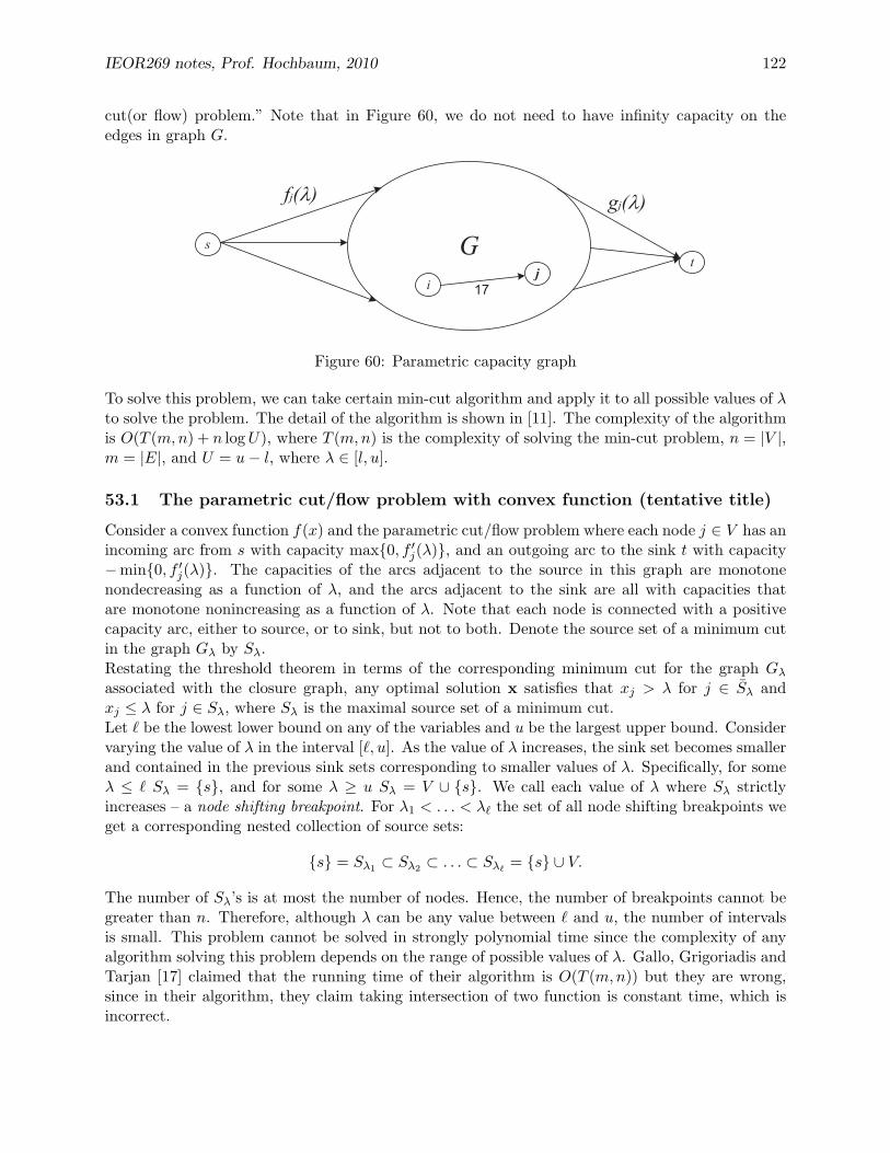
IEOR269 notes, Prof. Hochbaum, 2010 122
cut(or flow) problem.” Note that in Figure 60, we do not need to have infinity capacity on theedges in graph G.
Gs
t
ij
17
fj(l) gj(l)
Figure 60: Parametric capacity graph
To solve this problem, we can take certain min-cut algorithm and apply it to all possible values of λto solve the problem. The detail of the algorithm is shown in [11]. The complexity of the algorithmis O(T (m,n) + n logU), where T (m,n) is the complexity of solving the min-cut problem, n = |V |,m = |E|, and U = u− l, where λ ∈ [l, u].
53.1 The parametric cut/flow problem with convex function (tentative title)
Consider a convex function f(x) and the parametric cut/flow problem where each node j ∈ V has anincoming arc from s with capacity max0, f ′j(λ), and an outgoing arc to the sink t with capacity−min0, f ′j(λ). The capacities of the arcs adjacent to the source in this graph are monotonenondecreasing as a function of λ, and the arcs adjacent to the sink are all with capacities thatare monotone nonincreasing as a function of λ. Note that each node is connected with a positivecapacity arc, either to source, or to sink, but not to both. Denote the source set of a minimum cutin the graph Gλ by Sλ.Restating the threshold theorem in terms of the corresponding minimum cut for the graph Gλassociated with the closure graph, any optimal solution x satisfies that xj > λ for j ∈ Sλ andxj ≤ λ for j ∈ Sλ, where Sλ is the maximal source set of a minimum cut.Let ` be the lowest lower bound on any of the variables and u be the largest upper bound. Considervarying the value of λ in the interval [`, u]. As the value of λ increases, the sink set becomes smallerand contained in the previous sink sets corresponding to smaller values of λ. Specifically, for someλ ≤ ` Sλ = s, and for some λ ≥ u Sλ = V ∪ s. We call each value of λ where Sλ strictlyincreases – a node shifting breakpoint. For λ1 < . . . < λ` the set of all node shifting breakpoints weget a corresponding nested collection of source sets:
s = Sλ1 ⊂ Sλ2 ⊂ . . . ⊂ Sλ` = s ∪ V.
The number of Sλ’s is at most the number of nodes. Hence, the number of breakpoints cannot begreater than n. Therefore, although λ can be any value between ` and u, the number of intervalsis small. This problem cannot be solved in strongly polynomial time since the complexity of anyalgorithm solving this problem depends on the range of possible values of λ. Gallo, Grigoriadis andTarjan [17] claimed that the running time of their algorithm is O(T (m,n)) but they are wrong,since in their algorithm, they claim taking intersection of two function is constant time, which isincorrect.

IEOR269 notes, Prof. Hochbaum, 2010 123
Note that although a parametric cut/flow problem cannot be solved in strongly polynomial time,the output of this problem is compact. The output is just those breakpoint with the nodes addedinto the current subset, Sλ.
54 Average k-cut problem
Given a graph G = (V,E), a k-cut is finding a set of edges whose removal would partition the graphto k connected components, denoted as V1, V2, . . . , Vk. The cost of a k-cut is the summation of thecosts (or weight) of those edges. Let C(Vi, Vj) be the total cost of the edges connecting Vi and Vj .The objective function of the average k-cut problem is given below.
min∑k
i=1C(Vi, V − Vi)2|k|
Another problem which is similar to the average k-cut problem is the strength problem with thefollowing objective function.
min∑k
i=1C(Vi, V − Vi)2(|k| − 1)
If we linearize the above two problem, the problem is actually k-cut problem. For k-cut problemwith fixed k, it is polynomial time solvable. However, in general, a k-cut problem is NP-hard.However, the average k-cut problem is easy, since we have
min∑k
i=1C(Vi, V − Vi)2|k|
≥ |k|C(S∗, T ∗)2|k|
=C(S∗, T ∗)
2
where C(S∗, T ∗) is a minimum 2-cut of the graph G with the optimal source node and sink nodein graph G. Note that to find the optimal source node and sink node, we have to check all possiblepairs of (s, t) ∈ V and find the minimum s− t cut solution of each pair of (s, t) and then comparethe values to find the best pair. Hence, the min 2-cut is the solution of this problem, which is easyto solve.Hence, the average k-cut problem can be solved in polynomial time for general k, but the strengthproblem is NP-complete.
55 Image segmentation problem
A graph theoretical framework is suitable for representing image segmentation and grouping prob-lems. The image segmentation problem is presented on an undirected graph G = (V,E), where V isthe set of pixels and E are the pairs of adjacent pixels for which similarity information is available.Typically one considers a planar image with pixels arranged along a grid. The 4-neighbors set upis a commonly used adjacency rule with each pixel having 4 neighbors – two along the vertical axisand two along the horizontal axis. This set up forms a planar grid graph. The 8-neighbors arrange-ment is also used, but then the planar structure is no longer preserved, and complexity of variousalgorithms increases, sometimes significantly. Planarity is also not satisfied for 3-dimensional im-ages, and in general clustering problems there is no grid structure and thus the respective graphsare not planar.The edges in the graph representing the image carry similarity weights. The similarity is inverselyincreasing with the difference in attributes between the pixels. In terms of the graph, each edge[i, j] is assigned a similarity weight wij that increases as the two pixels i and j are perceived to

IEOR269 notes, Prof. Hochbaum, 2010 124
be more similar. Low values of wij are interpreted as dissimilarity. However, in some contextsone might want to generate dissimilarity weights independently. In that case each edge has twoweights, wij for similarity, and wij for dissimilarity.The goal of then “normalized cut variant” problem is to minimize the ratio of the similarity betweenthe set of objects and its complement and the similarity within the set of objects. That is, givena graph G = (V,E), we would like to find a subset S ⊂ V , such that C(S, S) is very small andC(S, S) is very large. Hence, the objective function is
min∅6=S⊂V
C(S, S)C(S, S)
(47)
Note that we also need to have |S| ≥ 2 and |E(S)| ≥ 1, otherwise, the objective is undefined.Shi and Malik addressed in their work on segmentation [19] an alternative criterion to replaceminimum cut procedures. This is because the minimum cut in a graph with edge similarity weightscreates a bipartition that tends to have one side very small in size. To correct for this unbalancedpartition they proposed several types of objective functions, one of which is the normalized cut,which is a bipartition of V , (S, S), minimizing:
minS⊂V
C(S, S)d(S)
+C(S, S)d(S)
. (48)
where di =∑
[i,j]∈E wij denote the sum of edge weights adjacent to node i. The weight of a subsetof nodes B ⊆ V is denoted by d(B) =
∑j∈B dj referred to as the volume of B. Note that with the
notation above d(B) = C(B, V ).In such an objective function, the one ratio with the smaller value of d() will dominate the objectivevalue - it will be always at least 1
2 of the objective value. Therefore, this type of objective functiondrives the segment S and its complement to be approximately of equal size. Indeed, like the balancedcut problem the problem was shown to be NP-hard, [19], by reduction from set partitioning.Back to the original objective function, that is, equation 47. This objective function is equivalentto minimizing one term in (48). To see this, note that:
C(S, S)C(S, S)
=C(S, S)
d(S)− C(S, S)
=1
d(S)C(S,S)
− 1.
Therefore, minimizing this ratio is equivalent to maximizing d(S)C(S,S)
which in turn is equivalent
to minimizing the reciprocal quantity C(S,S)d(S) , which is the first term in equation 48. The optimal
solution in the bipartition S will be the one set for which the value of the similarity within, C(S, S),is the greater between the set and its complement.
55.1 Solving the normalized cut variant problem
A formulation for the problem is provided first, minS⊂VC1(S,S)C2(S,S) . This is a slight generalization of
normalized cut variant problem in permitting different similarity weights for the numerator, wij ,and denominator, w′ij .We begin with an integer programming formulation of the problem. Let
xi =
1 if i ∈ S0 if i ∈ S.

IEOR269 notes, Prof. Hochbaum, 2010 125
We define two additional sets of binary variables: zij = 1 if exactly one of i or j is in S; yij = 1 ifboth i or j are in S. Thus,
zij =
1 if i ∈ S, j ∈ S, or i ∈ S, j ∈ S0 if i, j ∈ S or i, j ∈ S,
,
yij =
1 if i, j ∈ S0 otherwise.
With these variables the following is a valid formulation (NC) of the normalized cut variant problem:
(NC) min∑wijzij∑w′ijyij
(49)
subject to xi − xj ≤ zij for all [i, j] ∈ E (50)xj − xi ≤ zji for all [i, j] ∈ E (51)yij ≤ xi for all [i, j] ∈ E (52)yij ≤ xj (53)
1 ≤∑
[i,j]∈E
yij ≤ |E| − 1 (54)
xj binary j ∈ V (55)zij binary [i, j] ∈ E (56)yij binary i, j ∈ V. (57)
To verify the validity of the formulation notice that the objective function drives the values of zijto be as small as possible, and the values of yij to be as large as possible. Constraint (50) and(51) ensure zij cannot be 0 unless both endpoints i and j are in the same set. On the other hand,constraint (52) and (53) ensure that yij cannot be equal to 1 unless both endpoints i and j are inS.Constraint (54) ensures that at least one edge is in the segment S and at least one edge is in thecomplement - the background. Otherwise the ratio is undefined in the first case, and the optimalsolution is to choose the trivial solution S = V in the second.Excluding the sum constraint, the problem formulation (NC) is easily recognized as a monotoneinteger programming with up to three variables per inequality according to the definition providedin Hochbaum’s [9]. That is, a problem with constraints of the form ax − by ≤ c + z, where a andb are nonnegative and the variable z appears only in that constraint. Such linear optimizationproblems were shown there to be solvable as a minimum cut problem on a certain associated graph.We can then linearizing the objective function and solve the following λ-question which asks whetherminS⊂V
C1(S,S)C2(S,S) < λ. The λ-question for the normalized cut’ problem can be stated as the following
linear optimization question:
Is there a feasible subset V ′ ⊂ V such that∑
[i,j]∈E wijzij − λ∑
[i,j]∈E w′ijyij < 0?
We note that the λ-question is the following monotone optimization problem,

IEOR269 notes, Prof. Hochbaum, 2010 126
xi
xj
yij wij
- w’ijwji
Figure 61: The basic gadget in the graph representation.
(λ-NC) min∑
[i,j]∈E wijzij − λ∑
[i,j]∈E w′ijyij
subject to xi − xj ≤ zij for all [i, j] ∈ Exj − xi ≤ zji for all [i, j] ∈ Eyij ≤ xi for all [i, j] ∈ Eyij ≤ xjyi∗j∗ = 1 and yi′j′ = 0xj binary j ∈ Vzij binary [i, j] ∈ Eyij binary i, j ∈ V.
If the optimal value of this problem is negative then the answer to the λ-question is yes, otherwisethe answer is no. This problem (λ-NC) is an integer optimization problem on a totally unimodularconstraint matrix. That means that we can solve the linear programming relaxation of this problemand get a basic optimal solution that is integer. Instead we will use a much more efficient algorithmdescribed in [9] which relies on the monotone property of the constraints.
55.2 Solving the λ-question with a minimum cut procedure
We construct a directed graph G′ = (V ′, A′) with a set of nodes V ′ that has a node for each variablexi and a node for each variable yij . The nodes yij carry a negative weight of −λwij . The arc fromxi to xj has capacity w′ij and so does the arc from xj to xi as in our problem wij = wji. The twoarcs from each edge-node yij to the endpoint nodes xi and xj have infinite capacity. Figure 61shows the basic gadget in the graph G′ for each edge [i, j] ∈ E.We claim that any finite cut in this graph, that has yi∗j∗ on one side of the bipartition and yi′j′
on the other, corresponds to a feasible solution to the problem λ-NC. Let the cut (S, T ), whereT = V ′ \ S, be of finite capacity C(S, T ). We set the value of the variable xi or yij to be equal to1 if the corresponding node is in S, and 0 otherwise. Because the cut is finite, then yij = 1 impliesthat xi = 1 and xj = 1.Next we claim that for any finite cut the sum of the weights of the yij nodes in the source set andthe capacity of the cut is equal to the objective value of problem λ-NC. Notice that if xi = 1 andxj = 0 then the arc from the node xi to node xj is in the cut and therefore the value of zij is equalto 1.We next create a source node s and connect all yij nodes to the source with arcs of capacity λw′ij .The node yi∗j∗ is then shrunk with a source node s and therefore also its endpoints nodes are

IEOR269 notes, Prof. Hochbaum, 2010 127
effectively shrunk with s. The node yi′j′ and its endpoints nodes are analogously shrunk with thesink t. We denote this graph illustrated in Figure 62, G′st.
!"#$%&'&()&'
*
+
!"
#$%& !%
!'
!&
!(
)"%
)%&
)&'
)'(
#$&'
#$'(
!,-.'&()&'
Figure 62: The graph G′st with edge [1, 2] as source seed and edge [4, 5] as sink seed.
Theorem 55.1. A minimum s, t-cut in the graph G′st, (S, T ), corresponds to an optimal solutionto λ-NC by setting all the variables whose nodes belong to S to 1 and zero otherwise.
Proof: Note that whenever a node yij is in the sink set T the arc connecting it to the source isincluded in the cut. Let the set of x variable nodes be denoted by Vx and the set of y variablenodes, excluding yi∗j∗ , be denoted by Vy. Let (S, T ) be any finite cut in G′st with s ∈ S and t ∈ Tand capacity C(S, T ).
C(S, T ) =∑
yij∈T∩Vy
λw′ij +∑
i∈Vx∩S,j∈Vx∩Twij
=∑v∈Vy
λw′v −∑
yij∈S∩Vy
λw′ij +∑
xi∈Vx∩S,xj∈Vx∩Twij
= λW ′ + [∑
i∈Vx∩S,j∈Vx∩Twij −
∑yij∈S∩Vy
λw′ij ].
This proves that for a fixed constant W ′ =∑
v∈Vy w′v the capacity of a cut is equal to a constant
W ′λ plus the objective value corresponding to the feasible solution. Hence the partition (S, T )minimizing the capacity of the cut minimizes also the objective function of λ-NC. Lec13

IEOR269 notes, Prof. Hochbaum, 2010 128
56 Duality of Max-Flow and MCNF Problems
56.1 Duality of Max-Flow Problem: Minimum Cut
Given G = (V,E), capacities uij for all (i, j) ∈ E and two special nodes s, t ∈ V , consider theformulation of the maximum flow problem. Let xij be the variable denoting the flow on arc (i, j).
max xtssubject to
∑i xki −
∑j xjk = 0 ∀k ∈ V
0 ≤ xij ≤ uij ∀(i, j) ∈ E.
For dual variables, let zij be the nonnegative dual variables associated with the capacity upperbounds constraints, and λi be the variables associated with the flow balance constraints. Thedual of the above formulation is given as follows:
min∑
(i,j)∈E uijzijsubject to zij − λi + λj ≥ 0 ∀(i, j) ∈ E
λs − λt ≥ 1zij ≥ 0 ∀(i, j) ∈ E.
The dual problem has an infinite number of solutions: if (λ∗, z∗) is an optimal solution, then sois (λ∗ + δ, z∗) for any constant δ. To avoid that we set λt = 0 (or to any other arbitrary value).Observe now that with this assignment there is an optimal solution with λs = 1 and a partition ofthe nodes into two sets: S = i ∈ V |λi = 1 and S = i ∈ V |λi = 0.The complementary slackness condition states that the primal and dual optimal solutions x∗, λ∗, z∗
satisfy,x∗ij · [z∗ij − λ∗i + λ∗j ] = 0
[uij − x∗ij ] · z∗ij = 0.
In an optimal solution z∗ij − λ∗i + λ∗j = 0 so the first set of complementary slackness conditions donot provide any information on the primal variables xij. As for the second set, z∗ij = 0 on allarcs other than the arcs in the cut (S, S). So we can conclude that the cut arcs are saturated, butderive no further information on the flow on other arcs.The only method known to date for solving the minimum cut problem requires finding a maximumflow first, and then recovering the cut partition by finding the set of nodes reachable from thesource in the residual graph (or reachable from the sink in the reverse residual graph). That set isthe source set of the cut, and the recovery can be done in linear time in the number of arcs, O(m).On the other hand, if we are given a minimum cut, there is no efficient way of recovering the flowvalues on each arc other than essentially solving the max-flow problem from scratch. The onlyinformation given by the minimum cut, is the value of the maximum flow and the fact that the arcson the cut are saturated. Beyond that, the flows have to be calculated with the same complexityas would be required without the knowledge of the minimum cut.
56.2 Duality of MCNF problem
Consider the following formulation of the Minimum Cost Network Flow Problem. Given a networkG = (V,E) with a cost cij and an upper bound uij associated with each directed arc (i, j), Also,bi represent the supplies for every node in the network, where bi < 0 implies a demand node. The

IEOR269 notes, Prof. Hochbaum, 2010 129
problem can be formulated as an LP in the following way:
max∑n
j=1
∑ni=1 cijxij
subject to∑
k∈V xik −∑
k∈N xki = bi ∀i ∈ V0 ≤ xij ≤ uij ∀(i, j) ∈ E
Once again, let the dual variables be zij as the nonnegative dual variables associated with thecapacity upper bounds constraints, and λi as the free variables associated with the flow balanceconstraints.
Hence the dual formulation of MCNF would be as follows:
min∑
(i,j)∈E uijzij +∑
i∈V λibisubject to zij − λi + λj ≥ cij ∀(i, j) ∈ E
zij ≥ 0 ∀(i, j) ∈ E
With the addition of the costs cij for every edge i, j ∈ E, the resulting monotone inequality in thedual fomulation now includes an extra constant term, cij .Hence, the presence of a constant term in a monotone inequality in three variables (λi, λj andzij) is an indication of the formulation being a dual of a minimum cost network flow problem, asopposed to a maximum flow problem. This implies that the problem can no longer be solved asa minimum cut problem (as was the case with Max-Flow), but is still solvable in polynomial timebecause the constraint matrix is total unimodular (TUM).
57 Variant of Normalized Cut Problem
Consider a graph, G = (V,E), with a weight wij assicated with each edge.Let S be a subset of V and C(S, S) be the capacity of the cut between S and the rest of the graph(S). Also let C(S,S) be the sum of the weights of all the edges contained in the subgraph composedof S, and C(S,V) be the sum of edges with atleast one endpoint in S.The variant of the normalized cut problem (NC ′) is given as follows:
min∅6=S⊂VC(S,S)C(S,S) (NC ′)
Let qi be defined as the sum of weights of all adjacent edges to i ∈ V . Hence, based on the abovedefinitions, the following relationships exist:
qi =∑
j|(i,j)∈E wijC(S, V ) = C(S, S) + C(S, S)∑
i∈S qi =∑
i∈S∑
j|(i,j)∈E wij = C(S, S) + C(S, V )
The first equality reiterates the definition of qi, while the second equality shows that the sum ofthe weights of the edges with one node in S is equal to the sum of the edge weights with both nodesin S and exactly one node in S. Combining the first two relationships, we obtain the third equalitysince C(S,S) gets repeated twice ( for both i, j ∈ S).Based on the above-defined relationships, one can now observe the following equivalences:
min∅6=S⊂VC(S,S)∑i∈S qi
⇔ C(S,S)2C(S,S)+C(S,S)
⇔ 1
2C(S,S)
C(S,S)+1

IEOR269 notes, Prof. Hochbaum, 2010 130
Since,C(S,S)C(S,S) ∝ 1
2C(S,S)
C(S,S)+1
this leads to an alternate formulation for NC ′:
min∅6=S⊂VC(S,S)∑i∈S qi
In order to linearize the ratio form of NC ′, the λ− question can be asked as follows:
min∅6=S⊂V C(S, S)− λ∑
i∈S qi < 0
57.1 Problem Setup
Consider the following set of decision variables:
xi =
1 if i ∈ S0 otherwise
zij =
1 if i ∈ S, j ∈ S0 otherwise
Therefore, the variant of the normalized cut problem can be formulated as follows:
min∑
i,j∈E wijzij − λ∑
j∈V qjxjsubject to xi − xj ≤ zij ∀(i, j) ∈ E
0 ≤ xi ≤ 1 ∀i ∈ V0 ≤ zij ∀(i, j) ∈ E
Observe the following points about the formulation:
• Since the constraint matrix is totally unimodular, xj need not be restricted as an integer,while zij only needs to be constrained with a lower bound. Hence, the problem can be solvedas an LP.
• In general, the parameters of the node weights, qj and edge weights, wij need not be relatedto each other, i.e. ”qi =
∑j|(i,j)∈E wij” is not required for the problem to be solved. However,
while qj can be negative or positive, negative wij makes the problem NP-hard.
• In a closure problem, the closure constraint is of the following form:
xi ≤ xj ⇔ xi − xj ≤ 0
However, in our formulation, we relax the closure constraint. Hence, for any pair of of vertices(i, j) which violates the closure property, there is an associated penalty cost, wij , introducedthrough the means of the variable zij :
xi − xj ≤ zij
• The above-mentioned formulation, with a transformation of minimization to maximization,can be seen as an instance of the maximum s-excess problem (see section 57.3).
Before discussing the solution methodology for the variant of the normalized cut problem, let usreview the concepts of the maximum closure and the s-excess problems, in order to appreciate therelationship between them.
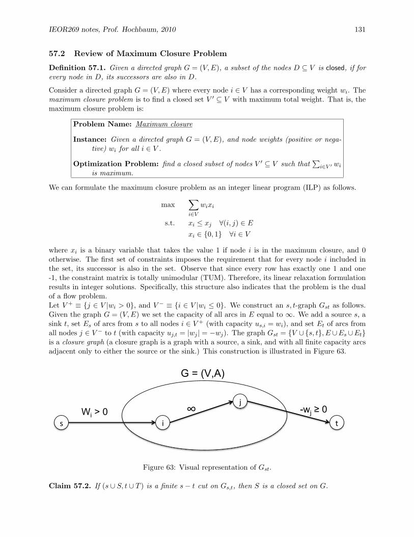
IEOR269 notes, Prof. Hochbaum, 2010 131
57.2 Review of Maximum Closure Problem
Definition 57.1. Given a directed graph G = (V,E), a subset of the nodes D ⊆ V is closed, if forevery node in D, its successors are also in D.
Consider a directed graph G = (V,E) where every node i ∈ V has a corresponding weight wi. Themaximum closure problem is to find a closed set V ′ ⊆ V with maximum total weight. That is, themaximum closure problem is:
Problem Name: Maximum closure
Instance: Given a directed graph G = (V,E), and node weights (positive or nega-tive) wi for all i ∈ V .
Optimization Problem: find a closed subset of nodes V ′ ⊆ V such that∑
i∈V ′ wiis maximum.
We can formulate the maximum closure problem as an integer linear program (ILP) as follows.
max∑i∈V
wixi
s.t. xi ≤ xj ∀(i, j) ∈ Exi ∈ 0, 1 ∀i ∈ V
where xi is a binary variable that takes the value 1 if node i is in the maximum closure, and 0otherwise. The first set of constraints imposes the requirement that for every node i included inthe set, its successor is also in the set. Observe that since every row has exactly one 1 and one-1, the constraint matrix is totally unimodular (TUM). Therefore, its linear relaxation formulationresults in integer solutions. Specifically, this structure also indicates that the problem is the dualof a flow problem.Let V + ≡ j ∈ V |wi > 0, and V − ≡ i ∈ V |wi ≤ 0. We construct an s, t-graph Gst as follows.Given the graph G = (V,E) we set the capacity of all arcs in E equal to ∞. We add a source s, asink t, set Es of arcs from s to all nodes i ∈ V + (with capacity us,i = wi), and set Et of arcs fromall nodes j ∈ V − to t (with capacity uj,t = |wj | = −wj). The graph Gst = V ∪s, t, E ∪Es ∪Etis a closure graph (a closure graph is a graph with a source, a sink, and with all finite capacity arcsadjacent only to either the source or the sink.) This construction is illustrated in Figure 63.
s i
j
t
G = (V,A)
-wj ≥ 0 Wi > 0 ∞
Figure 63: Visual representation of Gst.
Claim 57.2. If (s ∪ S, t ∪ T ) is a finite s− t cut on Gs,t, then S is a closed set on G.

IEOR269 notes, Prof. Hochbaum, 2010 132
Proof. Assume by contradiction that S is not closed. This means that there must be an arc(i, j) ∈ E such that i ∈ S and j ∈ T . This arc must be on the cut (S, T ), and by constructionui,j =∞, which is a contradiction on the cut being finite.
Theorem 57.3. If (s∪ S, t∪ T ) is an optimal solution to the minimum s− t cut problem on Gs,t,then S is a maximum closed set on G.
Proof.
C (s ∪ S, t ∪ T ) =∑
(s,i)∈Est, i∈T
us,i +∑
(j,t)∈Est, j∈S
uj,t
=∑
i∈T∩V +
wi +∑
j ∈S∩V −−wj
=∑i∈V +
wi −∑
i∈S∩V +
wi −∑
j∈S∩V −wj
= W+ −∑i∈S
wi
(Where W+ =∑
i∈V + wi, which is a constant.) This implies that minimizing C(s ∪ S, t ∪ T ) isequivalent to minimizing W+ −
∑i∈S wi, which is in turn equivalent to maxS⊆V
∑i∈S wi.
Therefore, any source set S that minimizes the cut capacity also maximizes the sum of the weightsof the nodes in S. Since by Claim 57.2 any source set of an s− t cut in Gs,t is closed, we concludethat S is a maximum closed set on G.
57.3 Review of Maximum s-Excess Problem
Problem Name: Maximum s-Excess
Instance: Given a directed graph G = (V,E), node weights (positive or negative)wi for all i ∈ V , and nonnegative arc weights cij for all (i, j) ∈ E.
Optimization Problem: Find a subset of nodes S ⊆ V such that∑i∈S wi −
∑i∈S,j∈S cij is maximum.
The s-excess problem is closely related to the maximum flow and minimum cut problems as shownnext.
Lemma 57.4. For S ⊆ V , s ∪ S is the source set of a minimum cut in Gst if and only if S is aset of maximum s-excess capacity C(s, S)− C(S, S ∪ t) in the graph G.
Proof: We rewrite the objective function in the maximum s-excess problem:
maxS⊆V [C(s, S)− C(S, S ∪ t)] = maxS⊆V [C(s, V )− C(s, S)− C(S, S ∪ t)]= C(s, V )−minS⊆V [C(s, S) + C(S, S ∪ t)].
In the last expression the term C(s, V ) is a constant from which the minimum cut value issubtracted. Thus the set S maximizing the s-excess is also the source set of a minimum cut and,vice versa – the source set of a minimum cut also maximizes the s-excess.

IEOR269 notes, Prof. Hochbaum, 2010 133
57.4 Relationship between s-excess and maximum closure problems
The s-excess problem is a natural extension of the maximum closure problem. The maximumclosure problem is to find in a node weighted graph a subset of nodes that forms a closed set, (i.e.with each node in a closed set all its successors are in the set as well), so that the total weight ofthe nodes in the closed subset is maximized. The s-excess problem may be viewed as a maximumclosure problem with a relaxation of the closure requirement: Nodes that are successors of othernodes in S (i.e. that have arcs originating from node of S to these nodes) may be excluded fromthe set, but at a penalty that is equal to the capacity of those arcs.With the discussion in the previous section we conclude that any maximum flow or minimum cutalgorithm solves the maximum s-excess problem: The source set of a minimum cut is a maximums-excess set.
57.5 Solution Approach for Variant of the Normalized Cut problem
Figure 64: s− t graph for the Variant of the Normalized Cut.
Given the graph G = (V,E), in order to construct a s− t graph, a source node has to be generatedby randomly selecting a node q ∈ V , since all the node weights are negative, i.e. -λqj < 0 ∀j ∈ V .Let V + ≡ q, and V − ≡ j ∀ V \q. We construct an s − t graph Gst as follows: we set thecapacity of all arcs in E equal to wij . We add a source s, a sink t, set Es of arcs from s to q (withcapacity us,q = 0), and set Et of arcs from all nodes j ∈ V − to t (with capacity uj,t = −λqj). Hencefigure 64 represents a generalization of the closure graph (figure 63), wherein the edge weights canhave finite costs, wij , as opposed to ∞ in (figure 63).
With the modified graph Gst, the variant of the normalized cut problem can be solved as follows:
1. Select a source node, q ∈ V and solve the parametric cut problem: the partition containsat least q in the source set.
2. Since q is chosen at random, iterate on different values of q to find different solutions tothe λ− question.
3. The optimal value would be the minimum amongst the different solutions.

IEOR269 notes, Prof. Hochbaum, 2010 134
The parametric cut problem is solved for all breakpoints of λ (which are bounded by the numberof nodes, n) with the same complexity as a single cut. Since the capacities are linear functionsof λ, the parametric cut problem, and hence the normalized cut problem, is strongly polynomialsolvable with the complexity of O(mincut(‖V ‖, ‖E‖)).Lec14)
58 Markov Random Fields
Markov Random Fields can be used for image reconstruction or segmentation. In image recon-struction, the objective is to assign a color to each pixel such that the assignment approximatesthe noisy observations, but is similar to neighboring pixels. The reconstructed image is a smoothedversion of the observed image.A graph G = (V,A) represents the image being considered. The vertices of the graph representpixels in the image. The arcs in the graph represent adjacency relations between pixels; if pixelsi and j are adjacent, then G will have directed arcs (i, j) and (j, i). Graph G allows image re-construction to be cast as an MRF problem (Eq. 58). Let each vertex i have an observed color giand an assigned color xi. Function Gi is the deviation cost, and penalizes the color assignment ofeach pixel according to its deviation from the observed value of the same pixel. Function Fij is theseparation cost, and penalizes the difference in color assignments between neighboring pixels.
min∑i∈V
Gi(gi, xi) +∑
(i,j)∈A
Fij (xi − xj) (58)
subject to xi ∈ [1, k] ∀i ∈ V
Let zij = xi−xj . When the separation cost Fij is monotone increasing, this equality (zij = xi−xj)constraint is equivalent to an inequality constraint (xi − xj ≤ zij). Eq. 58 can then be stated asthe image segmentation problem [10] of Eq. 59.
min∑i∈V
Gi(xi) +∑
(i,j)∈A
Fij (zij)
subject to li ≤ xi ≤ ui ∀i ∈ Vxi − xj ≤ zij ∀ (i, j) ∈ Azij ≥ 0 ∀ (i, j) ∈ A
1. Gi convex Fij linear : There is no known strongly polynomial algorithm for solving this case.One solution to this case consists of generating all n integer node shifting breakpoints usinga parametric cut, and then finding all the integer minima of the convex deviation costs foreach range between breakpoints [10].
Let T (m,n) denote the cost of solving minimum s,t cut on a graph with n nodes and m arcs;for example T (m,n) = O(mn log n2/m) if using the push-relabel algorithm.
Let U = max∀i,j∈V (ui − lj). The convex deviation costs can be a function of any value in U .Using a binary search over range U , n convex deviation costs must be evaluated at each stepof the search.

IEOR269 notes, Prof. Hochbaum, 2010 135
The time complexity is given by:
O (T (m,n) + n logU) (59)
2. Gi convex Fij convex : In this case, the objective is the sum of separable convex cost functions(deviation cost and separation cost). This problem can be solved as the convex cost integerdual network flow problem [13, 4, 5]. With the separation cost coefficients given by cij , thecomplexity is:
O (T (m,n) log(nC)) (60)C = max
(i,j)∈A(cij , k)
3. Gi nonlinear Fij convex : Consider a special case of MRF problem, where Fij =∞M zij , with
∞M being a very large number. In this special case, all zij variables will be optimally assignedzero, and the problem reduces to Eq. 61. With nonlinear Gi, even this special case is NP-hardsince it is necessary to evaluate Gi(xi) for all xi. In this special case, if Gi were convex, theproblem would be convex cost closure, and could be solved using minimum cut [22, 11].
min∑i∈V
Gi(xi) (61)
subject to xi ≤ xjli ≤ xi ≤ ui
4. Gi linear, Fij nonlinear: With nonlinear separation costs, the problem is NP-hard, as isstated in [10]. One particular discontinuous separation function that leads to NP-hardness isgiven in [2].
59 Examples of 2 vs. 3 in Combinatorial Optimization
Many problems in combinatorial optimization change from polynomial complexity to being NP-hard when some aspect of the input goes from size 2 to size 3. The following subsections presentproblem instances where this occurs.
59.1 Edge Packing vs. Vertex Packing
Edge packing is the same as the maximum matching problem. Given a graph G = (V,E), the goal ofedge packing is to find a maximum subset of edges S ⊆ E such that each node is incident to no morethan one. Edge packing is given by Eq. 62. Note that each xij appears in exactly two constraints, sothe constraint matrix is totally unimodular. Edge packing is polynomial time solvable; for example,Micali and Vazirani present an algorithm for solving edge packing in O(
√V E) [20].
xij =
1 (ij) ∈ S0 otherwise
.

IEOR269 notes, Prof. Hochbaum, 2010 136
max∑
(i,j)∈E
xij (62)
subject to∑ij∈E
xij ≤ 1 ∀j ∈ V
xij ∈ 0, 1
Vertex packing is another name for independent set. Given a graph G = (V,E), the goal of vertexpacking is to choose a maximum subset S ⊆ V of vertices such that no two share an edge. Moreformally, vertex packing is given by Eq. 63. Vertex packing is NP-hard if the degree of G is 3 orgreater, and has polynomial complexity on graphs of degree 2.
xi =
1 ifi ∈ S0 otherwise
.
max∑i∈V
xi (63)
subject to xi + xj ≤ 1 ∀(i, j) ∈ Exi ∈ 0, 1
59.2 Chinese Postman Problem vs. Traveling Salesman Problem
The Chinese Postman Problem (CPP) is given by Eq. 64. Both the undirected and directed casesof CPP can be solved in polynomial time.
xij =
1 (i, j) ∈ optimaltour0 otherwise
.
min∑i,j∈A
cijxij (64)
subject to xij ≥ 1 ∀(i, j) ∈ A∑(i,j)∈Ai∈V
xij −∑
(j,k)∈Ak∈V
xjk = 0 ∀j ∈ V
xi ∈ 0, 1
CPP on an undirected graph G can be solved via formulation as a matching problem. Note thatat each vertex of odd degree, some edges must be traversed multiple times. Create fully connectedgraph GODD = (V,E), where V is the set of all odd-degree vertices in G. The edge weights onE are all pairs shortest paths. Note that all-pairs shortest path is found in O(n3) using dynamicprogramming [6, 25]. Find a minimum matching on GODD; the corresponding edges from originalgraph G are the edges to be traversed twice. An Eulerian tour of G completes the solution to theundirected CPP problem.

IEOR269 notes, Prof. Hochbaum, 2010 137
CPP on a directed graph can be solved via formulation as a transportation problem. Createda subgraph G = (V,A) consisting of all vertices from G for which the indegree and outdegreediffer. The demand of each vertex in G is equal to its outdegree − indegree. The arcs are theshortest paths from each negative demand node to each positive demand node. The solution to thetransportation problem is then the set of arcs that must be traversed twice in the optimal CPPtour. The remainder of the solution is an Eulerian path in G.Traveling Salesman Problem (TSP) is NP-hard. To create directed graph G = (V,A), replace eachundirected edge (i, j) with 2 directed arcs (i, j) and (j, i). The solution to TSP is a minimum costvertex tour of G, with constraints on indegree and outdegree of each vertex, and constraints forsubtour elimination (Eq. 65). The NP-hard problem of finding a Hamiltonian circuit [7] reduces toTSP.
xij =
1 (i, j) ∈ optimaltour0 otherwise
.
min∑i,j∈A
cijxij (65)
subject to∑
(i,j)∈Ai∈V
xij = 1 ∀j ∈ V
∑(i,j)∈Aj∈V
xij = 1 ∀i ∈ V
∑i∈S
j∈V/S
xij ≥ 1 ∀S ⊂ V
xi ∈ 0, 1
59.3 2SAT vs. 3SAT
A 2SAT clause is of the form xi ∨ xj . In a satisfying assignment, at least one of the two literalsin the clause must be true, so the implications ¬xi =⇒ xj and ¬xj =⇒ xi must hold. Animplication graph G = (V,A) can thus be constructed, with an arc leading from each literal to itsimplication. A 2SAT problem is satisfiable if and only if no literal implies its negation. Stateddifferently, a 2SAT problem is satisfiable if and only if no variable appears as both a positive andnegative literal in the same strongly connected component15 of the graph [18]. Strongly connectedcomponents can be found in linear time using Tarjan’s algorithm [24]. Therefore, 2SAT can besolved in O(m), where m is the number of clauses [18].3SAT is well known to be NP-Hard [3], and this can be shown by reducing satisfiability16 to3SAT [15]. Unlike 2SAT, a 3SAT problem cannot be translated into an implication graph, since anunsatisfied literal only implies that one or more of the two other literals in the clause are satisfied.
59.4 Even Multivertex Cover vs. Vertex Cover
An even multivertex cover of a graph G = (V,E) is a minimum cost assignment of integers tovertices such that the assignments to the two vertices incident on each edge sum to an even number
15A strongly connected component is a subgraph in which there is a path from each vertex to every other vertex16with unrestricted clause size
IEOR269 notes, Prof. Hochbaum, 2010 138
(Eq. 66). Let xi represent the assignment to vertex i. Recall that the LP relaxation of vertex coveryields a half-integral solution. The following steps outline how the half-integral solution to vertexcover yields a integral solution to even multivertex cover. Since the LP relaxation can be solved inpolynomial time, then even multivertex cover can be solved in polynomial time.
1. Convert an even multivertex cover to vertex cover by changing the 2 to 1 on the right handside of the first constraint.
2. Solve the LP relaxation of vertex cover, yielding a half-integral solution.
3. Multiply the solution by 2, thus changing it from half-integral to integral. Each edge thatwas covered once is now covered twice.
min∑i∈V
wixi (66)
subject to xi + xj ≥ 2 ∀(i, j) ∈ Exi ≥ 0 ∀i ∈ Vxi ∈ Z
The NP-hard vertex cover problem on graph G = (V,E) is to find a minimum cost subset of verticesS ⊆ V that cover each edge (Eq. 67). While the LP relaxation can be solved in polynomial timeto produce a half-integral solution, there is no known polynomial time algorithm for optimallyrounding it to an integer solution. This is why vertex cover is more difficult than edge cover. Toshow that vertex cover is NP-hard for cubic and higher degree graphs, Karp uses a reduction fromclique [15].
xi =
1 vi ∈ S0 otherwise
.
min∑i∈V
wixi (67)
subject to xi + xj ≥ 1 ∀(i, j) ∈ Exi ∈ 0, 1
59.5 Edge Cover vs. Vertex Cover
Edge cover is polynomial time solvable. Given a graph G = (V,E), a minimum edge cover is aminimum subset S ⊆ E, such that all vertices in the graph are incident on one or more edges in S.Unweighted minimum edge cover is then given by Eq. 68.
xij =
1 (i, j) ∈ S0 otherwise
.
min∑
(i,j)∈E
xij (68)
subject to∑
(i,j)∈E
xij ≥ 1 ∀i ∈ V
xij ∈ 0, 1

IEOR269 notes, Prof. Hochbaum, 2010 139
Edge cover can be solved in polynomial time by first finding a maximum matching (Eq. 69). Letsubset M ⊂ E be a maximum matching of G. If M happens to be a perfect matching, then it isalso a minimum edge cover. Otherwise, M contains the maximum possible number of edges suchthat each one covers two unique vertices. The minimum edge cover can be created by adding toM , one additional edge to cover each vertex not covered by M . Since maximum matching can besolved in O(
√V E) [20], edge cover can also be solved with this same complexity. Weighted edge
cover is also polynomial time solvable, but extra steps are required; this was not covered in lecture.
xij =
1 (i, j) ∈M0 otherwise
.
max∑
(i,j)∈E
xij (69)
subject to∑
(i,j)∈E
xij ≤ 1 ∀i ∈ V
xij ∈ 0, 1
Recall from Sec. 59.4 that vertex cover is NP-hard for cubic and higher degree graphs. As previouslymentioned, this can be shown using reduction from clique [15].
59.6 IP Feasibility: 2 vs. 3 Variables per Inequality
IP feasibility with 2 variables per inequality can be solved in pseudo-polynomial time by binarizing.Initially, each constraint is of the form:
aijxi + akjxk ≤ bkEach integer variable xi is replaced by U binary variables xil(l = 1, . . . U). Let xil have the followingmeaning: xij is 1 if and only if xi ≥ l. Naturally, the constraint of Eq. 70 exists.
xil ≤ xi,l+1 ∀l ∈ 0, 1, . . . U − 1 (70)
Let αkl be defined as follows:
αkl = bbk − laijbij
c − 1 ∀l ∈ 0, 1 . . . U
An assignment is feasible if and only if one of the following inequalities hold for each value ofl(l = 1, . . . U):
xi ≤ l − 1 or xj ≤ αkl + 1
Using the binary representation of xi, the above inequalities are equivalent to:
xil = 0 or xj,αkl = 0
The above disjunction can be rewritten as:
xil + xj,αkl ≤ 1 (71)

IEOR269 notes, Prof. Hochbaum, 2010 140
In total, the problem now contains only 2 binary variables per constraint (Eq. 70 and Eq. 71), andall coefficients are either 1 or -1. Finding an IP feasible solution is equivalent to solving 2SAT, sinceeach constraint from Eq. 70 and Eq. 71 is equivalent to a SAT clause with two binary variables.Thus, IP feasibility problem reduces to 2SAT in polynomial time. As discussed in Sec. 59.3, 2SATcan be solved in time that is linear to the number of clauses. However, since the number of 2SATclauses is a function of U , the problem is only solvable in pseudo-polynomial time O(mU).With three variables per inequality, the IP feasibility problem cannot be reduced to 2SAT. Thisproblem is a general IP and is NP-hard.
References
[1] D. Greig B. Porteous, A. Seheult. Exact maximum a posteriori estimation for binary images.Journal of the Royal Statistical Society, Series B, 51(2):271–279, 1989.
[2] Y. Boykov, O. Veksler, and R. Zabih. A new algorithm for energy minimization with disconti-nuities. In Energy Minimization Methods in Computer Vision and Pattern Recognition, pages730–730. Springer, 1999.
[3] S. A. Cook. The complexity of theorem-proving procedures. In Proceedings of the third annualACM symposium on Theory of computing, page 158. ACM, 1971.
[4] R. K. Ahuja D. S. Hochbaum, J. B. Orlin. Solving the convex cost integer dual network flowproblem. Management Science, 49(7):950–964, 2003.
[5] R. K. Ahuja D. S. Hochbaum, J. B. Orlin. A cut based algorithm for the convex dual of theminimum cost network flow problem. Algorithmica, 39(3):189–208, 2004.
[6] R.W. Floyd. Algorithm 97: shortest path. Communications of the ACM, 5(6):345, 1962.
[7] M. R. Garey and D. S. Johnson. Computers and intractability. Freeman San Francisco, 1979.
[8] D. S. Hochbaum. An efficient algorithm for image segmentation, markov random fields andrelated problems. Journal of the ACM (JACM), 48(4):686–701, 2001.
[9] D. S. Hochbaum. Solving integer programs over monotone inequalities in three variables: Aframework for half integrality and good approximations. European Journal of OperationalResearch, 140(2):291–321, 2002.
[10] D. S. Hochbaum. The pseudoflow algorithm: A new algorithm for the maximum flow problem.Operations Research, 58(4):992–1009, July-Aug 2008.
[11] D. S. Hochbaum. Polynomial time algorithms for ratio regions and a variant of normalizedcut. IEEE Transactions on Pattern Analysis and Machine Intelligence, 32(5):889–898, 2010.
[12] D. S. Hochbaum and M. Queyranne. Minimizing a convex cost closure set. SIAM Journal ofDiscrete Math, 16(2):192–207, 2003.
[13] D. S. Hochbaum and J. G. Shanthikumar. Convex separable optimization is not much harderthan linear optimization. Journal of the ACM (JACM), 37(4):843–862, 1990.
[14] T. B. Johnson. Optimum Open Pit Mine Production Technology. PhD thesis, OperationsResearch Center, University of California, Berkeley, 1968.
IEOR269 notes, Prof. Hochbaum, 2010 141
[15] R. M. Karp. Reducibility among combinatorial problems. 50 Years of Integer Programming1958-2008, pages 219–241, 1972.
[16] Joseph B. Kruskal. On the shortest spanning subtree of a graph and the traveling salesmanproblem. Proceedings of the American Mathematical Society, 7(1):48–50, February 1956.
[17] G. Gallo M. D. Grigoriadis, R. E. Tarjan. A fast parametric maximum flow algorithm andapplications. SIAM Journal on Computing, 18(30), 1989.
[18] B. Aspvall M. Plass, R. Tarjan. A linear-time algorithm for testing the truth of certainquantified boolean formulas. Information Processing Letters, 8:121–123, 1979.
[19] J. Malik and J. Shi. Normalized cuts and image segmentation. IEEE Trans. Pattern Anal.Mach. Intell., 22(8):888–905, 2000.
[20] S. Micali and V.V. Vazirani. An O (4 |V| |E|) algorithm for finding maximum matching ingeneral graphs. In Foundations of Computer Science, 1980., 21st Annual Symposium on, pages17–27, 1980.
[21] Christos H. Papadimitriou and Kenneth Steiglitz. Combinatorial Optimization: Algorithmsand Complexity. Prentice-Hall.
[22] J. C. Picard. Maximal closure of a graph and applications to combinatorial problems. Man-agement Science, 22:1268–1272, 1976.
[23] R. C. Prim. Shortest connection networks and some generalizations. Bell Systems TechnicalJournal, pages 1389–1401, November 1957.
[24] R. Tarjan. Depth-first search and linear graph algorithms. In Switching and Automata Theory,1971., 12th Annual Symposium on, pages 114–121, 1971.
[25] S. Warshall. A theorem on boolean matrices. Journal of the ACM (JACM), 9(1):11–12, 1962.