iii debt: states’ medium-term fiscal challenge

27

Debt: States’ Medium-Term Fiscal ChallengeIII

1. Introduction

3.1 Summarising the analysis of states’

budgetary outcomes during 2017-20, as set

out in the foregoing Chapter, it is observed

that shortfalls in revenue receipts vis-à-

vis budgeted targets triggered larger than

expected compression in expenditure. While

this anchored fiscal prudence as reflected

in the conventional indicator, i.e., the GFD-

GDP ratio, there have been unintended

consequences as well which may have

implications for debt sustainability in the

medium-term.

3.2 First, there has been a reduction in the

overall size of the state budget in 2017-19.

This retarding fiscal impulse — accounting

for 44 per cent of the general government

deficit — has coincided with a cyclical

downswing in domestic economic activity

and may have inadvertently deepened

it. The slowdown in the economy can

debilitate revenue raising capacity and force

an increase in borrowing/future liabilities,

given downward rigidities confronted by

states under various expenditure heads, still

underwhelming revenue performance of the

Goods and Services Tax (GST) regime and

the shrinking financial autonomy that states’

face. Second, the narrowing balance sheet of

states is paradoxically associated with a rise

in debt and guarantees of State Public Sector

Enterprises (SPSEs). The risk of crystallisation

of these contingent charges on states’

finances has direct adverse implications for

debt sustainability in the medium-term.

3.3 It is in this context that debt

sustainability selects itself as the theme of

this year’s report, as outlined in Chapter 1.

The organising principle driving the rest of this

chapter is as follows. States’ indebtedness

in the future (Dt+1) is a linear combination of

the current stock of debt (Dt) and additions

to this stock, both budgetary (∆Bt) and extra/

off-budgetary (∆Ot), i.e.,

D t+1 = Dt + ∆Bt + ∆Ot …………………(1)

The slowdown in the economy poses a challenging fiscal environment for states as lower revenue raising capacity and downward rigidities in various expenditure heads can force an increase in borrowing/future liabilities. The weak performance of State Public Sector Enterprises (SPSEs), particularly in power distribution, continues to be a source of fiscal risk going forward if the off-budget liabilities get crystallised. Further, the increased orientation of state government borrowings towards markets brings attendant challenges of pricing, liquidity, management of redemption cycle and diversification of investor base. The debt position of state governments has started showing incipient signs of unsustainability, particularly post UDAY. Recognising that debt sustainability is closely linked to revenue generation of states, they will have to improve their revenue raising capacity by capitalising on the efficiency gains under the GST and digitisation and improving compliance. Also, turnaround of power distribution sector is crucial to avoid fiscal surprises going forward.

State Finances : A Study of Budgets of 2019-20

28

3.4 Accordingly, the rest of the Chapter is organised into Sections 2 to 7. Recognising that the revenue generation holds the key to prudent debt management and can act as a circuit breaker to debt spirals, Section 2 drills into fundamental drivers and brakes in various sources of revenue – own taxes; states’ share in GST; and non-tax revenue - and the scope for and the nature of tax reforms that may be desirable and feasible. With states entrusted with higher responsibilities relative to their revenue generation capacity, transfer of resources from the Centre to the states in the form of tax devolution and grants remains important and its share has also seen a rise in overall receipts in recent years. Accordingly, trends in Central fiscal transfers have been analysed in this section recognising that they supplement own revenue and augment debt servicing capacity.

3.5 State budgets have to also adjust to exogenous fiscal shocks, with attendant implications for indebtedness. In particular, the structural weakness in state-owned power distribution utilities has necessitated three instances of financial restructuring over the thirteen-year period – One Time Settlement (2003); Financial Restructuring Plan (2012); and Ujwal DISCOM Assurance Yojana (UDAY) (2015). These interventions have a cascading effect on debt and off-budget liabilities. With UDAY reaching its terminal year (2019-20), Section 3 assesses the different facets of the UDAY scheme in terms of its impact on state finances and future liabilities.

3.6 While the focus so far was on exploring into ∆B

t in equation (1), Section 4 undertakes an analysis of state government guarantees

to assess the balance of risks around the ∆Ot term of equation (1). In recent years, the financing mix of states’ fiscal deficit has evolved in favour of market borrowings, which pose attendant fiscal challenges for debt management in terms of liquidity and roll-over risks, redemption pressures and pricing. These issues are dealt with in Section 5. All this leads into an evaluation of the debt profile of states, from the perspective of different scenarios for ∆Bt and ∆Ot in Section 6. Concluding observations are set out in Section 7.

2. States’ Revenue

3.7 States’ revenue comprises of (i) own tax revenue and non-tax revenue; and (ii) transfers received from the Centre in the form of devolution of Central taxes and grants (Chart III.1).

3.8 From the late 1990s, states’ total revenue has been increasing as a proportion to GDP, albeit with variations over time and space. Since 2010-11, states’ revenue has recovered from the slowdown in domestic economic activity imposed by the global financial crisis. From 2014-15, increased transfers as recommended by FC-XIV and more recently, GST compensation cess have provided tailwinds (Chart III.2).

3.9 There is a marked difference across states in revenue collections. For instance, average own tax revenue is highest for Andhra Pradesh for 2011-18 period. In the North-Eastern states, narrower tax bases operate as constraints and accordingly they receive the highest transfers from the Centre (Chart III.3).

Debt: States’ Medium-Term Fiscal Challenge

29

2.1 Own Tax Revenue

3.10 Own taxes constitute 45 per cent of the total revenue (Chart III.1) of states. They mainly comprise taxes on commodities and

services (sales tax/Value Added Tax (VAT)/

GST) and stamp duties. Sales tax/VAT, now

replaced by the GST, constitutes almost

half of the total own tax revenue of states.


30

On average, own tax revenues have grown at

a rate of 14.7 per cent over the last decade

(Table III.1).

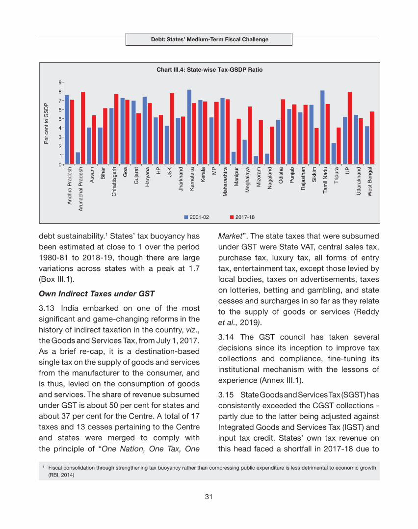
3.11 States with high tax-GSDP ratios at

the beginning of the century have witnessed

a moderation in the ratio while those with

lower initial tax-GSDP ratios have

improved between 2001-02 to 2017-18

(Chart III.4).

3.12 Enhancing tax buoyancy in states is

crucial for meeting expenditure commitments

and addressing the medium-term objective of

Table III.1: States’ Own Tax Revenue - Composition(Per cent)

Share in OTR Growth Per cent of GDP

1990s 2000s 2010-20 1990s 2000s 2010-20 1990s 2000s 2010-20

I. Own tax Revenue (II+III) 100.0 100.0 100.0 14.8 13.5 14.7 5.3 5.8 6.3

II. Direct Taxes

1. Taxes on income and expenditure 1.5 1.4 0.7 15.4 9.9 5.3 0.1 0.1 0.0

2. Taxes on property and capital transaction 9.9 12.0 12.1 15.0 16.9 13.9 0.5 0.7 0.8

Of which:

Stamp duties and registration fees 8.2 10.6 10.7 17.1 16.9 14.0 0.4 0.6 0.7

III. Indirect Taxes

3. Taxes on commodities and services 88.5 86.6 87.3 14.8 13.2 14.9 4.7 5.0 5.5

Of which:

Sales tax/VAT 59.3 60.9 52.0 15.4 13.6 5.9 3.1 3.5 3.5

Excise duties 14.5 12.6 12.0 14.8 12.5 14.0 0.8 0.7 0.8

Taxes on vehicles 5.6 5.6 5.4 16.0 12.1 15.3 0.3 0.3 0.3

Source: Budget documents of state governments.


31

debt sustainability.1 States’ tax buoyancy has been estimated at close to 1 over the period 1980-81 to 2018-19, though there are large variations across states with a peak at 1.7 (Box III.1).

Own Indirect Taxes under GST

3.13 India embarked on one of the most significant and game-changing reforms in the history of indirect taxation in the country, viz., the Goods and Services Tax, from July 1, 2017. As a brief re-cap, it is a destination-based single tax on the supply of goods and services from the manufacturer to the consumer, and is thus, levied on the consumption of goods and services. The share of revenue subsumed under GST is about 50 per cent for states and about 37 per cent for the Centre. A total of 17 taxes and 13 cesses pertaining to the Centre and states were merged to comply with the principle of “One Nation, One Tax, One

Market”. The state taxes that were subsumed under GST were State VAT, central sales tax, purchase tax, luxury tax, all forms of entry tax, entertainment tax, except those levied by local bodies, taxes on advertisements, taxes on lotteries, betting and gambling, and state cesses and surcharges in so far as they relate to the supply of goods or services (Reddy et al., 2019).

3.14 The GST council has taken several decisions since its inception to improve tax collections and compliance, fine-tuning its institutional mechanism with the lessons of experience (Annex III.1).

3.15 State Goods and Services Tax (SGST) has consistently exceeded the CGST collections - partly due to the latter being adjusted against Integrated Goods and Services Tax (IGST) and input tax credit. States’ own tax revenue on this head faced a shortfall in 2017-18 due to

1 Fiscal consolidation through strengthening tax buoyancy rather than compressing public expenditure is less detrimental to economic growth (RBI, 2014)


32

Box III.1: Tax Buoyancy at the State Level

States are largely dependent on tax devolution from the

Centre and their own tax revenue. In both cases, tax

buoyancy2 - the responsiveness of tax revenue to nominal

GDP changes – is key. For instance, the growth of own

tax revenue has not always been higher than nominal GDP

growth (Chart 1).

In this context, an operational distinction is often made

between short-run tax buoyancy, which helps to explain

the role of government in stabilising the economy over the

business/growth cycle, and long-run tax buoyancy, which

is the capacity of states to ensure fiscal sustainability in

the long-run (Belinga et al., 2014; Dudine and Jalles, 2017).

Tax buoyancy has been estimated at 1.30 for the period

2005-06 to 2010-11(Rajaraman et al., 2006), as against

the Twelfth Finance Commission’s estimate of 1.20. An

update of these estimates for the period 1980-81 to 2019-

20 establishes the existence of long-run cointegration3

between states’ taxes and their bases; given the long-

run coefficients, estimation of short-run coefficients is

attempted through error-correction models.4 Variables are

found to be integrated of order one. The coefficients of

log transformed variables provide direct estimates of tax

buoyancy (Table 1).

Short-run tax buoyancy of states’ own tax revenue is

estimated at 0.76, reflecting a weak automatic stabiliser.

Within own tax revenues, taxes on property and capital

transactions, and the SGST have short-run buoyancies

higher than unity, implying that they are effective automatic

stabilisers. Sales taxes and excise duties have low short-

run tax buoyancies, given the inelastic and nature of its

major components like petrol and alcohol.

Long-run buoyancy is estimated at 1.06, implying that

higher economic growth helps in containing fiscal deficits

and reduces debt through higher tax revenue. Long-run

tax buoyancy for all states’ taxes is greater than one.

Within these aggregate estimates are the large inter-state

variations, ranging from a low of 0.72 to a high of 1.66.

These estimates reflect successful efforts by some states

to improve buoyancy and the need for others to catch up

through reforms in tax architecture, widening the scope

and tax base, and rationalising rates under the GST and

efficiency in tax collection.

2 Buoyancy reflects the effect of both automatic stabilisers and discretionary policy changes; tax elasticity refers to the income effects of discretionary policy changes only.

3 Cointegration method establishes long-run relationship between variables, if they are integrated of order 1.4 If variables are cointegrated, error correction model estimates the short run coefficients and deviation from the long run path and how much

time does the system takes to revert to the equilibrium path.

(Contd.)


33

Table 1: Tax Buoyancy

Item

Share in Total

Own Tax Revenue (2019-20)

Tax buoyancy

Period: 1980-81 to 2018-19

Long Run Short Run

Own Tax Revenue 100.0 1.063*** 0.764**

Of Which:

Taxes on Property & Capital Transactions

11.3 1.179*** 1.371**

Taxes on Commodities and Services

88.2 1.054*** 0.678**

Of Which:

Sales Tax 23.2 1.052*** Not significant

State Excise 12.5 1.005*** 0.628**

SGST 43.5 - 1.670**

*** and ** refers to statistical significance at 1 and 5 per cent level. GDP used as base.Notes: 1. SGST includes IGST. 2. Tax Buoyancy of SGST is estimated using panel regression

for period 2017-18 to 2019-20.Source: RBI Staff Estimates.

References

Belinga V., D. Benedek, R. A. de Mooij and J. Norregaard

(2014), “Tax Buoyancy in OECD Countries”, IMF Working

Paper 110.

Dudine, Paolo and Joao Tovar Jalles (2017), “How Buoyant

is Tax system? New Evidence from a Large Heterogeneous

Panel”, IMF Working Paper, January.

Rajaraman, Indira, Rajan Goyal and Jeevan Kumar

Khudrakpam (2006), “Tax Buoyancy Estimates for India

States” , EPW, Vol. 41, Issue 16.

initial teething challenges associated with rate

revisions and sharing pattern of IGST among

states but they seem to have gained traction

in 2018-19. On a monthly basis also, states’

GST revenue seems to be stabilising after

witnessing some initial volatility and is broadly

on an uptrend (Chart III.5).

3.16 A cross-country event-study reveals

that the GST tax to GDP ratio gained

most traction in the year following the

implementation (t+1) but the revenues

settled downwards after two years albeit

higher than pre-GST levels for most countries

(Chart III.6).


34

3.17 In the case of India, GST collections have varied across states. Though the rationalisation of rates by the GST Council has brought down the effective weighted average GST rate from 14.4 per cent at the time of inception to 11.6 per cent; enhanced buoyancy has been achieved by widening the tax base and removing distortions (Chart III.7).

3.18 Barring a few states, however, the desired GST targets have proved elusive so far warranting compensation cess in the first two years of implementation. State-wise analysis shows that though the compensation cess increased in absolute amount in 2018-19 RE vis-à-vis 2017-18; as per cent of taxes on commodities and services, it declined for most of the states (with quite a few states lying below the 45 degree line in Chart III.8) and few states not requiring any compensation in 2018-19. This cushion, whereby states’ revenue shortfall under GST remains protected for first five years, should be effectively utilised as the compensation cess is slated to be eliminated

by 2021-22 as per GST (Compensation

to States) Act. Concerted efforts towards

raising GST revenue by plugging loopholes

and mitigating IT glitches are important.

Other steps could include putting in place

an invoice-matching system to facilitate

system validated input tax credit; fixing the


35

operational deficiencies in the payment module; alignment of system validations with the GST Acts and Rules; and alleviating system design deficiencies (CAG, 2019). The challenge for the GST Council is to

realise the full potential of GST for enhancing

tax-GDP ratio and work on other areas of

our economy to enhance its competitiveness

(Das, 2019).

3.19 Restructuring of the old administrative

set-up under VAT is the key to successful

tapping of the full potential under GST.

Accordingly, states may have to improve data

analytics, particularly by using the GSTN

network. Some states have started operating

and exploiting their own databases under the

GST regime to enhance revenue.

3.20 Currently, alcohol and petroleum

are still out of the purview of GST. For a

majority of the states, however, the sales tax

on petroleum forms about 15-20 per cent

of own tax revenue, while excise duty on

alcohol accounts for around 10-15 per cent5

(Chart III.9). Furthermore, the effective rates

5 This does not take into account fees for stamping, weights and measures applicable to liquor and VAT on alcohol, accordingly the actual collections might be higher than those reported here.


36

of taxes levied by states on petrol vary from

state to state – from 16 per cent in Goa to

39 per cent in Maharashtra for petrol, and

from 11 per cent in Mizoram to 28 per cent

in Andhra Pradesh for diesel. On average,

the effective tax rate levied by states is 28

per cent for petrol and 20 per cent for diesel.

The challenge is to subsume these two

major sources of revenue under GST while

maintaining revenue neutrality, keeping in view

its relevance to maintaining and rationalising

states’ debt.

Own Direct Taxes

3.21 Direct taxes applied by states include

taxes on income and taxes on property as

well as capital tax (mainly stamp duty and

registration fees). They constitute 11.7 per

cent of own tax revenue, with stamp duties

being the major component (10.5 per cent).

Over the years, the share of taxes on income

and expenditure has declined to low levels.

Under this head is also included the agricultural

income tax which currently is exempted from

income tax, irrespective of the size of income,

except those on plantations levied by states like Assam.6 While the share of taxes on income is declining, collections in respect of taxes on profession, trade and employment are rising but with large inter-state variations.7 The scope under tax base expansion for taxes on income and expenditure remains limited, thus, having minimal implications from the perspective of revenue mobilisation.

3.22 As regards stamp duties and registration fees, the reliance of state governments on revenue from these sources remains significant (more than 80 per cent of direct taxes and more than 10 per cent of own taxes), albeit with variation across states

(Table III.2). Revenue from this source is a

6 Not taxing agricultural income may encourage laundering of non-agricultural income as agricultural incomes for tax evasion (Kelkar, 2002; Niti Aayog 2017).

7 Many states are not levying this tax at all, and therefore, the contribution from tax on income and expenditure is almost negligible.

Table III.2: Stamp Duty Collections

As per cent of Direct Taxes

As per cent of Own Tax Revenue

States 2000-01 to

2009-10

2010-11 to

2018-19

2000-01 to

2009-10

2010-11 to

2018-19

Andhra Pradesh 78.3 86.5 8.7 8.2Arunachal Pradesh 28.0 38.7 1.4 0.8Assam 28.0 33.4 2.7 2.1Bihar 88.9 85.1 12.9 12.8Chhattisgarh 75.2 75.1 7.4 7.0Goa 88.8 89.3 5.8 11.6Gujarat 71.1 68.6 7.5 9.3Haryana 98.2 99.6 11.7 11.9Himachal Pradesh 87.9 94.0 4.8 3.4Jammu and Kashmir 90.6 89.2 2.6 3.3Jharkhand 85.1 72.1 4.5 4.7Karnataka 81.2 86.6 10.6 10.0Kerala 89.5 92.2 9.7 8.6Madhya Pradesh 75.6 75.8 10.3 10.6Maharashtra 74.2 84.8 14.6 16.4Manipur 15.5 24.2 2.7 1.5Meghalaya 67.5 63.7 2.1 1.2Mizoram 2.8 10.5 0.4 0.8Nagaland 8.7 6.0 1.8 0.5Orissa 52.2 55.4 4.9 4.6Punjab 98.7 97.5 13.6 10.4Rajasthan 85.5 88.9 9.4 8.6Sikkim 14.7 40.1 1.7 1.7Tamil Nadu 95.4 97.6 9.4 10.3Telangana - 88.5 - 8.1Tripura 36.2 43.6 4.6 3.2Uttar Pradesh 93.3 92.4 15.5 14.4Uttarakhand 94.7 93.1 14.3 8.9West Bengal 46.8 59.3 10.0 10.5NCT Delhi 100.0 99.7 7.8 11.0Puducherry 98.5 98.4 5.5 3.7

All States 82.8 83.7 10.6 10.5

Source: State Budget Documents.


37

function of rates that broadly remain same

for stamp duties with limited differentiation

based on gender and size (GoI, 2015;

Alm et al., 2004). The variation in revenue

from this source across states primarily

comes from different registration fee rates

and the benchmark valuation of properties

on which these rates are applied. In most

states, the benchmark valuation of the

property is not market determined, providing

an opportunity for states to increase their

revenue by independent and market related

valuation of properties. Initiatives like

setting up of independent evaluation boards

for land property, and one-time settlement

scheme for settling pending undervaluation

cases are used by certain states and may be

considered by others so as to garner more

revenue from this source.

8 This excludes two outlier states which exhibited very high decline in non-tax revenue during this period. 2007-08 was the peak year of non-tax revenues prior to global financial crisis.

2.2. States’ Non-Tax Revenue

3.23 Non-tax revenue accounts for 8 percent of states’ own total revenue and includes user charges on general, social and economic services, followed by interest receipts and dividends and profits. Unlike the Centre, states’ non-tax revenue has remained volatile, dropping significantly over the last few decades (Chart III.10).

3.24 A majority of states have experienced a decline in non-tax revenue averaging 50 basis points of GSDP during 2007-20198 (Chart III.11).

3.25 The decline in non-tax revenue is mainly under general services, interest receipts and economic services. Economic services currently accounts for more than half of the non-tax revenue of states with a corresponding decline in the share of general


38

services. Within economic services, the decline is marked under forestry and wild life, power and irrigation. Industry is the main non-tax revenue generating economic service sector (Table III.3).

3.26 Going forward, with limited scope for states to enhance own tax revenue, the scope for raising revenue lies more on non-tax sources, particularly, user charges on some economic services like power and irrigation. This may not only promote optimal usage of these services, but also help improve the quality of services by endowing states with resources to cover the associated administrative costs. Improving user charges collection does not necessarily mean higher rates; improving the compliance and efficiency in collection and billing of these charges through extensive and improved meterisation could also help achieve the same goal. States can also explore other ways to allow the private sector to exploit states’ resources and put them into productive use after paying appropriate user

charges, thus presenting a win-win situation for both. Examples include utilisation of natural

Table III.3: Non-Tax Revenue Composition

Per cent to GDP Share (Per cent)

2007-08 2019-20 (BE)

2007-08 2019-20 (BE)

States’ Non-tax Revenue 1.60 1.16 100.0 100.0

1. Interest Receipts 0.26 0.12 16.4 10.4

2. Dividends and Profits 0.01 0.01 0.7 1.1

3. General Services 0.55 0.31 34.2 26.3

Of which: Lotteries 0.11 0.06 6.6 5.5

4. Social Services (i to ix) 0.16 0.13 10.2 11.4

Of which:

Education, Sports, Art and Culture

0.05 0.04 3.0 3.1

Medical and Public Health

0.02 0.02 1.1 1.8

Urban Development 0.07 0.04 4.1 3.7

5. Fiscal Services 0.00 0.00 0.0 0.0

6. Economic Services ( i to xvii )

0.61 0.59 38.5 50.9

Of which:

Forestry and Wildlife 0.05 0.03 3.3 2.8

Major and Medium Irrigation Projects

0.04 0.03 2.4 3.0

Power 0.10 0.08 6.1 7.0

Petroleum 0.03 0.05 2.0 3.9

Industries 0.27 0.32 16.9 27.8


39

resources like sand, land and mining resources as is being done by few states.

2.3. Central Transfers

3.27 Encapsulating the narrative up to this juncture, states’ capacity to assume debt liabilities and service them in the future will increasingly hinge upon their revenue raising power in terms of indirect taxes including their share in GST and stamp duties. This medium-term budget constraint can certainly be relaxed by new sources of own-revenue more so on the non-tax front.

3.28 A supplemental source, outside states’ revenue raising effort, is the federal transfers, which also assume importance in the context of medium-term sustainability. Additionally, these transfers mitigate imbalances among states, and between states and the Centre, equating the tax base all around. The success of a federal system lies in proportional

revenue raising capacity with responsibility at different levels of the government. In India, however, vertical imbalance exists historically, with the Centre mobilising higher taxes and states invested with greater responsibilities. Rebalancing mechanisms take the form of transfers to states from the Centre which comprise (a) tax devolution (at present, 42 per cent of divisible pool as recommended by FC-XIV); (b) grants recommended by the Finance Commission; and (c) grants and loans from the Centre to states outside the recommendations of the Finance Commission in the form of support to Centrally Sponsored Schemes (CSS).9 Over the last three decades, the difference between the shares of states’ own revenue and Central transfers in total aggregate revenue narrowed from 7.1 per cent

and 4.2 per cent of GDP, respectively, during

2000-05 to 7.8 per cent and 7.2 per cent of

GDP, respectively, by 2018-19 (Chart III.12).

9 While grants from Centre to states are part of revenue receipts of states, loans from Centre to states are part of capital receipts.


40

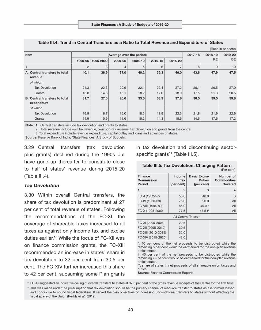
3.29 Central transfers (tax devolution

plus grants) declined during the 1990s but

have gone up thereafter to constitute close

to half of states’ revenue during 2015-20

(Table III.4).

Tax Devolution

3.30 Within overall Central transfers, the

share of tax devolution is predominant at 27

per cent of total revenue of states. Following

the recommendations of the FC-XI, the

coverage of shareable taxes increased to all

taxes as against only income tax and excise

duties earlier.10 While the focus of FC-XII was

on finance commission grants, the FC-XIII

recommended an increase in states’ share in

tax devolution to 32 per cent from 30.5 per

cent. The FC-XIV further increased this share

to 42 per cent, subsuming some Plan grants

in tax devolution and discontinuing sector-specific grants11 (Table III.5).

10 FC-XI suggested an indicative ceiling of overall transfers to states at 37.5 per cent of the gross revenue receipts of the Centre for the first time.11 This was made under the presumption that tax devolution should be the primary channel of resource transfer to states as it is formula based

and conducive to sound fiscal federalism. It served the twin objectives of increasing unconditional transfers to states without affecting the fiscal space of the Union (Reddy et al., 2019).

Table III.4: Trend in Central Transfers as a Ratio to Total Revenue and Expenditure of States(Ratio in per cent)

Item (Average over the period) 2017-18 2018-19 RE

2019-20 BE1990-95 1995-2000 2000-05 2005-10 2010-15 2015-20

1 2 3 4 5 6 7 8 9 10

A. Central transfers to total revenue

40.1 36.9 37.0 40.2 39.3 46.0 43.6 47.9 47.5

of which

Tax Devolution 21.3 22.3 20.9 22.1 22.4 27.2 26.1 26.5 27.0

Grants 18.8 14.6 16.1 18.2 17.0 18.9 17.5 21.3 20.5

B. Central transfers to total expenditure

31.7 27.6 26.6 33.6 33.3 37.8 36.5 39.5 39.8

of which

Tax Devolution 16.9 16.7 15.0 18.5 18.9 22.3 21.8 21.9 22.6

Grants 14.9 10.9 11.6 15.2 14.3 15.5 14.6 17.6 17.2

Note: 1. Central transfers include tax devloution and grants to states. 2. Total revenue include own tax revenue, own non-tax revenue, tax devolution and grants from the centre. 3. Total expenditure include revenue expenditure, capital outlay and loans and advances of states.Source: Reserve Bank of India, ‘State Finances: A Study of Budgets.

Table III.5: Tax Devolution: Changing Pattern(Per cent)

Finance Commission Period

Income Tax

(per cent)

Basic Excise Duties

(per cent)

Number of Commodities

Covered

1 2 3 4

FC -I (1952-57) 55.0 40.0 3

FC-IV (1966-69) 75.0 20.0 All

FC-VIII (1984-89) 85.0 45.0 * All

FC-X (1995-2000) 77.5 47.5 # All

All Central Taxes**

FC-XI (2000-2005) 29.5

FC-XII (2005-2010) 30.5

FC-XIII (2010-2015) 32.0

FC-XIV (2015-2020) 42.0

*: 40 per cent of the net proceeds to be distributed while the remaining 5 per cent would be earmarked for the non-plan revenue deficit states.#: 40 per cent of the net proceeds to be distributed while the remaining 7.5 per cent would be earmarked for the non-plan revenue deficit states.**: share of states in net proceeds of all shareable union taxes and duties.Source: Finance Commission Reports.


41

3.31 Although the FC-XIV increased tax devolution, it was essentially a compositional shift from tied to untied transfers12 (Reddy et al., 2019) (Chart III.13).

3.32 The levy of cesses and surcharges by the Union, which are outside the divisible pool, neutralises the increase in tax devolution

recommended by successive Finance

Commissions. The proceeds of cesses and

surcharges, which constituted only 2.3 per

cent of the gross tax revenue of the Centre

in 1980-81, has increased to 15 per cent in

recent years (Table III.6). The transition to GST

has seen the introduction of new cesses on

imports to make up for the cesses subsumed

under GST (Reddy et al., 2019). Although not

part of divisible pool, some part of this are

directed toward states’ welfare.

Grants and Loans

3.33 Grants constitute around 20 per

cent of the total revenue of states. Finance

Commission recommended grants account

for 18.7 per cent of total grants in 2018-19

(0.6 per cent of GDP). Notably, non-Finance

Commission grants, which constitute the

major portion at around 81.3 per cent of

total grants (2.6 per cent of GDP in 2018-19),

are routed through plan schemes and

12 Untied transfers are taken as tax devolution and portion of revenue deficit grant in FC grants, while tied transfers are FC grants excluding revenue deficit grants, non FC grants, and loans from the Centre.

Table III.6: Trend in Special Levies (Cess and Surcharges) by the Central Government (` crore)

Item 1980-81 1990-91 2000-01 2012-13 2013-14 2014-15 2015-16 2016-17 2017-18 2018-19 RE

2019-20 BE

1 2 3 4 5 6 7 8 9 10 11 12

1. Cess - - - 72,200 76,300 83,900 132,658 173,308 149,164 183,348 204,463

2. Surcharge - - - 19,500 28,000 31,900 39,053 44,537 54,151 142,672 164,648

3. Total Cess & Surcharge (1 + 2) 298 3,334 5,655 91,700 104,300 115,800 171,711 217,844 203,315 326,020 369,111

4. Centre’s Gross tax revenue (GTR) 13,149 57,576 188,603 1,036,200 1,138,700 1,244,900 1,455,648 1,715,822 1,919,009 2,248,175 2,461,195

5. Divisible pool 12,851 54,242 182,948 944,500 1,034,400 1,129,100 1,283,937 1,497,978 1,715,694 1,922,155 2,092,084

6. Share of Cess & Surcharge in Centre GTR (Per cent)

2.3 5.8 3.0 8.8 9.2 9.3 11.8 12.7 10.6 14.5 15.0

7. Devolution to States 3,790 14,241 50,737 291,500 318,200 337,800 506,193 608,000 673,006 761,454 809,133

8. States’ Share (Per cent) in Centre GTR

28.8 24.7 26.9 28.1 27.9 27.1 34.8 35.4 35.1 33.9 32.9

Note: ‘-’ NilSource: Report of the FC-XII and Union Budget, GoI, various issues.


42

Central Government Ministries for Centrally

Sponsored Schemes (CSS) and Central

sector schemes (Chart III.14).

3.34 Loans from the Centre to states, which is

the remaining component of transfers13, have

gradually come down with discontinuation

of Plan loans from the Centre since 2005-06

in line with the recommendations of FC-XII.

They constituted only 0.17 cent of GDP in

2018-19.

3.35 The current slowdown in the economy

is likely to have implications for tax devolution

to states. The corporate tax and GST rate cuts,

while are important to boost investment, may

result in revenue loss for states in 2019-20,

if not compensated by states’ own efforts

towards revenue mobilisation. As regards

grants, uncertainty with regard to the timing

and quantum of receiving the funds hinders

effective expenditure planning and utilisation

and is generally reflected in a tendency to over-

budget on the part of states14 (Refer Annex

in Chapter II). Adequate revenue to states

on this account and its productive usage is

crucial for achieving sustainable levels of debt

in the medium-term. It will help in reducing

their dependence on market borrowings and

address fiscal shocks on account of schemes

like UDAY or invocation of guarantees, if any,

as discussed in subsequent sections.

3. States’ Liability Burden: Power Distribution

3.36 State governments’ expenditure

on the power sector is largely in the form

of subsidies for agriculture and domestic

customer segments and loans and advances

13 Technically speaking, this component of transfers is a component of capital receipts of states, yet is covered under this section to complete the analysis of transfers.

14 As per states, along with uncertainty with regard to transfer dates, the criteria of transferring the funds to concerned departments within 15 days of receival prevents states from spending it effectively, with the actual expenditure remaining less than the budgeted expenditure.


43

to distribution companies (DISCOMs). At the same time, they benefit from revenue receipts from taxes and duties on electricity. For all states taken together, expenditure on power has always exceeded receipts from the sector. In states like Uttarakhand, Odisha, West Bengal, Gujarat, Himachal Pradesh, Sikkim, Chhattisgarh and Goa, however, the sector is a net contributor to the state exchequer (receipts exceed expenditure). Total power

sector expenditure by all states have shown a significant rise in 2003-04, 2015-16 and 2016-17, with UDAY and like schemes altering the composition of states’ spending in favour of capital expenditure15 (Chart III.15).

3.1 Power Distribution Utilities

3.37 Despite wide ranging reforms (Annex III), power distribution remains the weakest link in the sector’s value chain, weighed down

15 In restructuring programs, debt of utilities is taken over by the state either in the form of grants (revenue expenditure) or long-term financing of debt or equity (capital expenditure). In case of UDAY, DISCOMs’ debt was taken over largely in the form of state government debt initially (refer Box III.2) resulting in higher capital expenditure.


44

by consistent revenue gaps, bourgeoning losses and unsustainable debt levels. This, in turn, is impacting the upstream power generation companies that suffer from delays in payment of dues.

3.38 Historically, the financial performance of state-level power distribution utilities16 has suffered due to escalating costs and insufficient revenue mobilisation. On the cost side, power purchase cost (that occupies a dominant share in total cost) has increased significantly over the years, while the burden of interest expenses and personnel costs has been consistently high (Chart III.16 a and b).

On the revenue side, pricing by utilities is set below the actual cost for agricultural power and domestic (household) sectors in order to make power affordable for them, with the gap met through a combination of direct subsidy transfers and cross-subsidy from higher tariffs applied to industry. Utilities are unable to monetise the entire power supplied by them. Technical and commercial losses are high due to lack of investment in metering technology, infrastructure and theft (Chart III.16 c and d).

3.2 Impact of Power Distribution Restructuring

3.39 Financial restructuring of state power distribution utilities has been a regular feature

16 State Electricity Boards (SEBs) in the pre-unbundling era and Distribution Companies (DISCOMs) after the SEBs were unbundled into separate generation, transmission and distribution companies.


45

17 Under One Time Settlement (OTS) of 2003, the outstanding dues of State Electricity Boards (SEBs) to Central Power Sector Undertakings were securitised (power bonds with SLR status).

18 The Financial Restructuring Plan (FRP) of 2012, necessitated to enable DISCOMs to meet their short-term debt obligations, principally added to state governments’ outstanding guarantees in 2012-13 and 2013-14 as seven state governments – Andhra Pradesh, Punjab, Rajasthan, Uttar Pradesh, Haryana, Tamil Nadu and Bihar – guaranteed the issuance of bonds by DISCOMs to their lenders. Jharkhand conveyed its willingness to join the scheme but never came on board.

19 Press information bureau, November 05, 2015.20 Under UDAY, state governments are mandated to fund a progressively higher share of future DISCOM losses from their own finances. The

share of losses to be funded increases from 5 per cent in 2017-18 to 50 per cent by 2020-21.

in the past – One Time Settlement (OTS) in 2003; Financial Restructuring Plan (FRP) in 2012; and UDAY in 2015. These schemes significantly impacted state finances.

3.40 The OTS17 of 2003 caused deterioration in states’ debt position from 2003-04 till 2014-15. The FRP18 of 2012 expanded states’ outstanding guarantee liabilities without improving the financial performance of utilities. By 2014-2015, power distribution utilities had accumulated losses of ₹3.8 lakh crore and outstanding debt of ₹4.3 lakh crore, with banks reluctant to provide finance for additional losses19.

3.41 Under UDAY, which encompasses all states / union territories except West Bengal, Odisha and Delhi, the scope of debt

restructured was larger than under earlier programmes – state governments took over 75 per cent of outstanding liabilities of DISCOMs in the form of grants or equity. States that did not need debt restructuring were given the flexibility to enter into operational turnaround agreements. 16 states (including all the seven FRP states) signed comprehensive financial and operational turnaround agreements under the programme, which was funded through non-SLR UDAY bonds of `2.1 lakh crore. Finances of these states in the bond issuance years (2015-16 and 2016-17) were significantly impacted; interest payments, redemptions and DISCOMs’ loss funding20 continue to impact state finances on an ongoing basis (Chart III.17).


46

3.42 The performance of state DISCOMs exhibited significant improvement in reduction of revenue gaps by 2017-18, though some of the gains were reversed in 2018-19 by a sharp increase in power purchase cost. Overall by 2018-19, revenue gaps have reduced by 54 per cent from savings in interest cost, reduction in Aggregate Technical and Commercial (AT&C) losses, tariff hikes and revenue from grants (refer Box III.3). All 16 states have carried out tariff hikes since the start of the program, though the momentum of hikes has reduced from the initial years (Chart III.18).

3.43 Almost all states have registered an improvement in reducing the Average cost of supply – average realisable revenue (ACS-ARR gap) and in bringing down AT & C losses. However, they lag behind in eliminating the ACS-ARR gap and bringing AT & C losses to below 15 per cent by 2018-19 / 2019-20 as prescribed by the UDAY agreements (Chart III.19).

3.44 With the coupon rate on UDAY bonds at

a premium over those on SDL bonds, the cost

of debt servicing has gone up for the UDAY

states (Chart IV.20a). The impact on state

finances is likely to continue much beyond

the terminal year due to interest payment on

UDAY bonds and redemption of these bonds

(Chart IV.20b).

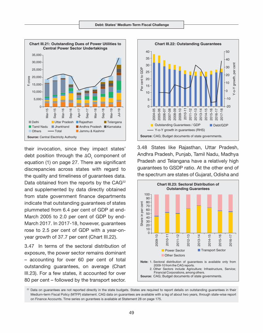
3.45 Outstanding dues of DISCOMs

towards power purchases have risen sharply

in the recent period, after registering decline

immediately post UDAY (Chart III.21). This

could be an indication of financial stress in

some DISCOMs, entailing the risk of fiscal

surprise from their future bailouts. Another

potential impact from UDAY could materialise

from takeover of incremental losses of

DISCOMs as mandated in UDAY agreements,

particularly as the benefit of grants to

supplement revenues will not be available for

some states (Box III.2).


47

4. Guarantees

3.46 State governments provide off-budget

support to State Public Sector Enterprises

(SPSEs) through guarantees21 on their

borrowings from financial institutions. While these guarantees help states undertake capital expenditure through the SPSEs, weak cost recovery mechanisms could render them a source of fiscal risk stemming from

21 Guarantees are different from off-budget liabilities that states undertake — where both interest and repayment are borne by the state government, though the borrowing is reflected in the books of SPSEs. There is limited information on these off-budget liabilities. Apart from guarantees issued to PSEs by state governments, these are also issued to municipal bodies, cooperative institutions, among others.


48

While the impact of UDAY on state finances from interest

payments and redemptions is predictable, the impact of future

losses takeover is inherently uncertain as it is dependent

upon the realised financial performance of DISCOMs. State

governments are mandated to fund a progressively greater

share of DISCOM future losses from their own finances and

prevent ballooning of losses on DISCOMs’ books. As per

this provision, states were supposed to provide funding of ₹

2,726 crore in 2018-19, though incomplete compliance with

this provision has resulted in less than half of this amount

being funded (Chart 1).

The impact of this provision on state finances could increase

significantly in 2019-20 and 2020-21 due to: i) higher share

of losses to be funded; and ii) reduction in revenue benefits

to DISCOMs from the conversion of state government debt

into grants on account of varied debt restructuring models

adopted by state governments.

Box III.2: Risks from Future Takeover of Losses under UDAY

The phased conversion of debt into equity or grant affects the

composition of state government expenditure and receipts

and impacts the revenue deficit (the gross fiscal deficit

and debt position are not impacted due to compensating

entries) (Chart 2a). The impact on DISCOMs’ financials is

also a factor as they will continue to hold a share of the debt

restructured till 2019-20, while generating revenue from

grants till 2020-21 (Chart 2b).

The reduction in revenue from grants for DISCOMs in

2018-19 to 2020-21 could potentially increase DISCOM

losses, particularly for states of Uttar Pradesh, Telangana,

Rajasthan, Jharkhand and Andhra Pradesh. This could

entail a significant fiscal outgo with a greater share of these

losses mandated to be funded by states. This makes it

incumbent upon states to take the necessary steps for the

turnaround of DISCOMs and to eliminate revenue gaps in a

time-bound manner.

Chart 1: DISCOMs’ Loss Takeover Schedule and Impact

Year Share of previous year’s DISCOM loss to be taken over by the state

2017-18 5 per cent

2018-19 10 per cent

2019-20 25 per cent

2020-21 50 per cent


49

their invocation, since they impact states’ debt position through the ∆Ot component of equation (1) on page 27. There are significant discrepancies across states with regard to the quality and timeliness of guarantees data. Data obtained from the reports by the CAG22

and supplemented by data directly obtained from state government finance departments indicate that outstanding guarantees of states plummeted from 6.4 per cent of GDP at end-March 2005 to 2.0 per cent of GDP by end-March 2017. In 2017-18, however, guarantees rose to 2.5 per cent of GDP with a year-on-year growth of 37.7 per cent (Chart III.22).

3.47 In terms of the sectoral distribution of exposure, the power sector remains dominant – accounting for over 60 per cent of total outstanding guarantees, on average (Chart III.23). For a few states, it accounted for over 80 per cent – followed by the transport sector.

3.48 States like Rajasthan, Uttar Pradesh, Andhra Pradesh, Punjab, Tamil Nadu, Madhya Pradesh and Telangana have a relatively high guarantees to GSDP ratio. At the other end of the spectrum are states of Gujarat, Odisha and

22 Data on guarantees are not reported directly in the state budgets. States are required to report details on outstanding guarantees in their Medium-term Fiscal Policy (MTFP) statement. CAG data on guarantees are available with a lag of about two years, through state-wise report on Finance Accounts. Time series on gurantees is avaliable at Statement 28 on page 175.


50

Uttarakhand. For states like Maharashtra, Bihar and Karnataka, guarantees are expanding in the recent period from relatively small initial levels (Chart III.24).

3.49 Measures have been put in place to safeguard against excessive reliance of SPSEs on guarantees and to ring-fence the state budgets from possible invocations. First, a guarantee fee is imposed by the state governments, varying from 0.5 per cent to 2.0 per cent of guarantees; however, it is often waived. Second, caps/limits are imposed by most states on issue of additional guarantees in the State Government Guarantees Act/Fiscal Responsibility Legislations (FRLs). Thirdly, as indicated in Chapter II, a few states have set up Guarantee Redemption Fund (GRF) for meeting the payment obligations as per FC-XII recommendation.

3.50 Although the outstanding guarantees are at modest levels at the current juncture, fiscally-stressed state governments may not have enough fiscal space to bear the

additional financial burden of invoked guarantees. Financing them via borrowings such as UDAY bonds may also have credit and financial market implications. A comprehensive framework for guarantee management is warranted with key elements including adherence to caps/limits based on sustainability, maintenance of GRF based on portfolio risk assessment by all states, timely collection of guarantee fees and comprehensive information on loans extended against state government guarantees/letters of comfort as also guarantees invoked and settled/waived-off.

5. Market Borrowings by States

3.51 In recent years, states’ financing mix has changed. In line with the recommendation of the FC-XIV, most of the states and union territories have been excluded from the National Small Savings Fund (NSSF) financing facility from 2016-17, increasing their reliance on market borrowing. Consequently, State Development Loans (SDLs) issuances have


51

picked up significantly in recent years with attendant liquidity risks, absence of credit risk sensitivity on yield differentials across states, a rise in redemption pressures and a narrow investor base.

5.1 Liquidity of SDLs

3.52 Out of 3,125 state government securities (including UDAY bonds) as on end-March 2019, only around 50 securities get traded. Liquidity is concentrated around few securities mostly closer to auction dates and it does not extend across the yield curve. The turnover ratio of SDLs is significantly lower than GoI securities and their share of trading volume in the secondary market remains miniscule as compared with the G-Secs market trading (Chart III.25).

3.53 The Working Group on Enhancing Liquidity in the Government Securities and Interest Rate Derivatives Markets (2012) (Chairman: Shri R. Gandhi) recommended the reissuance and consolidation of state development loans. Consequent upon the

Reserve Bank’s efforts, some states have gone for reissuances of their securities in recent years, which have improved liquidity in the secondary market (Box III.3).

5.2 Pricing of SDLs

3.54 There appears to be no observable relationship between borrowing spreads of SDLs and states’ fiscal health. The average inter-state spread stood at 6 bps during 2018-19 same as the year ago. This has resulted in symmetry in bidding patterns and states mobilising funds at similar or near similar yields for the same tenor SDLs, reflecting cross subsidisation between well managed states and others (RBI, 2018). Therefore, risk-based pricing of SDLs has the potential to reinforce self-discipline on states’ fiscal situation.

3.55 The RBI has been making various efforts to address the issue of lack of risk asymmetry in pricing of SDLs. In addition to weekly auctions of SDLs since October

2017, the RBI publishes monthly data on


52

Box III.3: Re-issuances of SDLs and Liquidity

Re-issuance of SDLs is a new phenomenon in the state

government security market, which may help in building

corpus for secondary market (volume) trading. It also

facilitates debt consolidation, albeit passive. Furthermore,

this may have a salutary impact on the yields in the

primary market and hence help in cost savings for the

government. During 2017-18 and 2018-19, seven states

undertook re-issuances. The volume of re-issued to total

issue of securities has gone up from 10.0 per cent in

2017-18 to 11.2 per cent in 2018-19. During 2017-18, the

average cut-off yield across all tenors of the re-issued

papers was 6.96 per cent as against average 7.15 per cent

of the non-reissued papers; likewise, the average cut-off

yield of re-issued papers across all tenors was 7.44 per

cent during 2018-19 as against 7.73 per cent for the non-

reissued securities.23

An ideal measure of the liquidity of the SDL market is the

bid-ask spread. However, due to low level of trading in

SDLs, other measures of illiquidity have been constructed,

viz., percentage of no trading days (PNT); Kyle Obizhaeva

(KO) and Amihud, following Amihud (2002) and Davis, et. al

(2018) (Table 1). The PNT is computed on the basis of the

number of non-trading days over the total trading days in a

month. The Kyle and Obizhaeva (KO) measure depicts the

variance of bond returns scaled by the volume traded. The

third measure of illiquidity, Amihud Illiquidity, takes into

account the return of the bond scaled by average volume

traded. The lower the value of these three measures of

illiquidity, better is the liquidity of a security.

PNTi,t = (Zero Volume Trading Daysi,t /Trading Days in

Montht)*100

Kyle Obizhaeva Illiquidityi,t = (Return Variance i,t /

Pricei,t*Volumei,t)1/3 * 106

Amihud Illiquidityi,t = (1/Di,t) * 106

where Di,t is the number of observations for security i during

time t

These measures of illiquidity indicate re-issued securities

are more liquid than non-reissued papers in respect of

5-year paper of Tamil Nadu and Maharashtra. However,

this relationship is not observed for shorter tenor securities.

(Contd.)

Table 1: Illiquidity Statistics of SDLs

2017-18 and 2018-19

Re-issued Non-reissued

State24 Tenor Volume (` Cr)

PNT KO Amihud Volume (` Cr)

PNT KO Amihud

Madhya Pradesh <1 1706 92.5 0.08 0.0000012 - - - -

Himachal Pradesh 3 97 95.49 1.67 0.006 - - - -

Maharashtra 3 602.03 91.8 1.52 0.001 1244.3 85.28 0.5326 0.0004

Maharashtra 5 3445.31 78.56 0.66 0.001 765.94 93.13 0.911 0.001

Tamil Nadu 5 2417.30 73.58 0.481 0.0005 635.51 90.06 1.27 0.00156

Maharashtra 10 10104.5 64.6 1.20 0.0103 2078.29 71.5 1.27 0.002

Tamil Nadu 10 8335.02 68.44 1.09 0.009 3314.81 70.76 1.25 0.009

Haryana 10 2642.42 71.19 1.21 0.003 1363.78 70.92 1.51 0.006

Punjab 10 5308.03 61.73 1.32 0.006 1450.39 75.01 2.07 0.026

Maharashtra 12 5832.37 67.93 1.7 0.016 - - - -

Punjab 12 2882.02 69.67 1.45 0.005 - - - -

Maharashtra 15 155 84.16 2.62 0.0035 - - - -

Punjab 15 2407.96 74.07 1.6 0.006 - - - -

Madhya Pradesh 15 939.71 81.69 2.23 0.0032 - - - -

-: not available.PNT- is calculated on an average.

23 Apart from re-issuance other factors such as tenor, macro economic conditions influence SDL yields.24 Odisha also re-issued a 19-year paper which is not considered for the analysis, due to unavailability of comparable paper.


53

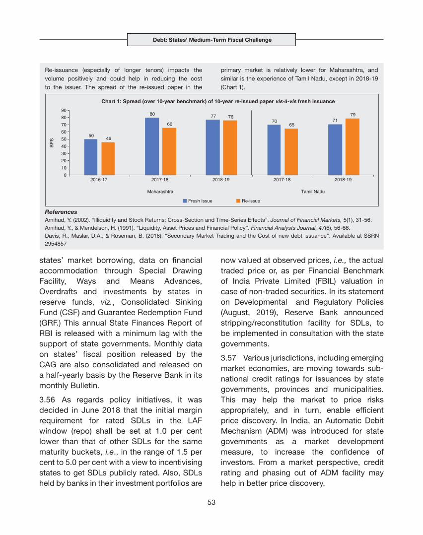
Re-issuance (especially of longer tenors) impacts the volume positively and could help in reducing the cost to the issuer. The spread of the re-issued paper in the

states’ market borrowing, data on financial accommodation through Special Drawing Facility, Ways and Means Advances, Overdrafts and investments by states in reserve funds, viz., Consolidated Sinking Fund (CSF) and Guarantee Redemption Fund (GRF.) This annual State Finances Report of RBI is released with a minimum lag with the support of state governments. Monthly data on states’ fiscal position released by the CAG are also consolidated and released on a half-yearly basis by the Reserve Bank in its monthly Bulletin.

3.56 As regards policy initiatives, it was decided in June 2018 that the initial margin requirement for rated SDLs in the LAF window (repo) shall be set at 1.0 per cent lower than that of other SDLs for the same maturity buckets, i.e., in the range of 1.5 per cent to 5.0 per cent with a view to incentivising states to get SDLs publicly rated. Also, SDLs held by banks in their investment portfolios are

now valued at observed prices, i.e., the actual traded price or, as per Financial Benchmark of India Private Limited (FBIL) valuation in case of non-traded securities. In its statement on Developmental and Regulatory Policies (August, 2019), Reserve Bank announced stripping/reconstitution facility for SDLs, to be implemented in consultation with the state governments.

3.57 Various jurisdictions, including emerging market economies, are moving towards sub-national credit ratings for issuances by state governments, provinces and municipalities. This may help the market to price risks appropriately, and in turn, enable efficient price discovery. In India, an Automatic Debit Mechanism (ADM) was introduced for state governments as a market development measure, to increase the confidence of investors. From a market perspective, credit rating and phasing out of ADM facility may help in better price discovery.

ReferencesAmihud, Y. (2002). “Illiquidity and Stock Returns: Cross-Section and Time-Series Effects”. Journal of Financial Markets, 5(1), 31-56.Amihud, Y., & Mendelson, H. (1991). “Liquidity, Asset Prices and Financial Policy”. Financial Analysts Journal, 47(6), 56-66.Davis, R., Maslar, D.A., & Roseman, B. (2018). “Secondary Market Trading and the Cost of new debt issuance”. Available at SSRN 2954857

primary market is relatively lower for Maharashtra, and similar is the experience of Tamil Nadu, except in 2018-19 (Chart 1).


54

5.3 Maturity Profile of SDLs

3.58 The maturity profile of borrowings by states is an important indicator of roll-over risks and debt servicing costs, which impinge on the efficacy of debt management strategies. In the aftermath of the global financial crisis (GFC), the market borrowing of states increased significantly, conditioned also by the cut-off of

access to NSSF funds. The bunching of the maturity profile of states borrowings around the ten-year bucket has also aggravated redemption pressures on states starting from 2018-19 and peaking in 2026-27 (as discussed in Chapter 2), warranting priority for strategies for elongation of maturities (Box III.4).

Box III.4: Elongation of Debt: Telangana ExperienceElongation of maturity of the portfolio is a preferred strategy in the cross-country experience to limit rollover risk in the debt structure, which has resulted in more resilient debt portfolios (OECD, 2019; Maravalle and Rawdanowicz, 2018; Chatterjee and Eyigungor, 2012). Long tenor bond issuance reduces refinancing risk, ‘locks in’ current yield levels in a rising interest rate scenario and creates benchmarks for valuation of long term corporate bonds, perpetual bonds and the present value of future income streams relating to long-term projects, especially in infrastructure. There are potential risks – uncertainty in pricing of long gilts; the possibility of locking in bonds at higher yields; and illiquidity of super-long gilts.

In India, the debt management has emphasised elongating the maturity profile of debt as a risk mitigation strategy. The maturity of Government of India’s outstanding borrowing has been steadily increasing, with the tenure of the longest

sovereign debt security being 40 years (GoI, 2018 and RBI, 2018). In contrast, market borrowing by state governments in India mainly relies mostly on issuance of ten-year bonds.

Since 2015-16, 15 state governments and the union territory of Puducherry have issued longer tenor securities. Among these states, the case of Telangana is instructive as the state has been issuing securities with longer tenors since 2016-17, with the longest tenor being 30 years (currently the longest tenor for state government securities). The effect of this strategy can be observed by comparing its actual redemption pattern vis-à-vis a hypothetical situation of issuance of standard 10-year securities only (Chart 1).

The maturity structure of Telangana debt profile has improved, with the weighted average maturity of market borrowings at 14.79 years at end-March 2019.

References:Chatterjee, S., & Eyigungor, B. (2012). “Maturity, Indebtedness, and Default Risk”. American Economic Review, 102(6), 2674-99.Government of India (2018). Status Paper on Government Debt for 2017-2018; Ministry of Finance, OECD. (2019). “Sovereign Borrowing Outlook for OECD Countries”. OECD Sovereign Borrowing Outlook 2019. OECD, Paris.Maravalle, A., & Rawdanowicz, L. (2018). “To shorten or to lengthen? Public Debt Management in the Low Interest Rate Environment”. OECD Economics Department Working Papers No 1483.Government of India (2018). Status Paper on Government Debt for 2017-18, Ministry of Finance. Reserve Bank of India (2018). Annual Report 2017-18.


55

5.4 Ownership Pattern of SDLs

3.59 The Indian SDL market remains largely

wholesale, dominated by public sector

banks and insurance companies which

account for about one-third each of SDLs

as on March 31, 2019, while provident

funds (PFs) account for about 22 per cent

(Chart III.26a). Recently, investments by

banks in SDLs have been declining in

line with the progressive reduction of

SLR requirements.25 In accordance with

the Medium-Term Framework (MTF) for

investment by Foreign Portfolio Investors

(FPIs) in Government securities put in place

since October 2015, the FPI limit prescribed

for SDLs is to be 2 per cent of the outstanding

stock of securities by the end of 2019-20. Of

this limit, i.e., ₹56,800 crore for both General

category and Long-term (valid till end-

September 2019) only 2.6 per cent has been

utilised till September 23, 2019. Moreover,

foreign investors have exited from states

SDLs which face deteriorating fiscal positions

(Chart III.26b).

3.60 The exposure of long-term FPIs

(sovereign wealth funds, pension funds, and

the like) in SDLs is nil. By contrast, FPIs have

shown ample appetite for Central government

securities as about two-thirds of limits on

them for general category FPIs stands utilised

as on September 23, 2019 (though long-term

FPIs have used only 30.6 per cent of their

limit).26 Improving transparency on states

fiscal positions is increasingly seen as a pre-

requisite for enhancing FPI interest in SDLs

(Table III.7).

25 Going forward, with the likely phasing out of ADM facility and reduction in SLR may impact the cost of borrowing for state governments and the attraction to hold SDLs in banks’ books, for reason other than the Yield to Maturity (YTM) they offer.

26 In fact, at end-March 2018, over 90 per cent of the total FPI limits in central government securities had been exhausted.


56

Table III.7: FPI in State Development Loans: Limits and Investment

End-March General Category Long-term FPIs Total

Upper limit (₹ crore)

Total Investment

(₹ crore)

Per cent of limits utilised


Total Investment

(₹ crore)



Total Investment

(₹ crore)


2014 - - - - - - - - -

2015 - - - - - - - - -

2016 7,000 4477 64.0 - - - 7,000 4477 64.0

2017 21,000 1560 7.4 - - - 21,000 1560 7.4

2018 31,500 5535 17.6 13,600 0 0.0 45,100 5535 12.3

2019 38,100 2468 6.5 7,100 0 0.0 45,200 2468 5.5

As on Sept. 23, 2019

49,700 1476 3.0 7100 56,800 1476 2.6

Memo item: Central government securities

As on Sept. 23, 2019

2,34,700 1,77,958 75.8 1,03,700 31,766 30.6 3,38,400 2,09,724 62.0

Note: “-: NIL”

3.61 The Reserve Bank has also been taking

various measures to widen the investor

base for SDLs. The endeavour to increase

the retail participation in the Government

security market is a case in point. In addition

to scheduled commercial banks and primary

dealers, specified stock exchanges approved

by SEBI have been permitted to act as

Aggregators/Facilitators (through a web-

based application provided to their clientele)

to submit consolidated bids under the non-

competitive segment of primary auctions.

In June 2019, it was decided to extend this

facility to the non-competitive segment of the

primary auctions of SDLs. The withdrawal of

some exemptions on the minimum residual

maturity requirement of FPI may also

contribute to widening the investor base of

SDLs.

6. Debt Sustainability

3.62 This section undertakes a

comprehensive debt sustainability analysis

for Indian States, both backward-looking

by using the trends in existing outstanding

liabilities of the states, and forward looking by

outlining the balance of risks as highlighted

in Sections 2 to 5 and keeping in mind the

recent growth slowdown.

3.63 The build-up of sub-national debt,

in reflection of the growing developmental

requirements of state governments and

their limited revenue raising capabilities, has

been aggravated in recent years by

restructuring schemes like UDAY as

discussed earlier in Section 3, and rise in

guarantees in Section 4. At moderate levels,

debt enhances economic growth while high

levels can put a drag on growth (Reinhart and

Rogoff, 2008; Checherita and Rother, 2010;

Woo and Kumar, 2010; Cecchetti, Mohanty

and Zampolli, 2011). As observed, states

with average debt to GDP ratios of more than

40 per cent in 2011-12 clocked lower growth

in the following three years, i.e., 2012-13 to


57

2014-15, while those with lower debt to GDP

ratio in 2011-12 witnessed higher growth over the same period (Chart III.27).

3.64 The evolving debt position of Indian states has witnessed several phases: a comfortable position prior to the Asian crisis of 1997, followed by a sharp deterioration till

2003-04. However, a significant improvement

occurred post the enactment of FRLs, only

to be derailed from 2015-16 by issuance

of UDAY bonds, farm loan waivers, and the

Seventh Pay Commission awards. The debt

to GDP ratio of states has risen to around 25

per cent, on an average, during the last three

years. Moving in tandem, the ratio of debt

to own revenue collections for states, was

edged to above 300 per cent since 2015-16.

(Chart III.28).

3.65 The FC-XIII, FC-XIV and the FRBM

Review Committee (Chairman: Shri N.K.

Singh) recommended debt targets for states.

In 2018-19 RE, while many states were below

the 3 per cent of GFD-GDP threshold, the

25 per cent debt to GDP threshold stands

breached by many states. A slightly stringent

criterion as prescribed by the FRBM Review

Committee and in line with the revised

FRBM implied debt target of 20 per cent will


58

put most of the states above the threshold

(Chart III.29).

3.66 India has the highest sub-national

debt vis-à-vis other BRICS countries

(Chart III.30). China stands at second highest,

mainly driven by rising local government

debt and the weak performance of public

corporations. If additional off-budget local government debt of 30 per cent to GDP is added for China, its sub-national debt would rise to over 50 per cent (IMF Fiscal Monitor, October 2018). The debt of other sub-nationals in countries like Colombia, Argentina and Indonesia, which borrow in the market by issuing state development bonds, remained subdued at less than 10 per cent of GDP.

3.67 Debt sustainability indicators assess the credit worthiness and the liquidity position of state governments by examining their ability to service interest payments and repay debt out of current and regular sources of revenue (excluding temporary or incidental revenue such as grants or capital receipts resulting from sale of assets). A declining ratio of interest payments to revenue receipts and a ratio less than 10 per cent (XIV-FC) is also regarded as indicative of debt being sustainable. An analysis on the indicators of


59

debt sustainability of states at aggregate level in different phases during the period 1981-82 to 2018-19 reveals that the real rate of interest has been lower than growth rate of real GDP in all phases, thus, fulfilling the necessary condition of debt sustainability. However, primary balance has remained consistently negative through all phases (except Phase III (2004-05 to 2007-08)), violating the sufficient condition of debt sustainability (Table III.8). Moreover, during the last phase (2015-16 to 2018-19) which coincides with the issuance of UDAY bonds, the highest primary deficit in the post-FRBM period has been recorded. Notwithstanding a decline in interest receipts to revenue receipts ratio, it has remained higher than the tolerable limit of 10 per cent as prescribed by FC-XIV. These developments signal potential debt sustainability risks.

3.68 In the literature, the measurement of debt sustainability27 has preferred backward looking empirical approaches with historical

Table III.8: States’ Debt Sustainability - Indicator-based Analysis

Phase I Phase II Phase III Phase IV Phase V Phase VI

Indicators 1992-93 to 1996-97

1997-98 to 2003-04

2004-05 to 2007-08

2008-09 to 2011-12

2012-13 to 2014-15

2015-16 to 2018-19

1 2 3 4 5 6 7

r*-g<0 -6.1 -1.0 -5.1 -10.1 -7.6 -4.4

PB/GDP ≥ 0 -0.8 -1.6 0.0 -0.6 -0.7 -1.3

IP/RR 15.6 22.4 19.1 13.8 12.1 11.9

D-G<0 -1.7 7.6 -4.8 -5.0 -2.0 3.4

*: Nominal interest rate is calculated as a ratio of interest payment at t to debt at t-1. CPI (IW) is used to derive real interest rate from nominal interest rate.Note: r is Real rate of interest; g is real output growth; PB is primary balance; IP is interest payments; RR is revenue receipts; D stands for rate of growth of public debt and G pertains to rate of growth of nominal GDP. Source: Budget documents of state governments and MoSPI.

information to evaluate the current debt position (Hamilton and Glavin, 1986; Trehan and Walsh, 1988; Bohn, 1998). In this tradition, a panel estimation capturing the heterogeneity across states and the downside risk of guarantees being invoked shows that for all states taken together, debt remains broadly sustainable in the medium-term, but becomes unsustainable when outstanding guarantees are incorporated into the debt stock (Box III.5).

3.69 Since the 1980s, EMEs have suffered frequent visitations of debt crises even as they engaged in progressive integration into the global economy either to harness new engines of growth or under the influence of IMF-driven structural adjustment programs. Quite naturally, debt sustainability analysis has moved to centre stage in the conduct of fiscal policy in these countries.

3.70 In view of the incidence of debt crises, practitioner approaches started overtaking the literature in proposing forward looking

27 Debt sustainability is a situation in which a borrower is expected to be able to service its debt without an unrealistically large future correction in the balance of income and expenditure (IMF, 2002).


60

Box III.5: Debt Sustainability of Indian States: An Empirical Assessment

The empirical literature on debt sustainability of Indian

States offers mixed evidence – debt is sustainable (Kaur

et. al 2018; and Renjith and Shanmugam, 2018) versus the

view that it is unsustainable (Shastri and Sahrawat, 2015;

Tiwari, 2012; Misra and Khundrakpam, 2009). Most of these

studies use the conventional outstanding liabilities concept

of debt to analyse its sustainability. The analysis presented

in this box contributes to the literature: first, by covering

all states28 in an updated time series including the post-

UDAY period for the first time and second, by going beyond

the conventional debt sustainability analysis to include

contingent liabilities in the form of guarantees under what is

termed as augmented debt, as recommended by XIV-FC, to

take a holistic approach of states’ debt sustainability.

Debt sustainability is analysed in a panel framework by

using a standardised approach (Bohn, 1998) that uses

historical information from the post-FRBM period 2004-05

to 2017-18 for all states29; encapsulated in a fiscal policy

response function as follows:

P i,t = αi + β di,t-1 + γ` Xi,t + εi,t ……. (1)

where P is the primary balance-to-GDP in year t; d is debt

stock in t-1 and X denotes control variables viz. output gap

and revenue receipts in this analysis. ‘β’ is the principal

coefficient which measures the response of the primary

balance to variations in debt. If a rising debt-to-GDP ratio

leads to a rise in the primary deficit, then debt tends to be

unsustainable which is reflected in a negative β coefficient.

A positive coefficient on the output gap indicates that

primary balance improves when GSDP is above trend.

While the other control variable — revenue receipts (RR)

— allows for differential fiscal structures amongst states as

some states have higher revenue generating capacity than

others. In this way, revenue receipts is representative of

stronger debt servicing capacity. All the variables have been

taken as proportions to GSDP. The estimations are carried

out with Feasible General Least Squares (FGLS) (Adams

et al., 2010; Abiad and Ostry, 2005), given the presence of

heteroscedasticity across states.30

Although the β coefficient is negative in Model 1, it is

insignificant, thus rejecting the null of unsustainability of

Table 1: Dependent Variable: Primary Balance as a

proportion to GSDP

Model 1 Model 2

Lag debt -0.02 (0.12)

Lag augmented debt -0.040***(0.00)

Real GSDP Gap 0.04* (0.06) 0.047**(0.03)

Revenue Receipts (RR) 0.06***(0.00) 0.07***(0.00)

Constant -0.58 (0.6) -1.25 (0.51)

Wald chi-squared (26) 302***(0.00) 320***(0.00)

Notes: 1. Figures in parentheses are p-values; ***, **,* significant at 1 per cent, 5 per cent and 10 per cent levels, respectively.

2. Augmented debt is obtained after adding outstanding guarantees to the outstanding liabilities of state governments. One-year lag of debt and augmented debt is taken to surmount the problem of endogeneity.

3. Cross-section and time-effects are taken into account.Source: Staff calculations

28 This is in line with the XIV Finance Commission analysis which eliminated the distinction between special category states and non-special category states.

29 For the above analysis, two states, viz. Goa and Jharkhand, have not been included in the estimation due to unavailability of data on the variable outstanding guarantees as augmented debt could not be calculated.

30 Breusch-Pagan test was carried out to check for heteroscedasticity and the null hypothesis of homoscedasticity was rejected.

states’ debt. In Model 2, however, which considers the

unlikely scenario of invocation of all states’ guarantees

(augmented debt in Table 1), the β coefficient is negative and

significant at 1 per cent level, and debt clearly moves into

the unsustainable zone. The control variables are correctly

signed and are statistically significant. Robustness checks

have been conducted by using other control variables, viz.,

revenue receipt gap and primary expenditure gap and they

buttress the empirical results.

This analysis highlights the vulnerability of states’ debt to

guarantees, if invoked. On balance sheet accumulation

of debt, it does not pose imminent risks at this juncture,

although the quality of spending by states and improving

tax buoyancies are key to attaining the FRBM debt targets.

References

Abiad, A. d., & Ostry, J. D. (2005). “Primary Surpluses and

Sustainable Debt Levels in Emerging Market Countries”.

IMF Policy Discussion Papers, 05(6).

Bohn, H. (1998, Aug). “The Behavior of U.S. Public Debt and

Deficits”. Quarterly Journal of Economics, 113(3), 949-963.

Kaur, B., Mukherjee, A., & Ekka, A. P. (2018). “Debt

Sustainability of States in India: An Assessment”. Indian

Economic Review, 53(1), 93-129.


61

approaches to debt sustainability, both external and fiscal. They provided more realistic assessments of the future rather than the past and the current, and this caught the attention of policy authorities across the world. Various country experiences with managing debt sustainably eventually crystallised into the Debt Sustainability Analysis (DSA) framework of the IMF (2002) and the World Bank (2005) with small variations by other multilateral agencies (OECD, 2013; ECB, 2011).

3.71 At the core of the DSA is the historical decomposition of debt dynamics and the baseline scenario projected over a minimum duration of five years. Standardised DSA templates, stress testing and risk scenarios around the baseline projection came to be recommended by the IMF- World Bank for wide country adoption (IMF 2008; World Bank 2006).31 Improvements were made in the template by streamlining the DSA with the use of simplified tables focusing on the baseline and the historical scenarios. Furthermore, considering that there is a tendency for policymakers to be optimistic in their projections, realism in formulating medium-term fiscal projections is envisaged in spelling out the assumptions and a periodic review of them is crucial (IMF, 2002).

3.72 In a conventional DSA, debt accumulation is driven by two main factors: i) the primary balance; ii) the differential between the interest rate and GDP growth rate. The path of debt can be expressed in an accounting-based approach linked to the inter-temporal

budget constraint as follows (Buiter, 1985;

Blanchard 1990):

dt = dt-1(1+rt)/(1+gt) - pbt ……. (1)

From equation (1), the dynamic debt

accumulation equation follows as:

dt = dt-1(rt - gt)/ (1+gt) - pbt ……. (2)

where dt is the ratio of debt to GDP, rt is the

nominal interest rate, gt is the nominal GDP

growth rate and pbt is the ratio of primary

balance to GDP at time t.

3.73 As per equation (2), a stable or declining

debt ratio (i.e. ∆dt ≤ 0) can be achieved even

with primary deficits if the same is offset by

a sufficiently large negative interest-growth

differential (rt - gt). This dynamic nature of debt

accumulation is encapsulated in the forward-

looking projection of the medium-term

debt-to-GDP ratio and the ratio of primary

balance-to-GDP that can stabilise the debt-

to-GDP ratio (IMF, 2003; IMF, 2013).

3.74 The IMF Article IV Consultations report

for India presents results of the DSA for the

general government. In this chapter, a DSA

is undertaken exclusively for states for the

first time. This analysis provides a likely time

path for debt till 2024-25, the terminal year

of achieving the revised FRBM debt target,

thus, providing forward guidance to States,

albeit in a consolidated format.

3.75 The key underlying assumptions for

the baseline projections for all states taken

together are set out in Table III.9.31 Beyond this, the template performs sensitivity tests to key parameters – interest rate, GDP growth, inflation, the exchange rate and the primary

balance.


62

Table III.10: Debt Sustainability Analysis- Key Assumption and Results Per cent

Variable Historical data Projections

2014-15

2015-16

2016-17

2017-18

2018-19

Last 5 years

average

2019-20

2020-21

2021-22

2022-23

2023-24

2024-25

Average for the

projection period

Key assumptions

1. Real GDP growth 7.4 8.0 8.2 7.2 6.8 7.5 6.9 7.5 7.7 7.7 7.7 7.7 7.5

2. Inflation / GDP deflator Y-o-Y change 3.3 2.3 3.1 3.8 4.1 3.3 3.8 4.0 4.0 4.0 4.0 4.0 4.0

3. States primary deficit excluding UDAY 1.3 1.0 1.3 0.8 0.7 1.0 0.7 0.6 0.6 0.5 0.5 0.5 0.6

4. Weighted average interest rate 7.8 8.0 7.9 7.7 7.4 7.8 7.4 7.0 7.0 7.1 7.1 7.1 7.1

Key results for the baseline scenario

Debt to GDP ratio in the baseline scenario 21.7 23.4 24.8 25.1 24.8 24.0 24.8 24.4 24.0 23.4 22.8 22.3 23.6

Gross Financing Needs 4.0 3.7 4.2 3.9 3.9 3.9 3.0 2.8 2.8 2.7 2.6 2.6 2.7

Guarantees invoked / future bailouts scenario 25.8 26.4 25.9 25.2 24.6 23.9 25.3

Gross Financing Needs 4.0 3.7 4.2 3.9 3.9 3.9 4.0 3.8 2.9 2.8 2.7 2.7 3.1

Assumed liability from guarantees / bailouts 1.0 1.0 0.0 0.0 0.0 0.0 0.3

Note: 1. Gross Financing Needs = Primary Deficit + Net Interest Payments + Amortisation Payments for Existing Debt. 2. Primary Deficit is calculated as per IMF DSA methodology, i.e. primary receipts exclude interest receipts.Source: Staff estimates.

3.76 In the forward-looking path for the debt-GDP ratio in the baseline scenario, it is projected to decline to 22.0 per cent by 2024-25. The key downside risk to the baseline projections is a lower than assumed GDP growth and/or crystallisation of potential off-budget liabilities in the form of guarantees. A scenario whereby the impact of the latter

is assumed to be 2 per cent of GDP (impact

from UDAY was 1.4 per cent of GDP), spread

across 2019-20 and 2020-21 causes the

debt-GDP ratio to go up to about 24 per cent

by 2024-25 (Table III.10, Chart III.31).

3.77 The decline in debt-to-GDP ratio is

driven by the interest-growth differential

Table III.9: Key Assumption for States DSA Model

Variable Assumptions

Primary Balance Primary receipts are assumed to move with nominal GDP growth with an average buoyancy of 1.1 during the projection period.

Primary expenditure growth has been assumed to grow at a constant rate, based on the average of 2014-15 and 2018-19 (adjusting for the one-time impact of UDAY).

Accordingly, there is a reduction in primary deficit from 0.7 per cent of GDP in 2018-19 to 0.5 per cent of GDP in 2024-25

GDP growth The RBI’s GDP growth projection is assumed for 2019-20 and the IMF’s projections for India are taken for the remaining period.

Inflation Assumed at 4 per cent, in line with the inflation target.

Weighted average interest rate Calculated as interest payments divided by debt stock (excluding guarantees) at the end of the previous year (new borrowings to be undertaken at the rate for 2018-19).

Source: Staff estimates; and World Economic Outlook, IMF, April 2019.


63

which is partially offset by the primary deficits

being lower than the debt stabilising level

of 1.0 per cent of GDP. The interest-growth

differential has been negative in India for

the past 16 years, leaving space for running

primary deficits.

3.78 In both our baseline projection and

downside scenario of guarantees being

invoked, the level of debt-GDP ratio in

2024-25 is higher than the revised FRBM

target of 20 per cent but below the 25 per

cent debt ceiling imposed by the FC-XIV.

However, the invocation of guarantees

causes the states to breach the 25 per cent

ceiling in the years of 2019-20 to 2022-23.

For achievement of FRBM target of 20 per

cent debt-GDP ratio by 2024-25, states will

have to grow their receipts by about 14 per

cent year-on-year. This can only be achieved

through higher GDP growth and/or improved

tax buoyancy.

7. Concluding Observations

3.79 In the Indian fiscal landscape, states are entrusted with higher responsibilities but less than commensurate resources. On the revenue front, states might see a crunch because of the economic slowdown, though they remain protected against any own shortfall in GST collection by compensation cess.

3.80 On the expenditure front, schemes like farm loan waivers and UDAY, which are essentially in the nature of fiscal shocks, have kept spending pressures high. What is worrisome is that they are associated with spiralling states’ market borrowings with implications for states’ outstanding debt. Analysis in this chapter points to still pending medium-term risk in the form of higher losses of DISCOMs falling onto state budgets. In addition, rising state government guarantees also pose a medium-term fiscal challenge for states.

3.81 While market borrowings by state governments have risen significantly, a combination of consolidation, reissuances and maturity elongation can help in improving liquidity, and in developing a secondary market with a diversified investor base comprising institutional investors, multilateral financial institutions and foreign portfolio investors with considerable promise of throwing up the desired differential pricing and market disciplining among states.

3.82 The debt position of state governments has deteriorated post-UDAY though still remains sustainable, but vulnerable to potential risks with invocation of states’


64

guarantees. Going forward, fiscal readjustments to boost growth without accumulating public debt may warrant improvement in spending for infrastructure and the social sector, given the high capital expenditure multiplier. States will have to improve tax buoyancy by capitalising on the efficiency gains under the GST and digitisation,

and by exploiting the scope for raising user charges wherever possible so as to improve their revenue raising capacity and reduce reliance on borrowings. Addressing these issues give states the wherewithal to support growth by not curtailing desired expenditure and hence, maintaining sustainability in the long-run.


65

Annex III.1Evolving Institutional Mechanism for GST

GST was enacted with the Constitution (One

Hundred and First Amendment) Act, 2016, giving

way to the Central Goods and Services Tax

(CGST), State Goods and Services Tax (SGST),

Integrated Goods and Services Tax (IGST) and

the Compensation Law. The Act amended the

articles 248, 249, 250, 268, 269, 270, 271, 286,

366 and 368 along with the Sixth and Seventh

Schedules of the Constitution. Also, Article 268A

was omitted while new articles 246A (Special

provision with respect to goods and services tax),

269A (Levy and collection of goods and services

tax in course of inter-State trade or commerce)

and 279A (Goods and Services Tax Council) were

inserted in the Indian Constitution.

The Goods and Services Tax Network (GSTN)

has been set up to provide IT infrastructure and

services to the Central and State Governments,

tax payers and other stakeholders for flawless

implementation and filing of GST. It is a

non-Government, private limited company

under Section 8 of the new companies Act

with authorised capital of `10 crore. It was

incorporated on March 28, 2013. The Government

of India holds 24.5 per cent equity in GSTN and

all states, including Delhi and Puducherry, along

with the Empowered Committee (EC) of State

Finance Ministers, together hold another 24.5

per cent. The balance 51 per cent equity is held

by non-Government financial institutions (Goods

and Services Tax Network).

The GST Council is responsible for the entire

architecture of GST as there is no exclusive tax

base for the Union or states. Being a credible

institution promoting cooperative federalism,

decision making in the GST Council also reflects

the wisdom of both the Centre and states (Reddy

et. al, 2019).

The four Acts that govern the GST architecture

are the CGST Act, SGST Act, IGST Act and the

GST (Compensation to States) Act. The Centre

levies and collects CGST (governed by the CGST

Act), the states would levy and collect SGST

on all transactions within their geographical

boundaries (governed by the SGST Act). Input

tax credits (ITC) under the CGST and the SGST

are available for discharging the liability on the

output at each stage without cross utilisation

of credit. The IGST (governed by the IGST Act)

is levied on all imports into the territory of India

as well as on the inter-state supply of goods or

services or both. It is collected by the Centre and

distributed between the Centre and states. The

states are entitled to receive a compensation to

the tune of the difference between the projected

revenue based on 14 per cent annual growth

over the base year 2015-16 and the actual

revenue. The compensation has to be provided

for a period of five years, viz., 2017-2022 (GST

(Compensation to States) Act).

These Acts have been amended from time to

time in order to deal with practical difficulties

thrown up by actual experience. One of the major

amendments has been with respect to the IGST

apportionment. As per the IGST Act, 2017, the

apportionment of the IGST collection was based

on the principle of first place of landing, viz.,

IGST would be apportioned to states where the

actual supply of goods takes place and to the

Centre where the supply takes place in a Union


66

Territory. The balance amount (which cannot

be apportioned clearly based on these criteria)

was parked in the Consolidated Fund of India

(CFI) and apportioned on the basis of the FC-XIV

devolution rule of 42 per cent to the states (done

in the months of February and July 2018 as per

data provided by the Office of the Controller

General Of Accounts), with the remaining

accruing to the Centre. In order to eliminate

discrepancies in apportionment to the States,

the IGST Act was amended with effect from

August 2018, whereby “…the balance amount,

for the time being, on the recommendations

of the GST Council, will be apportioned at the

rate of 50 per cent to the Central Government

(as part of CGST) and 50 per cent to the State

Governments or the Union territories, (as part of

SGST or UTGST, respectively) as the case may

be, on ad-hoc basis…..” (IGST (Amendment) Act,

2018).

Apart from amendments, measures undertaken

by the GST council have aimed at streamlining

input tax credits and e-way bill system (details in

Annex III.2).

References

Central Board of Indirect Taxes and Customs: www.cbic.gov.in

CGST Act, SGST Act, IGST Act and GST (Compensation to States) Act

Goods and Services Tax Network: www.gstn.org

IGST (Amendment) Act, 2018

Reddy, Y. V., & Reddy, G. R. (2019). “Indian Fiscal Federalism”. Oxford University Press.


67

Date Event Major Decisions

September 15, 2016

Constitution of the GST Council

• Vide F. No. 31011/09/2015-SO (ST) dated 15th September, 2016, the President of India constituted the “GST Council”.

• GST Council can hold meetings and take decisions on various major issues such as Model law, rate of taxes, exemptions etc.

September 16, 2016

Enactment of GST Amendment Act.

• By Ministry of Finance’ vide Notification No. S.O. 2986(E) dated September 16, 2016, all sections of Constitution (One Hundred and First Amendment) Act, 2016 came into force.

GST Council Meeting

September 22, 2016

First • Threshold exemption limit decided at `10 Lakhs for North-Eastern states and `20 Lakhs for the rest of India.

• States will have sole jurisdiction over assessees having a turnover of `1.5 crores or less. The existing service tax assessees will continue to be under jurisdiction of Centre.

• The Centre will pay quarterly or bi-monthly compensation to states, in case of any revenue loss.

• Decided 2015-16 as the base year for calculating the compensation.

September 30, 2016

Second • The GST Council finalised five subordinate legislations relating to payment, returns, refunds, invoice and registration.

• Consensus on area-based exemption in accordance with those granted under the current excise regime.

• Taxes will have to be collected and it can be reimbursed from the annual budgets to the exempted categories.

• To compensate states for 5 years for loss of revenue due to implementation of GST, the base year for the revenue of the state would be 2015-16 and a fixed growth rate of 14 per cent will be applied to it.

October 19, 2016

Third • Proposed a four-tier rate structure comprising a lower rate of 6 per cent, two standard rates of 12 per cent and 18 per cent and a higher rate of 26 per cent with an additional cess for luxury and demerit goods.

• Cess was proposed to be used for payment of compensation to the states. However, consensus could not be reached.

Annex III.2 Timeline of GST Council Meetings and Major Decisions


68

November 3, 2016

Fourth • Decided a four-tier GST rate structure of 5 per cent, 12 per cent, 18 per cent and 28 per cent.

• Essential items including food will be taxed at zero rate.

• The lowest rate of 5 per cent would be for common use items.

• 12 per cent and 18 per cent would be the standard rates.

• The highest rate would apply to luxury and de-merit goods, which will also attract an additional cess.

• The collection from this cess as well as clean energy cess will be used for compensating states for any loss of revenue during the first five years of implementation of GST.

December 2-3, 2016

Fifth • Consensus could not be reached on the issue of sharing of administrative powers between the centre and the states.

December 11, 2016

Sixth • The Council discussed on the Model CGST and SGST legislation (Model GST Law) which was released in the public domain on November 26, 2017.

• Could not reach on consensus on issue of dual control of assesses.

December 22-23, 2016

Seventh • Draft CGST and SGST laws were cleared along with compensation law.

• No consensus was reached on issue of dual control.

January 3-4, 2017

Eighth • Issue of dual control remained unresolved.

• States raised a new issue of split in tax rate in ratio of 60:40 between states and Centre instead of equally dividing GST between Centre and states.

• States demanded taxation rights for sales made in the high seas within 12 nautical miles.

• States requested to increase the number of items on which this new Cess is to be levied.

January 16, 2017

Ninth • A broad consensus for GST to be rolled out from 1st July 2017, instead of 1st April 2017 was made.

• The issue of dual control was broadly resolved. States will have powers to assess and administer 90 per cent of the tax payers under `1.5 crores annual turnover while the remaining 10 per cent would be controlled by the Centre.

• Tax payers with turnover more than `1.5 crores will be controlled and administered in 50:50 ratio both by State and Centre.

• States can levy GST within 12 nautical miles.

• Any IGST disputes among states will be resolved by the Centre.


69

February 18, 2017

Tenth • Formally approved Compensation law.

• Some of the issues in three crucial draft CGST/SGT/IGST laws were discussed.

March 4, 2017

Eleventh • Council cleared the two key draft laws of Central GST (CGST) and Integrated GST (IGST).

• Hotels with annual turnover of less than `50 lakhs, will pay the lowest tax rate of 5 per cent under the GST regime.

March 16, 2017

Twelfth • Cleared the remaining two supplementary legislations UTGST (Union Territory GST Law) and the SGST (State GST Law) needed for implementation of the goods and service tax (GST) regime.

• Approved the bound rate of 15 per cent as peak rate for the proposed Cess to be levied on certain demerit goods.

March 31, 2017

Thirteenth • Approved the Rules relating to Input Tax Credit, Valuation, Composition and Transition.

• Gave final approval for changes in rules for filing tax returns in the new regime, registration of entities, payment of GST, invoicing and refunds to make them compatible with GST laws.

May 18-19, 2017

Fourteenth • Fitment of rates were discussed. The council approved the GST rate of goods at nil, 5 per cent, 12 per cent, 18 per cent and 28 per cent levied on certain goods. It also approved the rates for GST compensation cess to be levied on certain goods.

• Constitution of eighteen sectoral groups to ensure smooth roll-out of GST.

June 03, 2017

Fifteenth • Clearance of pending Transition and Returns rules.

• Tax rates on gold, textiles, trademarked packaged items, solar panels, biscuits and footwears were decided.

June 11, 2017

Sixteenth • Approval of amendments to draft GST rules.

• Rates on 66 items reduced including movie tickets, packaged food and cashew nuts among others.

• Increase in turnover limit for composition scheme.

• Exemptions on few supply of services.

June 18, 2017

Seventeenth • Announcement of official roll out on July 01, 2017.

• For the first two months of implementation, tax would be payable based on a simple return (Form-GSTR-3B) containing summary of outward and inward supplies which will be submitted before 20th of the succeeding month.

• Regular GSTR-1 to be filed for July-August 2017.

• No late fees and penalties for the interim period.


70

• 28 per cent limit on hotels start from `7500 per unit per day; 18 per cent for hotels between `2500 to `7500 per unit per day.

• State run lotteries taxed at 12 per cent.

• IGST of 5 per cent on Ship with full ITC applicable.

• 6 rules were cleared inclusive of anti-profiteering.

June 30, 2017

Eighteenth • Tax rate on fertilizers reduced to 5 per cent from previously decided 12 per cent.

• Rate on exclusive parts of tractors cut to 18 per cent from 28 per cent.

July 17, 2017

Nineteenth • Increase in compensation cess rates on cigarettes.

August 5, 2017

Twentieth • Final drafting of e-way bills.

• Job work of all kinds of textiles to be taxed at 5 per cent.

• Rates on tractor parts brought down to 18 per cent.

• Government given work contracts like roads bridges canals to be taxed at 12 per cent with credits from 18 per cent earlier.

• Anti-profiteering mechanism to get started by appointing state-wise committees.

• GST rates for certain services revised downwards and few services given exemption.

• Option given to certain services for GST rates and clarification provided for GST on few services.

September 9, 2017

Twenty-first • Revised schedule for filing GST returns to facilitate taxpayers.

• GSTR-3B to be continued for August-December 2017.

• Option for composition scheme to registered person who had not opted for it earlier.

• Committee set up consisting of officers from both the Centre and the states under the chairmanship of Revenue secretary to examine issues related to exports.

• Group of Ministers constituted to monitor and resolve the IT challenges faced during GST implementation.

• Registration of persons liable to deduct TDS and collect TCS will commence from September 18, 2017.

• Due date for submission of FORM GST TRAN-1.


71

October 6, 2017

Twenty-second • Facilitative changes to ease the burden of compliance on small and medium businesses inclusive of the following major measures:

(i) changes in composition scheme

(ii) relief from registration for service providers with annual turnover of less than `20 lacs

(iii) ease of payment and return filing

(iv) relief from reverse charge mechanism till March 31, 2018

(v) e-way bill system to be introduced in a staggered manner from April 1, 2018

(vi) extension to filing of FORM GSTR-4 under composition scheme

(vii) modification of invoice rules

(viii) GST to be paid at the time of supply of goods and not earlier by taxpayers with aggregate turnover up to `1.5 crores.

November 10, 2017

Twenty-third • Major rationalisation of rates on certain goods and services across many sectors.

• Further simplification of return filing.

• Extension of dates for filing returns.

• Exporters exporting services to Nepal and Bhutan eligible for claiming input tax credit in respect of goods and services used for effecting such exempt supply of services to Nepal and Bhutan

• All service providers supplying intra-State, inter-State or through e-commerce operator exempt from obtaining GST registration if their aggregate turnover does not exceed `20 lakhs.

• Benefits for Diplomatic/UN Missions.

December 16, 2017

Twenty-fourth • Nationwide e-way bill system to be ready by January 16, 2018.

• Uniform system of e-way bill for inter-State and intra-State movement to be implemented by June 1, 2018.

January 18, 2018

Twenty-fifth • Second set of major relief measures regarding GST rates on goods and services covering many sectors and commodities.

• Issuance of certain clarifications on issues relating to GST rates and taxability of certain goods and services.

• Policy changes related to late fee, cancellation of registration, filing FORM GST REG-29, modification to e-way bill rules.


72

March 10, 2018

Twenty-sixth • Extension of tax exemption on imported goods to exporters availing various export promotion schemes for six months.

• Creation of E-Wallet Scheme.

• Review of progress made in grant of refunds to exports of both IGST and input tax credit.

• Liability to pay tax on reverse charge basis deferred till June 30, 2018.

• TDS/TCS suspended till June 30, 2018.

• Improvements in e-way bill rules.

• GST implementation committee tasked with grievance redressal to taxpayers regarding IT glitches.

• Recommendations regarding data analytics.

May 04, 2018

Twenty-seventh • Incentive to promote digital transactions.

• Imposition of sugar cess over and above 5 per cent GST and reduction in GST rate on ethanol.

• Approval of principles for filing of new return design based on recommendations of the Group of Ministers on IT simplification.

July 21, 2018

Twenty-eighth • Amendments to CGST Act, 2017, IGST Act, 2017, UTGST Act 2017 and GST (Compensation to states) Act, 2017.

• Approval of simplified GST return formats and associated changes in law.

• Major rationalisation of rates of several goods including specified handicraft items.

• Decisions relating to exemptions / changes in GST rates / ITC eligibility criteria, rationalisation of rates/ exemptions and clarification on levy of GST on services.

August 4, 2018

Twenty-ninth • Formation of Group of Ministers to examine MSME related issues.

• GST concessions on digital payments.

September 28, 2018

Thirtieth • Formation of Group of Ministers to look into imposition of cess under GST to provide relief to Kerala flood victims and a temporary tax under GST to help states in exigencies among few other issues relating to natural calamities.

• A panel of analysts to conduct research on all states pertaining to GST collection and recommend ways to bridge the gap between the current revenue and targeted revenue.

December 22, 2018

Thirty first • Major change in rates of goods and services across sectors.

• 7 member Group of Ministers formed to study the revenue trend, including analysing reasons for structural patterns affecting the revenue collection in some states.


73

January 10, 2019

Thirty-second • Approval for changes made by CGST (Amendment) Act 2018, IGST (Amendment) Act, 2018, UTGST (Amendment) Act 2018 and GST (Compensation to States) Amendment Act, 2018 along with amendments in CGST Rules, notifications and circulars issued earlier and corresponding changes in SGST Acts to be notified with effect from January 02, 2019.

• Last date for passing the examination for GST practitioners (who have enrolled under rule 83(1)(b)) to be extended till December 31, 2019.

• Relief to MSME (including small traders).

February 24, 2019

Thirty-third • Several measures were announced to boost the residential segment of the real estate sector.

March 19, 2019

Thirty-fourth • Modalities for transition to lower effective GST rate of 1 per cent in case of affordable houses and 5 per cent on construction of houses other than affordable house (as recommended in 33rd meeting).

• Amendment to input tax credit rules.

June 21, 2019

Thirty-fifth • New return system to be introduced in a phased manner.

• Extension regarding furnishing returns under various Forms.

• Issues placed before Fitment committee regarding GST on electric vehicles and solar power generating systems and wind turbines.

• Report on Lottery submitted by Group of Ministers.

• Extension of tenure of National Anti-Profiteering committee by two years.

• Location of benches of the State and the Area Benches for the Goods and Services Tax Appellate Tribunal (GSTAT) for various states and Union Territories.

• Electronic invoicing system to be introduced ina phased manner.

July 27, 2019

Thirty-sixth • GST rate on all Electric Vehicles reduced from 12 per cent to 5 per cent and of charger or charging stations for EVs from 18 per cent to 5 per cent.

• Hiring of electric buses by local authorities exempted from GST.

• Date extended for filing of intimation in FORM GST CMP-02 for availing the option of payment of tax under notification No. 2/2019-Central Tax (Rate) dated 07.03.2019 (by exclusive supplier of services).

• Date extended for furnishing statement containing the details of the self-assessed tax in FORM GST CMP-08 for the quarter April, 2019 to June, 2019 (by taxpayers under composition scheme).


74

September 20, 2019

Thirty-seventh • Rationing of GST rates on hotel accomodations across various categories, outdoor catering services.

• Reduction in compensation cess on passenger vehicles.

• Simplification of forms for annual return and reconciliation statement to be examined.

• Introduction of new return system from April 2020.

• Linking of Aadhaar with registration of tax-payers and examining the possibility of making Aadhaar mandatory for claiming refunds.

Source: http://www.gstindiaonline.com/ ; https://gstindiaguide.com/gst-council-finalise-draft-rules-today/; http://www.cbic.gov.in/htdocs-cbec/gst/index; pib.nic.in


75

Annex III.3 Power Distribution – the History of Reforms and Government Programmes

Historically, the growth in power sector in India which began in the private sector, underwent a major shift post the passage of the Industrial Policy Resolution of 1956, which reserved generation and distribution of electricity exclusively for the public sector. Power sector is a concurrent subject under Article 246 of the Indian Constitution, and states came to play the pivotal role following the passage of the Electricity Supply Act 1948 (ESA) that mandated the setting up of State Electricity Boards (SEBs). SEBs were constituted as vertically integrated entities covering generation, transmission and distribution of power. Power distribution was exclusively the domain of SEBs, while Central government played a role in generation and transmission of power.

The first attempt to liberalise the power sector was made with an amendment to the ESA in 1991 that allowed for private sector participation in power generation, though power distribution continued to remain the province of SEBs. Reforms in power distribution have their beginnings at state-level, with Odisha becoming the first state to restructure its SEB with the support of World Bank. The ‘Odisha Model’ for reforms as it came to be called involved restructuring of the SEB into separate generation, transmission and distribution entities. Specifically, the distribution segment of the Orissa State Electricity Board (OSEB) was divided into four regional utilities and later privatised. The ‘Odisha Model’ was adopted by states of Haryana (1997), Andhra Pradesh (1998), Uttar Pradesh (1999), Karnataka (1999), Rajasthan (1999), Delhi (2000), Madhya Pradesh (2000) and Gujarat (2003). Each of these states unbundled their SEBs into separate generation,

transmission and distribution. However, unlike Orissa and Delhi that went a step further and privatised their distribution companies, all other states retained ownership of the unbundled distribution company.

The period of 1998-2003 is characterised by wide ranging reforms in the power sector to address the financial problems of the distribution sector. A key reason identified for distress in the distribution sector was low electricity tariffs due to associated political economy and public utility pricing. With a view to establishing a robust mechanism to ensure that electricity tariffs are set according to economic principles, the Central government passed the Electricity Regulatory Commissions Act 1998 that paved the way for setting up of the Central Electricity Regulatory Commission (CERC) and State Electricity Regulatory Commissions (SERCs). Also, in 2003 the Central government passed the landmark Electricity Act 2003 that provided for the unbundling of vertically integrated SEBs into separate generation, transmission and distribution entities in a time bound manner. Further, the specific provisions of the Act such as de-licensing of generation, open access in distribution, liberalised definition of captive generation, allowing two or more distribution licensees in the same geographical area, power trading, etc. aimed at encouraging competition, private sector participation and improving efficiency in the sector. Regarding tariff policy, the Act made the constitution of SERCs mandatory and stipulated them to be guided by multi-year tariff principles to give a medium-term horizon of 3 to 5 years on the tariff to all stakeholders. Following the passage of the Electricity Regulatory Commissions Act


76

1998 and the Electricity Act 2003, most states have set-up SERCs and unbundled their SEBs. However, many states SERCs have not issued any multi-year tariff order till now. The status of reforms in states is summarised in Table 1.

In addition to the above reforms, the Central Government has undertaken various programmes towards improving technology and power distribution in the country. To target the accurate measurement, monitoring and reduction of commercial and technical losses of power utilities, the Central Government has supported the improvement in infrastructure of the electricity utilities through funding and technical assistance. Various schemes have been launched for this purpose: Accelerated Power Development Programme (APDP) in 2000-01 which was modified in 2002-03 to Accelerated

Power Development and Reforms Programme (APDRP), making the funding more liberal, was launched as an Additional Central Assistance Scheme. The scheme was restructured in 2008 as a Central Sector Scheme and renamed as Restructured Accelerated Power Development and Reforms Programme (R-APDRP) and was subsumed under the umbrella scheme of Integrated Power Development Scheme (IPDS) in 2014. Also, various schemes have been launched to expand distribution coverage to underserved rural areas: Rajiv Gandhi Grameen Vidyutikaran Yojana (RGGVY) in 2005, which was subsumed and given additional impetus under Deen Dayal Upadhyaya Gram Jyoti Yojana (DDUGJY) in 2014 and Sahaj Bijli Har Ghar Yojana (Saubhagya) in 2017. The funding and implementation of these schemes have gained momentum in recent years.

Table 1: Status of Reforms and Restructuring of Power Distribution Sector in States (as on June 2019)

Reform milestones

And

hra

Pra

des

h

Aru

nach

al P

rad

esh

Ass

am

Bih

ar

Chh

attis

garh

Del

hi

Goa

Guj

arat

Har

yana

Him

acha

l Pra

des

h

Jam

mu

and

Kas

hmir

Jhar

khan

d

Kar

nata

ka

Ker

ala

Mad

hya

Pra

des

h

Mah

aras

htra

Man

ipur

Meg

hala

ya

Miz

oram

Nag

alan

d

Od

isha

Pun

jab

Raj

asth

an

Sik

kim

Tam

il N

adu

Tela

ngan

a

Trip

ura

Utt

ar P

rad

esh

Utt

aran

chal

Wes

t B

enga

l

Tota

l

1. State Electricity Regulatory Commission

a. Constituted ü ü ü ü ü ü ü ü ü ü ü ü ü ü ü ü ü ü ü ü ü ü ü ü ü ü ü ü ü ü 30

b. Operationalisation ü ü ü ü ü ü ü ü ü ü ü ü ü ü ü ü ü ü ü ü ü ü ü ü ü ü ü ü ü ü 30

c. Issuing tariff orders ü ü ü ü ü ü ü ü ü ü ü ü ü ü ü ü ü ü ü ü ü ü ü ü ü ü

2. Unbundling and privatisation / franchise

a. Unbundling of distribution entity ü ü ü ü ü ü ü ü ü ü ü ü ü ü ü ü ü ü ü ü ü ü ü 23

b. Privatisation of distribution ü ü 2

c. Distribution franchise ü ü ü ü ü ü ü 7

3. Distribution tariff reform

a. Multi year tariff order issued ü ü ü ü ü ü ü ü ü ü ü ü 12

b. Open access regulations ü ü ü ü ü ü ü ü ü ü ü ü ü ü ü ü ü ü ü ü ü ü ü ü ü ü 26

Source: Websites of state ecectricity regulatory commissions, Planning Commission.