ijcsmc, vol. 3, issue. 11, november 2014, pgijcsmc.com/docs/papers/november2014/v3i11201456.pdf ·...

Gaurav Taneja et al, International Journal of Computer Science and Mobile Computing, Vol.3 Issue.11, November- 2014, pg. 102-115

© 2014, IJCSMC All Rights Reserved 102

Available Online at www.ijcsmc.com

International Journal of Computer Science and Mobile Computing

A Monthly Journal of Computer Science and Information Technology

ISSN 2320–088X

IJCSMC, Vol. 3, Issue. 11, November 2014, pg.102 – 115

RESEARCH ARTICLE

Comparison of Classifiers in Data Mining

Gaurav Taneja1, Ashwini Sethi

2

Department of Computer Science, Guru Kashi University, Talwandi Sabo (Bathinda)

[email protected], [email protected]

Abstract: Hepatitis virus infection substantially increases the risk of chronic liver disease and

hepatocellular carcinoma in humans and also affects majority of population in all age groups.

It is the major challenge for many hospitals and public health care services for diagnosing hepatitis.

Accurate diagnosis and exact prediction of the disease on time can save many patients life and there

health. Hepatitis viruses are the most common cause of hepatitis in the world but other infections, toxic

substances (e.g. alcohol, certain drugs), and autoimmune diseases can also cause hepatitis. Using Data

mining which is a effective tool to diagnose hepatitis and to predict result. This paper review the many

data mining techniques which diagnosis hepatitis virus. I will compare three algorithms. All algorithms

use different mechanism. I will analyze the result of all and will conclude the algorithm which gives

the maximum accuracy for detection of hepatitis.

Keywords-Hepatitis, Data Mining, NB TREE, NAÏVE BAYES, SMO, Weka Tool

Introduction

1. Naive Bayesian classification

The naive Bayesian classifier, or simple Bayesian classifier, works as follows:



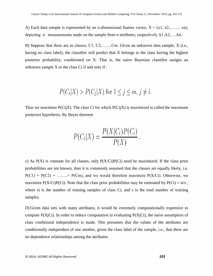
A) Each data sample is represented by an n-dimensional feature vector, X = (x1, x2,…….. xn),

depicting n measurements made on the sample from n attributes, respectively A1,A2,….An.

B) Suppose that there are m classes, C1, C2, ……Cm. Given an unknown data sample, X (i.e.,

having no class label), the classifier will predict that X belongs to the class having the highest

posterior probability, conditioned on X. That is, the naive Bayesian classifier assigns an

unknown sample X to the class Ci if and only if :

Thus we maximize P(CijX). The class Ci for which P(CijX) is maximized is called the maximum

posteriori hypothesis. By Bayes theorem

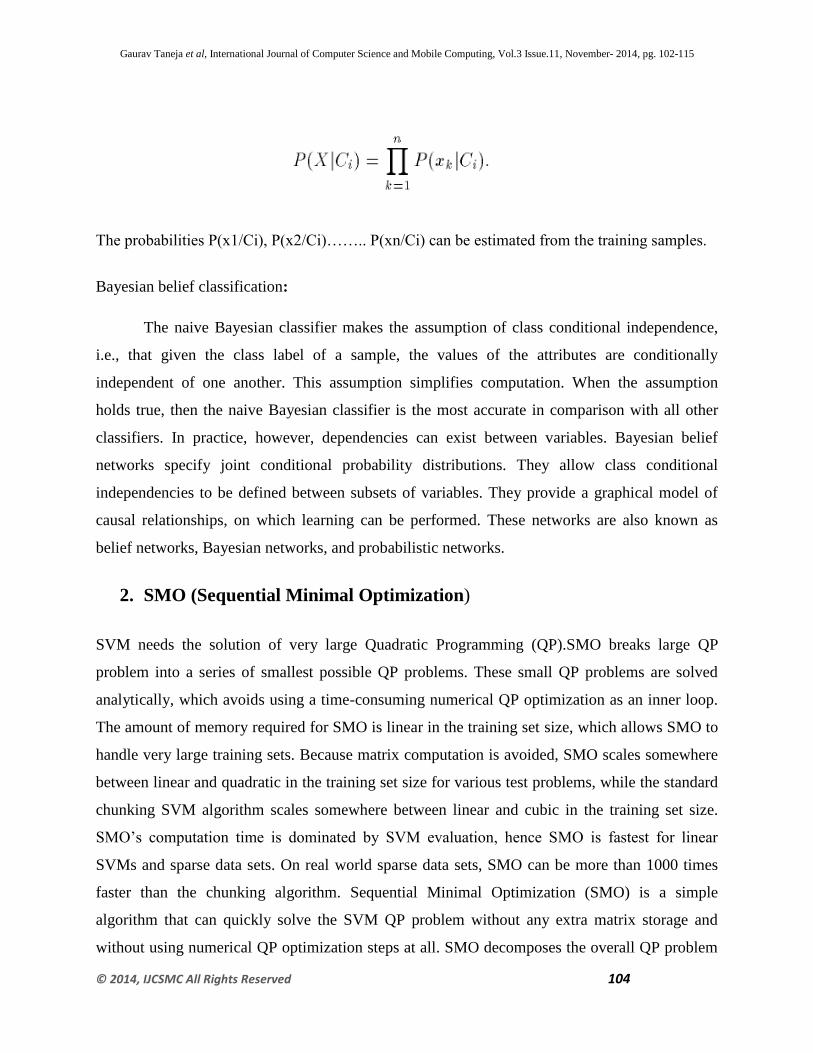
c) As P(X) is constant for all classes, only P(X/Ci)P(Ci) need be maximized. If the class prior

probabilities are not known, then it is commonly assumed that the classes are equally likely, i.e.

P(C1) = P(C2) = ……..= P(Cm), and we would therefore maximize P(X/Ci). Otherwise, we

maximize P(X/Ci)P(Ci). Note that the class prior probabilities may be estimated by P(Ci) = si/s ,

where si is the number of training samples of class Ci, and s is the total number of training

samples.

D) Given data sets with many attributes, it would be extremely computationally expensive to

compute P(XjCi). In order to reduce computation in evaluating P(XjCi), the naive assumption of

class conditional independence is made. This presumes that the values of the attributes are

conditionally independent of one another, given the class label of the sample, i.e., that there are

no dependence relationships among the attributes.



The probabilities P(x1/Ci), P(x2/Ci)…….. P(xn/Ci) can be estimated from the training samples.

Bayesian belief classification:

The naive Bayesian classifier makes the assumption of class conditional independence,

i.e., that given the class label of a sample, the values of the attributes are conditionally

independent of one another. This assumption simplifies computation. When the assumption

holds true, then the naive Bayesian classifier is the most accurate in comparison with all other

classifiers. In practice, however, dependencies can exist between variables. Bayesian belief

networks specify joint conditional probability distributions. They allow class conditional

independencies to be defined between subsets of variables. They provide a graphical model of

causal relationships, on which learning can be performed. These networks are also known as

belief networks, Bayesian networks, and probabilistic networks.

2. SMO (Sequential Minimal Optimization)

SVM needs the solution of very large Quadratic Programming (QP).SMO breaks large QP

problem into a series of smallest possible QP problems. These small QP problems are solved

analytically, which avoids using a time-consuming numerical QP optimization as an inner loop.

The amount of memory required for SMO is linear in the training set size, which allows SMO to

handle very large training sets. Because matrix computation is avoided, SMO scales somewhere

between linear and quadratic in the training set size for various test problems, while the standard

chunking SVM algorithm scales somewhere between linear and cubic in the training set size.

SMO’s computation time is dominated by SVM evaluation, hence SMO is fastest for linear

SVMs and sparse data sets. On real world sparse data sets, SMO can be more than 1000 times

faster than the chunking algorithm. Sequential Minimal Optimization (SMO) is a simple

algorithm that can quickly solve the SVM QP problem without any extra matrix storage and

without using numerical QP optimization steps at all. SMO decomposes the overall QP problem



into QP sub-problems, using Osuna’s theorem to ensure convergence. Unlike the previous

methods, SMO chooses to solve the smallest possible optimization problem at every step. For the

standard SVM QP problem, the smallest possible optimization problem involves two Lagrange

multipliers, because the Lagrange multipliers must obey a linear equality constraint. At every

step, SMO chooses two Lagrange multipliers to jointly optimize, finds the optimal values for

these multipliers, and updates the SVM to reflect the new optimal values. The advantage of SMO

lies in the fact that solving for two Lagrange multipliers can be done analytically. Thus,

numerical QP optimization is avoided entirely. The inner loop of the algorithm can be expressed

in a short amount of C code, rather than invoking an entire QP library routine. Even though more

optimization sub-problems are solved in the course of the algorithm, each sub-problem is so fast

that the overall QP problem is solved quickly.

In addition, SMO requires no extra matrix storage at all. Thus, very large SVM training

problems can fit inside of the memory of an ordinary personal computer or workstation. Because

no matrix algorithms are used in SMO, it is less susceptible to numerical precision problems.

There are two components to SMO: an analytic method for solving for the two Lagrange

multipliers, and a heuristic for choosing which multipliers to optimize.

3. NBTree (The Hybrid Algorithm)

The NBTree algorithm is similar to the classical recursive partitioning schemes except that the

leaf nodes created are Naïve Bayes categorizers instead of nodes predicting a single class.

A threshold for continuous attributes is chosen using the standard entropy minimization

technique as is done for decision trees_ The utility of a node is computed by discretizing the data

and computing fold cross validation accuracy estimate of using Naïve Bayes at the node_ The

utility of a split is the weighted sum of the utility of the nodes where the weight given to a node

is proportional to the number of instances that go down to that node.



TERMINOLOGY

Imagine a study evaluating a new test that screens people for a disease. Each person taking

the test either has or does not have the disease. The test outcome can be positive (predicting that

the person has the disease) or negative (predicting that the person does not have the disease). The

test results for each subject may or may not match the subject's actual status. In that setting:

True positive: Sick people correctly diagnosed as sick

False positive: Healthy people incorrectly identified as sick

True negative: Healthy people correctly identified as healthy

False negative: Sick people incorrectly identified as healthy

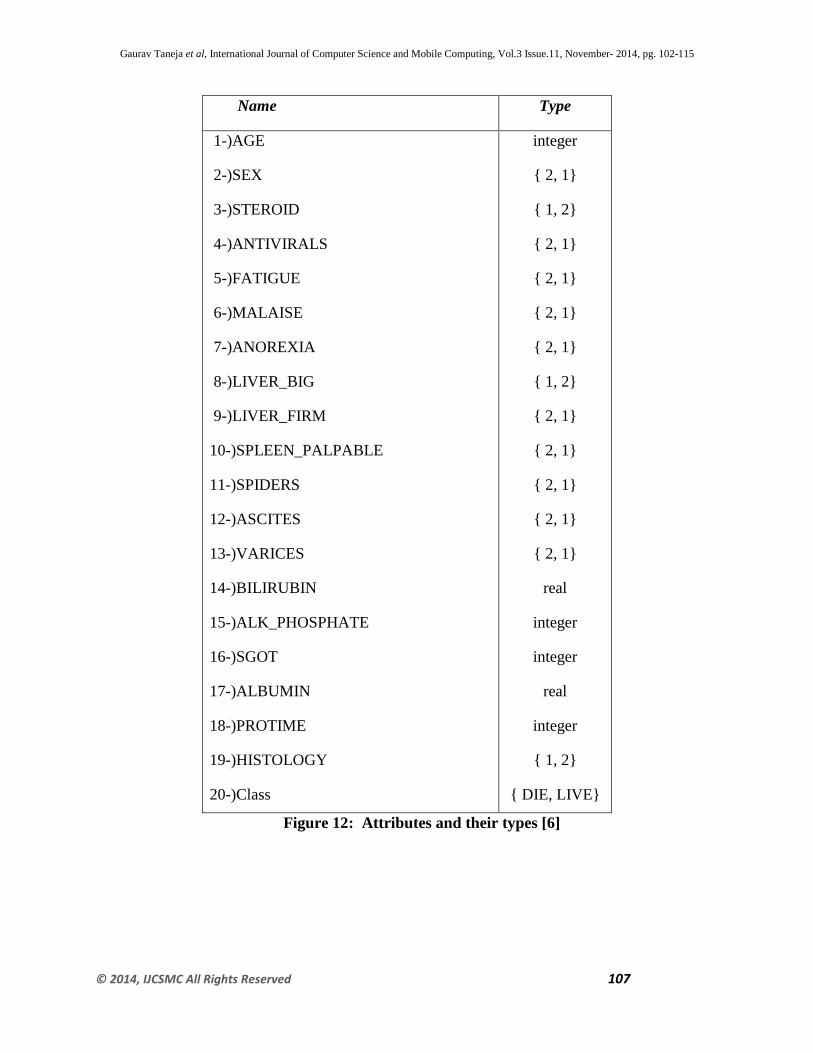
HEPATITIS DATASET

It contains 153 instances and 20 attributes, in which 9 instances are having missing values. It is a

health care dataset. It has been taken from UCI Machine Repository(source). The fields

(attributes) name are…..

AGE

SEX

STEROID

MALAISE

PROTIME

HISTOLOG

CLASS (LIVE/DEAD) etc.

And instances are like-(42,female,yes,no,yes,no,no,yes,yes,………..0.9,0.2,80,dead)



Name Type

1-)AGE

2-)SEX

3-)STEROID

4-)ANTIVIRALS

5-)FATIGUE

6-)MALAISE

7-)ANOREXIA

8-)LIVER_BIG

9-)LIVER_FIRM

10-)SPLEEN_PALPABLE

11-)SPIDERS

12-)ASCITES

13-)VARICES

14-)BILIRUBIN

15-)ALK_PHOSPHATE

16-)SGOT

17-)ALBUMIN

18-)PROTIME

19-)HISTOLOGY

20-)Class

integer

{ 2, 1}

{ 1, 2}

{ 2, 1}

{ 2, 1}

{ 2, 1}

{ 2, 1}

{ 1, 2}

{ 2, 1}

{ 2, 1}

{ 2, 1}

{ 2, 1}

{ 2, 1}

real

integer

integer

real

integer

{ 1, 2}

{ DIE, LIVE}

Figure 12: Attributes and their types [6]



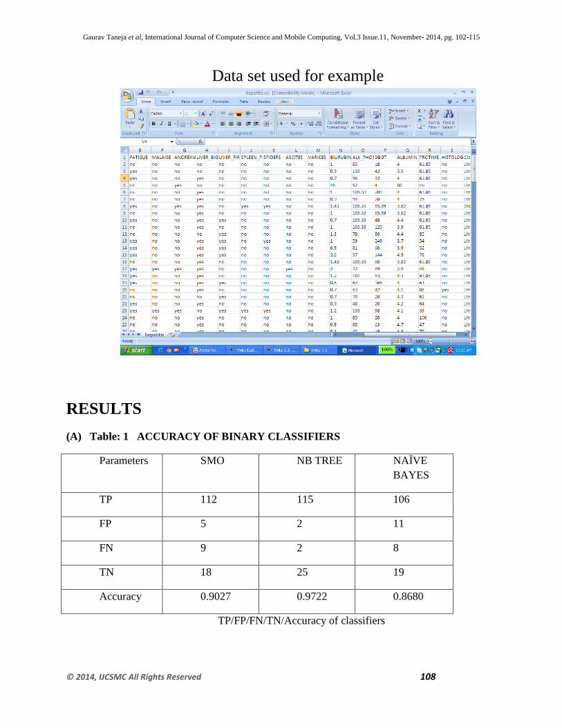
Data set used for example

RESULTS

(A) Table: 1 ACCURACY OF BINARY CLASSIFIERS

Parameters SMO NB TREE NAÏVE

BAYES

TP 112 115 106

FP 5 2 11

FN 9 2 8

TN 18 25 19

Accuracy 0.9027 0.9722 0.8680

TP/FP/FN/TN/Accuracy of classifiers



FIGURE 1: TP/FP/FN/TN/Accuracy of Classifiers

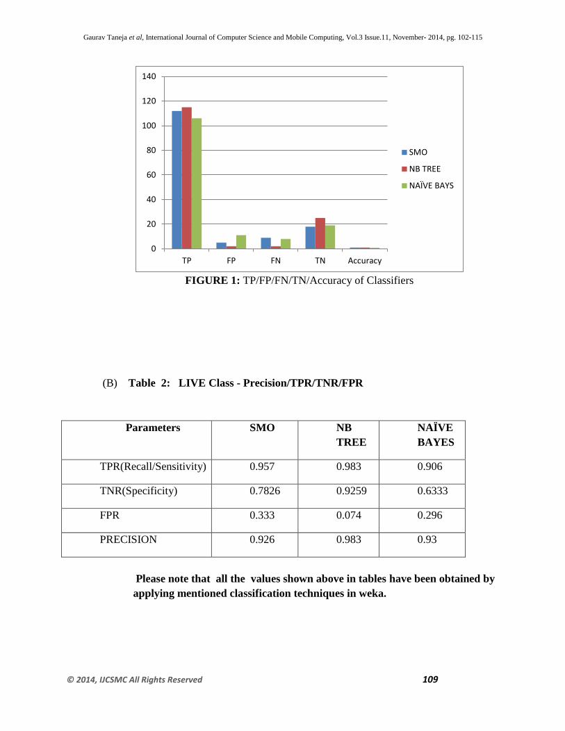
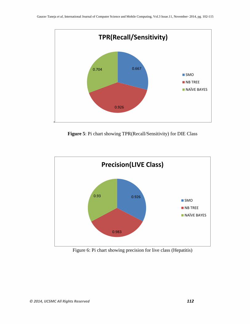
(B) Table 2: LIVE Class - Precision/TPR/TNR/FPR

Parameters SMO NB

TREE

NAÏVE

BAYES

TPR(Recall/Sensitivity) 0.957 0.983 0.906

TNR(Specificity) 0.7826 0.9259 0.6333

FPR 0.333 0.074 0.296

PRECISION 0.926 0.983 0.93

Please note that all the values shown above in tables have been obtained by

applying mentioned classification techniques in weka.

0

20

40

60

80

100

120

140

TP FP FN TN Accuracy

SMO

NB TREE

NAÏVE BAYS



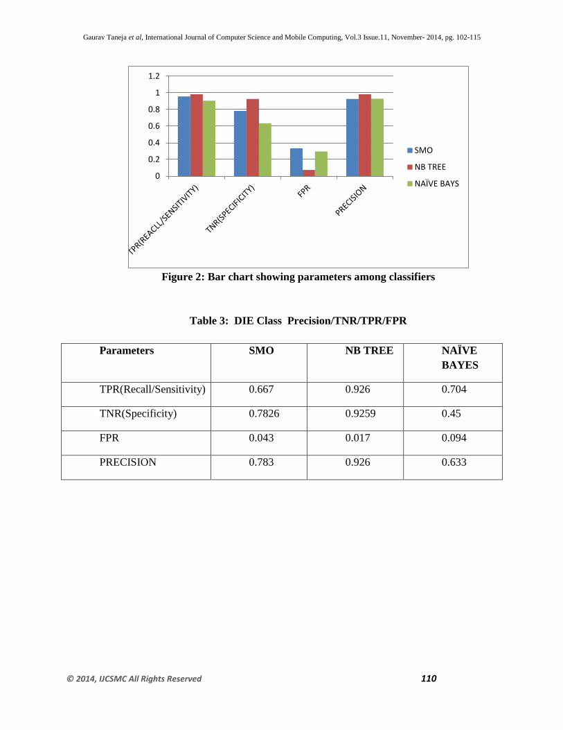
Figure 2: Bar chart showing parameters among classifiers

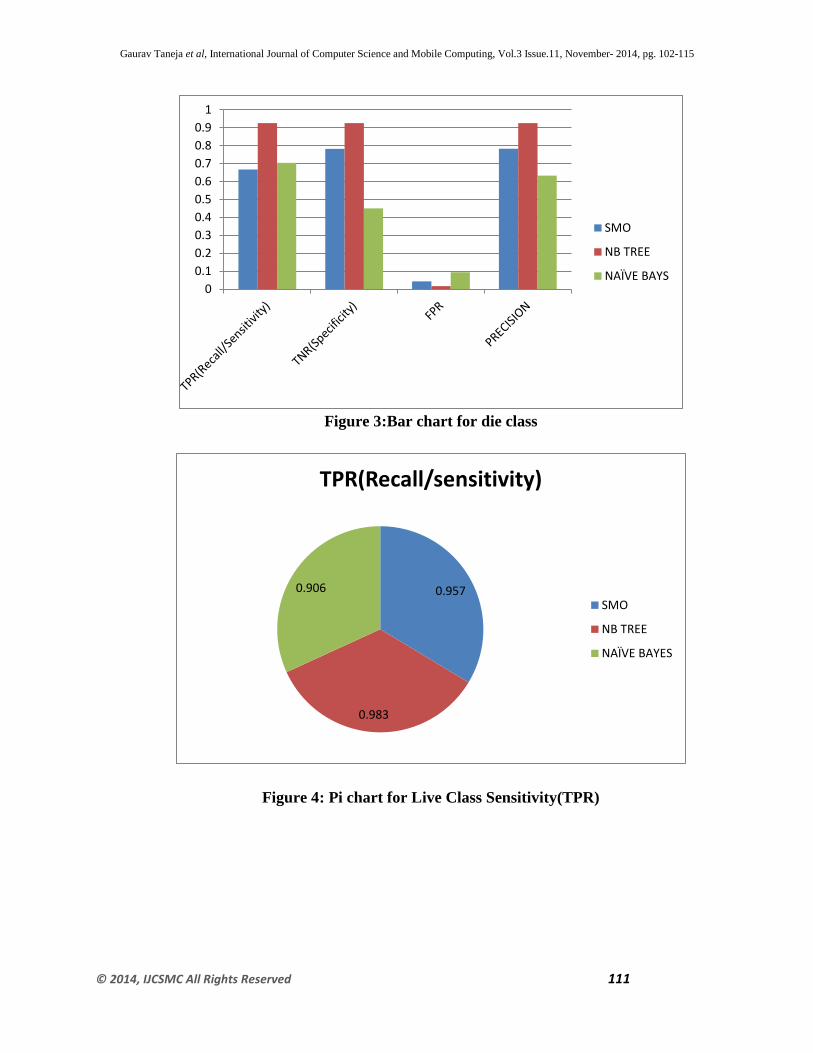
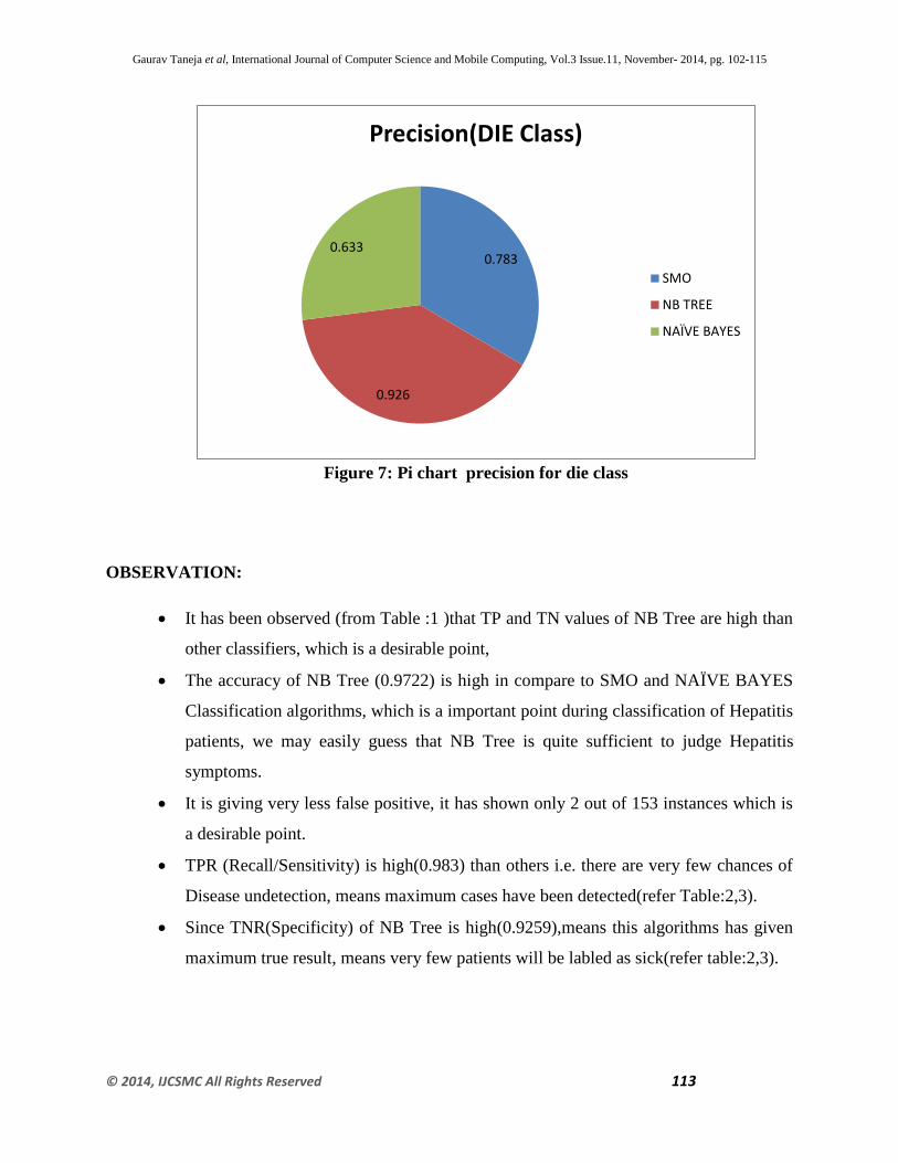
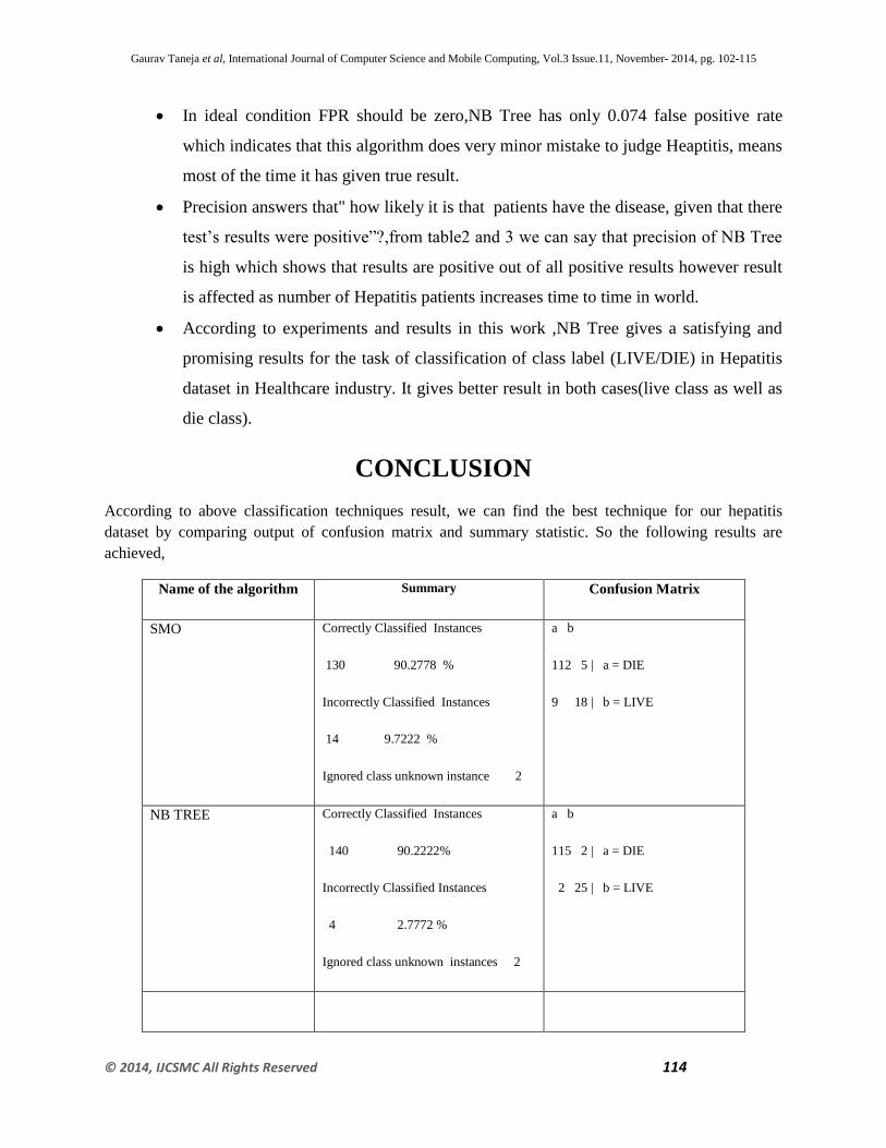
Table 3: DIE Class Precision/TNR/TPR/FPR

Parameters SMO NB TREE NAÏVE

BAYES

TPR(Recall/Sensitivity) 0.667 0.926 0.704

TNR(Specificity) 0.7826 0.9259 0.45

FPR 0.043 0.017 0.094

PRECISION 0.783 0.926 0.633

0

0.2

0.4

0.6

0.8

1

1.2

SMO

NB TREE

NAÏVE BAYS



Figure 3:Bar chart for die class

Figure 4: Pi chart for Live Class Sensitivity(TPR)

0

0.1

0.2

0.3

0.4

0.5

0.6

0.7

0.8

0.9

1

SMO

NB TREE

NAÏVE BAYS

0.957

0.983

0.906

TPR(Recall/sensitivity)

SMO

NB TREE

NAÏVE BAYES



.

Figure 5: Pi chart showing TPR(Recall/Sensitivity) for DIE Class

Figure 6: Pi chart showing precision for live class (Hepatitis)

0.667

0.926

0.704

TPR(Recall/Sensitivity)

SMO

NB TREE

NAÏVE BAYES

0.926

0.983

0.93

Precision(LIVE Class)

SMO

NB TREE

NAÏVE BAYES



Figure 7: Pi chart precision for die class

OBSERVATION:

It has been observed (from Table :1 )that TP and TN values of NB Tree are high than

other classifiers, which is a desirable point,

The accuracy of NB Tree (0.9722) is high in compare to SMO and NAÏVE BAYES

Classification algorithms, which is a important point during classification of Hepatitis

patients, we may easily guess that NB Tree is quite sufficient to judge Hepatitis

symptoms.

It is giving very less false positive, it has shown only 2 out of 153 instances which is

a desirable point.

TPR (Recall/Sensitivity) is high(0.983) than others i.e. there are very few chances of

Disease undetection, means maximum cases have been detected(refer Table:2,3).

Since TNR(Specificity) of NB Tree is high(0.9259),means this algorithms has given

maximum true result, means very few patients will be labled as sick(refer table:2,3).

0.783

0.926

0.633

Precision(DIE Class)

SMO

NB TREE

NAÏVE BAYES



In ideal condition FPR should be zero,NB Tree has only 0.074 false positive rate

which indicates that this algorithm does very minor mistake to judge Heaptitis, means

most of the time it has given true result.

Precision answers that" how likely it is that patients have the disease, given that there

test’s results were positive”?,from table2 and 3 we can say that precision of NB Tree

is high which shows that results are positive out of all positive results however result

is affected as number of Hepatitis patients increases time to time in world.

According to experiments and results in this work ,NB Tree gives a satisfying and

promising results for the task of classification of class label (LIVE/DIE) in Hepatitis

dataset in Healthcare industry. It gives better result in both cases(live class as well as

die class).

CONCLUSION

According to above classification techniques result, we can find the best technique for our hepatitis

dataset by comparing output of confusion matrix and summary statistic. So the following results are

achieved,

Name of the algorithm Summary Confusion Matrix

SMO Correctly Classified Instances

130 90.2778 %

Incorrectly Classified Instances

14 9.7222 %

Ignored class unknown instance 2

a b

112 5 | a = DIE

9 18 | b = LIVE

NB TREE Correctly Classified Instances

140 90.2222%


4 2.7772 %

Ignored class unknown instances 2

a b

115 2 | a = DIE

2 25 | b = LIVE



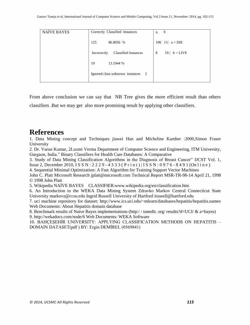
NAÏVE BAYES Correctly Classified Instances

125 86.8056 %


19 13.1944 %

Ignored class unknown instances 2

a, b

106 11| a = DIE

8 19 | b = LIVE

From above conclusion we can say that NB Tree gives the more efficient result than others

classifiers .But we may get also more promising result by applying other classifiers.

References

1. Data Mining concept and Techniques jiawei Han and Micheline Kamber :2000,Simon Fraser

University

2. Dr. Varun Kumar, 2Luxmi Verma Department of Computer Science and Engineering, ITM University,

Gurgaon, India.” Binary Classifiers for Health Care Databases: A Comparative

3. Study of Data Mining Classification Algorithms in the Diagnosis of Breast Cancer” IJCST Vol. 1,

Issue 2, December 2010, I S S N : 2 2 2 9 - 4 3 3 3 ( P r i n t ) | I S S N : 0 9 7 6 - 8 4 9 1 (On l i n e )

4. Sequential Minimal Optimization: A Fast Algorithm for Training Support Vector Machines

John C. Platt Microsoft Research [email protected] Technical Report MSR-TR-98-14 April 21, 1998

© 1998 John Platt

5. Wikipedia NAÏVE BAYES CLASSIFIER:www.wikipedia.org/en/classification.htm

6. An Introduction to the WEKA Data Mining System Zdravko Markov Central Connecticut State

University [email protected] Ingrid Russell University of Hartford [email protected]

7. uci machine repository for dataset: http://www.ics.uci.edu/~mlearn/databases/hepatitis/hepatitis.names

Web Documents: About Hepatitis domain database

8. Benchmark results of Naive Bayes implementations (http:/ / tunedit. org/ results?d=UCI/ & a=bayes)

9. http://wekadocs.com/node/6 Web Documents: WEKA Software

10. BAHÇEŞEHİR UNIVERSITY: APPLYING CLASSIFICATION METHODS ON HEPATITIS –

DOMAIN DATASET(pdf ) BY: Ergin DEMİREL (0569841)

mailto:[email protected]



http://www.ics.uci.edu/~mlearn/databases/hepatitis/hepatitis.names

http://wekadocs.com/node/6