Fast and Reliable Reconstruction of Phylogenetic Trees withVery Short Edges∗

(Draft)

Ilan Gronau† Shlomo Moran‡ Sagi Snir§

January 17, 2008

Abstract

Phylogenetic reconstruction methods deal with the problem of reconstructing a treedescribing the evolution of a given set of species; this is usually done using sequencesof characters (e.g. DNA) extracted from these species. A central goal in the designof these methods is to be able to guarantee accurate reconstruction (with high prob-ability) from short input sequences. Under common models of evolution, the requiredsequence length is known to depend on the depth of the tree as well as on its minimaledge-weight. Fast converging reconstruction algorithms are considered state-of the-artin this context, as they require asymptotically minimal sequence length in order to ac-curately reconstruct the entire tree. However, when the tree in question contains veryshort edges, the sequence length required for complete (and accurate) topological res-olution may be too long for practical purposes. This calls for adaptive fast convergingalgorithms studied in this paper, which, given input sequences of any length, correctlyreconstruct as many edges of the evolutionary tree as possible.

In this paper we present a fast converging reconstruction algorithm which returnsa partially resolved topology containing no false edges and all “sufficiently long” edgesof the underlying phylogenetic tree. The weight of edges our algorithm guarantees toreconstruct is determined by the input sequence length and the depth of the tree; itdoes not depend, however, on the minimal edge-weight of the tree, and in this aspectit is strictly stronger than any previously known edge-reconstruction guarantee. Thisfact, together with the optimal complexity of our algorithm (linear space and quadratic-time), makes it appealing for practical use.

1 Introduction.

Phylogenetic reconstruction is the task of figuring out the evolutionary history of a givenset of extant species (taxa). This history is usually described by an edge-weighted treewhose internal vertices represent past speciation events (extinct species) and whose leavescorrespond to the given set of taxa. The (positive) weight of an edge in this tree describesthe amount of evolutionary change between the two speciation events it connects. Recon-struction methods typically receive as input an alignment of sequences, each correspondingto a different taxon, and they are expected to yield a tree which closely depicts the truephylogenetic tree. In this work we only consider the topology of the output tree, which is es-sentially its unrooted and unweighted description (disregarding all zero-weight edges). Theoutput topology is said to be fully resolved if the degree of each internal vertex is exactlythree. We compare the output topology with the original phylogenetic tree by comparing

∗A preliminary version of this paper appeared in the proceedings of SODA08†Technion - Israel Institute of Technology, Haifa, 32000Israel‡Technion - Israel Institute of Technology, Haifa, 32000Israel§Netanya Academic College, Netanya, Israel

1

the splits induced by their edges on the set of taxa. In other words, an edge of the originaltree is said to be correctly reconstructed if the output tree contains an edge inducing thesame split.

A major challenge in designing reconstruction algorithms is being able to guaranteea maximum amount of correct reconstruction from short alignments. Studies providingsuch reconstruction guarantees usually assumes some (relatively simple) model of sequenceevolution, such as the Cavender-Farris-Neyman (CFN) model for binary sequences [5, 15, 25],or the Jukes-Cantor model for DNA sequences [19]. Many results in this field focus ondetermining the minimal sequence length required for correct reconstruction of the entirephylogenetic tree. These results show that this sequence-length depends on the weight ofthe shortest edge in the tree and on some notion of tree-depth. It was already shown in [13]that correct reconstruction can be guaranteed (w.h.p.) from sequences of length:

k = O

(log(n)

f2· exp(depth)

), (1)

where n is the number of taxa, f is the minimal edge weight in the tree, and depth isthe depth of the tree (see Definition 6.5). In [22, 24] it is shown that this is the optimaldependence (up to constants) in f and depth for general trees, and in [12] it is shown that the(exponential) dependence on depth can be eliminated from §1, when assuming an additionalspecific upper bound on edge weights. So for general trees, the algorithm suggested in [13]requires asymptotically optimal sequence length. Note that if g is an upper bound on edgeweight in T , then depth ≤ g log2(n), and §1 reduces to the following polynomial dependencein n:

k =nO(g)

f2. (2)

Much attention has been focused in recent years on designing other algorithms whichprovide a similar guarantee to that of [13] (see e.g. [14, 18, 7, 8, 20, 22, 23, 11]). Suchreconstruction methods are often said to be fast converging (they are called absolutely fastconverging if they do not require a prior knowledge of the lower and upper bounds on edgelengths [21]). Whereas fast converging algorithms minimize the sequence length requiredfor correct reconstruction of any given tree, most of them do not attempt to maximize theamount of correct reconstruction when the input sequences are too short to ensure correctreconstruction of the entire tree. In fact, the great majority of fast converging algorithms failto produce any meaningful output in such a case. This poses an obvious problem when tryingto apply such algorithms on actual (and even simulated) data. The forest reconstructionalgorithms of [23, 11] are the only fast converging algorithms known today which attemptto cope with this problem. When the sequences are too short for complete reconstruction,these algorithms return a forest of fully resolved edge-disjoint trees which are consistent(w.h.p) with the original tree. Whereas this approach allows correct reconstruction of the‘shallow’ edges in the tree, the presence of some short edges may prevent such algorithmsfrom reconstructing long edges situated deeper in the tree, as demonstrated by the followingexample.

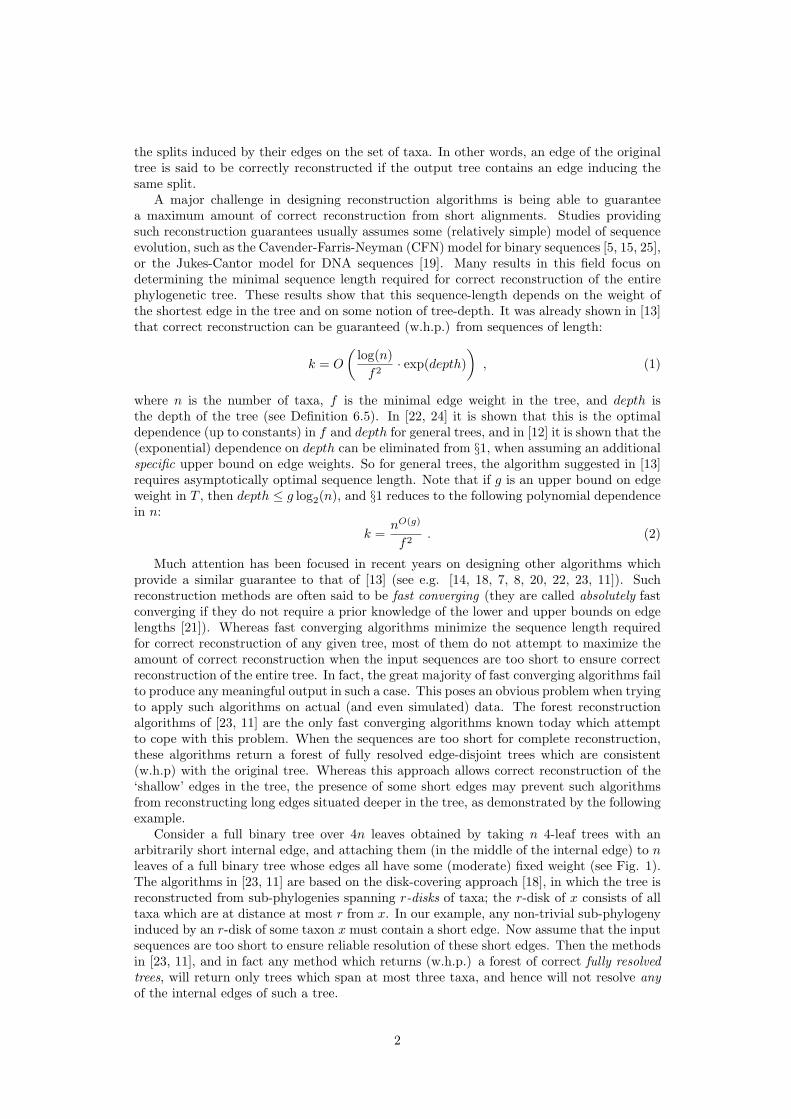
Consider a full binary tree over 4n leaves obtained by taking n 4-leaf trees with anarbitrarily short internal edge, and attaching them (in the middle of the internal edge) to nleaves of a full binary tree whose edges all have some (moderate) fixed weight (see Fig. 1).The algorithms in [23, 11] are based on the disk-covering approach [18], in which the tree isreconstructed from sub-phylogenies spanning r-disks of taxa; the r-disk of x consists of alltaxa which are at distance at most r from x. In our example, any non-trivial sub-phylogenyinduced by an r-disk of some taxon x must contain a short edge. Now assume that the inputsequences are too short to ensure reliable resolution of these short edges. Then the methodsin [23, 11], and in fact any method which returns (w.h.p.) a forest of correct fully resolvedtrees, will return only trees which span at most three taxa, and hence will not resolve anyof the internal edges of such a tree.

2

1 2 3 4 … 4n

Figure 1: Forest Reconstruction. Consider the above full binary tree and assume thatthe edges in the highlighted layer are too short to be reconstructed by the input sequences.Then any disk-covering method which returns a forest of fully resolved trees will not be ableto reconstruct any of the internal edges (even the longer ones).

The above example demonstrates the sensitivity of fast converging algorithms to the ex-istence of short edges in the tree. This motivates the following extension of fast convergence:

Definition 1.1. A reconstruction algorithm is said to be adaptive fast converging if itaccurately reconstruct all edges of weight greater than ε (w.h.p.), from sequences of length

k =nO(g)

ε2. (3)

In this paper we present a technique which enables reconstruction of adaptive fast con-verging algorithms by contracting low-confidence edges (and thus introducing high degreevertices). This technique guarantees that: (1) the returned topology contains no false pos-itives (i.e. edges inducing incorrect splits), and (2) the missing edges correspond only to“short” edges of the original tree. After introducing the general technique, we show how itcan be applied on pairwise dissimilarity data (extracted from the input sequences) to obtainan adaptive fast converging algorithm. Contraction of low-confidence edges is an approachwhich exists in other known reconstruction methods, such as Buneman’s classic algorithmand its refinements (see eg [4, 2]). However, our technique results in a more efficient algo-rithm, and it is adaptive fast converging, and thus allows the reconstruction of much shorteredges than ones reconstructed by Buneman’s algorithm.

The algorithm presented in this paper follows the incremental approach which was intro-duced in [3], and later applied to fast converging algorithms in [9, 8, 20]. In this approach,the topology is constructed by attaching the taxa one by one. The goal in each iteration is tofind the correct place of insertion of the new taxon in the current topology. This is typicallydone by querying the vertices of the current topology as to the direction (relative to thatspecific vertex) in which the new taxon should be attached. When a vertex in the currenttopology corresponds to a vertex of the original tree, such directional queries can be simplyanswered by querying quartet splits (see [9, 8]). Our directional queries may fail to returna direction when it is not confident enough in the answer. In such a case, the introductionof false edges is avoided by contracting some of the previously constructed edges. As aresult, the topology maintained by our incremental algorithm may contain vertices whichcorrespond to (contracted) subtrees of the original tree. This significantly complicates thetask of reliably answering a directional query, but we manage to accomplish this task withinthe asymptotic optimal time complexity of O(n2).The performance of our basic algorithm depends on a bound on the diameter of the con-tracted subtrees, which in extreme cases can be very large. In the final section of thispaper we present a method which avoids this dependence, and thus imply the adaptive fastconvergence of the algorithm.

3

In the next section we present the notations used in the paper. In Sections 3-6 wepresent our basic incremental algorithm in a ‘top-down’ fashion: In Section 3 we outline ouralgorithm and present the concept of partial directional oracle which is a model-independentprimitive for constructing phylogenetic trees in the presence of noisy information. In Section4 we prove some basic properties of our algorithm. In Section 5 we present an implementationof a directional oracle which uses a reliable quartet oracle. In Section 6 we present andanalyze an implementation of our algorithm from a noisy version of the additive metricinduced by the original tree. In Section 7 we analyze the time and space complexities ofour algorithm, and in Section 8 we discuss the performance of our algorithm on a commonmodel of sequence evolution. In the final section of this paper we present a modification ofthe basic algorithm (as presented in sections 3-6), which achieves adaptive fast convergence.

2 Definitions and Notations.

Trees: A tree T is an undirected connected and acyclic graph. V (T ) and E(T ) denotethe sets of vertices and edges of T , respectively. leaves(T ) denotes the leaf-set of T ,and internal(T ) = V (T ) \ leaves(T ) denotes the set of its internal vertices. For a ver-tex v ∈ V (T ), the neighborhood of v, NT (v), is the set of vertices adjacent to v in T .The neighborhood of a subset U ⊆ V is defined by NT (U) = ∪u∈UN(u) \ U . The degreeof a vertex, degT (v), is the size of its neighborhood in T . The parent of a leaf x in T ,parentT (x), is the unique vertex in NT (x). T is said to be a phylogenetic tree over taxon-setS if leaves(T ) = S, the degree of every internal vertex is at least three, and every edgee ∈ E(T ) is associated with a strictly positive weight w(e). The weight function w inducesa metric DT = {dT (u, v)}u,v∈V (T ) over V (T ), s.t. dT (u, v) is the total weight of pathT (u, v)– the (unique) simple path connecting u and v in T . The diameter of T (diam(T )) is themaximum weight of a simple path in T .

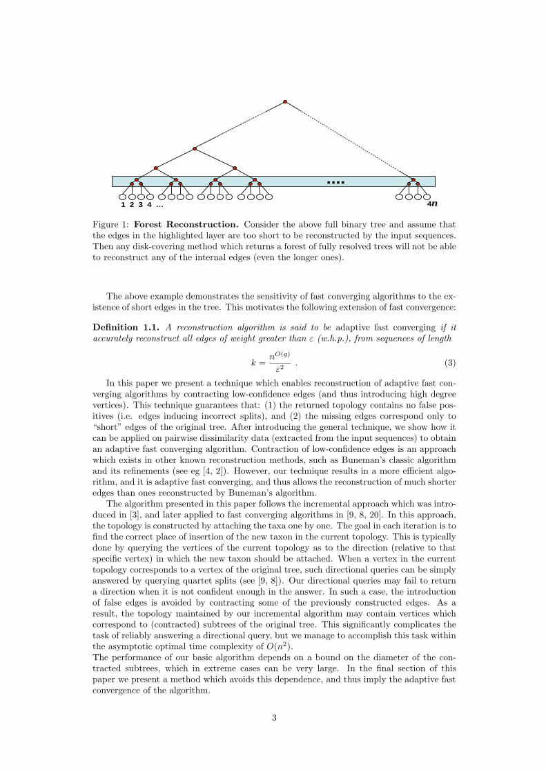
A subtree of a tree T is a connected subgraph of T . The notion of distances is generalizedfor subtrees as follows: for two vertex disjoint subtrees t1, t2 of T , dT (t1, t2) denotes the totalweight of pathT (t1, t2), which is the (unique) shortest path in T connecting a vertex in t1and a vertex in t2. Let t1, t2, t3 be mutually disjoint subtrees of T . We say that t2 separatest1 from t3 if pathT (t1, t3) intersects t2. If t2 does not separate t1 from t3 we say that t1and t3 are on the same side of t2 (see Fig. 2). In general, we use lower case t’s to denotesubtrees of a tree T , and whenever the tree T is clear from context, the subscript T may beremoved from the corresponding notation.

u

v

w

x

Figure 2: In the above tree, x separates u from v and from w. v, x and w are all on thesame side of u.

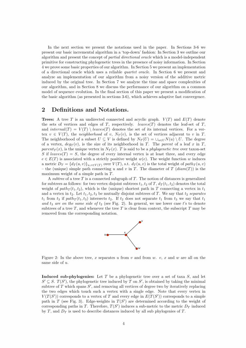
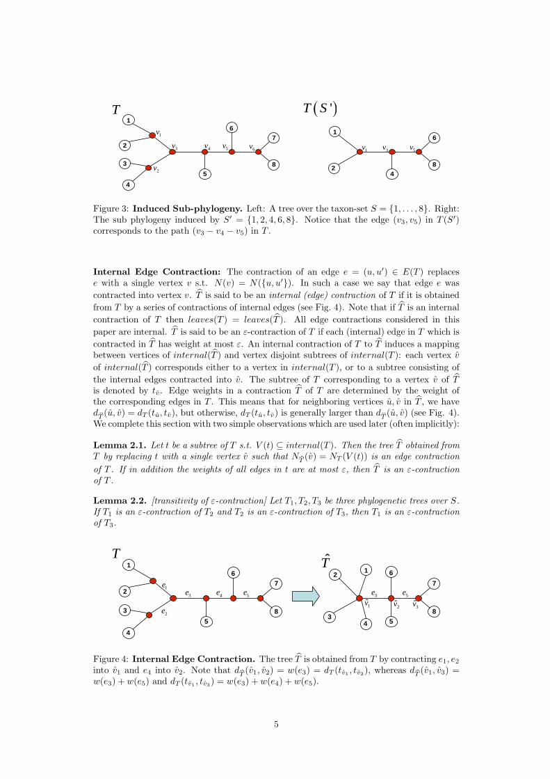
Induced sub-phylogenies: Let T be a phylogenetic tree over a set of taxa S, and letS′ ⊆ S. T (S′), the phylogenetic tree induced by T on S′, is obtained by taking the minimalsubtree of T which spans S′, and removing all vertices of degree two by iteratively replacingthe two edges which touch such a vertex with a single edge. Note that every vertex inV (T (S′)) corresponds to a vertex of T and every edge in E(T (S′)) corresponds to a simplepath in T (see Fig. 3). Edge-weights in T (S′) are determined according to the weight ofcorresponding paths in T . Therefore, T (S′) induces a sub-metric to the metric DT inducedby T , and DT is used to describe distances induced by all sub phylogenies of T .

4

6

5

1

2

3

4

7

8

1v

T

4

1

2

6

8

( )'T S

2v

3v 4v 5v6v

1v 3v 5v

Figure 3: Induced Sub-phylogeny. Left: A tree over the taxon-set S = {1, . . . , 8}. Right:The sub phylogeny induced by S′ = {1, 2, 4, 6, 8}. Notice that the edge (v3, v5) in T (S′)corresponds to the path (v3 − v4 − v5) in T .

Internal Edge Contraction: The contraction of an edge e = (u, u′) ∈ E(T ) replacese with a single vertex v s.t. N(v) = N({u, u′}). In such a case we say that edge e wascontracted into vertex v. T is said to be an internal (edge) contraction of T if it is obtainedfrom T by a series of contractions of internal edges (see Fig. 4). Note that if T is an internalcontraction of T then leaves(T ) = leaves(T ). All edge contractions considered in thispaper are internal. T is said to be an ε-contraction of T if each (internal) edge in T which iscontracted in T has weight at most ε. An internal contraction of T to T induces a mappingbetween vertices of internal(T ) and vertex disjoint subtrees of internal(T ): each vertex v

of internal(T ) corresponds either to a vertex in internal(T ), or to a subtree consisting ofthe internal edges contracted into v. The subtree of T corresponding to a vertex v of Tis denoted by tv. Edge weights in a contraction T of T are determined by the weight ofthe corresponding edges in T . This means that for neighboring vertices u, v in T , we havedbT (u, v) = dT (tu, tv), but otherwise, dT (tu, tv) is generally larger than dbT (u, v) (see Fig. 4).We complete this section with two simple observations which are used later (often implicitly):

Lemma 2.1. Let t be a subtree of T s.t. V (t) ⊆ internal(T ). Then the tree T obtained fromT by replacing t with a single vertex v such that NbT (v) = NT (V (t)) is an edge contractionof T . If in addition the weights of all edges in t are at most ε, then T is an ε-contractionof T .

Lemma 2.2. [transitivity of ε-contraction] Let T1, T2, T3 be three phylogenetic trees over S.If T1 is an ε-contraction of T2 and T2 is an ε-contraction of T3, then T1 is an ε-contractionof T3.

1v2v 3v

6

5

1

2

3

4

7

8

1e

6

5

12

34

7

8

TT

2e

3e 4e 5e 3e 5e

Figure 4: Internal Edge Contraction. The tree T is obtained from T by contracting e1, e2

into v1 and e4 into v2. Note that dbT (v1, v2) = w(e3) = dT (tv1 , tv2), whereas dbT (v1, v3) =w(e3) + w(e5) and dT (tv1 , tv3) = w(e3) + w(e4) + w(e5).

5

3 Basics of the Incremental Algorithm.

Our incremental reconstruction algorithm works in iterations, where the objective in eachiteration is to extend an edge contraction of T (S′) for some S′ ⊆ S to an edge-contractionof T (S′ ∪ {x}) for some x ∈ S \ S′.

Procedure Incremental Reconstruct(S):– Select x0, x1 ∈ S, and initialize: T ← (x0, x1) ; S′ ← {x0, x1}.– While S′ 6= S do:

1. Select a taxon x ∈ S \ S′ and set S′ ← S′ ∪ {x}.2. Attach Taxon(T , x)

The crucial part of this process is pinpointing the anchor of x, which is the location ofparent(x) in the current topology, as defined below.

Definition 3.1 (Anchor). Let T be an edge contraction of T (S′), and let x ∈ S \ S′. Theanchor of x in T , anchorbT (x), is defined as follows: Let px be the parent of x in T (S′∪{x}).If px is included in tv for some v ∈ V (T ) (either by being a vertex in tv or by lying on a pathin T which corresponds to an edge of tv), then anchorbT (x) = v. Otherwise, anchorbT (x) isthe unique edge (u, v) ∈ E(T ) for which px is an internal vertex in pathT (tu, tv).

The anchor of x in T is found by querying vertices in T for the location of x. Thesequeries are posed to a directional oracle which receives the new taxon x and a vertex v of Tand is expected to output the neighbor u of v which indicates the direction of x with respectto v (if such a neighbor exists).

Definition 3.2 (Partial Directional Oracle). Let T be a phylogenetic tree over S. A partialdirectional oracle for T is a function PDO = PDOT which receives queries of the form(T , v, x), where

• T is an edge-contraction of T (S′), for some S′ ⊂ S,

• v ∈ V (T ),

• x ∈ S \ S′,

and outputs either a vertex u ∈ NbT (v) or ‘null’. The output must satisfy two requirements:

• If v ∈ leaves(T ), then PDO(T , v, x) = parentbT (v).

• If PDO(T , v, x) = u, then tu and x are on the same side of tv in T (S′ ∪ {x}) (thisproperty is also referred to as the truthfulness of the oracle). We sometimes abusenotation and simply say that u is on the same side of v as x.

Our algorithm uses the partial directional oracle to compute the insertion zone of x in T .

Definition 3.3 (Insertion Zone). Given an edge-contraction T of T (S′), some taxon x ∈S \ S′, and a partial directional oracle PDO, the insertion zone of x in T , denoted bytinz(T , x, PDO) (or simply tinz when T , x and PDO are clear from context), is the subtreeof T defined by the following procedure:

Procedure Find Insertion Zone(T , x, PDO):

1. tinz ← T

2. For every edge (u, v) ∈ E(tinz) s.t. PDO(T , v, x) = u do:– Delete from tinz all the vertices which are separated from u by v.

6

A simple inductive argument using the truthfulness of PDO implies that the aboveprocedure returns a subtree of T which includes anchorbT (x) as below (see Fig. 5):

Observation 3.4. tinz = tinz(T , x, PDO) is a subtree of T which satisfies the following:

1. anchorbT (x) is either an internal vertex or an edge (internal or external) of tinz.

2. For each leaf v of tinz, PDO(T , v, x) = parenttinz(v).

3. For each internal vertex v of tinz (if any), PDO(T , v, x) = ‘null’.

We conclude this general overview by describing how to attach x to T given its insertionzone.

Procedure Attach Taxon(T , x):

1. tinz ← tinz(T , x, PDO).

2. If tinz is a single edge (u, v), then attach x to T by introducing a new internalvertex px and replacing (u, v) with the three edges (u, px), (v, px), (x, px).

3. If tinz has a single internal vertex v (i.e. V (tinz) = {v} ∪N(v)), then add to Tthe edge (v, x).

4. Else (i.e. tinz has at least one internal edge), contract all internal edges of tinz

into a new vertex v and add to T the edge (v, x).

There are two types of edge contraction which may occur during an execution of Attach Taxon(T , x),which inserts a taxon x ∈ S \ S′ to the current topology T over S′. The first are explicitcontractions, which are implied by contractions of internal edges of tinz (including the casethat such an internal edge is the anchor of x). In each iteration however at most one implicitcontraction may occur as well, when the anchor of x is an external edge (u, v) of tinz (egwhen v is a leaf of tinz - see Fig. 6). All the contracted edges (due to explicit or implicit con-tractions) appear in an intermediate topology T+x, which is the following natural extensionof T to a contraction of T (S′ ∪ {x}):

• If the anchor of x in T is a vertex v ∈ V (T ) then T+x is obtained by adding an edge(v, x) to T .

• Otherwise, the anchor of x in T is an edge (u, v) ∈ E(T ), and T+x is obtained byreplacing the edge (u, v) with the three edges (u, px), (px, v), (px, x).

In the second case, if v is a leaf of tinz, then (u, v) is not contracted but (u, px) iscontracted. This is illustrated in Fig. 6, which describes the edges contracted in T+x in thescenario given in Fig. 5b.

We conclude this section by a definition and an observation which imply the correctnessof our insertion procedure.

Definition 3.5. Let T be an (internal edge) contraction of T (S′) and x ∈ S\S′. Let furthert be a subtree of T . We say that anchorbT (x) touches t if it is either a vertex in V (t), or itis an edge with at least one endpoint in V (t).

The following observation follows directly from the definition of internal edge contraction.

Observation 3.6. Let T , x and t be as in Definition 3.5. Then anchorbT (x) touches t ⇐⇒the tree Tpost obtained from T by contracting t to a new vertex v and adding an edge (v, x)is a contraction of T (S′ ∪ {x}).

7

Attach_Taxon

4

1

3

5 6 7

8

2

5

67

8

4

1

3

5 6 7

8

2

?4

1

3

5 6 7

8

2

9

( ')T S T postT

Attach_Taxon

2e

1e anchor

2e

anchor

Attach_Taxon?

43

5

6

7

8

12

?

?

41

3

5

67

8

2

9

1e anchor

a

b

c

43

12

9

?

43

5

6

7

8

12

?

1e anchor

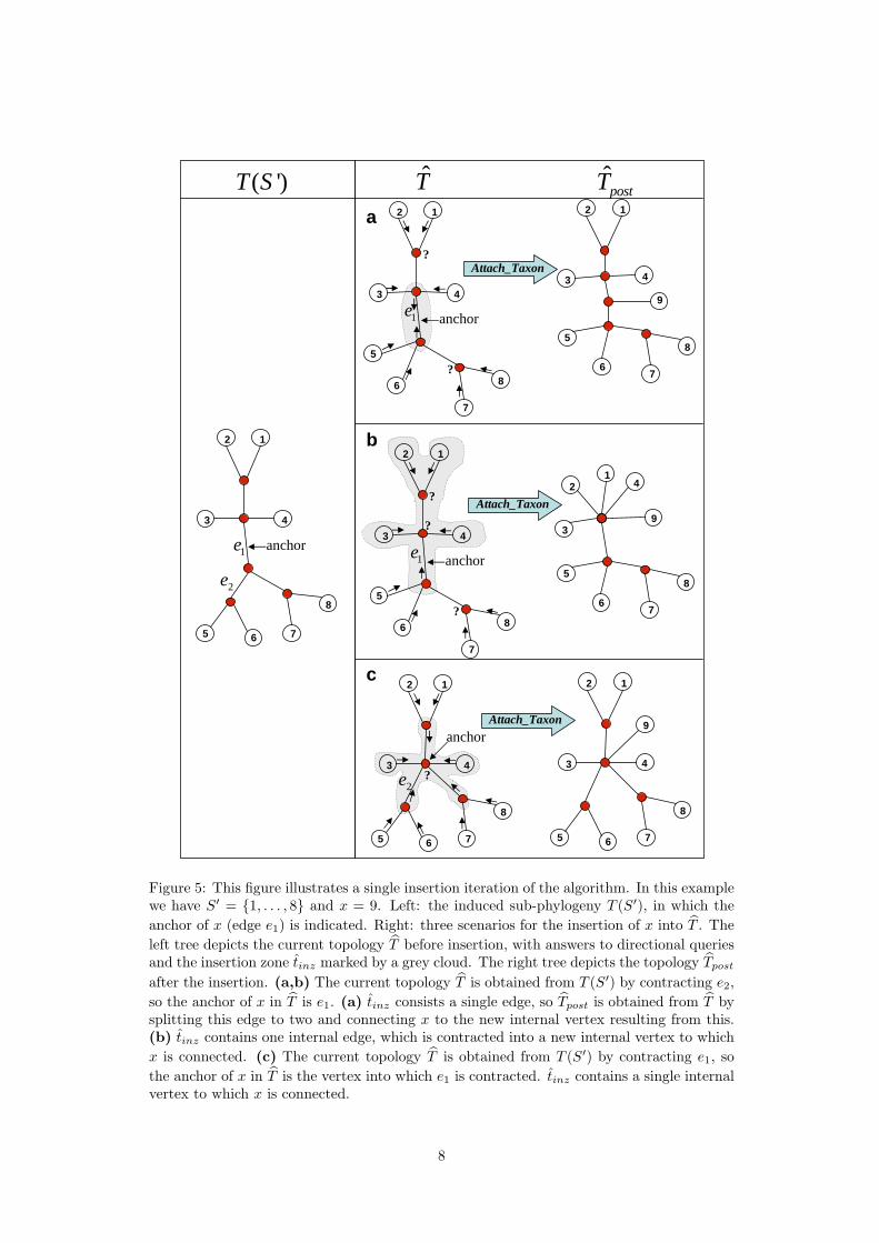
Figure 5: This figure illustrates a single insertion iteration of the algorithm. In this examplewe have S′ = {1, . . . , 8} and x = 9. Left: the induced sub-phylogeny T (S′), in which theanchor of x (edge e1) is indicated. Right: three scenarios for the insertion of x into T . Theleft tree depicts the current topology T before insertion, with answers to directional queriesand the insertion zone tinz marked by a grey cloud. The right tree depicts the topology Tpost

after the insertion. (a,b) The current topology T is obtained from T (S′) by contracting e2,so the anchor of x in T is e1. (a) tinz consists a single edge, so Tpost is obtained from T bysplitting this edge to two and connecting x to the new internal vertex resulting from this.(b) tinz contains one internal edge, which is contracted into a new internal vertex to whichx is connected. (c) The current topology T is obtained from T (S′) by contracting e1, sothe anchor of x in T is the vertex into which e1 is contracted. tinz contains a single internalvertex to which x is connected.

8

Attach_Taxon

43

5

6

7

8

12

4

1

3

5

67

8

2

9

T ˆpost

T

ˆ xT

43

5

6

7

8

9

12

anchor

u

u

v

v

z

z

w

9p

Figure 6: explicit and implicit contractions The insertion of taxon x = 9 into T aspresented in Fig. 5b results in contraction of two edges in T+x into the vertex w in Tpost:An explicit contraction of (u, z) (medium bold) as internal edge of the ε-environment ofx, and an implicit contraction of (u, p9) (bold), which occurs since the anchor of x is theexternal edge (u, v) of tinz.

Lemma 3.7. Let T be a contraction of T (S′) and let x ∈ S\S′. Then the tree Tpost obtainedby Attach Taxon(T , x) is a contraction of T (S′ ∪ {x}).

Proof. The lemma holds trivially if Tpost is obtained by step 2 of the proecedure. It holdsalso when Tpost is obtained by step 3 or 4 due to Observation 3.6 and the fact that, byObservation 3.4(1), anchorbT (x) touches the subtree spanned by internal(tinz).

4 ε-Reliable Directional Oracles.

We now formalize the properties of the partial directional oracle which guarantee that allcontracted edges are of weight smaller than ε.

Definition 4.1 (ε-environment). tenv(T , x, ε), the ε-environment of x in T , is the maximalsubtree of T+x which includes x and whose internal edges have weight at most ε.

Definition 4.2 (ε-reliability). A partial directional oracle PDO is said to be ε-reliable for(T , x), if the insertion zone of x determined by PDO is included in the ε-environment of x,i.e.: V (tinz) ⊆ V (tenv(T , x, ε)). Specifically, any internal vertex of tinz is also an internalvertex of tenv(T , x, ε).

Lemma 4.3. If the partial directional oracle PDO used in the calculation of tinz is ε-reliablefor (T , x), then Tpost is an ε-contraction of T (S′ ∪ {x}).

Proof. By Lemma 3.7, Tpost is a contraction of T (S′ ∪{x}). Hence, by the assumption thatT is an ε-contraction of T (S′), we only need to prove that all the edges contracted duringthe current iteration are of weight smaller than ε. Consider such a contracted edge (u, v).Then each endpoint of e is either an internal vertex of tinz and hence, by Definition 4.2 also

9

of tenv(T , x, ε), or it is px, the parent of x, which by definition is also an internal vertex oftenv(T , x, ε). Thus e is an internal edge of tenv(T , x, ε), and hence its weight is smaller thanε.

Lemma 4.3 provides the main inductive argument used in the proof of our main result(Theorem 6.9). It is important to note that the validity of this argument requires that ourpartial directional oracle is ε-reliable in every iteration of the algorithm.

5 An Efficient Implementation of the Partial DirectionalOracle Using Quartet Queries.

In this section we present our partial directional oracle and give explicit conditions on Tand x under which it is ε-reliable. Our directional oracle PDO uses queries on quartetsplits. A taxon-quartet q = {a, b, c, d} ⊆ S defines an induced sub-topology T (q) which iseither a star or a split (x, y|z, w), where {x, y, z, w} = q, and T (q) has a single internal edge(of positive weight) separating {x, y} from {z, w}. Reconstructing phylogenetic trees fromquartet splits dates back as far as [4]. In order to allow quartet queries over noisy data, weintroduce the concept of a partial quartet oracle, which may fail to return a split when it isnot confident in the result (even when the topology of the quartet is not a star).

Definition 5.1 (Partial Quartet Oracle). Let T be a phylogenetic tree over S. A partialquartet oracle for T is a function which receives a quartet q ⊆ S and returns either the(correct) split of q in T , or ‘null’.

Recall that a partial directional oracle, when queried on a vertex v and taxon x, returnseither ‘null’ or a neighbor u of v which is on the same side of v as x. The procedure describedbelow seeks such a neighbor via a series of queries to a partial quartet oracle PQO. Thesequartet queries include the new taxon x and three other taxa s1, s2, s3 of T which representthree different directions corresponding to three different neighbors of v in T , defined asfollows:

Definition 5.2 (Directional Representatives). Let (u, v) be an edge in T . A taxon s of Tis a directional representative of (v → u) if u ∈ pathbT (v, s). The directional representativeof (v → u) is denoted by sv(u).

Our partial directional oracle contains two main phases:Triplets Tournament: In this phase, the set of all possible directions (represented byNbT (v)) is iteratively screened to end up with at most one candidate direction. In eachiteration a quartet is queried and as a result at least two directions are eliminated from theset of candidates. If the tournament results in an empty candidate set, then the directionaloracle returns ‘null’. Otherwise, the tournament results in a single surviving candidate. Thefollowing validation phase is needed in order to guarantee that the surviving candidate (ifexists) indeed indicates the correct direction.Validation: Validation of the direction represented by the surviving neighbor u is doneby another series of quartet queries which contain both x and sv(u). If all quartet queriespositively validate this direction (meaning that they put x and sv(u) on the same side ofthe split), then u is returned. Otherwise, the directional oracle returns ‘null’.

Claim 5.3. The time required for the execution of PDO(T , v, x) is linear in degbT (v).

Proof. Each iteration of the triplets tournament phase takes O(1) time, and at least twoneighbors of v are eliminated from the candidate set at each iteration. So this phase ends

10

after at most 12degbT (v) iterations. The validation phase simply scans the neighborhood of

v, and so it ends after at most O(degbT (v)) time.

Lemma 5.4. If PQO is a partial quartet oracle for T and all directional representativessatisfy Definition 5.2, then procedure PDO described above is a (truthful) partial directionaloracle for T .

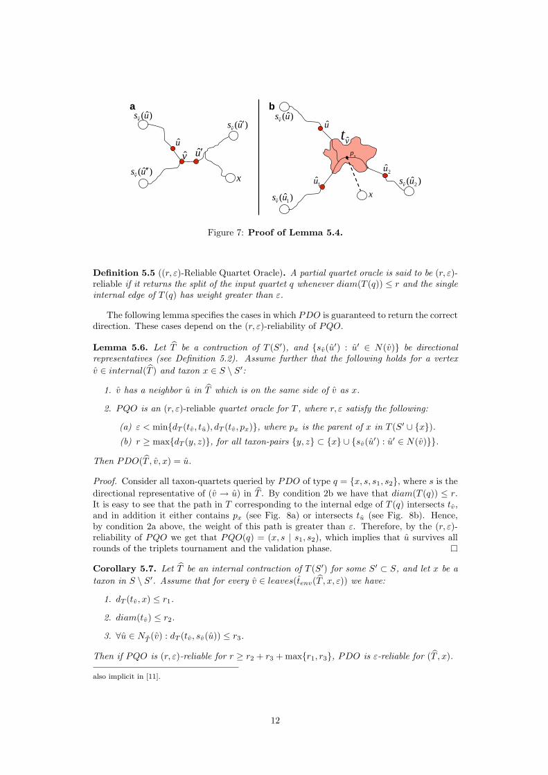
Proof. Consider a valid input instance (T , v, x) for PDO. If v is a taxon, then PDO returnsthe unique neighbor of v in T , as required. So assume v is an internal vertex of T . It issufficient to show that for any vertex u ∈ NbT (v) which is not on the same side of v as x,there exists a vertex which fails u at step 5b of the validation phase. If there is a vertexu′ ∈ N(v) which is on the same side of v as x, then u′ fails the validation of u when choseneither as u2 or as u1 (see Fig. 7a). If there is no such vertex, then v is the anchor of x

in T , and px – the parent of x in T (leaves(T ) ∪ {x}) – is contained in tv. In this case,for each choice of u1 there exists u2 ∈ NbT (v) \ {u, u1} s.t. pathT (px, tu) separates tu1 fromtu2 (see Fig. 7b). This means that the quartet {x, sv(u), sv(u1), sv(u2)} is not split by(x, sv(u)|sv(u1), sv(u2)), and hence the validation of u fails.

The Partial Directional Oracle – PDO(T , v, x):

1. Initialize candidate set C ← NbT (v).

2. If C = {u} (v is a taxon), return u.

3. Otherwise (|C| ≥ 3), proceed as follows:

4. Triplets Tournament:

– While |C| > 1 do:

• If |C| = 2, then C ← C ∪ {u}, for some u ∈ NbT (v) \ C.

• Select some triplet {u1, u2, u3} ⊆ C and invoke PQO({x, sv(u1), sv(u2), sv(u3)}).– If output is ‘null’, then remove u1, u2, u3 from C.– Otherwise, the output is (x, sv(ui) | sv(uj), sv(uk)) (where {i, j, k} = {1, 2, 3}),

then remove uj , uk from C.

– If the tournament results in C = ∅, return ‘null’.

5. Validation: C = {u} for some u ∈ NbT (v).

(a) Select some vertex u1 ∈ NbT (v) \ {u}.(b) For every u2 ∈ NbT (v) \ {u, u1}, invoke PQO({x, sv(u), sv(u1), sv(u2)}).

• If output is (x, sv(u) | sv(u1), sv(u2)), then continue.• Otherwise, stop and return ‘null’.

(c) Return u (if it survived all rounds).

The truthfulness of PDO is not enough: in order to get meaningful results, we need inaddition that in some cases it will return a valid direction (not ‘null’). For this, we need toclasiffy the cases where our partial quartet oracle guarantees to return a valid split. Undermost common models of evolution, the reliability of quartet splits inferred from estimateddistances increases when the diameter of the quartet decreases and the length of the internaledge increases [13, 23, 11]. This motivates the definition of a (r, ε)-reliable quartet oraclebelow1.

1In Section 6 we present an (r, ε)-reliable distance-based quartet oracle. A somewhat similar oracle is

11

vu

x

ˆ ˆ( )vs u

ˆ ˆ( )vs u′′

ˆ ˆ( )vs u′

u′

xˆ 1( )vs u

2u

ˆ 2ˆ( )vs u

xp

uˆ ˆ( )vs u

vt

ba

1u

Figure 7: Proof of Lemma 5.4.

Definition 5.5 ((r, ε)-Reliable Quartet Oracle). A partial quartet oracle is said to be (r, ε)-reliable if it returns the split of the input quartet q whenever diam(T (q)) ≤ r and the singleinternal edge of T (q) has weight greater than ε.

The following lemma specifies the cases in which PDO is guaranteed to return the correctdirection. These cases depend on the (r, ε)-reliability of PQO.

Lemma 5.6. Let T be a contraction of T (S′), and {sv(u′) : u′ ∈ N(v)} be directionalrepresentatives (see Definition 5.2). Assume further that the following holds for a vertexv ∈ internal(T ) and taxon x ∈ S \ S′:

1. v has a neighbor u in T which is on the same side of v as x.

2. PQO is an (r, ε)-reliable quartet oracle for T , where r, ε satisfy the following:

(a) ε < min{dT (tv, tu), dT (tv, px)}, where px is the parent of x in T (S′ ∪ {x}).(b) r ≥ max{dT (y, z)}, for all taxon-pairs {y, z} ⊂ {x} ∪ {sv(u′) : u′ ∈ N(v)}}.

Then PDO(T , v, x) = u.

Proof. Consider all taxon-quartets queried by PDO of type q = {x, s, s1, s2}, where s is thedirectional representative of (v → u) in T . By condition 2b we have that diam(T (q)) ≤ r.It is easy to see that the path in T corresponding to the internal edge of T (q) intersects tv,and in addition it either contains px (see Fig. 8a) or intersects tu (see Fig. 8b). Hence,by condition 2a above, the weight of this path is greater than ε. Therefore, by the (r, ε)-reliability of PQO we get that PQO(q) = (x, s | s1, s2), which implies that u survives allrounds of the triplets tournament and the validation phase.

Corollary 5.7. Let T be an internal contraction of T (S′) for some S′ ⊂ S, and let x be ataxon in S \ S′. Assume that for every v ∈ leaves(tenv(T , x, ε)) we have:

1. dT (tv, x) ≤ r1.

2. diam(tv) ≤ r2.

3. ∀u ∈ NbT (v) : dT (tv, sv(u)) ≤ r3.

Then if PQO is (r, ε)-reliable for r ≥ r2 + r3 + max{r1, r3}, PDO is ε-reliable for (T , x).

also implicit in [11].

12

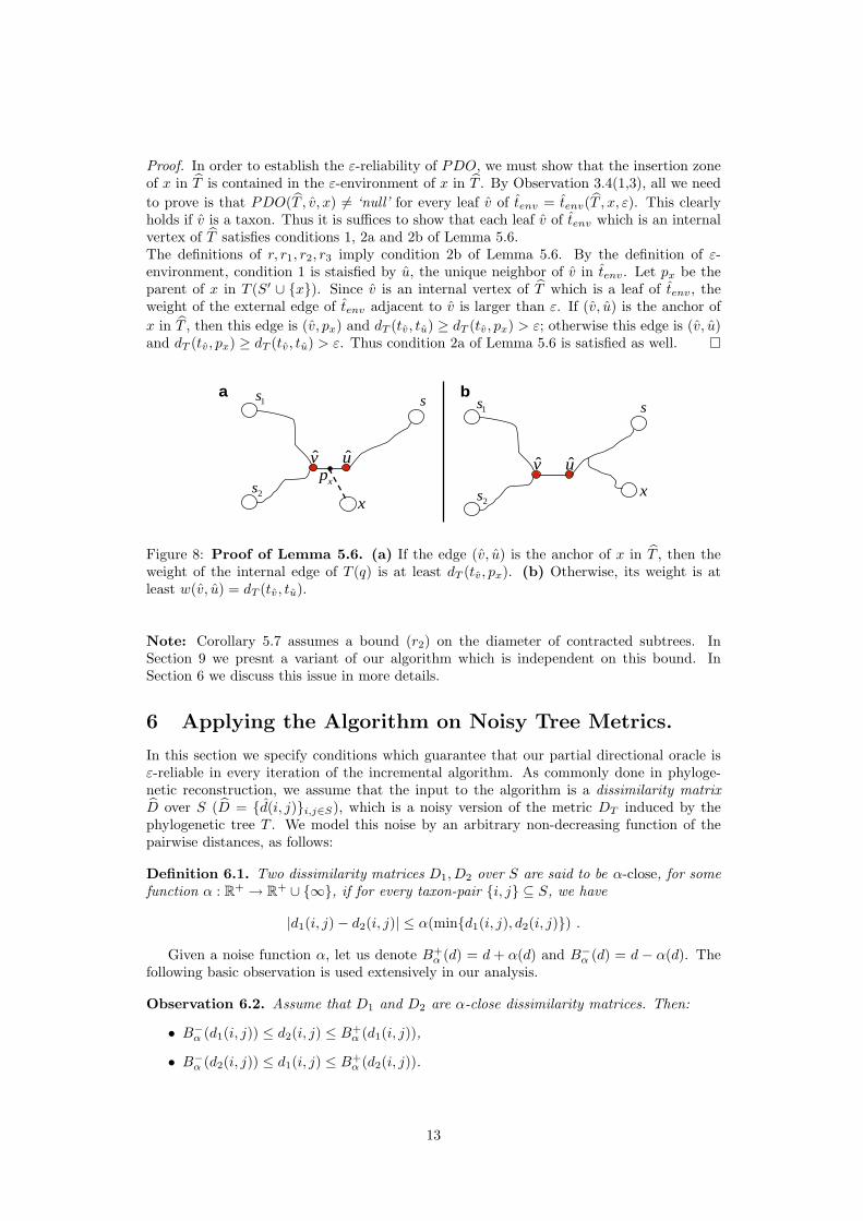
Proof. In order to establish the ε-reliability of PDO, we must show that the insertion zoneof x in T is contained in the ε-environment of x in T . By Observation 3.4(1,3), all we needto prove is that PDO(T , v, x) 6= ‘null’ for every leaf v of tenv = tenv(T , x, ε). This clearlyholds if v is a taxon. Thus it is suffices to show that each leaf v of tenv which is an internalvertex of T satisfies conditions 1, 2a and 2b of Lemma 5.6.The definitions of r, r1, r2, r3 imply condition 2b of Lemma 5.6. By the definition of ε-environment, condition 1 is staisfied by u, the unique neighbor of v in tenv. Let px be theparent of x in T (S′ ∪ {x}). Since v is an internal vertex of T which is a leaf of tenv, theweight of the external edge of tenv adjacent to v is larger than ε. If (v, u) is the anchor ofx in T , then this edge is (v, px) and dT (tv, tu) ≥ dT (tv, px) > ε; otherwise this edge is (v, u)and dT (tv, px) ≥ dT (tv, tu) > ε. Thus condition 2a of Lemma 5.6 is satisfied as well.

v

x

1s s

u

2s

v

x

1ss

u

2sxp

ba

Figure 8: Proof of Lemma 5.6. (a) If the edge (v, u) is the anchor of x in T , then theweight of the internal edge of T (q) is at least dT (tv, px). (b) Otherwise, its weight is atleast w(v, u) = dT (tv, tu).

Note: Corollary 5.7 assumes a bound (r2) on the diameter of contracted subtrees. InSection 9 we presnt a variant of our algorithm which is independent on this bound. InSection 6 we discuss this issue in more details.

6 Applying the Algorithm on Noisy Tree Metrics.

In this section we specify conditions which guarantee that our partial directional oracle isε-reliable in every iteration of the incremental algorithm. As commonly done in phyloge-netic reconstruction, we assume that the input to the algorithm is a dissimilarity matrixD over S (D = {d(i, j)}i,j∈S), which is a noisy version of the metric DT induced by thephylogenetic tree T . We model this noise by an arbitrary non-decreasing function of thepairwise distances, as follows:

Definition 6.1. Two dissimilarity matrices D1, D2 over S are said to be α-close, for somefunction α : R+ → R+ ∪ {∞}, if for every taxon-pair {i, j} ⊆ S, we have

|d1(i, j)− d2(i, j)| ≤ α(min{d1(i, j), d2(i, j)}) .

Given a noise function α, let us denote B+α (d) = d + α(d) and B−

α (d) = d − α(d). Thefollowing basic observation is used extensively in our analysis.

Observation 6.2. Assume that D1 and D2 are α-close dissimilarity matrices. Then:

• B−α (d1(i, j)) ≤ d2(i, j) ≤ B+

α (d1(i, j)),

• B−α (d2(i, j)) ≤ d1(i, j) ≤ B+

α (d2(i, j)).

13

For our analysis we assume that the input matrix D and the tree-metric DT are α-close for some efficiently computable non-decreasing function α. Our partial quartet oracleFPM bD,α(q) is the following modified version of the well-known four-point method (FPM)(see e.g. [13]).

The Partial Quartet Oracle – FPM bD,α(q):Let q = {a, b, c, d}, and assume a labelling of the four taxa which satisfies:

d(a, b) + d(c, d) ≤ min{d(a, c) + d(b, d) , d(a, d) + d(b, c)} .

– Return (a, b|c, d), if:

B−α (d(a, c)) + B−

α (d(b, d)) > B+α (d(a, b)) + B+

α (d(c, d)) (4)

– Otherwise, return ‘null’.

Lemma 6.3. Assume that D is α-close to DT . Then for every r ∈ R+, FPM bD,α is an(r, εr)-reliable partial quartet oracle for T , where εr = 4α(B+

α (r)).

Proof. First we show that FPM bD,α is a truthful quartet oracle, meaning that if the in-equality in §4 holds, then (a, b|c, d) is the correct quartet split in T . This is established byshowing that dT (a, b) + dT (c, d) < dT (a, c) + dT (b, d).

dT (a, b) + dT (c, d) ≤ B+α (d(a, b)) + B+

α (d(c, d))

(by §4) < B−α (d(a, c)) + B−

α (d(b, d)) ≤ dT (a, c) + dT (b, d) .

We are left to show that if (a) T (q) = (a, b|c, d), (b) diam(T (q)) ≤ r, and (c) theweight of the single internal edge in T (q) is larger than εr = 4α(B+

α (r)), then the quartetsplit (a, b|c, d) is returned. Hence we have to prove that (a),(b),(c) imply §4. Notice that (b)implies that d(i, j) ≤ B+

α (r) for all {i, j} ⊂ q. Using the monotonicity of α and Observation6.2 we get:

B−α (d(a, c)) + B−

α (d(b, d)) ≥ d(a, c) + d(b, d)− 2α(B+α (r)) ≥

dT (a, c) + dT (b, d)− 4α(B+α (r)) > (by (a),(c) above)

dT (a, b) + dT (c, d) + 4α(B+α (r)) ≥ d(a, b) + d(c, d) + 2α(B+

α (r)) ≥B+

α (d(a, b)) + B+α (d(c, d)).

Lemma 6.3 establishes the (well known) fact, that in order to establish (r, ε)-reliabilityfor small values of ε, we will have to make sure that the diameters of the quartets queriedby our algorithm are kept as small as possible. For this we select the inserted taxon to beas close as possible to the current topology, and the directional representatives as close aspossible to the corresponding edges, as specified below.

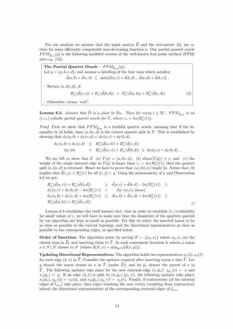
Order of Insertion: The algorithm starts by setting S′ ← {x0, x1} where x0, x1 are theclosest taxa in D, and inserting them to T . In each consequent iteration it selects a taxonx ∈ S \ S′ closest to S′ (where d(S′, x) = miny∈S{d(x, y)}).Updating Directional Representatives: The algorithm holds two representatives sv(u), su(v)for each edge (u, v) in T . Consider the updates required after inserting taxon x into T . Lety denote the taxon closest to x in T (under D), and let px denote the parent of x inT . The following updates take place for the new external edge (x, px): spx(x) ← x andsx(px) ← y. If an edge (u, v) is split to (u, px), (px, v), the following updates take place:sv(px), spx(u) ← sv(u), and su(px), spx(v) ← su(v). Finally, if contractions (of the internaledges of tinz) take place, then edges touching the new vertex (resulting from contraction)inherit the directional representatives of the corresponding external edges of tinz.

14

b d

e g

Attach_Taxon

a b

a

xx y

a

b

ba

b

a

b

c

d

e

f

g

h

Attach_Taxon

a c

f h

xx y

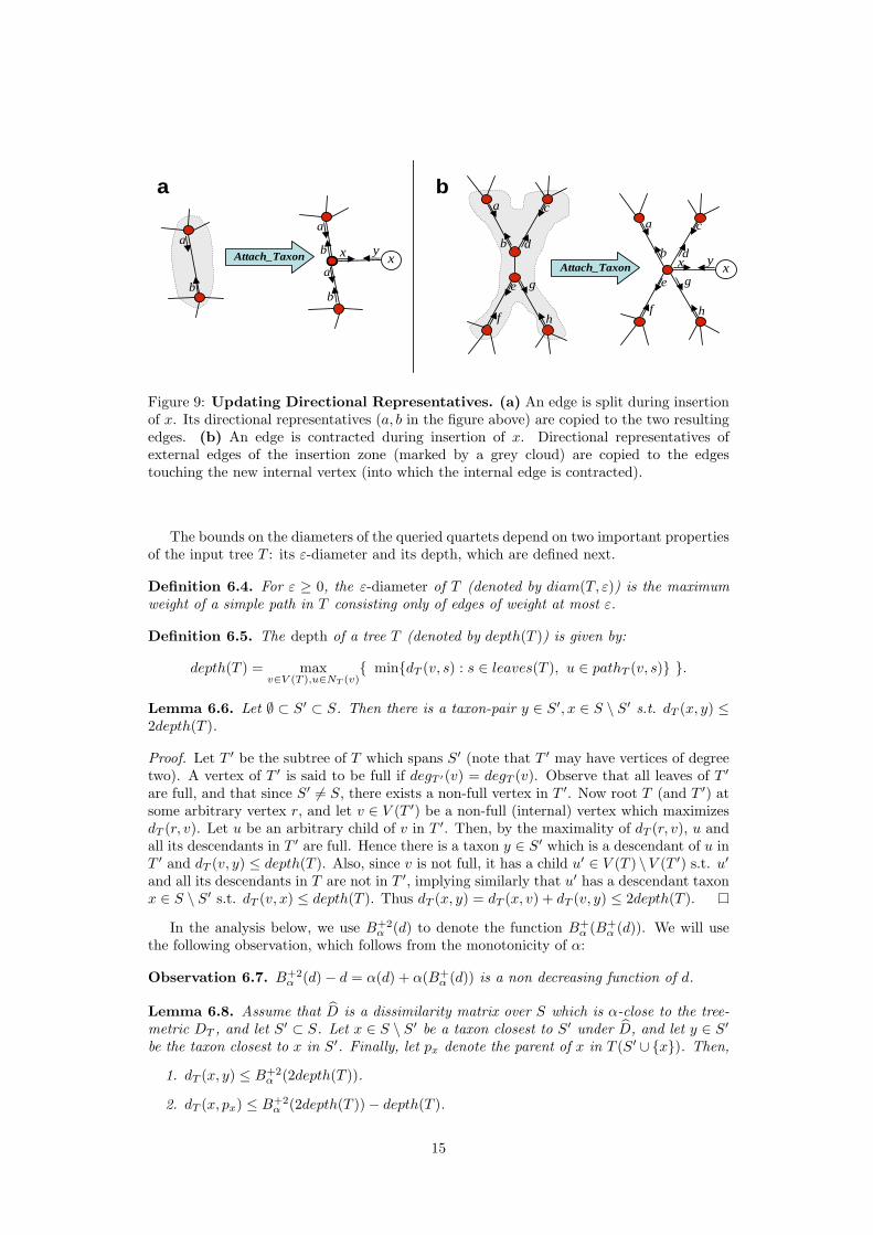
Figure 9: Updating Directional Representatives. (a) An edge is split during insertionof x. Its directional representatives (a, b in the figure above) are copied to the two resultingedges. (b) An edge is contracted during insertion of x. Directional representatives ofexternal edges of the insertion zone (marked by a grey cloud) are copied to the edgestouching the new internal vertex (into which the internal edge is contracted).

The bounds on the diameters of the queried quartets depend on two important propertiesof the input tree T : its ε-diameter and its depth, which are defined next.

Definition 6.4. For ε ≥ 0, the ε-diameter of T (denoted by diam(T, ε)) is the maximumweight of a simple path in T consisting only of edges of weight at most ε.

Definition 6.5. The depth of a tree T (denoted by depth(T )) is given by:

depth(T ) = maxv∈V (T ),u∈NT (v)

{ min{dT (v, s) : s ∈ leaves(T ), u ∈ pathT (v, s)} }.

Lemma 6.6. Let ∅ ⊂ S′ ⊂ S. Then there is a taxon-pair y ∈ S′, x ∈ S \ S′ s.t. dT (x, y) ≤2depth(T ).

Proof. Let T ′ be the subtree of T which spans S′ (note that T ′ may have vertices of degreetwo). A vertex of T ′ is said to be full if degT ′(v) = degT (v). Observe that all leaves of T ′

are full, and that since S′ 6= S, there exists a non-full vertex in T ′. Now root T (and T ′) atsome arbitrary vertex r, and let v ∈ V (T ′) be a non-full (internal) vertex which maximizesdT (r, v). Let u be an arbitrary child of v in T ′. Then, by the maximality of dT (r, v), u andall its descendants in T ′ are full. Hence there is a taxon y ∈ S′ which is a descendant of u inT ′ and dT (v, y) ≤ depth(T ). Also, since v is not full, it has a child u′ ∈ V (T ) \V (T ′) s.t. u′

and all its descendants in T are not in T ′, implying similarly that u′ has a descendant taxonx ∈ S \ S′ s.t. dT (v, x) ≤ depth(T ). Thus dT (x, y) = dT (x, v) + dT (v, y) ≤ 2depth(T ).

In the analysis below, we use B+2α (d) to denote the function B+

α (B+α (d)). We will use

the following observation, which follows from the monotonicity of α:

Observation 6.7. B+2α (d)− d = α(d) + α(B+

α (d)) is a non decreasing function of d.

Lemma 6.8. Assume that D is a dissimilarity matrix over S which is α-close to the tree-metric DT , and let S′ ⊂ S. Let x ∈ S \ S′ be a taxon closest to S′ under D, and let y ∈ S′

be the taxon closest to x in S′. Finally, let px denote the parent of x in T (S′ ∪ {x}). Then,

1. dT (x, y) ≤ B+2α (2depth(T )).

2. dT (x, px) ≤ B+2α (2depth(T ))− depth(T ).

15

Proof. Throughout the proof we extensively apply Observation 6.2 and use depth in short todenote depth(T ). By Lemma 6.6 there exist x′ ∈ S \S′ and y′ ∈ S′ s.t. dT (x′, y′) ≤ 2depth.For such x′, y′ we have d(x′, y′) ≤ B+

α (dT (x′, y′)) ≤ B+α (2depth). Hence, since d(x, y) ≤

d(x′, y′), we get: dT (x, y) ≤ B+α (d(x, y)) ≤ B+

α (d(x′, y′)) ≤ B+2α (2depth).

The second inequality is proved similarly. By the definition of depth there must bea taxon x′ ∈ S \ S′ s.t. dT (px, x′) ≤ depth. Now notice that dT (x, px) − dT (x′, px) =dT (x, y)− dT (x′, y), thus

dT (x, px) = dT (x′, px) + [dT (x, y)− dT (x′, y)] ≤ depth + [dT (x, y)− dT (x′, y)] .

So it suffices to show that dT (x, y) ≤ dT (x′, y)+B+2α (2depth)−2depth. If dT (x′, y) ≥ 2depth,

then this is implied by the fact that dT (x, y) ≤ B+2α (2depth). So assume that dT (x′, y) <

2depth. Then we get:

dT (x, y) ≤ B+α (d(x, y)) ≤ B+

α (d(x′, y)) ≤ B+2α (dT (x′, y))

(by Observation 6.7 above) ≤ dT (x′, y) + B+2α (2depth)− 2depth.

We are now ready to present the main result of this section:

Theorem 6.9. Consider a phylogenetic tree T over a taxon-set S. Let D be a dissimilaritymatrix which is α-close to the tree-induced metric DT , for some non-decreasing function α.Assume that the following holds for some ε ∈ R+:

ε ≥ 4α(B+α (r)) for r = 3B+2

α (2depth(T ))− 2depth(T ) + 2diam(T, ε) . (5)

Then, algorithm Incremental Reconstruct (Section 3) which uses the quartet oracle FPM bD,αreturns a topology which is an ε-contraction of T .

Sketch of Proof. We use depth in short to denote depth(T ), and Hε to denote diam(T, ε). ByLemma 6.3, §5 implies that FPM bD,α is an (r, ε)-reliable quartet oracle for r = 3B+2

α (2depth)−2depth + 2Hε. The proof is completed by proving (inductively) that the topology T ouralgorithm holds throughout its execution satisfies the following properties:

1. T is a ε-contraction of T (S′).

2. Every edge in T has weight at most B+2α (2depth)− depth.

3. For every directional representative sv(u) in T , we have d(tv, sv(u)) ≤ B+2α (2depth).

The induction is pretty straightforward. Lemma 6.8 is used to prove conditions 2 and 3.Condition 1 is proved with Lemma 4.3 and Corollary 5.7, using the induction hypothesis toobtain the following bounds on r1, r2, r3:

r1 = 2B+2α (2depth)− 2depth + Hε / r2 = Hε / r3 = B+2

α (2depth).

The bounds on r2, r3 follow immediately from conditions 1 and 3. The bound on r1 isobtained by observing the path in T (S′ ∪ {x}) connecting x and tv, where v is an arbitraryleaf of tenv: condition 2 implies a bound of B+2

α (2depth)− depth on the weight of the firstand last edges, and the weight of the rest of the path is bounded by Hε since it consists ofedges whose weight is at most ε.

6.1 Guaranteeing Reconstruction of Short Edges

In this section we give a closer look at the weight threshold ε, above which edges in T areguaranteed (correct) reconstruction by our algorithm. Such weight thresholds were providedfor several other algorithms by Atteson in [1] (by what Atteson terms as ‘edge l∞ radius’).However, since Atteson ties this threshold to the worst-case noise, the best threshold his

16

analysis provides is 2α(diam(T )) (achieved e.g. by Buneman’s algorithm [4] and DLCA [17]).To imply (adaptive) fast convergence in common models of evolutions (as will be discussedin Section 8), we need our algorithm to imply a tighter threshold ε = 4α(c · depth(T )))for some constant c. To achieve this stronger threshold, we use the following corrolary ofTheorem 6.9.

Corollary 6.10. Let T, D and α be as in Theorem 6.9. Let ε ∈ R+ be s.t. ε ≥ 4α(r′), wherer′ = 4depth(T ) + 1.75ε + 2diam(T, ε). Then algorithm Incremental Reconstruct (Section 3)returns an ε-contraction of T .

Proof. According to Theorem 6.9, all we need to show is that ε ≥ 4α(B+α (r)) for r =

3B+2α (2depth(T )) − 2depth(T ) + 2diam(T, ε). The fact that ε ≥ 4α(r′) implies that for

every d ≤ r′, we have B+α (d) ≤ d + α(r′) ≤ d + ε

4 . So we get:

2depth(T ) ≤ r′ ⇒ B+α (2depth(T )) ≤ 2depth(T ) +

ε

4≤ r′ ⇒

B+2α (2depth(T )) ≤ 2depth(T ) +

ε

2⇒ r ≤ 4depth(T ) + 1.5ε + 2diam(T, ε) ≤ r′ ⇒

B+α (r) ≤ 4depth(T ) + 1.75ε + 2diam(T, ε) = r′ ⇒ ε ≥ 4α(B+

α (r)) .

Assume that T and ε are such that depth(T ) ≥ 1.75ε + 2diam(T, ε). In this case,Corollary 6.10 implies that our algorithm is guaranteed to correctly reconstruct all edges inT which are longer than ε = 4α(5depth(T )). The above assumption (depth(T ) ≥ 1.75ε +2diam(T, ε)) is likely to hold whenever we are interested (a-priori) in weight-thresholdswhich are not too large (eg, when most of the edges of the tree are of weight larger than ε).In Section 9 we present a modification of our algorithm which gurantees a weight-thresholdof ε ≤ 4α(12depth(T )) for any tree T . Whereas in practice we do not expect the modifiedalgorithm to perform much better than the original one, its significance is in being adaptivefast convergent (see discussion in Section 8).

7 Complexity Analysis.

The space complexity of the algorithm (disregarding the space needed for storing the inputdissimilarity matrix D) is obviously linear in n (the number of taxa), since the currenttopology T and the directional representatives can easily be maintained in linear spacethroughout the algorithm. The time complexity of the algorithm is quadratic, which isasymptotically optimal for algorithms reconstructing a phylogenetic tree with unboundedvertex-degrees, even from the exact tree-induced metric (see [10]). Each iteration involvesselecting a taxon for insertion and applying Attach Taxon. Note that computing the nexttaxon to be inserted (the one closest to S′) can be done in linear time as in Dijkstra MSTalgorithm [6]. The most time consuming task in Attach Taxon is computing the insertionzone. This can be done by querying the directional oracle on all vertices of T , and thenpruning T in a DFS-traversal according to the queries’ results. The DFS-traversal andpruning is clearly linear in n. By Claim 5.3, the total time complexity of all queries to thedirectional oracle PDO is linear in the sum of vertex-degrees, which is also linear in n.

8 Reliable Reconstruction from Biological Sequences.

In this section we study the inter-taxa distances and the noise function induced by a stochas-tic process of sequence evolution. Since the model is stochastic, the resulting noise functionα will be ‘probabilistic’ in the sense that it bounds the noise only with sufficiently high prob-ability. We then use this noise function together with the results of Section 6 to establishthe (inverse) relation between the input sequence length and weights of contracted edges.

17

8.1 Stochastic Model of Evolution

The results presented in this section assume the Cavender-Farris-Neyman [5, 15, 25] (CFN)model of binary sequence evolution, but they may be generalized to more complex modelsas well. The CFN model assumes a rooted tree T , whose edges are associated with sym-metric changing probabilities {pe}e∈E(T ). The process of evolution is modelled by uniformlyrandomizing a binary state (0 or 1) at the root and propagating mutations along the treeedges according to their changing probabilities. A site is defined by the n random statesgenerated by the above process at the leaves of the tree. Note that under a given model-tree,the probability distribution of a specific site is well defined. Repeating this process k times(independently), yields n binary sequences of length k (corresponding to k sites), which mayserve as input to a phylogenetic reconstruction method.

The (additive) metric DT induced by the model-tree T is defined by assigning the fol-lowing weight to each edge e in T : we = − 1

2 ln(1 − 2pe)2. For u, v ∈ V (T ), denote by puv

the compound changing probability between u and v, which is the probability of observingdifferent states in u and v. The corresponding tree metric DT is given by the followingequality:

dT (u, v) =∑

e∈path(u,v)

we = − 12

ln(1− 2puv) .

Given a pair of sequences (of length k) corresponding to taxa i, j, the observed compoundchanging probability pij is estimated by the normalized hamming distance (i.e. the numberof sites in the two sequences with different states divided by k). The observed pairwisedissimilarities are defined accordingly – d(i, j) = − 1

2 ln(1 − 2pij). Our analysis is largelybased on the following result:

Theorem 8.1. Let DT be a metric induced by a phylogenetic tree T , and let D be anobserved pairwise-dissimilarity matrix derived (as described above) from length-k sequenceswhich evolved along T . Then with probability greater than 1 − 1

n , D and DT are αk-close,where αk is given by:3

αk(d) = − 12

ln

[1− e2d

√6 ln(n)

k

].

In Section 8.2 we provide a proof for this theorem, and in Section 8.3 we discuss itsimplication on the (adaptive) fast convergence of our algorithm.

8.2 A Noise Bound for the CFN Model

In bounding the noise for the CFN model, we concentrate on proving the following result:

Lemma 8.2. For any δ > 0, let αk,δ be defined as follows:

αk,δ(d) = −12

ln

[1− e2d

√2k

ln(

2δ

)]. (6)

Then the tree-induced metric DT and the observed dissimilarity matrix D are αk,δ-close withprobability larger than 1− (

n2

)δ.

Note that Theorem 8.1 is obtained from Lemma 8.2 by substituting δ = 2n3 . This lemma

is proved by bounding the deviation of the observed dissimilarities from the tree-induceddistances (see Lemma 8.4). The bound on this deviation follows the following basic bound,implied by Hoeffding’s inequality.

2When assuming that the changes obey a Poisson distribution, this weight is the expected number ofchanges that occured along e - see e.g. discussion in [16] pp. 156-157

3we use the convention that for z ≤ 0, ln(z) = −∞.

18

Lemma 8.3 ([26], Theorem 4.5). Let X1, . . . , Xk be independent random variables which

get the value 1 with probability p and 0 with probability 1− p, and let Xk =Pk

i=1 Xi

k . Thenfor every λ > 0,

Pr(Xk − p > λ

)≤ exp(−2kλ2) (7)

Pr(Xk − p < −λ

)≤ exp(−2kλ2) (8)

It is not hard to see that for every taxon-pair i, j, pij (as defined in Section 8.1) is anaverage of k random variables satisfying Lemma 8.3. Hence, the deviation of pij from itsexpected value pij can be bounded using this lemma. Lemma 8.4 below translates thisdeviation to the deviation between tree-induced distances and observed dissimilarities.

Lemma 8.4. Let d be the tree-induced distance between two taxa, and let d be the observeddissimilarity between these two taxa. Then for any β > 0 we have:

Pr(d− d > β

)≤ exp

(−k

2(e2β − 1)2

e4d

)(9)

Pr(d− d < −β

)≤ exp

(−k

2(1− e−2β)2

e4d

). (10)

Proof. Let p, p be the real and observed compound changing probabilities between the twotaxa mentioned in the lemma. First we establish §9:

Pr(d− d > β

)= Pr

(12

ln(

1− 2p

1− 2p

)> β

)=

Pr(

1− 2p

1− 2p> e2β

)=

Pr(

1 + 2p− p

1− 2p> e2β

)=

Pr(

p− p >12(e2β − 1)(1− 2p)

)=

Pr(

p− p >12(e2β − 1)e−2d

). (11)

The inequality in §9 is now obtained by plugging λ = 12 (e2β − 1)e−2d in §8. The inequality

in §10 is similarly obtained by first showing (as in §11) that:

Pr(d− d < −β

)= Pr

(p− p <

12(e−2β − 1)e−2d

), (12)

and then plugging λ = 12 (1− e−2β)e−2d in §7.

Note that the bounds we get in §9 and in §10 are not identical: the RHS of §10 is greaterthan the RHS of §9, because β > 0 implies that 1 − e−2β < e2β(1 − e−2β) = e2β − 1.Hence we get:

Pr(|d− d| > β

)< 2 exp

(−k

2(1− e−2β)2

e4d

). (13)

The bound in §14 below is obtained by noticing that d and d are interchangeable in theproof of Lemma 8.4:

Pr(|d− d| > β

)< 2 exp

(−k

2(1− e−2β)2

e4 min{d,d}

). (14)

19

Proof of Lemma 8.2: The noise function αk,δ defined in §6 is obtained by extracting thevalue of β for which the RHS of §13 equals δ. Hence for every taxon pair i, j ∈ S, we getthe following inequality by plugging in αk,δ(min{d(i, j), d(i, j)}) as β in §14:

Pr(|d(i, j)− d(i, j)| > αk,δ( min{d(i, j) , d(i, j)} )

)< δ . (15)

Now, by applying a simple union bound, we get that DT and D are αk,δ-close with proba-bility at least 1− (

n2

)δ.

8.3 Sequence Length Requirements

By combining Theorems 8.1 and 6.9 we are able to establish the relation between k and theweight of edges our algorithm contracts.

Theorem 8.5. Let D be a dissimilarity matrix obtained from n binary taxon-sequences oflength k which evolved according to the CFN model along a phylogenetic tree T . Let ε ∈ R+

be s.t.ε ≥ 4αk

(B+

αk(3B+2

αk(2depth(T ))− 2depth(T ) + 2Hε)

)(16)

(where αk is as defined in Theorem 8.1 and Hε = diam(T, ε)).Then when executed on D, algorithm Incremental Reconstruct (Section 3) returns an ε-contraction of T with probability larger than 1− 1

n .

Proof. This theorem is a direct result of Theorems 6.9 and 8.1

Theorem 8.5 states a condition which allows us to calculate, for a given tree T and inputsequence length k, an upper bound ε on the weight of edges our algorithm contracts. Thefollowing lemma provides a more explicit (but less tight) connection between k and ε.

Corollary 8.6. Let ε ∈ R+, and assume that the sequence length satisfies:

k ≥ 24 ln(n) · e16depth(T )+8ε+8Hε

ε2. (17)

Then algorithm Incremental Reconstruct returns an ε-contraction of T with high probability.

Proof. Corollary 6.10 implies that it is sufficient to show that ε ≥ 4αk(r′) for r′ = 4depth(T )+1.75ε + 2Hε. By plugging in αk as defined in Theorem 8.1, we get that this is equivalent torequiring:

k ≥ 6 ln(n) · e16depth(T )+7ε+8Hε

(1− e−

ε2)2 . (18)

So we are left to show that §17 implies §18. This is established by showing that

4eε

ε2≥ (

1− e−ε2)−2

. (19)

Substituting ε = 2t, §19 is equivalent to e2t

t2 ≥ (1− e−t)−2 , or by taking square root toet

t ≥ (1− e−t)−1 , which is equivalent to the well known inequality et − 1 ≥ t.

Theorem 8.7. Algorithm Incremental Reconstruct is fast converging.

Proof. The proof rather straightforwardly follows from Corollary 8.6. In order to establishfast convergence, we need to prove that our algorithm reconstructs the correct topology of Twith high probability from sequences of poly(n) length, when edge-weights of T are assumedto be within some interval [f, g] (see §2). Applying Corollary 8.6 with any 0 < ε < f ,implies that our algorithm returns the correct topology with high probability, whenever k >24f2 ln(n) · exp(16depth(T ) + 8f)). As mentioned already in Section 1, depth(T ) ≤ g log2(n),which gives us the desired polynomial-bounded on the required sequence length.

20

Note that our algorithm is also absolute fast converging since its input (consisting of Dand the sequence length k) does not require any knowledge about the originating tree.

For adaptive fast convergence we need that sequences of length k = exp(depth(T ))ε2 suffice

to guarantee correct reconstruction (w.h.p.) of all edges of weight greater than ε (see §3).Hence Corollary 8.6 implies adaptive fast convergence only when diam(T, ε) = O(depth(T )).As mentioned in Section 6.1, this restriction is likely to hold in most “normal looking” trees(which do not have large clusters of short edges). However, for our algorithm to be adaptivefast convergent we need to remove this restriction. This is done in the next section.

9 Eliminating Dependence on the Diameter of Con-tracted Subtrees.

In this section we present an alternative insertion procedure which does not depend onthe diameter of contracted subtrees. For this we gurantee that the algorithm queries onlyquartets whose diameter is bounded by some linear function of depth(T ). In our discussionwe focus on a single insertion iteration in which taxon x is inserted into the current topologyT spanning taxon set S′. The main idea behind this alternative insertion procedure is tocompute the insertion zone over a sub-phylogeny induced by a subset S′′ ⊆ S′ containingonly taxa which are close to x. This approach is justified by Lemmas 9.1 and 9.2.

Lemma 9.1. Assume that T (S′′) is an internal contraction of T (S′′) and that PQO is(r, ε)-reliable for r = diam(T (S′′ ∪ {x})). Then PDO is ε-reliable for (T (S′′), x).

Proof. This lemma is directly implied by Lemma 5.6 and the discussion following it.

Lemma 9.2. Let T be an internal contraction of T (S′), and Let S′′ ⊆ S′. Then

1. T (S′′) , the subtree of T induced by S′′, is an internal contraction of T (S′′).

2. An edge (u, v) ∈ E(T (S′′)) is contracted into a vertex v of T (S′′) iff all the edges inpathT (S′)(u, v) are contracted into v in T .

Sketch of Proof. We prove the lemma for the case where S′′ = S′ \ {s} (the general casefollows by induction on |S′ \S′′|). To prove 1, we show that T (S′′) is an internal contractionof T (S′′) by mapping each internal vertex v of T (S′′) onto a subtree t′′v of T (S′′), as follows.Consider an arbitrary vertex v ∈ internal(T ), and the subtree tv of T (S′) contracted intoit in T . If V (tv) ⊆ V (T (S′′)), then tv is also a subtree of T (S′′), and t′′v = tv. If thisis not the case, then tv must contain ps, the parent of s in T (S′) (since ps is the onlypossible vertex in internal(T (S′)) \ internal(T (S′′))). Furthermore, in this case we musthave that degT (S′)(ps) = 3, and NT (S′)(ps) = {s, u, v} for some edge (u, v) ∈ E(T (S′′)) (and(u, ps), (ps, v) ∈ E(T (S′)). There are three possible cases:

1. tv contains neither (u, ps) nor (ps, v), in which case V (tv) = {ps}, and v /∈ V (T (S′′)).

2. tv contains exactly one of the edges (u, ps), (ps, v) - w.l.o.g. it is (u, ps). Then t′′v =tv \ {(u, ps)}.

3. tv contains both (u, ps) and (ps, v), in which case t′′v = tv \ {(u, ps), (ps, v)} ∪ {(u, v)}.

2 is implied by the fact that the edge (u, v) of T (S′′) is contracted in T (S′′) only in thethird case.

In order to use the reduced subset S′′ in the insertion of x into T , we need the ε-reliabilityof PDO for (T (S′′), x) (guaranteed by Lemma 9.1) to translate also to T . This is obtainedby making sure that the anchor of x in T (S′′) is the same as its anchor in T (to be proved

21

in Theorem 9.7). To achieve this, we require S′′ to preserve the anchor of x in T (S′), asspecified by the following definitions and results.

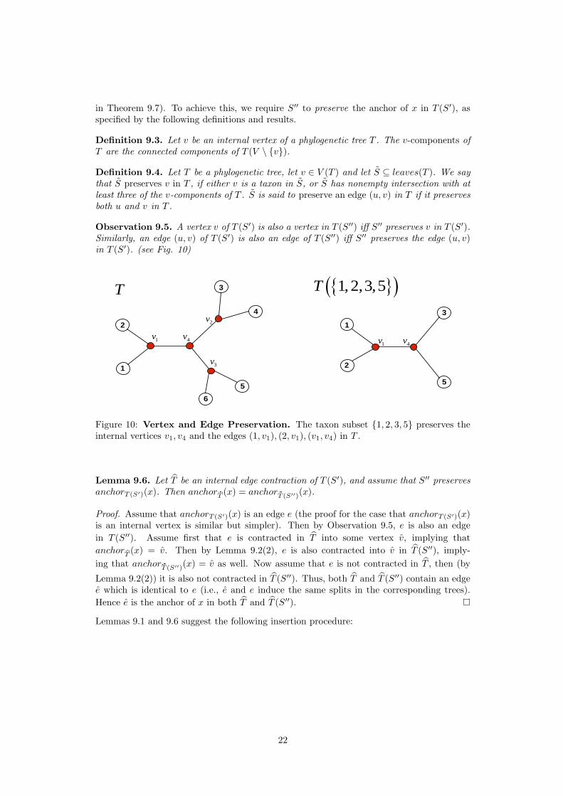
Definition 9.3. Let v be an internal vertex of a phylogenetic tree T . The v-components ofT are the connected components of T (V \ {v}).

Definition 9.4. Let T be a phylogenetic tree, let v ∈ V (T ) and let S ⊆ leaves(T ). We saythat S preserves v in T , if either v is a taxon in S, or S has nonempty intersection with atleast three of the v-components of T . S is said to preserve an edge (u, v) in T if it preservesboth u and v in T .

Observation 9.5. A vertex v of T (S′) is also a vertex in T (S′′) iff S′′ preserves v in T (S′).Similarly, an edge (u, v) of T (S′) is also an edge of T (S′′) iff S′′ preserves the edge (u, v)in T (S′). (see Fig. 10)

3

4

2

1

5

6

4v

T

1

2

3

5

{ }( )1,2,3,5T

1v

2v

1v 4v

3v

Figure 10: Vertex and Edge Preservation. The taxon subset {1, 2, 3, 5} preserves theinternal vertices v1, v4 and the edges (1, v1), (2, v1), (v1, v4) in T .

Lemma 9.6. Let T be an internal edge contraction of T (S′), and assume that S′′ preservesanchorT (S′)(x). Then anchorbT (x) = anchorbT (S′′)(x).

Proof. Assume that anchorT (S′)(x) is an edge e (the proof for the case that anchorT (S′)(x)is an internal vertex is similar but simpler). Then by Observation 9.5, e is also an edgein T (S′′). Assume first that e is contracted in T into some vertex v, implying thatanchorbT (x) = v. Then by Lemma 9.2(2), e is also contracted into v in T (S′′), imply-ing that anchorbT (S′′)(x) = v as well. Now assume that e is not contracted in T , then (by

Lemma 9.2(2)) it is also not contracted in T (S′′). Thus, both T and T (S′′) contain an edgee which is identical to e (i.e., e and e induce the same splits in the corresponding trees).Hence e is the anchor of x in both T and T (S′′).

Lemmas 9.1 and 9.6 suggest the following insertion procedure:

22

Procedure Attach Taxon revised(T , x):

1. Calculate a subset S′′ ⊆ S′, s.t. diam(T (S′′ ∪ {x})) is small, and S′′ preservesthe anchor of x in T (S′).

2. t′′inz ← tinz(T (S′′), x, PDO).

3. If t′′inz is a single edge (u, v), then attach x to T by introducing a new internalvertex px and replacing (u, v) with the three edges (u, px), (v, px), (x, px).

4. If t′′inz has a single internal vertex v (i.e. V (t′′inz) = N(v) ∪ {v}), then add to Tthe edge (v, x).

5. Else (i.e. t′′inz has at least one internal edge), contract into a new vertex v alledges in T which lie on paths corresponding to internal edges of t′′inz, and add toT the edge (v, x).

Implementation note: Before computing the insertion zone in step 2, the algorithmconstructs T (S′′) and determines all directional representatives. Since directional repre-sentatives have to be taxa in S′′, they are not kept from one iteration to the next. Theconstruction of T (S′′) (including calculation of directional representatives) may be achievedin linear time using two DFS scans of T .

Theorem 9.7. Assume that T is an ε-contraction of T (S′), and let Tpost be the topologyresulting from Attach Taxon revised(T , x). Then if S′′ preserves the anchor of x in T (S′)and PDO is ε-reliable for (T (S′′), x), then Tpost is an ε-contraction of T (S′ ∪ {x}).

Proof. If t′′inz consists of a single edge (u, v), then all we need to show is that (u, v) isthe anchor of x in T : This holds since by Observation 3.4(1), anchorbT (S′′)(x) = (u, v),and by Lemma 9.6 anchorbT (x) = anchorbT (S′′)(x). So assume t′′inz contains some internal

vertices. We prove first that if T is an internal contraction of T (S′), then Tpost is an internalcontraction of T (S′ ∪ {x}). For this, let t be the subtree of T spanned by internal(t′′inz).Then Tpost is obtained by contracting t into a new vertex v and attaching x to v. Hence,by Observation 3.6, it suffices to show that anchorbT (x) touches t. This last claim holdssince anchorbT (x) = anchorbT (S′′)(x) (lemma 9.6) and anchorbT (S′′)(x) touches t in T (S′′)(Observation 3.4(1)).

It remains to prove that all the contracted edges are of weight at most ε. Consideran edge e of T (S′ ∪ {x}) which is contracted in Tpost. If e was contracted already in T

then (by our assumption on T ) w(e) ≤ ε. Otherwise, by the ε-reliability of PDO for(T (S′′), x), e must lie on a path corresponding to an internal edge e′ of tenv(T (S′′), x, ε),and w(e) ≤ w(e′) ≤ ε.

We are left to show how to find a reduced subset of taxa S′′ s.t. T (S′′∪{x}) has a smalldiameter and S′′ preserves the anchor of x in T (S′). We assume, as in Section 6, that thealgorithm has access to a dissimilarity matrix D which is α-close to the tree-induced metricDT . We also assume the insertion order suggested in Section 6. Let S′i be the set of attachedtaxa in the beginning of the ith iteration, and let xi /∈ S′i be the taxon chosen for insertionat that stage. Then there is a taxon yi ∈ S′i s.t. d(xi, yi) = min{d(x′, y′) : x′ /∈ S′i, y

′ ∈ S′i}.Our definition of S′′ relies on the following observation (which can be proved by inductionon i):

Observation 9.8. Let di = maxj≤i{d(xj , yj)}. Then depth(T (S′i ∪ {xi})) ≤ Bα(di).

23

Lemma 9.9. Consider the ith iteration in which taxon x = xi is inserted into T (whereS′ = leaves(T )). Then the following set preserves the anchor of x in T (S′):

S′′ ={

s ∈ S′ : d(x, s) ≤ B+α

(3B+

α (di))}

Proof. Assume that the anchor of x in T (S′) is an edge (u, v) (the other case is provedsimilarly). Then we need to show that S′′ preserves both u and v in T (S′). We will showw.l.o.g. that it preserves v. This is done by proving that each v-component of T (S′) containsa taxon s s.t. d(x, s) ≤ B+

α

(3B+

α (di)). Notice that each v-component contains a taxon s

s.t. dT (v, s) ≤ depth(T (S′)). By decomposing path connecting x and s in T (S′ ∪ {x}) into3 parts we get:

dT (x, s) ≤ w(x, px) + w(px, v) + dT (v, s) ≤ 3depth(T (S′ ∪ {x})) ≤ 3B+α (di) .

The lemma then follows since d(x, s) ≤ B+α (dT (x, s)).

The final part left in the analysis is to bound the diameter of T (S′′ ∪{x}). Let s1, s2 betwo arbitrary taxa in S′′. Then d(x, s1), d(x, s2) ≤ B+

α

(3B+

α (di)), and we get:

dT (s1, s2) ≤ dT (s1, x) + dT (s2, x) ≤ B+α (d(s1, x)) + B+

α (d(s2, x)) ≤ 2B+2α

(3B+

α (di))

(20)

Now, Lemma 6.8(1) implies that di ≤ B+α (2depth(T )) in every iteration of the algorithm.

This gives us the following bound:

diam(T (S′′ ∪ {x})) ≤ 2B+2α

(3B+2

α (2depth(T )))

. (21)

We conclude this section by outlining the adjustment of the the main results from Sec-tions 6 and 8 to the case when Attach Taxon revised is used in each iteration of Incremen-tal Reconstruct.

Theorem 9.10. Consider a phylogenetic tree T over a taxon-set S. Let D be a dissimilaritymatrix which is α-close to the tree-induced metric DT , for some non-decreasing function α.Then the modified algorithm returns a topology which is an ε-contraction of T where

ε = 4α(B+

α

(2B+2

α

(3B+2

α (2depth(T )))))

. (22)

Proof. We show (by induction) that in every iteration of the algorithm, the current topologyT is an ε-contraction of T (S′). Consider an arbitrary iteration where x is inserted into T(which is assumed to be an ε-contraction of T (S′)). Let S′′ be the reduced subset calculatedby Attach Taxon revised (as defined in Lemma 9.9). The definition of ε and the boundestablished on diam(T (S′′ ∪ {x})) imply by Lemma 6.3 that FPM bD,α is an (r, ε)-reliablequartet oracle for r = diam(T (S′′ ∪ {x})). And so by Lemma 9.1, PDO is an ε-reliabledirectional oracle for (T (S′′), x). Hence, from Theorem 9.7 (together with Lemma 9.9) weget that Tpost is an ε-contraction of T (S′ ∪ {x}).Adjusting Theorem 9.10 to the probabilistic setting of Section 8 yields the following:

Theorem 9.11. Let D be a dissimilarity matrix obtained from n binary taxon-sequencesof length k which evolved according to the CFN model along a phylogenetic tree T . Thenwhen executed on D, the modified algorithm returns with probability larger than 1 − 1

n anε-contraction of T , where

ε = 4αk

(B+

αk

(2B+2

αk

(3B+2

αk(2depth(T ))

))). (23)

We now turn to prove the adaptive fast convergence of the modified algorithm. Toestablish this we have to determine the sequence length k required for correct reconstructionof edges whose weight is greater than ε. First we simplify equation §23 similarly to the wayCorollary 6.10 simplifies equation §5.

24

Lemma 9.12. Let ε ∈ R+ be s.t. ε ≥ 4α(12depth(T ) + 17

4 ε), then

ε ≥ 4α(B+

α

(2B+2

α

(3B+2

α (2depth(T )))))

.

Proof. Similar to the proof of Corollary 6.10.

Theorem 9.13. The incremental algorithm using Attach Taxon revised is adaptive fastconverging.

proof outline. In order to establish adaptive fast convergence it is enough to show thatassuming edge weights in T are not greater than g, sequences of length k = nO(g)

ε2 aresufficient for the modified algorithm to return (w.h.p.) an ε-contraction of T (see §3).According to Theorem 9.11 and Lemma 9.12, ε contraction is guaranteed w.h.p. if ε ≥4αk

(12depth(T ) + 17

4 ε). Using similar arguments to the ones used in the proof of Corollary

8.6, we get that this is ensured whenever:

k ≥ 24 ln(n) · e48depth(T )+18ε

ε2. (24)

Now assuming g is an upper bound on edge weights, we have depth(T ) ≤ g log2(n) andw.l.o.g. ε ≤ g (otherwise all edge weights are smaller than ε, and hence any execution ofour algorithm outputs an ε-contraction of T ). Hence the required sequence length is smallerthan

24 ln(n) · n48g log2 e · e18ε

ε2=

nO(g)

ε2,

as required.

Acknowledgement:

The first author would like to thank Elchanan Mossel for a very helpful discussion at theearly stages of this research.

References

[1] K. Atteson. The performance of neighbor-joining methods of phylogenetic reconstruc-tion. Algorithmica, 25:251–278, 1999.

[2] V. Berry and D. Bryant. Faster reliable phylogenetic analysis. In RECOMB ’99:Proceedings of the third annual international conference on Computational molecularbiology, pages 59–68, 1999.

[3] W. Beyer, M. Singh, T. Smith, and M. Waterman. Additive evolutionary trees. J TheorBiol, 64(2):199–213, January 1977.

[4] P. Buneman. The recovery of trees from measures of dissimilarity. Mathematics in theArcheological and Historical Sciences, pages 387–395, 1971.

[5] J. Cavender. Taxonomy with confidence. Math Biosci, 40:271–280, 1978.

[6] T. Cormen, C. Leiserson, R. Rivest, and C. Stein. Introduction to Algorithms. MITP,2001. 2nd edition.

[7] M. Cryan, L. Goldberg, and P. Goldberg. Evolutionary trees can be learned in poly-nomial time in the two-state general markov model. SIAM Journal on Computing,31(2):375–397, 2001.

[8] M. Csuros. Fast recovery of evolutionary trees with thousands of nodes. Journal ofComputational Biology, 9(2):277–297, 2002.

25

[9] M. Csuros and M. Kao. Recovering evolutionary trees through harmonic greedy triplets.In SODA: ACM-SIAM Symposium on Discrete Algorithms, pages 261–270, 1999.

[10] J. Culberson and P. Rudnicki. A fast algorithm for constructing trees from distancematrices. Information Processing Letters, 30(4):215–220, February 1989.

[11] C. Daskalakis, C. Hill, A. Jaffe, R. Mihaescu, E. Mossel, and S. Rao. Maximal accurateforests from distance matrices. In RECOMB ’06: Proceedings of the tenth annualinternational conference on Computational molecular biology, pages 281–295, 2006.

[12] C. Daskalakis, E. Mossel, and S. Roch. Optimal phylogenetic reconstruction. In STOC’06: Proceedings of the thirty-eighth annual ACM symposium on Theory of computing,pages 159–168, 2006.

[13] P. Erdos, M. Steel, L. Szekely, and T. Warnow. A few logs suffice to build (almost) alltrees (I). Random Structures and Algorithms, 14:153–184, 1999.

[14] P. Erdos, M. Steel, L. Szekely, and T. Warnow. A few logs suffice to build (almost) alltrees (II). Theoretical Computer Science, 221:77–118, 1999.

[15] J. Farris. A probability model for inferring evolutionary trees. Systematic Zoology,22:250–256, 1973.

[16] J. Felsenstein. Inferring Phylogenies. Sinauer Associated, Inc., Sunderland, MA, 2004.

[17] I. Gronau and S. Moran. Neighbor joining algorithms for inferring phylogenies viaLCA-distances. Journal of Computational Biology, 14(1):1–15, 2007.

[18] D. Huson, S. Nettles, and T. Warnow. Disk-Covering, a fast-converging method forphylogenetic tree reconstruction. J Comp Biol, 6:369–386, 1999.

[19] T. Jukes and C. Cantor. Evolution of protein molecules. In H.N. Munro, editor,Mammalian Protein Metabolism, pages 21–132. Academic Press, New York, 1969.

[20] V. King, L. Zhang, and Y. Zhou. On the complexity of distance-based evolutionarytree reconstruction. In SODA: ACM-SIAM Symposium on Discrete Algorithms, pages444–453, 2003.

[21] B. Moret, K. St. John, and T. Warnow. Absolute convergence: true trees from shortsequences. In SODA: ACM-SIAM Symposium on Discrete Algorithms, pages 186–195,2001.

[22] E. Mossel. Phase transitions in phylogeny. Trans Amer Math Soc, 356:2379–2404, 2004.

[23] E. Mossel. distorted metrics on trees and phylogenetic forests. ACM Transactions oncomputational biology and bioinformatics, 4:108–116, 2007.

[24] E. Mossel and M. Steel. How much can evolved characters tell us about the tree thatgenerated them?, chapter 14. 2005.

[25] J. Neymann. Molecular studies of evolution: A source of novel statistical problems. InS. Gupta and Y. Jackel, editors, Statistical Decision Theory and Related Topics, pages1–27. Academic Press, New York, 1971.

[26] L. Wasserman. All of Statistics. Springer, New York, 2004.

26