illustrating the history of the...

Illustrating the History of the Planimeter

Charles Care0107553

Supervisor: Dr Steve Russ2003-2004

Copy II

Abstract

An analogue device that can perform mathematical integration, the planimeter was first

invented in Bavaria in 1814. Throughout the nineteenth century it was developed in a

variety of ways, receiving many of its improvements from famous scientific names such

as Lord Kelvin and James Maxwell. Later it would become a central component of

famous machines like Kelvin’s harmonic analyser and the differential analysers of the

early twentieth century.

This project traces the history of this significant but often forgotten device; and ‘il-

lustrates’ its development with a number of computer-based interactive environments.

Key words

History of Computing

History of Mathematics

Empirical Modelling

Planimeter

Analogue Computing

Differential Analyser

Mathematical Instruments

i

Contents

Abstract iKey words . . . . . . . . . . . . . . . . . . . . . . . . . . . . . . . . . . . . . . . . . . . i

Table of Figures vi

Author’s Assessment of Project ix

Acknowledgements x

1 Introduction 11.1 Applications of the planimeter . . . . . . . . . . . . . . . . . . . . . . . . . . . . 2

1.1.1 Area measurement . . . . . . . . . . . . . . . . . . . . . . . . . . . . . . . 21.1.2 Indicator diagrams . . . . . . . . . . . . . . . . . . . . . . . . . . . . . . 21.1.3 Integration . . . . . . . . . . . . . . . . . . . . . . . . . . . . . . . . . . . 2

1.2 Motivations of the project . . . . . . . . . . . . . . . . . . . . . . . . . . . . . . . 3

I The History of the Planimeter 5

2 Landmarks in the Development of the Planimeter 72.1 Key participants in planimeter history . . . . . . . . . . . . . . . . . . . . . . . . 7

2.1.1 First inventors . . . . . . . . . . . . . . . . . . . . . . . . . . . . . . . . . 72.1.2 Development and manufacture . . . . . . . . . . . . . . . . . . . . . . . . 92.1.3 Laying the foundations of the differential analyser . . . . . . . . . . . . . 10

2.2 Planimeters at the Great Exhibition . . . . . . . . . . . . . . . . . . . . . . . . . 112.3 Early histories of the planimeter . . . . . . . . . . . . . . . . . . . . . . . . . . . 12

2.3.1 Henrici . . . . . . . . . . . . . . . . . . . . . . . . . . . . . . . . . . . . . 132.3.2 Morin . . . . . . . . . . . . . . . . . . . . . . . . . . . . . . . . . . . . . . 132.3.3 Carse and Urquart . . . . . . . . . . . . . . . . . . . . . . . . . . . . . . . 13

2.4 Current manufacture . . . . . . . . . . . . . . . . . . . . . . . . . . . . . . . . . 13

3 Themes and Ideas 153.1 Mechanical integration . . . . . . . . . . . . . . . . . . . . . . . . . . . . . . . . . 15

3.1.1 A mathematical explanation . . . . . . . . . . . . . . . . . . . . . . . . . 153.1.2 A mechanical explanation . . . . . . . . . . . . . . . . . . . . . . . . . . . 17

3.2 The classifications of planimeter . . . . . . . . . . . . . . . . . . . . . . . . . . . 203.2.1 Orthogonal planimeters . . . . . . . . . . . . . . . . . . . . . . . . . . . . 21

iii

iv CONTENTS

3.2.2 Polar planimeters . . . . . . . . . . . . . . . . . . . . . . . . . . . . . . . . 21

4 Johann Martin Hermann 234.1 Developments by Lammle . . . . . . . . . . . . . . . . . . . . . . . . . . . . . . . 24

5 Tito Gonella 275.1 Swiss manufacture . . . . . . . . . . . . . . . . . . . . . . . . . . . . . . . . . . . 27

6 Johannes Oppikofer 296.1 Manufacturers . . . . . . . . . . . . . . . . . . . . . . . . . . . . . . . . . . . . . 316.2 Modelling an Oppikofer planimeter . . . . . . . . . . . . . . . . . . . . . . . . . . 32

7 Kaspar Wetli 337.1 Wetli at the Great Exhibition . . . . . . . . . . . . . . . . . . . . . . . . . . . . . 347.2 The Wetli-Starke planimeter . . . . . . . . . . . . . . . . . . . . . . . . . . . . . . 357.3 Improvements at Seeberg . . . . . . . . . . . . . . . . . . . . . . . . . . . . . . . 367.4 Modelling a Wetli planimeter . . . . . . . . . . . . . . . . . . . . . . . . . . . . . 367.5 Richard brothers’ planimeter . . . . . . . . . . . . . . . . . . . . . . . . . . . . . 36

8 John Sang 398.1 Sang, an isolated development? . . . . . . . . . . . . . . . . . . . . . . . . . . . . 408.2 Sang at the Great Exhibition . . . . . . . . . . . . . . . . . . . . . . . . . . . . . 42

9 Maxwell 459.1 Motivations . . . . . . . . . . . . . . . . . . . . . . . . . . . . . . . . . . . . . . . 469.2 Construction . . . . . . . . . . . . . . . . . . . . . . . . . . . . . . . . . . . . . . 479.3 An alternative version . . . . . . . . . . . . . . . . . . . . . . . . . . . . . . . . . 48

10 Thomson and Kelvin 51

11 From Planimeter to Differential Analyser 5511.1 Integrators used in Bush’s differential analysers . . . . . . . . . . . . . . . . . . . 5511.2 The Manchester differential analyser . . . . . . . . . . . . . . . . . . . . . . . . . 56

12 Amsler 5712.1 The Amsler polar planimeter . . . . . . . . . . . . . . . . . . . . . . . . . . . . . 5712.2 Modelling the polar planimeter . . . . . . . . . . . . . . . . . . . . . . . . . . . . 5812.3 Developments of the polar planimeter . . . . . . . . . . . . . . . . . . . . . . . . 58

12.3.1 Coradi . . . . . . . . . . . . . . . . . . . . . . . . . . . . . . . . . . . . . . 5812.3.2 Willis . . . . . . . . . . . . . . . . . . . . . . . . . . . . . . . . . . . . . . 59

II Illustrating the History 61

13 Computer Models as History 6313.1 Existing models . . . . . . . . . . . . . . . . . . . . . . . . . . . . . . . . . . . . 6413.2 The modelling tools . . . . . . . . . . . . . . . . . . . . . . . . . . . . . . . . . . 6513.3 The modelling process . . . . . . . . . . . . . . . . . . . . . . . . . . . . . . . . . 65

CONTENTS v

14 Programming Languages 6714.1 What was needed . . . . . . . . . . . . . . . . . . . . . . . . . . . . . . . . . . . . 67

14.1.1 3D visualisation . . . . . . . . . . . . . . . . . . . . . . . . . . . . . . . . 6814.1.2 Dependency maintenance . . . . . . . . . . . . . . . . . . . . . . . . . . . 6814.1.3 Evaluation of languages . . . . . . . . . . . . . . . . . . . . . . . . . . . . 69

14.2 What would have been useful . . . . . . . . . . . . . . . . . . . . . . . . . . . . . 7014.2.1 Portability . . . . . . . . . . . . . . . . . . . . . . . . . . . . . . . . . . . 7014.2.2 Support for curves and spheres . . . . . . . . . . . . . . . . . . . . . . . . 71

15 Wheel and Disc Model (3D) 7315.1 Challenges in the construction . . . . . . . . . . . . . . . . . . . . . . . . . . . . . 74

15.1.1 The wheel and disc . . . . . . . . . . . . . . . . . . . . . . . . . . . . . . 7415.1.2 Temporal dependency . . . . . . . . . . . . . . . . . . . . . . . . . . . . . 74

15.2 Temporal variables . . . . . . . . . . . . . . . . . . . . . . . . . . . . . . . . . . . 7615.3 How to run this model . . . . . . . . . . . . . . . . . . . . . . . . . . . . . . . . . 7615.4 Issues relating to this model . . . . . . . . . . . . . . . . . . . . . . . . . . . . . 77

15.4.1 Reseting the model . . . . . . . . . . . . . . . . . . . . . . . . . . . . . . . 7715.4.2 Sasami zoom and rotate controls . . . . . . . . . . . . . . . . . . . . . . . 7815.4.3 Modelling principle or device? . . . . . . . . . . . . . . . . . . . . . . . . . 78

16 Wheel and Disc Model (2D) 7916.1 Improvements with respect to the first model . . . . . . . . . . . . . . . . . . . . 7916.2 Starting the model . . . . . . . . . . . . . . . . . . . . . . . . . . . . . . . . . . . 8016.3 Using the model . . . . . . . . . . . . . . . . . . . . . . . . . . . . . . . . . . . . 81

16.3.1 The revolution counter . . . . . . . . . . . . . . . . . . . . . . . . . . . . . 8116.4 Evaluation of the model . . . . . . . . . . . . . . . . . . . . . . . . . . . . . . . . 82

17 Modelling an Oppikofer Planimeter 8317.1 A starting point . . . . . . . . . . . . . . . . . . . . . . . . . . . . . . . . . . . . 8317.2 The basic components . . . . . . . . . . . . . . . . . . . . . . . . . . . . . . . . . 83

17.2.1 The cone . . . . . . . . . . . . . . . . . . . . . . . . . . . . . . . . . . . . 8317.2.2 The roller . . . . . . . . . . . . . . . . . . . . . . . . . . . . . . . . . . . . 8417.2.3 The shaft . . . . . . . . . . . . . . . . . . . . . . . . . . . . . . . . . . . . 8517.2.4 The track . . . . . . . . . . . . . . . . . . . . . . . . . . . . . . . . . . . . 8817.2.5 The wheel . . . . . . . . . . . . . . . . . . . . . . . . . . . . . . . . . . . 8917.2.6 The pen shaft & carriage . . . . . . . . . . . . . . . . . . . . . . . . . . . 90

17.3 Dynamic rolling . . . . . . . . . . . . . . . . . . . . . . . . . . . . . . . . . . . . . 9017.4 Input . . . . . . . . . . . . . . . . . . . . . . . . . . . . . . . . . . . . . . . . . . . 9217.5 Running the model . . . . . . . . . . . . . . . . . . . . . . . . . . . . . . . . . . . 92

18 Distributed Framework 9518.1 dTkEden . . . . . . . . . . . . . . . . . . . . . . . . . . . . . . . . . . . . . . . . 9518.2 Structure of the framework . . . . . . . . . . . . . . . . . . . . . . . . . . . . . . 9518.3 A generic input table . . . . . . . . . . . . . . . . . . . . . . . . . . . . . . . . . . 9618.4 Modification of the cone planimeter . . . . . . . . . . . . . . . . . . . . . . . . . . 9718.5 A generic control panel . . . . . . . . . . . . . . . . . . . . . . . . . . . . . . . . . 98

18.5.1 Clock control . . . . . . . . . . . . . . . . . . . . . . . . . . . . . . . . . . 9818.5.2 Revolution/area counters . . . . . . . . . . . . . . . . . . . . . . . . . . . 99

vi CONTENTS

18.6 Extending the framework . . . . . . . . . . . . . . . . . . . . . . . . . . . . . . . 99

19 Modelling a Wetli Planimeter 10119.1 Using the macro function . . . . . . . . . . . . . . . . . . . . . . . . . . . . . . . 10119.2 Constructing the model . . . . . . . . . . . . . . . . . . . . . . . . . . . . . . . . 10219.3 Manipulating the model . . . . . . . . . . . . . . . . . . . . . . . . . . . . . . . . 10319.4 Running the model . . . . . . . . . . . . . . . . . . . . . . . . . . . . . . . . . . . 103

20 Modelling a Amsler Planimeter 10520.1 How to run this model . . . . . . . . . . . . . . . . . . . . . . . . . . . . . . . . . 106

21 Conclusion 10721.1 History . . . . . . . . . . . . . . . . . . . . . . . . . . . . . . . . . . . . . . . . . 10721.2 Modelling . . . . . . . . . . . . . . . . . . . . . . . . . . . . . . . . . . . . . . . . 10821.3 Illustrating history . . . . . . . . . . . . . . . . . . . . . . . . . . . . . . . . . . . 10821.4 Project management . . . . . . . . . . . . . . . . . . . . . . . . . . . . . . . . . . 108

21.4.1 Timetable . . . . . . . . . . . . . . . . . . . . . . . . . . . . . . . . . . . . 10821.4.2 Writing . . . . . . . . . . . . . . . . . . . . . . . . . . . . . . . . . . . . . 10921.4.3 Website . . . . . . . . . . . . . . . . . . . . . . . . . . . . . . . . . . . . . 109

21.5 Further work . . . . . . . . . . . . . . . . . . . . . . . . . . . . . . . . . . . . . . 10921.5.1 Further integration of history and models . . . . . . . . . . . . . . . . . . 10921.5.2 Modelling the differential analyser . . . . . . . . . . . . . . . . . . . . . . 11021.5.3 The development of the polar planimeter . . . . . . . . . . . . . . . . . . 110

Appendices 110

A Project Specification 111A.1 Problem . . . . . . . . . . . . . . . . . . . . . . . . . . . . . . . . . . . . . . . . . 111A.2 Objectives . . . . . . . . . . . . . . . . . . . . . . . . . . . . . . . . . . . . . . . 112A.3 Methods . . . . . . . . . . . . . . . . . . . . . . . . . . . . . . . . . . . . . . . . . 112

A.3.1 Preparation for Modelling . . . . . . . . . . . . . . . . . . . . . . . . . . . 112A.3.2 The Modelling Process . . . . . . . . . . . . . . . . . . . . . . . . . . . . . 113A.3.3 The Research Process . . . . . . . . . . . . . . . . . . . . . . . . . . . . . 113

A.4 Timetabled Milestones . . . . . . . . . . . . . . . . . . . . . . . . . . . . . . . . 114A.5 Resources . . . . . . . . . . . . . . . . . . . . . . . . . . . . . . . . . . . . . . . . 114

A.5.1 Report Writing Tools Identified . . . . . . . . . . . . . . . . . . . . . . . . 114A.5.2 Modelling Tools Identified . . . . . . . . . . . . . . . . . . . . . . . . . . . 114

A.6 Gantt Chart . . . . . . . . . . . . . . . . . . . . . . . . . . . . . . . . . . . . . . 115

B CD Contents 117

Bibliography 119

List of Figures

2.1 Participants in the history of the planimeter . . . . . . . . . . . . . . . . . . . . . 122.2 Tamaya Technics’ ‘Planix’ planimeters. [www00d] . . . . . . . . . . . . . . . . . 142.3 Haff’s mechanical planimeter[www00b] . . . . . . . . . . . . . . . . . . . . . . . 14

3.1 A wheel and disc integrator . . . . . . . . . . . . . . . . . . . . . . . . . . . . . . 153.2 The wheel is able to slide across the disc . . . . . . . . . . . . . . . . . . . . . . 163.3 After a disc rotation of θ radians . . . . . . . . . . . . . . . . . . . . . . . . . . . 163.4 As δx becomes small the sum of the strips approximates the integral . . . . . . . 173.5 A roller can be used to calculate the length S . . . . . . . . . . . . . . . . . . . . 183.6 Calculating the area under a two-state function . . . . . . . . . . . . . . . . . . . 193.7 The displacement of the end of the rollers shaft gives the height, h. . . . . . . . . 193.8 Scaling the rotation according to the function’s height. . . . . . . . . . . . . . . 203.9 The cone provides a different gear for every possible value. . . . . . . . . . . . . . 21

4.1 Hermann’s planimeter [Fis04] . . . . . . . . . . . . . . . . . . . . . . . . . . . . . 254.2 The wheel’s height is adjusted by a wedge as the cone moves. . . . . . . . . . . . 26

6.1 Oppikofer’s planimeter[dM13, p 56] . . . . . . . . . . . . . . . . . . . . . . . . . . 296.2 The wheel mechanism[dM13, p 56] . . . . . . . . . . . . . . . . . . . . . . . . . . 306.3 Oppikofer’s planimeter manufactured by Clair[Anoa] . . . . . . . . . . . . . . . . 31

7.1 Wetli planned to use two cones in his planimeter . . . . . . . . . . . . . . . . . . 347.2 A plan view of a Wetli planimeter [dM13] . . . . . . . . . . . . . . . . . . . . . . 357.3 3D model of a Wetli planimeter . . . . . . . . . . . . . . . . . . . . . . . . . . . . 367.4 The Richard brothers’ planimeter [dM13, page 61] . . . . . . . . . . . . . . . . . 377.5 Using a wheel with two discs [dM13, page 62] . . . . . . . . . . . . . . . . . . . . 37

8.1 Sang’s platometer [San52] and [GE51, p448] . . . . . . . . . . . . . . . . . . . . . 40

9.1 Maxwell’s platometer [Max55a] . . . . . . . . . . . . . . . . . . . . . . . . . . . . 479.2 Maxwell’s (class II) planimeter [Max55a] . . . . . . . . . . . . . . . . . . . . . . . 49

10.1 Thomson’s disc-globe-cylinder integrator [Tho76a] . . . . . . . . . . . . . . . . . 52

11.1 The Manchester differential analyser [Cra47] . . . . . . . . . . . . . . . . . . . . . 56

12.1 Amsler’s polar planimeter [Cas51] . . . . . . . . . . . . . . . . . . . . . . . . . . 5812.2 A compensating polar planimeter tracing an indicator diagram . . . . . . . . . . 59

vii

viii LIST OF FIGURES

13.1 The planimeter applet[Lei04] . . . . . . . . . . . . . . . . . . . . . . . . . . . . . 64

14.1 Sasami visualisation of a billiards table [Car00] . . . . . . . . . . . . . . . . . . . 71

15.1 The wheel and disc . . . . . . . . . . . . . . . . . . . . . . . . . . . . . . . . . . . 7315.2 The disc representing the integrating wheel is tapered . . . . . . . . . . . . . . . 74

16.1 A model of a planimeter using DoNaLD . . . . . . . . . . . . . . . . . . . . . . . 80

17.1 Oppikofer’s planimeter[dM13, p 56] . . . . . . . . . . . . . . . . . . . . . . . . . . 8417.2 Dimensions of the cone point.obj . . . . . . . . . . . . . . . . . . . . . . . . . . 8517.3 Re-Defining the Shaft length . . . . . . . . . . . . . . . . . . . . . . . . . . . . 8617.4 Dimensions and visualisation of the unscaled shaft . . . . . . . . . . . . . . . . . 8717.5 The shaft object after scaling . . . . . . . . . . . . . . . . . . . . . . . . . . . . . 8817.6 The assembled planimeter . . . . . . . . . . . . . . . . . . . . . . . . . . . . . . . 9117.7 The final model . . . . . . . . . . . . . . . . . . . . . . . . . . . . . . . . . . . . . 93

18.1 Communication in the framework is one-way . . . . . . . . . . . . . . . . . . . . 9618.2 The new input table . . . . . . . . . . . . . . . . . . . . . . . . . . . . . . . . . . 9718.3 The Oppikofer model modified for the framework . . . . . . . . . . . . . . . . . . 9818.4 The new control panel . . . . . . . . . . . . . . . . . . . . . . . . . . . . . . . . . 99

19.1 A model of a Wetli planimeter . . . . . . . . . . . . . . . . . . . . . . . . . . . . 10319.2 The model with a stretched track . . . . . . . . . . . . . . . . . . . . . . . . . . . 104

20.1 The Amsler planimeter in 2D . . . . . . . . . . . . . . . . . . . . . . . . . . . . . 106

Author’s Assessment of Project

Technical contribution

This project contributes to the empirical modelling knowledge-base. It illustrates how an

analogue device can be modelled on a digital platform. Modelling a physical mechanism

like the planimeter is a superb example of dependency in the real-world and in this way,

my models will serve as useful examples of modelling physical devices.

Achievements

The history of planimeters is relevant as a part of the wider history of analogue compu-

tation. The main achievement of the project has been the bringing together of sources

that do not exist together in English in any other major publication. The project has also

successfully demonstrated how a project can be a mixture of both software and historical

enquiry.

Weaknesses

Issues of how the models should be interacted with were not fully addressed due to time

constraints. The project would be far stronger if there was more information.

There should also be more detail about the modelling process as a form of learning

about history. Again this is an issue that has been pushed aside due to the bulk of

material emerging from the historical research.

ix

x LIST OF FIGURES

Acknowledgements

I would like to take this opportunity to formally thank Steve Russ for all his hard work

throughout the life of the project.

Thanks also go to Meurig Beynon and Ashley Ward and the other empirical modelling

students for their help with the Eden tools. Rachel Bowers and Tom Swindells for their

endless support and proof-reading. Thanks to Chris Burland for help with .obj files.

A number of images in this project have been lifted from external sources. These are

cited in the usual way from within the image caption. If there is no citation on a graphic

it is the work of the author.

Chapter 1

Introduction

“The most common form of mathematical instrument available in the nineteenthcentury was the planimeter.”

[Cro90]

Planimeters are instruments for measuring the area of figures drawn or projected onto

a surface. Treated independently, they are merely elaborate measuring devices. But the

planimeter provided a principle of mechanical integration that was central in developing

more complex devices. The acme of this development was when the differential analyser

was constructed in 1927.

The history of science is scattered with examples of principles developed independently

by different people. Often it is the case that the inventions occur together after an

extended period of no development. The invention of the calculus is an example of this

phenomenon. Something in the academic climate of the seventeenth century demanded

tools to solve certain types of problem and this climate led to both Leibniz and Newton

discovering equivalent methods.

The history of the development of the planimeter can be thought of in much the

same way. There was a growing demand for area calculation, and the numerical methods

available were not satisfactory. The early 1800’s provided just the correct climate for

the development of the planimeter to flourish, possibly due to increasing reliability of

mechanical systems. This period saw the principle of the planimeter invented and re-

invented a number of times.

1

2 CHAPTER 1. INTRODUCTION

1.1 Applications of the planimeter

1.1.1 Area measurement

It was estimated that in the 1850’s there were over six billion land areas requiring evalua-

tion in Europe [Hen94]. All the early developments of the planimeter were driven by the

need to calculate area and particularly land area. The first inventor was a land surveyor

(see Chapter 4) and another (see Chapter 8) was used by the Ordinance Survey in Scot-

land who observed that the device had “the peculiar advantage, that it gives the areas

of the most irregular figures with the same accuracy that it gives the areas of the most

regular, and with the same facility” [San52, page 124].

1.1.2 Indicator diagrams

The second major use of planimeters was in the analysis of steam engines, where it was

necessary to find the area of an indicator diagram. An indicator diagram represents the

displacement of a piston against the pressure in that piston [Cas51] which is measured

by a small device known as the indicator [www00c]. The area of such a diagram is

proportional to the force delivered and provides a way of comparing the power output of

different engines.

This became a widespread use for planimeters and even lead to the development of

planimeters with specific scales. An example of this is the Willis planimeter [Sch93] that

had a special “horse-power attachment” so that it could directly give a measurement of

the power delivered by an engine.

Another instrument of interest is the dynamometer which measures force. Dynamome-

ters – which were also mechanical integrators – could be connected directly to the steam

engine.

1.1.3 Integration

Integration is the mathematical method of finding the area bound by that function when

plotted. It is entirely appropriate that planimeters should be used as mechanical integra-

1.2. MOTIVATIONS OF THE PROJECT 3

tors. Before 1860’s planimeters were very much area calculators, but after the design of

Thomson’s sphere and disc integrator the idea of mechanising the integral calculus was

developed.

Many scientific problems are formulated as a set of differential equations and finding

their solution requires them to be integrated. The differential analysers (see Chapter 11)

developed in the first half of the twentieth century allowed these functions to be repre-

sented mechanically, the integration being performed by mechanical integrators based on

the principle of the planimeter.

1.2 Motivations of the project

It is their use in the differential analyser that gives the planimeter a significant place

in computing history and this project is written from that perspective. The project

was motivated by a desire to know more about how mechanical integrators – one of the

principle components of analogue computing – first evolved.

Throughout this research, emphasis has been placed on the devices that relate to the

differential analyser in this way.

4 CHAPTER 1. INTRODUCTION

Part I

The History of the Planimeter

5

Chapter 2

Landmarks in the Development of

the Planimeter

2.1 Key participants in planimeter history

This chapter aims to provide an overview of the key people who contributed to the design

of the planimeter. These participants range from original inventors and manufacturers

through to those who employed the principles in larger machines.

2.1.1 First inventors

There is evidence to suggest that the planimeter was invented by a number of ‘first

inventors’ who developed their ideas in isolation.1

Johann Martin Hermann

The invention of the planimeter is generally attributed to Hermann, working in Bavaria

in 1814 [Bax29a]. Fifer refines this location further to Munich and confirms the date as

1814 [Fif61b].2

1Bromley[Bro90] refers to four separate discoveries by Hermann, Gonnella, Oppikofer and Sang.2However, in Volume 1 of the same work he gives the later date of 1819. [Fif61a].

7

8 CHAPTER 2. LANDMARKS IN THE DEVELOPMENT OF THE PLANIMETER

Hermann’s planimeter used what would later be known as a cone-and-disc mechanism

(see Chapter 3).

Lammle

Although most sources attribute the early Bavarian work to Hermann, a few mention

some kind of collaborative work between Hermann and Lammle.3

Tito Gonella

A further re-invention is attributed to Gonella [Bro90] who was working in Florence in

1824 [CU14]. Gonella’s device used a disc rolling on a sliding cone.4 Later, Gonella would

realised that this cone could be replaced with a disc [CU14].

Johannes Oppikofer

Working in Switzerland, Oppikofer5 also used a cone as the basic component of his

planimeter in 1827 [CU14]. His design was manufactured in France by Ernst around

1836 [Bro90] and later by Clair [Fis95].

There seems to be widespread knowledge of Oppikofer. Ocagne [Oca28] attributes the

first discovery of a wheel rolling on a disc or a cone to him, and his planimeter is the first

to be recorded in Morin’s Les Appareils d’Integration [dM13].

John Sang

Sang’s ‘platometer’6, rolls on the surface of the area being measured much like the later

designs of Coradi. It also uses a cone to perform the integration. Sang exhibited his

invention at the Great Exhibition in 1851 and presented a formal paper to the Royal

3Fifer[Fif61b] refers to joint development at the University of Munich. Carse and Urquhart[CU14]associate Lammle with improvements to Hermann’s design.

4A superb illustration of this principle is provided on a German Website. See [Vol00].5Ocagne identifies him as Hoppikoffer [Oca28] but Carse and Urquhart [CU14] and more recent liter-

ature favour the spelling Oppikoffer. Fischer [Fis04] stands by the correct rendering being Oppikofer.6See note 9.

2.1. KEY PARTICIPANTS IN PLANIMETER HISTORY 9

Scottish Society of Arts in early 1852 [San52]. Here is perhaps a clear example of re-

invention; Sang doesn’t call his device by the standard name and responses from the

society to his paper suggest that his ideas were received as fresh.

Sang can be found in the Directory of British Scientific Instrument Makers with the

following description:

SANG Johnw 1851Manufacturer1851 Kircaldy,FifeEx 1851Known to have sold: planimeterSources: cat. 1851

[Cli95]

Sang was from Kirkcaldy in Scotland and related to a Mr Edward Sang of Kirkcaldy,

a famed engineer and scientist of the same period [Cra97].

Jacob Amsler

Amsler developed a planimeter based on a different principle, known as the polar planime-

ter. A large number of polar planimeters were manufactured and are still available today

(see Section 2.4).

2.1.2 Development and manufacture

Poncelet & Morin

Fifer [Fif61b] refers to these as being being based in France, improving on Hermann and

Lammle’s designs in the 1830’s.7 They were applied mathematicians in Metz, France.

They had both served in the French military as engineers and made many improvements

to turbines and water wheels. Morin received the honour of being one of the 72 prominent

French scientists to be commemorated on the plaques of Paris’ Eiffel Tower [OR96a].

7Fifer actually refers to “Poncelot and Morin” but it is assumed that this is a misspelling for Poncelet.


Heinrich Rudolf Ernst

Based in Paris, Ernst manufactured Oppikofer’s design in 1836 [Bro90].

Kaspar Wetli

In 1948, Wetli in Zurich made the design decision to replace the cone in the planimeters

he knew with a disc. This refinement allowed Wetli to integrate negative-value functions

[Bro90].

Georg Christoph Starke

Starke manufactured Wetli planimeters in Vienna [Bro90]. Developments lead to the

Wetli-Starke planimeters.

Hansen

Based in Gotha (in Bavaria), Hansen improved on the Starke planimeters and manufac-

tured with Ausfeld [Bro90].

2.1.3 Laying the foundations of the differential analyser

James Clerk Maxwell

The famed physicist observed how important the function of the planimeter was.

“The measurement of the area of a plane figure is an operation so frequently occur-

ring in practise that any method by which it may be easily and quickly performed is

deserving of attention.”

[Max55b]

Maxwell had seen Sang’s platometer at the Great Exhibition and had been “greatly

excited” [Max55b] by it. His interest in the device was more academic than practical

and his own platometer was never manufactured.8 Using a sphere, his contribution was

8Most sources make this claim, although Maxwell certainly investigated the possibility of having theplatometer constructed. See Chapter 9.

2.2. PLANIMETERS AT THE GREAT EXHIBITION 11

to eliminate errors introduced through the integrating wheel not making perfect rolling

contact.

James Thomson

The brother of Lord Kelvin, Thomson used Maxwell’s principle of pure rolling and devised

a mechanism that used a sphere rolling on a disc and a cylinder [Tho76a].

The disc-ball-cylinder integrator still didn’t completely avoid slipping and in a letter

to Thomson, Maxwell suggested further ways of improving the design [Max79].

Lord Kelvin (Sir William Thomson)

Thomson and the other contributers had seen the planimeter as a stand-alone device.

What revolutionised matters was when Kelvin realised that the disc-ball-cylinder integra-

tor could be used as a component in larger machines like the harmonic analyser and the

tide predictor. He realised that linking the integrators together could allow the solution

of differential equations to be found mechanically [Bro90].

Vannevar Bush

Although Kelvin understood how integrating machines could be arranged to form a com-

puter capable of solving differential equations, such a device wasn’t constructed until

Vannevar Bush built the differential analyser in 1927 [Cra47]. The central problem was

that the output from one of Thomson’s integrators was not sufficiently powerful to act as

the input to another. The solution to this problem was the torque amplifier developed by

Nieman, an engineer working with Bush.

2.2 Planimeters at the Great Exhibition

In 1851, The Great Exhibition of the works of Industry of all Nations was opened in the

purpose built Crystal Palace in Kensington, London. Exhibits from all over the world were

on display in 30 classes. Among them were a small number of planimeters from various


Oppikofer

Gonella

Hermann

Lammle

Sang

Ernst Wetli

Maxwell

Thomson & Kelvin Bush & Niemann

Starke Hansen

1800 1850 1900 1950

Figure 2.1: Participants in the history of the planimeter

European inventors. These were on display under class X (philosophical instruments).

The exhibitors were Sang, Gonella, Laur, Wetli and Ausfeld. Sang, who was the only

English contributer, exhibited his ‘planometer’.9 The device was based on a rolling cone

whereas the other planimeters exhibited used a disc. The exception to this was Laur’s10

“Olrithme” which was not a mechanical planimeter in the conventional sense but rather

an instrument that was based on the triangulation of a plane [GE52, p304].

These exhibits achieved notable respect. All the exhibitors of planimeters were awarded

“honourable mention” and Gonella attained a “Council Medal” [GE52, p304].

2.3 Early histories of the planimeter

Before developing the history of these people and their inventions further, it will be

helpful to look at three major histories of planimeters written in the late nineteenth and

early twentieth centuries. These are principle sources of the following material, but also

interesting as history themselves. There are of course other early collections of information

about these devices; one such example is Bauenfeind’s article in the German Dingler’s

Journal.11 Of the following three the youngest two have been the most useful in the

preparation of this project; the earlier source is only a recent addition to my bibliography

but has clarified many points.

9Later that year, Sang would rename his device the ‘platometer’ but never adopt the more standardname ‘planimeter’.

10Jean Antoine Laur, a Parisian manufacturer who exhibited philosophical instruments [GE51, p1205].11See Chapter 4, note 1.

2.4. CURRENT MANUFACTURE 13

2.3.1 Henrici

Henrici’s article [Hen94] was commissioned by the Royal Society for the Advancement of

Science and offers a very complete description of both the types of planimeters and their

history. Particularly interesting is Henrici’s ability to comment on the Great Exhibition.

With the benefit of twenty years perspective, Henrici is able to reflect while still in touch

with many primary accounts. He attempts to correct and harmonise the Jury Reports of

the Great Exhibition. For example, it is Henrici who links Dr Flaussen of Seeberg (see

Chapter 7) with Wetli and therefore illustrates a link between two of the Crystal Palace

exhibitors that the Great Exhibition literature does not record.

2.3.2 Morin

Henri de Morin should not be confused with the Arthur Morin who worked with Poncelet

(see Section 2.1.2) on the dyanometer, another mechanical integrator.

Morin’s work, written in France in 1913, is a monograph illustrating the various me-

chanical integrators known to him at that time. Les Appareils d’Integration [dM13] pro-

vides an excellent source of otherwise unavailable diagrams.

2.3.3 Carse and Urquart

Published in the handbook of the Napier tercentenary celebrations [Hor14] are a collection

of articles by these two authors. One of these is an article on planimeters [CU14]. Written

a year later than Les Appareils d’Integration, the article cites Morin heavily and also cites

Henrici’s article. In terms of new information the article is fairly limited, but like Morin,

Carse and Urquart provide a vast number of illustrations, this time of polar planimeters.

2.4 Current manufacture

Planimeters are still available (and presumably in industrial use) today. On the web I

have discovered two modern manufacturers who produce planimeters, Gebruder HAFF


“founded in 1835, for the manufacture of mathematical instruments” [www00b] and

Tamaya Technics, a modern Japanese instrument company.

The planimeters produced by Haff are mainly mechanical and have changed very little

in construction from the devices produced in the late nineteenth century. Both companies

also construct high-end versions marketed as ‘digital’ planimeters. These digital machines

still consist of the analogue technology but include a digital meter that records motion of

the integrating wheel with precision.

Figure 2.2: Tamaya Technics’ ‘Planix’ planimeters. [www00d]

The planimeters are precision instruments, trading for between 200 (for a mechanical

version) and 500 Euros (for a digital version).

On their website, Haff supply a list of around 50 common uses for planimeters. These

include botany (area of leaves), medicine (cross-sectional area of organs) and surveying

(land areas) [www00b].

Figure 2.3: Haff’s mechanical planimeter[www00b]

Charles Care

Images on this page are reporoduced with kind permission from the owners of the cited web sites. Many thanks to Tamaya Technics and Haff.

Chapter 3

Themes and Ideas

3.1 Mechanical integration

3.1.1 A mathematical explanation

The wheel-and-disc integrator gives a clear diagram of the principles used in a mechanical

integrator. Both the small wheel and the larger disc are free to rotate on their axes.

ρ

r

R

Figure 3.1: A wheel and disc integrator

The axis of the disc is fixed but the position of the wheel can change to allow the

distance, ρ of the wheel from the centre of the disc to be varied. The wheel sits on the

surface of the disc so that it rolls as the disc rotates.

Let us consider a rotation of the disc; in Figure 3.3 the disc has rotated by θ radians.

15

16 CHAPTER 3. THEMES AND IDEAS

ρ = 0 ρ = R2

ρ = R

Figure 3.2: The wheel is able to slide across the disc

φ

θ

Figure 3.3: After a disc rotation of θ radians

During this rotation of the disc, the wheel will have rolled over the surface of the disc.

We define its rotation as φ radians.

Now it should be clear that the distance, d, travelled by the wheel over the surface of

the disc is equal to the portion of the wheel’s circumference subtended by φ radians.

d = rφ

And since d is also the length of the arc traced on the surface of the disc.

d = ρθ

φ =ρθ

r

When integrating a function f(x), changes of the disc rotation correspond to changes

in x, and changes of the displacement of the wheel from the centre of the disc correspond

3.1. MECHANICAL INTEGRATION 17

to changes in f(x). It is therefore possible to say that θ was a small change in x, δx and

that ρ is f(x). Hence we get:

φ =1

rδxf(x)

which as δx→ 0 becomes:

φ =1

r

∫f(x)dx

Hence, the rotation of the integrating wheel is proportional to the integral of f(x).

φ ∝∫

f(x)dx

3.1.2 A mechanical explanation

In order to find the area under a curve, it is common to take the sum of small strips of

area. This is a digital approach to the problem, although in the calculus the strips become

infinitely narrow. The idea of infinitely thin strips is a very difficult concept to grasp and

use whereas a planimeter provides an elegant analogue solution to a continuous problem.

��

��

��

��

��

��

��

��

��

��

��

δx

Figure 3.4: As δx becomes small the sum of the strips approximates the integral


Integrating a constant function

Finding the area under a constant function is trivial but is the first step in understanding

mechanical integration. The solution can be found by rolling a wheel along the function

plot. This is shown in Figure 3.5

��

��

��

��

h

S

Figure 3.5: A roller can be used to calculate the length S

The rotational displacement of this roller will derive a value for the length S. The

area under this line is determined by the multiplication of S and h.

Integrating a two-state function

Integrating a constant function is fairly trivial and finding the area of a two-state function

is much the same. We can see from Figure 3.6 that this is just the same as doing the

simple area calculation for each ’block’ of the function.

However, in this example we’ll be looking at whether the area can be calculated in a

single sweep with a modified form of roller.

To find the area under the function in 3.6 we need to know:

� The length of travel of the roller between position 1 and position 2. This is marked

on the diagram as S1.

� The length of travel of the roller between position 2 and position 3. This is marked

on the diagram as S2.

� The height of the function in its ’high’ state. This is marked on the diagram as h1.

3.1. MECHANICAL INTEGRATION 19

��

��

��

��

��

��

S1

S2

h 1

h 2

Figure 3.6: Calculating the area under a two-state function

� The height of the function in its ’low’ state. This is marked on the diagram as h2.

Formally, this is: ∫f(x)dx = S1h1 + S2h2

We can measure S1 and S2 by the rotation of the rolling wheel. The roller mechanism

can also give the values of h1 and h2 (see Figure 3.7) if a means for providing vertical

displacement is available.

��

h

h

Figure 3.7: The displacement of the end of the rollers shaft gives the height, h.


Figure 3.8: Scaling the rotation according to the function’s height.

Integrating a Continuous Function

A further development on this is to have two gears that mesh with a cog at the end of

the roller’s shaft. These gears (see Figure 3.8) are sized and positioned to provide the

multiplication by h1 and h2 respectively. The area is given by the sum of the rotations of

both gear wheels.

The roller mechanism solves our continuity problem in the x direction but we have

had to digitise the y values to enable the use of gear mechanisms.

To find the area under the function in Figure 3.5 using our existing technique would

require us to have an infinite number of gears. What is necessary is for us to use a non-

digitised gearing system or what is known as a variable gear. All the different mechanical

planimeters and integrators have at their heart a variable gear, generally constructed from

either a cone or a wheel.

3.2 The classifications of planimeter

Various authors have offered different ways of classifying the different planimeters. In

the Handbook of the Napier Tercentenary Celebration, Carse and Urquart separate their

planimeters into “rotating planimeters” and “planimeters with an arm of constant length.”

Henrici adopted a three way classification of orthogonal, polar co-ordinate and polar

3.2. THE CLASSIFICATIONS OF PLANIMETER 21

Figure 3.9: The cone provides a different gear for every possible value.

(Amsler type). In this work, the latter two will be treated together.

3.2.1 Orthogonal planimeters

These planimeters are based around the idea of cartesian co-ordinates and therefore often

consist of a carriage mounted on a track or heavy roller (providing an x displacement)

and a pen mounted on the carriage that travels perpendicular to the track (providing a

y displacement). It is these planimeters that developed into the integrator components

of the differential analyser and so are the class that will get the most treatment in this

report.

3.2.2 Polar planimeters

These are usually more of an area calculating instrument than the other type. Generally

smaller and cheaper, polar planimeters were very popular towards the end of the nine-

teenth century as a means of calculating area. They tend to work by repeatedly tracing

and un-tracing sectors of circles. The reason why they did not become integrating com-

ponents in machines is because they were nearly exclusively of the rolling planimeter type


(that is without a track). Such devices really cannot make the transition from being a

paper-top device to being an mechanical component. However, it is possible to build polar

planimeters that can be controlled simply by shaft rotation, such a device was designed by

Maxwell (see Section 9.3). Cartesian-based devices would be the choice for Lord Kelvin

and Vannevar Bush in their analogue computers (see Chapter 11).

Chapter 4

Johann Martin Hermann

Hermann was a land surveyor [Fis95] in Bavaria during the early nineteenth century. His

planimeter was developed for personal use in 1814 and he did not publish any of his work.

The first publication to mention Hermann was a German article published in 18551 and

it is generally undisputed that he was the first to conceive of the idea. Of course, the

fact that Hermann never published his work leads on to the question of how many other

planimeters were privately invented.

Although most historical texts state that Hermann was the beginning of planimeter

history, it is surprising how few actually give an adequate description of his mechanism.

In an article published in the Annals of the History of Computing, Clymer [Cly93] offers a

diagram of a “Hermann Integrator” but this description is in fact quite wrongly attributed

and shows a wheel-and-disc mechanism of the kind adopted by the Richard Brothers (see

Section 7.5). Of course it is possible that Hermann did develop a planimeter that used

the wheel-and-disc principle, but such an advanced design would have been unnecessary

for his purposes.2

The actual device was scrapped in 1848 and the only surviving diagram of the planime-

ter is reproduced in Figure 4.1. As printed here (on A4 paper), the diagram is about three

1Bauenfeind. Zur Geschichete der Planimeter in Dingler’s Polytechnische Journal 1855. It is refer-enced in both [Hen94] and [Fis95].

2Wheels allow negative integration, but this is not required for calculating land areas.

23

24 CHAPTER 4. JOHANN MARTIN HERMANN

quarters actual size.3

This original diagram provides us with only one elevation of Hermann’s planimeter.

The cone is vertical – this is unusual in planimeter design – and rotates in proportion to

the sideways movement of the pen. How the pen affects displacement of the wheel is a

little more subtle. As the pen moves forward and backward, the wheel’s carriage moves

with it, this motion causes a small guiding wheel to move over a wedge. This guiding

wheel is attached to the end of the shaft and that causes the position of the integrating

wheel on the cone to vary (See Figure 4.2).

4.1 Developments by Lammle

Details of Lammle’s work are not clear, however one source dates his work to 1816, two

years after Hermann’s first design and bases him in Munich [CU14]. Since Lammle is

so infrequently reported in the historical accounts it should be satisfactory, at least at

this stage, to make the assumption that Lammle’s development did not make significant

changes to Hermann’s design. Perhaps his work related to small mechanical adjustments

that improved the accuracy of the basic mechanism.

Fischer dates the manufacture of the planimeter as “c1817/18” [Fis04] and indicates

that there was development going on “at least until 1819.” This development involved

evaluating different materials that could be used for the cone. This links in with Fifer’s

confusion over the date of invention being either 1814 [Fif61a] or 1819 [Fif61b].

It has already been said that Hermann’s work was fairly isolated from later develop-

ments. There is no evidence of a current publication of Hermann and Lammle’s work.

The first articles on planimeters date from 1825 and relate to Gonnella’s work [CU14].

3In the actual planimeter the base of the cone had an 82mm diameter.

4.1. DEVELOPMENTS BY LAMMLE 25

Fig

ure

4.1:

Her

man

n’s

pla

nim

eter

[Fis

04]

26 CHAPTER 4. JOHANN MARTIN HERMANN

End View

End View

End View Side View

Side View

Side View

The wheel rests on the wedge

The wedge

Figure 4.2: The wheel’s height is adjusted by a wedge as the cone moves.

Chapter 5

Tito Gonella

Professor Tito Gonella is the second known inventor and it is accepted scholarship that

he developed his planimeter in complete ignorance of Hermann’s work [Hen94]. Unlike

Hermann, Gonella published a description of his planimeter almost immediately [Fis95].

The story of Gonella’s instrument is of interest since he is the first to publish anything

on the topic of planimeters.

Gonella worked at the University of Florence in Tuscany (Italy) [Fis95] and first con-

ceived of a planimeter of the wheel-and-cone variety in 1824. He quickly realised that

this principle generalised into what we know as the wheel-and-disc type. Henrici thought

that Gonella only ever had one planimeter manufactured in Florence and that this was

not the “well-executed piece of mechanism” [Hen94] that he required.

5.1 Swiss manufacture

In 1825, the archduke of Tuscany decided that a Gonella planimeter should be added to

his personal collection. Gonella decided that the construction of his instrument required

the precision of Swiss engineering and so he arranged for the design to be sent to a number

of manufacturers in Switzerland. This course of action proved unsuccessful and Gonella

did not “[succeed] in getting what he wanted” [Hen94].

A year after these designs were circulated, Oppikofer’s planimeter was invented in

27

28 CHAPTER 5. TITO GONELLA

Switzerland. Henrici has his suspicions that Oppikofer’s design was inspired by Gonella

(see Chapter 6). However, the planimeter exhibited by Gonella at the Great Exhibition,

was of the wheel-and-disc variety [GE52]. Oppikofer’s planimeter employed a cone as

the integrating component and therefore could not have been a copy of this instrument.

It is possible that Gonella sent out designs for both wheel-and-cone and wheel-and-disc

planimeters to different manufacturers. There is no mention of Gonella utilising the

principle of negative integration, certainly this would not have been on the agenda of

a designer of a area-measuring instrument. Other possibilities are that Oppikofer did

invent his planimeter independently1 or that Gonella actually had a cone planimeter

manufactured and then later (before 1851) a disc mechanism. There is however, no

evidence to support this. Rather, sources indicate that Gonella never actually constructed

a cone planimeter.

Whether future developments were Gonella inspired or not, Gonella certainly con-

tributed richly to this history. In him, the planimeter received proper academic treatment,

subsequent publishing and found a home in the house of royalty.

1Henrici does admit that it should be “quite in conformity with other instances in the history ofscience that several men should perfectly independently make the same invention.” [Hen94]

Chapter 6

Johannes Oppikofer

Bromley [Bro90] attributes “a further rediscovery” to Oppikofer. As we saw earlier, some

sources have suggested that his discovery might not have been as original as Bromley

suggests. In 1894 Henrici resigned himself that “How much he had heard of Gonnella’s

invention or of Hermann’s cannot now be decided” [Hen94]. The earliest planimeter to be

described in Morin’s work is Oppikofer’s. In turn Morin’s source is Ocagne [Oca28] from

whom he also inherits the misspelling Hoppikofer.

Figure 6.1: Oppikofer’s planimeter[dM13, p 56]

This instrument works exactly like the principle described in Figure 3.9. Like Her-

mann’s it consists of a carriage that rolls along on a track, although motion along the

track causes rotation of the cone rather than changing in the gear ratio. On the surface

29

30 CHAPTER 6. JOHANNES OPPIKOFER

of the cone is a wheel (R1 in Figure 6.1) that rolls when the cone rotates. This wheel is

known as the integrating wheel. To provide the variable gear necessary for integration,

the wheel can be positioned anywhere along the cone’s surface, from the vertex to the

base. This position is linked to the sideways motion of the tracing point via a shaft (T2

in Figure 6.1) at the base of the carriage.

The area traced is given by the rotation of the integration wheel. This wheel drives

two calibrated dials, one to the side of the integrating wheel and the other above it. The

top dial rotates with the integrating wheel indicating the wheel’s precise position at any

time. The front dial accumulates slower so can show how many revolutions the integrating

wheel has made. The dials are mounted on a frame that moves with the integrating wheel.

This can be seen in Figure 6.2, another of Morin’s diagrams. In this diagram a1 and a2

are the dials.

Figure 6.2: The wheel mechanism[dM13, p 56]

1From the French roulette.2From the French tige.

6.1. MANUFACTURERS 31

6.1 Manufacturers

Oppikofer did not construct the planimeter himself but through a Parisian named Ernst

[Bro90]. Ernst planimeters are widely reported in the literature and are very true to the

designs shown above. What is also interesting are the later copies constructed by Clair,

another Parisian “inventor and manufacturer”.3 To look at, these planimeters clearly

follow Oppikofer’s design (see Figure 6.3) but they use a wrapped-wire to convert pen

motion to cone rotatation.

Figure 6.3: Oppikofer’s planimeter manufactured by Clair[Anoa]

No cone based planimeter was exhibited at the Great Exhibition. However, Clair did

exhibit a dynamometer (see Section 1.1.2). This illustrates that Clair was aware of the

need to find the horsepower of an engine. It would be interesting to know whether he

used his planimeter for calculating the area of indicator diagrams themselves.

The use of a wire rather than a rack-and-pinion mechanism was noted by the jurors

3Pierre Clair. Inventor and Manufacturer. 93 Rue du Cherche-Midi, Paris. [GE52]

32 CHAPTER 6. JOHANNES OPPIKOFER

of the Great Exhibition as a location-specific design preference.

In the Tuscan instrument the motion is conveyed through a rack and pinion, and in

those of Swiss and German construction, through a hand and pulley.

[GE52]

6.2 Modelling an Oppikofer planimeter

Modelling involves making some abstraction of the real world and so the model (described

in Chapter 17) is not exactly like the planimeters of Ernst and Clair. The main reason for

this is to minimise the complexity of a computer model. The model was constructed using

Sasami [Car00] (see Section 14.1.1) and requires a fair amount of processor power. The

addition of ‘unnecessary’ features such as the output dials and the track wheels would

have significantly reduced the model’s speed.

When the modelling process began Figure 6.3 was not available. Only having the

two-dimensional representations of Figures 6.1 and 6.2 resulted in the positioning of the

pen’s shaft being on the wrong side of the cone. This has not been corrected as yet, but

probably should sometime in the future to improve the mapping between the historical

devices and the model. The key components are modelled and contains a metaphorical

carriage that conveys the idea of sideways movement. The pen’s position is directly linked

to the position of the mouse in an input window and movement of the pen causes the

wheel to change position and the cone to roll. The dials are replaced with a revolution

counter in a separate ‘output’ window. Despite the necessary abstraction, I think that

the model is still identifiable as an Oppikofer planimeter and certainly helps illustrate the

diagrams provided in this chapter.

Chapter 7

Kaspar Wetli

Wetli’s planimeter is the archetypal wheel-and-disc planimeter. It was also exhibited

at the Great Exhibition and was able to trace areas with superb accuracy. There is a

Wetli planimeter in the Science Museum1 and pictures can be found in various books and

websites. Bromley mentions Wetli’s planimeter developing out of the need to integrate

negative functions [Bro90].

Wetli was an engineer working in Zurich in 1849 when he decided to try to develop

a planimeter that could handle negative values. His first approach was “using two cones

with their vertices opposite so that the upper edges of both formed one straight line”

[Hen94]. Such an arrangement allows for the wheel’s position to move beyond the zero-

displacement point and on to the opposite cone where accumulation of the wheel would

be in the opposite direction (and hence negative).

In such a set-up, sideways motion would cause one of the cones to rotate in one di-

rection and – through a gearing mechanism – the other cone to rotate in the opposite

direction. To overcome the difficulty of providing a smooth surface over which the inte-

grating wheel could slip, Wetli placed a disc on top of these cones. The integrating wheel

then rolled over the surface of this disc which in turn was driven by the action of the

cones under it. The next stage in the development was to eliminate the need for cones

1Throughout this document “the Science Museum” refers to the Science Museum in Kensington,London.

33

34 CHAPTER 7. KASPAR WETLI

Figure 7.1: Wetli planned to use two cones in his planimeter

altogether by using the movement of the tracing point to directly cause rotation of the

wheel.2 Wetli chose to accomplish this mechanism by using a wire wrapped around the

spindle of the disc much like that of Clair’s (see Section 6.1).

Wetli’s design moves the disc underneath a stationary integrating wheel and this cre-

ates the variable gear necessary for mechanical integration. The disc is on a carriage

mounted on three tracks and connected to the tracing point. Motion of the tracing point

in one direction causes the carriage to move (and therefore change the gear ratio of the

integrating wheel) and motion in the other direction causes the disc to spin.

7.1 Wetli at the Great Exhibition

The Welti planimeter exhibited in Crystal Palace in 1851 was awarded a prize medal.

This planimeter3 was manufactured and exhibited by James Goldschmid, a manufacturer

based in Zurich [GE51, p1272].

The jury report provides us with some information about construction and accuracy:

“The disc is of glass, covered with paper, and receives the movement of rotation

by suitable and simple mechanism. The results obtained by this machine have been

found to be correct within 1-1000th part of the area.”

[GE52, p304]

2Those attentive to the mechanism that causes the disc or cone to rotate will notice that Wetli’smethod is identical in principle to Hermann’s. In such mechanisms, the arm of the tracing pen causesthe spindle of the wheel (or cone) to rotate. The rotation can be caused by either a wrapped wire (Wetli)or a rack and pinion (Hermann).

3“...for calculating mechanically the area of planes, whatever may be their figure” [GE51, p1272].

7.2. THE WETLI-STARKE PLANIMETER 35

Figure 7.2: A plan view of a Wetli planimeter [dM13]

This accuracy is astonishingly high – even unexpected – when one considers the use

of paper as a measuring surface.

7.2 The Wetli-Starke planimeter

Wetli’s design of a wheel-and-disc planimeter was manufactured by Georg Christoph

Starke in Vienna [Bro90] and presumably a sizable number of these were made.

The Science Museum have a Wetli-Starke planimeter that was “constructed about

1860” [Anob]. A photo of this planimeter is published in Bromley’s article [Bro90]. In

this design the original need for covering the disc with paper has been overcome by using

a disc “with a specially prepared fine upper surface” [Anob].


7.3 Improvements at Seeberg

The Wetli-Starke planimeters were improved by Hansen, an astronomer of the Seeberg

observatory near Gotha in Bavaria [Hen94]. This new design – manufactured by a local

manufacturer named Ausfeld – used a magnifying tracing lens rather than a tracing point

and were “instruments of very great accuracy” [Hen94]. One of Ausfeld’s planimeters was

exhibited at the Great Exhibition.

7.4 Modelling a Wetli planimeter

A number of models using the wheel and disc principle have been made (See Chapters

15,16 and 19) with varying complexity.

Of these models, the one illustrated in Figure 7.3 is historically the most accurate

portrayal of an actual Wetli planimeter and is documented in Chapter 19. To aid clarity

certain elements like the wire that causes the disc to rotate have not been represented.

Figure 7.3: 3D model of a Wetli planimeter

7.5 Richard brothers’ planimeter

After discussing the Wetli planimeter, Morin [dM13] mentions a planimeter manufactured

by the Richard brothers in Paris. The planimeter is designed to find the area of functions

7.5. RICHARD BROTHERS’ PLANIMETER 37

drawn on cylindrical card. It is unclear from where it inherited its wheel and disc mecha-

nism but it is certainly possible that it may have been from various manufactured forms

of Wetli’s planimeter.

Figure 7.4: The Richard brothers’ planimeter [dM13, page 61]

This planimeter is particularly interesting since it employs two discs in the wheel-and-

disc mechanism. Presumably the second disc has the function of forcing the wheel to roll

with improved contact friction.

Figure 7.5: Using a wheel with two discs [dM13, page 62]

Chapter 8

John Sang

For the next chapter in the planimeter’s history our attention is drawn to the Scottish

town of Kirkcaldy and Christmas Eve 1851. There we find a Mr John Sang putting the

final touches to an academic paper entitled “Description of a Platometer, an instrument

for measuring the Areas of Plane Figures.”

This paper was presented to the Royal Scottish Society of Arts (RSSA) in the following

January. The platometer is what more generally would be called a rolling planimeter (see

Section 3.2) and consisted of a cone mounted on a rolling carriage. It has been claimed that

the earliest form of rolling planimeter was constructed by Coradi of Zurich [CU14, p200]

however Sang’s platometer is clearly in the same class of mechanism and was developed

some 30 years earlier.1

Sang had exhibited the first of his devices at the Great Exhibition of 1851 under class

X (philosophical instruments) and James Clerk Maxwell later recalled that seeing the

platometer in Crystal Palace “greatly excited my admiration” [Max55b]. Since exhibit-

ing, Sang had made further developments and in his paper he refers to five models of

platometer. The report from a committee of the RSSA in response to Sang’s paper was

also very complimentary of his “most ingenious and beautiful instrument” [RSS52].

1Carse and Urquart’s article on planimeters attempts to harmonise the different developments thatwent on during the 19th century and both Sang and Coradi are referred to. However, in the article ispublished a picture of instruments supplied by Coradi [page 200] and it is the caption of this figure thatclaims it to be of the first rolling planimeter. What it should really say is that it was the first Coradirolling planimeter.

39

40 CHAPTER 8. JOHN SANG

Figure 8.1: Sang’s platometer [San52] and [GE51, p448]

The question remains as to where Sang’s inspiration came from. Up until this time, the

repeated developments of the planimeter were all happening in mainland Europe. Sang’s

work is central to the later input of Maxwell who in turn was the motivating inspiration

for Thomson’s integrator. However, this spark of activity in the Scottish lowlands is often

missed out of the standard histories. From a French prospective, Morin comments on the

work of Thomson but is unaware2 of the work of either Sang or Maxwell [dM13]. Carse

and Urquart mention Sang but only with regard to Sang being the trigger of Maxwell’s

work [CU14].

It is interesting that both Maxwell and the RSSA committee are under the opinion

that the platometer was new research. The RSSA talk of Sang’s “inventive genius” and it

is unlikely that they would deliberately ignore previous work in the field that they were

aware of.

8.1 Sang, an isolated development?

It seems difficult to believe that Sang could have exhibited at the Great Exhibition and

not come across the other planimeter exhibitors. It is true that Sang did not use the title

2It is always possible that Morin might have been aware of Sang or Maxwell’s work but just didn’tinclude it. However, Les Appareils D’Integration is in most respects a very complete text including someplanimeters that are mentioned nowhere else. It is doubtful that Morin would have excluded either Sangor Maxwell.

8.1. SANG, AN ISOLATED DEVELOPMENT? 41

planimeter. In fact, in Crystal Palace, he did not even exhibit with the title platometer,

preferring the slightly more intuitive name planometer [GE51]. However, even though

Sang did not adopt a standard name, the jurors of class X (Philosophical Instruments)

grouped the area-measuring devices together in a report entitled Planimeters [GE52].

Sang’s planometer is the first to appear in this report. To remain ignorant of the other

instruments at the Great Exhibition, Sang must have never seen the jury’s report of his

device. One can hardly imagine that Sang would not have read these reports but evidence

would appear to disagree. In the report appended to his paper, a committee of the RSSA

express the following interest in the other planimeters that were exhibited.

“Since the subject was last before the Society, a wish has been expressed that your

committee should endeavour to assertain the nature of the Tuscan and French in-

struments, exhibited in the Great Exhibition... there appeared to be an impression

on the minds of the members that there was an identity of principle between it and

the instruments in use in France.”

[RSS52]

The committee wrote to Sang to ask if he had any details. He did not, and appeared

to never have looked in to how these continental devices worked.

“The juryman who was appointed to try the working of these machines told me

that besides those of Professor Gonella’s construction there was no other, and that

there were none on the same principle as mine...A very intelligent gentleman, who

had the charge of one of Gonella’s, assured me that there was nothing of the [same

principle as mine], but that there was a dynamometer acting on somewhat the same

principles, which I saw.”

[RSS52]

The committee concluded that “even should it turn out that the French instrument

was similar in principle... [we] have a thorough conviction that, as far as Mr Sang is

concerned, the merit of originality would no less belong to him.” [RSS52]

It is fairly clear therefore that Sang is correctly placed in the list of inventors (see

Section 2.1.1). His work was independent, and original. It was not until the planimeters


of Coradi and Ott that anyone else conceived of a rolling planimeter that would not require

a track and was not therefore limited to a certain length of displacement.

8.2 Sang at the Great Exhibition

Sang’s contribution to the catalogue of the Great Exhibition is comparatively large and

includes a picture. It is described as a “planometer, or self-acting calculator of surfaces”

[GE51]. In the introduction, the commentary gives some indication of the uses of a

“planometer”. The early planimeters were far more concerned with the problem of cal-

culating area rather than the evaluation of integrals and the catalogue talks of the device

being suited to “...the use of surveyors of land and engineer, and also calculated to assist

students of physical geography, of geology, and of statistics.” Applications of this type are

very much to do with area calculation, although the reference to statistics could be viewed

as the integration of distribution curves. However, even then the planometer is not seen

as a mechanisation of the calculus; statistical distributions are generally very difficult to

integrate and are usually always tabulated using numerical methods. The planometer is

more seen as a tool that allows areas to be calculated “...from the best maps, with little

trouble” [GE51].

Sang’s device is a cone-based rolling planimeter (see Chapter 8). A small pointer is

used to trace a shape and the output is read off a silver index wheel. This index can be

reset before tracing but it is recommended that subtracting the end value from the start

value is more preferable. The scale on the index wheels can display an area between zero

and 100 square inches to a precision of hundred parts. Because of this scale and its width,

this planimeter can only measure figures 4.5 inches wide and 22 inches long before an

overflow situation occurs. In the jury report, it was noted that errors could be corrected

by calculating the area a second time with the instrument reversed and taking an average.

This has the effect of averaging out the errors introduced due to the asymmetry of the

cone producing a result which “...will be very nearly the truth.” [GE52]

Unlike his European counterparts, Sang’s instrument does not rest on a track but

instead relies on the rolling of two heavy wheels over the paper. This did not compromise

8.2. SANG AT THE GREAT EXHIBITION 43

accuracy, all the planimeters exhibited appeared “...free from any tendency to divergence

in this respect.” [GE52]

Chapter 9

Maxwell

Maxwell chooses to call his device a platometer and thus firmly asserts his design to be

a development of Sang’s. We are lucky to have available both his published paper and a

draft of the same work. In the published paper Maxwell refers to Gonnella’s1 “large work

on platometers” [Max55a, emphasis added]. It is particularly interesting that he doesn’t

talk about a “large work on planimeters” – clearly he is trying to encourage the use of

his and Sang’s title of the instrument. This is even more strange when one considers how

the word planimeter conveys so much more meaning about the application.

Maxwell is clearly writing with an RSSA bias, he chooses to publish the description of

his platometer with them and Sang gets used as the principle named example throughout.

This is perhaps because he expected Sang to be the main source of identifiable planimeter

knowledge in the RSSA.

“As many members of the Society will have seen Mr Sang’s Platometer and heard

him explain it they will be the better prepared to follow what I have to say about

these instruments in general.”2

[Max55b]

Interestingly, although Sang’s Platometer is the only other device to be referred to

1He spells this name Gonnellu.2This sentence is omitted from the published paper.

45

46 CHAPTER 9. MAXWELL

by name3, he uses a description of a wheel-and-disc integrator to illustrate the principle

and adds the passing comment that in Sang’s “The first disc is replaced by a cone”

[Max55a] indicating that Maxwell considered Sang’s to be a member of a wider class

of instrument. It is also interesting that the wheel-and-disc integrator that he describes

remains unattributed to a single inventor despite the fact that an illustration of it appears.

9.1 Motivations

While for Sang, the achievement was producing a working solution that had a practical

application, Maxwell was far more concerned with the theory of such a machine. Maxwell’s

platometer, which was never constructed, was to him far more an object of academic

interest rather than practical importance. The motivation for design was to eliminate the

errors introduced into planimeters like Sang’s due to having components that slip.

In a letter to Cecil James Monro dated 7 February 1855 [Max55c] we learn that his

paper was written while supervising his Father’s medical treatment. Missing Cambridge

and his mathematics, Maxwell’s platometer goes some way to filling a void.

“I may be up in time to keep the term and so work off a streak of mathematics

wh. I begin to yearn after. At present I confine myself to Luck Nightingale’s line of

business4 except that I have been writing descriptions of Platometers for measuring

plane figures and privately by letter confuting rash mechanics who intrude into things

they have not got up and suppose that their devices will act when they cant.5”

[Max55c]

A look at the diagrams published in his paper [Max55a] shows the elaborate con-

struction that Maxwell had in mind. It is quite easy to imagine “rash mechanics” not

3This is especially interesting if one considers how little Maxwell’s device corresponds to Sang’s. Withthe exception of the fact that it too is presented as a rolling planimeter (with the exception Figure4), Maxwell’s platometer is conceptually closer to a wheel-and-disc integrator. For example, Maxwell’splatometer could perform negative integration.

4A reference to Florence Nightingale.5Spelling preserved as in [Max55c].

9.2. CONSTRUCTION 47

being able to understand Maxwell; the device is far less intuitive than the more simple

planimeters.

Figure 9.1: Maxwell’s platometer [Max55a]

9.2 Construction

It is apparent that Maxwell did have every intention of constructing his platometer. He

doesn’t just offer the principle of the integrating mechanism but actually provides us with

two designs for implementation.

After the presentation of Maxwell’s paper, a committee of the RSSA recommended

[Har90] that the society should award expenses of no more than £20 towards the con-

struction of the platometer. The actual award was £10. In a letter to his Father, Maxwell

has a clear intention to construct the platometer.

“I got a note from the Society of Arts about the platometer, awarding thanks, and

offering to defray the expenses to the extent of £10, on the machine being produced

in a working order. When I have arranged it in my head, I intend to write to James


Bryson about it.”

[Max55d]

Aware of the complexity, his Father was doubtful that the platometer could be made

to budget.

“The platometer will require much consideration, both by you and by anyone that

undertakes the making. You need hardly expect the details all rightly planned at

the first; many defects will occur, and new devices contrived to conquer unforeseen

difficulties in the execution. I would suspect £10 would not go far to get it into

anything like good working order. If the instrument were made, to whom is it to

belong? And if it succeeds well, for whose profit is all to be contrived? Does Bryson

so understand it as to be able to make it? Could he estimate the cost, or would he

contract to get an instrument up? Fixing on a suitable size is very important.”

[CG82, pp114-5]

Presumably, the cost of manufacture did exceed £10 and Maxwell’s concept never

became physical.

9.3 An alternative version

Maxwell’s first device was a rolling planimeter and strongly resembled Sang’s principle;

but in his paper he introduced the design for a second use of his mechanism. Based

on quite a different principle, this second platometer had a tracing arm that caused a

combination of hemispherical rotation and spherical rolling. As this arm is rotated about

the centre axle, the hemisphere rotates and this movement then causes the sphere to move.

The position of the sphere on the hemisphere changes the gear ratio of this movement and

maps to inward-outward movement of the tracing point. Henrici classified this as a Class

II planimeter (a planimeter that uses polar co-ordinates but is not of the Amsler-type)

[Hen94].

9.3. AN ALTERNATIVE VERSION 49

Figure 9.2: Maxwell’s (class II) planimeter [Max55a]

Chapter 10

Thomson and Kelvin

James Thomson was the brother of Lord Kelvin, the famed nineteenth century physicist.

Thomson conceived of his disc-globe-cylinder integrator “some time between the years

1861 and 1864” [Tho76a]. Thomson wanted to incorporate Maxwell’s concept of using

pure rolling into a device that “might be simpler than the instrument of Prof. Maxwell

and preferable to it in mechanism” [Tho76a].

Much like Maxwell, Thomson was very interested in the design of the instrument;

although he had the confidence that it would “prove valuable when occasion for its em-

ployment might be found” [Tho76a]. Well over a decade passed before his brother would

supply such an application.

Lord Kelvin was a prominent scientist and inventor of his time. He encouraged the

use of model construction in the understanding of science.

“I never satisfy myself until I can make a mechanical model of a thing. If I can

make a mechanical model I can understand it. As long as I cannot make a me-

chanical model all the way through I cannot understand; and that is why I cannot

get the electromagnetic theory ..... But I want to understand light as well as I can,

without introducing things that we understand even less of. That is why I take plain

dynamics. I can get a model in plain dynamics; I cannot in electromagnetics.”

[www04b]

51

52 CHAPTER 10. THOMSON AND KELVIN

In 1876, Lord Kelvin reflected on the need to mechanise Fourier analysis on a given

function and while discussing his ideas with his brother, it came to light that the means

were available.

“During many years previously it had appeared to me that the object ought to be

accomplished by some simple mechanical means.”

“[H]e described to me in return a kind of mechanical integrator which had

occurred to him many years ago, but of which he had never published any descrip-

tion. I instantly saw that it gave me a much simpler means of attaining my special

object than anything I had been able to think of previously.”

[Tho76b]

Figure 10.1: Thomson’s disc-globe-cylinder integrator [Tho76a]

53

Kelvin then moved with rapid speed. Within days of this inspiration, four influential

papers were prepared for presentation to the Royal Society of London. The first was

published by Thomson and described his integrator in detail, the remainder were by Lord

Kelvin and discussed their uses. These papers testify to the significance of Thomson’s

integrator. Suddenly, Lord Kelvin could integrate products [Tho76b] and solve second

order differential equations [Tho76c]. In fact, with a particular set-up, he could solve

differential equations of an arbitrary order [Tho76d]. The last paper concludes with a

powerful remark about the significance of this mechanisation.

“Thus we have a complete mechanical integration of the problem of finding the free

motions of any number of mutually influencing particles, not restricted by any of the

approximate suppositions which the analytical treatment of the lunar and planetary

theories requires.”

[Tho76d]

The development tradition of Sang, Maxwell and the Thomson brothers made a great

impact on the British history of planimeters. We should be thankful that Kelvin published

his work with the Royal Society, otherwise the history of pure-rolling planimeters would

never have become so well recorded.

54 CHAPTER 10. THOMSON AND KELVIN

Chapter 11

From Planimeter to Differential

Analyser

Although Kelvin conceived of how mechanical integrators could be connected together to

solve differential equations, a device that employed the principle was not available until

Vannevar Bush invented the differential analyser in 1927.

Kelvin’s design required integrating units to be able to drive other integrating units.

In general, the output shaft of a planimeter does not have the necessary torque to act as

an input for another. What was required was a torque amplifier to provide the intercon-

nections with the extra turning force required.

The torque amplifier was developed by Niemann but is effectively the mechanical prin-

ciple behind the technology used on ship capstan wheels [Bro90]. Various means of torque

amplification were used in the differential analysers. In later years the Niemann amplifier

was replaced by ‘follow up’ systems where a servo-motor ‘followed up’ the integrating

wheel [Fif61b].

11.1 Integrators used in Bush’s differential analysers

The integrating wheels used in Bush’s differential analyser were of the wheel-and-disc

variety. Much like Wetli’s planimeter, these integrators consisted of a disc that moved

55

56 CHAPTER 11. FROM PLANIMETER TO DIFFERENTIAL ANALYSER

Figure 11.1: The Manchester differential analyser [Cra47]

under a stationary wheel. The position of the disc was controlled by a large positioning

screw that was the single most expensive component [Cra47].

11.2 The Manchester differential analyser

Manchester University had a differential analyser installed in 1935. The machine was

based on Bush’s design and consisted of eight integrating machines linked to a number

of input and output tables [Cra47]. Figure 11.1 shows the differential analyser with a

close-up shot of one of the integrator units. The mechanism marked H is the integrator’s

torque amplifier. This machine is now on display at the Science Museum.1

1Part of the Manchester Differential Analyser was retained by Manchester University. A picture ofthe Science Museum exhibit can be found on-line [www00a].

Chapter 12

Amsler

The Amsler, or polar planimeter, is not the focus of this work since it is not part of the

planimeter history linked to the differential analyser. However, as the project developed

it became increasingly evident that some treatment of the history of these devices could

not be avoided. It is the purpose of this chapter to break away from the main motivations

of the project and to look at a device that became – in the engineering world – as

important as the slide-rule.1 Many manufacturers were very successful in producing polar

planimeters and some still exist today. Perhaps the most notable thing about Amsler is

his success as a manufacturer himself. Between its invention in 1854 and 1892 Amsler

had constructed and sold over 12,000 polar planimeters from his factory in Schaffhausen,

Switzerland [Hen94].

12.1 The Amsler polar planimeter

Amsler’s planimeter design remained fairly unaltered throughout the nineteenth century

although he did design and construct more complicated planimeters such as his “moment

planimeter” [Hen94]. The polar planimeter consists of two arms connected together at a

1The slide rule is a calculating instrument based on the principles of logarithms. In my copy of PracticalMathematics [Cas51] the chapters relating to the operation of a slide-rule constitute seven pages of text.However, the measurement of irregular areas (which include a number of pages on the use of planimetersto accomplish this task) is nearly twenty.

57

58 CHAPTER 12. AMSLER

pivot. One end of the construction is fixed to stationary point and the other end provides

the tracing point.

Figure 12.1: Amsler’s polar planimeter [Cas51]

As the angle between the two arms change, the angle between the wheel and the radial

path of the hinge with respect to the anchor point changes. This constitutes the variable

gear essential for integration.

12.2 Modelling the polar planimeter

Although the polar planimeter is not the emphasis of the project, a simple model has

been produced. It is two-dimensional and documented in Chapter 20.

12.3 Developments of the polar planimeter

12.3.1 Coradi

The polar planimeter was developed by a number of manufacturers who improved either

the accuracy or usability. Coradi, a Zurich based manufacturer, incorporated much inno-

vation into his planimeters. His ‘precision planimeter’ positioned the integrating wheel on

a “finely prepared surface” [Hen94] to eliminate errors caused by variations in the tracing

surface. Coradi also developed the idea of the ‘rolling planimeter’.2

2This principle was first invented by Sang. Coradi’s rolling planimeters are polar whereas Sang’s areorthogonal (see Section 3.2).

12.3. DEVELOPMENTS OF THE POLAR PLANIMETER 59

A second major improvement on Amsler’s model was the ‘compensating polar planime-

ter’, a planimeter with a detachable arm. By averaging area calculations made with the

arm in different positions, a more accurate value could be obtained [CU14].

Figure 12.2: A compensating polar planimeter tracing an indicator diagram

12.3.2 Willis

Earlier it was noted that a principle use of the planimeter was finding the area of indicator

diagrams. Another development of the Amsler principle was the planimeter developed

by American inventor Edward Jones Willis. Willis’ planimeter had a numerical scale

that allowed the user to “read the mean effective pressure (MEP) or horsepower without

calculation of any kind and without application of measurements to the diagram” [Sch93].

60 CHAPTER 12. AMSLER

Part II

Illustrating the History

61

Chapter 13

Computer Models as History

A large portion of the work undertaken in this project as been to do with using software to

illustrate the history of a historical device. This was accomplished using tools associated

with the modelling process that is known at the University of Warwick as ‘empirical

modelling’. One of the things that has been in the background of this project from

the very beginning is how a computer can help people to understand devices like the

planimeter. During a visit to the Science Museum, I was able to experiment with some

real-life planimeters and was astonished how much it aided my understanding of their

workings. What is required is something to bridge the gap between diagram and reality.

Here I believe is the developing role of software in historical study. By providing the

historian with the means to interactively illustrate their subject, the reader is able to

experience something close to the real thing.

To illustrate how the planimeter could be modelled, a number of models have been

produced. They cover the Wetli and Oppikofer style planimeters. The various models

have experimented with the different levels of abstraction that can be used to take the

planimeter to illustration. For example, some models are have the emphasis of looking

and feeling like planimeters, whereas others more simply focus on the mechanical principle

at work rather than the device as a whole

63

64 CHAPTER 13. COMPUTER MODELS AS HISTORY

13.1 Existing models

There are a number of websites1 that provide information about the history and uses

of planimeters. One of these contains an applet illustrating how the polar planimeter

calculates area. This model is geared towards understanding the principle rather than

visualising the actual historical devices. Although such a technique was important, I

decided that the main focus of the models should be towards bridging the gap between

concept and device, easing users in their visualisation of historical objects.

Figure 13.1: The planimeter applet[Lei04]

1www.google.com returns around 13,000 sites related to the keyword ‘planimeter’. All the sourcesfound on the web are referenced on Google.

13.2. THE MODELLING TOOLS 65

13.2 The modelling tools

The empirical modelling tools used are interpreters for the Eden language. Some models

use TkEden, and others dTkeden (dTkEden is a distributed version of TkEden).

13.3 The modelling process

The process of modelling a real-world system on a computer requires some form of ab-

straction of the world. Classically, this abstraction has been undertaken by developing a

mathematical model of our understanding of the problem. Such a model is often devel-

oped on paper, forcing considerations about complexity and flexibility to become fixed

before any useful code is written. The approach of empirical modelling is to take a

real-world system as it exists and to start modelling its interactions based on what is

observable. In essence, empirical modelling replaces the rigid mathematical interpretation

of a system’s inner-workings with a flexible set of definitions relating to the system’s

outward-characteristics.

66 CHAPTER 13. COMPUTER MODELS AS HISTORY

Chapter 14

Programming Languages

At the start of the project, the first few weeks were timetabled to make some decisions

about what programming language to use for producing models of the planimeter. The

two technologies shortlisted to be considered were Java and Eden. Often the difference

between various languages is merely one of preference and it is fair to say that this set

of choices were the intersection of my comfort-zone languages and those platforms for

which support was available for. One obvious question would be why I settled on any

conventional programming language at all. The mechanical nature of my models might

have lent themselves to some CAD-style engineering modelling tool, and perhaps this

should have been considered. The problem with such a tool would be the viewing and

manipulation of the model. It is important that users will be able to interact with the

model without the need for rare or expensive software.

14.1 What was needed

From early on in the project it was clear that certain things were important for the

different models to be as intended. The language of choice needed to be able to support

a number of features.

67

68 CHAPTER 14. PROGRAMMING LANGUAGES

14.1.1 3D visualisation

To achieve their full potential, the models should have some kind of three-dimensional

visualisation. Some models could have been (and were) given a two-dimensional represen-

tation but half the excitement of producing models of planimeters was that they would

look the part and it was felt that this meant not restricting the output to two dimensions.

This provided two possible choices of 3D renderer and a number of possible languages.

� Java with Java3D

� C++ with OpenGL

� Eden with OpenGL (Sasami notation)

The Sasami notation is the name of the extension to the Eden framework that provides

notation for defining and manipulating OpenGL objects.

14.1.2 Dependency maintenance

The reason why Eden was on the list of possible languages was because of one element of its

programming philosophy that I felt would help to model a mechanical device intuitively.

This interesting feature is what is know as dependency.

Dependency, an example

In a conventional language, variables are given values that persist until an update to that

variable is made by the program.

A = 3;B = A+1;A = A+1;

In this example, we define the variable A to the integer 3 and B to the value of the

sum of A and the integer 1. After this A is updated to be “its old value plus 1”. The end

result is that A is equal to B. This is a useful and classical way to program. However, it

could be that the programmer is attempting to maintain B as “A plus 1”. In this case,

Eden’s dependency operator would assist.

14.1. WHAT WAS NEEDED 69

C = 3;D is C+1;C = C+1;

The keyword is provides us with just the necessary semantics. Line 2 in this fragment

has the meaning “maintain the variable D so that its value is always the current value of

C plus 1”. This has the result that the end values of the fragment are C=4 and D=5.

Why dependency?

Dependency is a vital tool in modelling mechanical systems since it allows the connection

of components to be modelled. For example, a wheel rolling on a disc moves when the

disc moves. This is a dependency, the wheel’s rotation is caused by a change in the disc’s

rotation.

The other helpful aspect of dependency is that it allows state to be associated in

meaningful ways. An example could be the length of a planimeter’s pen; such a dimension

seems irrelevant but its magnitude was most likely chosen because of the height of the

pen’s shaft above the paper. Dependency can allow the pen length to be defined in terms

of the height of this shaft off the paper and so ensure that the pen is always in contact

with the paper.

Dependency in Java

The ability to use dependency is not limited to Eden, there are Java tools available that

enable the use of dependency maintenance. One such example is JaM, a tool that was

mentioned in the project’s initial specification.

14.1.3 Evaluation of languages

It was the intention at the start of the project that the choice of language for implementing

the models should be postponed until some evaluation work had been undertaken. This

evaluation would assess how well different paradigms would cope with the needs. This

evaluation work never developed as far as intended. Java3D was a very difficult framework


to start using and is very much geared to producing something for which there is a well-

defined specification. On the other hand, empirical modelling tools allow the modeller to

form ideas while still experimenting with different representations of those ideas. As well

as finding the Eden language easier to use, there was also the added benefit that seminars

were being provided for third year project students using the tools. The final decision

to use Eden was probably less of a decision and more of where I had ended up. I do

feel however that some future work (see Section 21.5) could be done in taking my Eden

models and producing models that could run without the installation of an environment

such as TkEden. A Java program would have provided portability.

14.2 What would have been useful

14.2.1 Portability

Although not necessary for what was produced it would have been nice if the models

could have been more portable. Writing the models in TkEden requires the installation

of the TkEden environment on a machine before the models can be run. The purpose of

this project was to investigate how the models could be developed to aid the history so it

isn’t such of a concern that the models are not as portable. In fact, Java3D isn’t part of

the standard Java distribution, so even developing the models in Java would have been

unsatisfactory. Perhaps the best way forward would be to develop compiled models in

something like C++ and to use OpenGL which is available on practically every platform.

The other option would be to provide a viewer version of TkEden. Like Adobe Acrobat

Reader1, this could be a browser plug-in, enabling Eden models to be run on a machine

without the need for TkEden (which is a full development environment) to be installed.

Alternatively, a compiler for TkEden models that could produce some executable code

might be a useful tool.

1Available at http://www.adobe.com/acrobat

14.2. WHAT WOULD HAVE BEEN USEFUL 71

14.2.2 Support for curves and spheres

Sasami was submitted as a third year project in 2000. In the original plan of that project

there was an intention to include what was described as ‘utility functions’ [Car00] which

would provide the means to define and manipulate objects richer than basic polyhedra.

In the final version of Sasami, just one class of these methods were implemented. These

are the two methods that allow a Sasami object to be loaded from an .obj file. This is a

standard 3D graphics format and consists of collections of many vertices and faces.

The lack of these utility methods to construct discs was at first an indication that

Sasami would not be able to support such structures in a way suitable for building

planimeters. (Recall that all the planimeters that were to be modelled all had at least

one component as a wheel.)

The solution for including curved shapes is to build the structure in a 3D graphics

program and to import it as an .obj file. This technique was illustrated by Carter himself

in his model of a billiards table (see Figure 14.1).

Figure 14.1: Sasami visualisation of a billiards table [Car00]

The close-up screen shot reveals that the spherical balls are really polyhedra. Of

course, all computer graphics are reduced to triangles when they are rendered and all an


.obj file provides one with is a convenient way of introducing a large number of polygons

into Sasami and attaching them to a single object. In the models of planimeters, the

imported objects needed a far higher resolution than the sphere objects used in this

model.

.obj files were used in all the 3D planimeter models produced. Their creation is

discussed in Section 15.1.1.

Chapter 15

Wheel and Disc Model (3D)

The first model that was constructed was more illustrative of the wheel-and-disc principal

than of an actual planimeter. It provided visualisation of the wheel-and-disc in 3D using

Sasami.

Figure 15.1: The wheel and disc

73

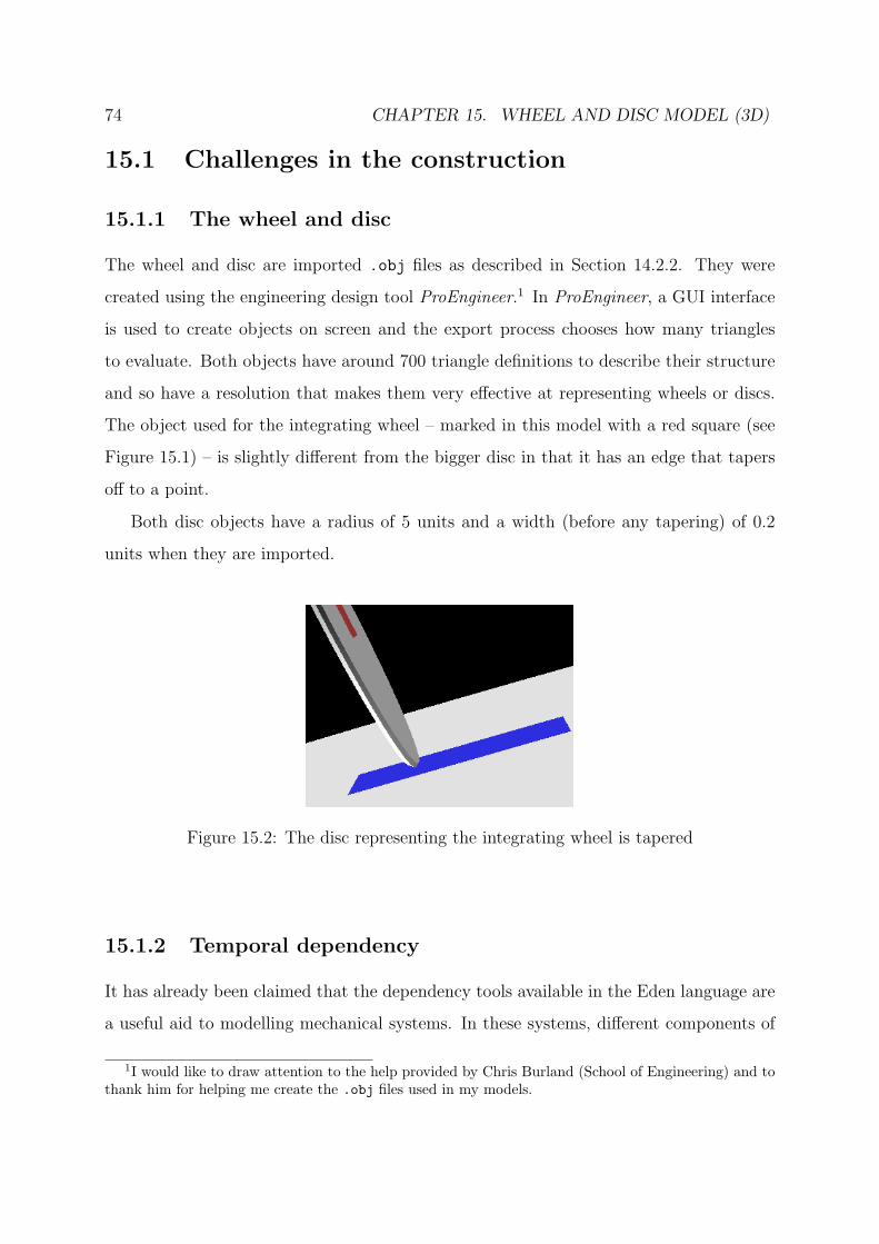
74 CHAPTER 15. WHEEL AND DISC MODEL (3D)

15.1 Challenges in the construction

15.1.1 The wheel and disc

The wheel and disc are imported .obj files as described in Section 14.2.2. They were

created using the engineering design tool ProEngineer.1 In ProEngineer, a GUI interface

is used to create objects on screen and the export process chooses how many triangles

to evaluate. Both objects have around 700 triangle definitions to describe their structure

and so have a resolution that makes them very effective at representing wheels or discs.

The object used for the integrating wheel – marked in this model with a red square (see

Figure 15.1) – is slightly different from the bigger disc in that it has an edge that tapers

off to a point.

Both disc objects have a radius of 5 units and a width (before any tapering) of 0.2

units when they are imported.

Figure 15.2: The disc representing the integrating wheel is tapered

15.1.2 Temporal dependency

It has already been claimed that the dependency tools available in the Eden language are

a useful aid to modelling mechanical systems. In these systems, different components of

1I would like to draw attention to the help provided by Chris Burland (School of Engineering) and tothank him for helping me create the .obj files used in my models.

15.1. CHALLENGES IN THE CONSTRUCTION 75

a mechanism are connected to others by some kind of power transmission like cogs and

shafts. These connections represent a mechanical dependency that can be mapped into

an Eden dependency.

In an initial attempt at this model, such an approach was taken. Mouse motion in the

input frame was linked through dependency to the displacement of the integrating wheel

and the rotation of the large disc.

wheelRatio is drawPanel_mousePos[1];discRotation is drawPanel_mousePos[2];

It then makes sense to define the rotation of the wheel in terms of these. The wheel rolls

over the disc and the amount it rolls depends on the displacement of the integrating wheel

from the centre of the disc. When the wheel is at the centre of the disc (wheelRatio = 0)

the wheel remains stationary and when the wheel is at the edge of the disc (wheelRatio

= 1), it experiences maximum rotation.

wheelRotation is discRotation*wheelRatio;

However, on closer inspection this is not correct at all. The variable wheelRatio

provides us with a value that indicates the gear ratio between the disc and the wheel at

any point. What the above dependency does not take into account is the fact that this

variable can (and most certainly will) vary throughout the runtime of the model. In this

example wheelRotation will be updated each time the wheel is moved and in English is

“the amount the wheel has rotated since the beginning of the planimeter’s runtime, given

that the wheel was positioned in the position corresponding to wheelRatio”.

In order to deliver the required semantics of this variable – where it shows the cumu-

lative rotation over time – a construction was required that could allow the accumulation

of values given by a dependency that requires knowledge of its history.

This code is known as the clock or accumulator procedure in the various models and

is common to all the different types of planimeter.


15.2 Temporal variables

In order to model this relationship it is necessary to represent the varying quantities as

quantities that vary with time.

When integration is introduced to a class of mathematics students; it is common

to talk of changes happening in a small interval (δx), which is then minimised until it

becomes infinitely narrow (dx).

∫f(x)dx

This is represented on the planimeter when x is the movement of the pen along the

track and f(x) is the movement perpendicular to the track.

If the translational movement along the track is seen as a function of time, x = χ(t)

then for a given time interval [t0, t0 + δt] the area under the curve is given by:

(χ(t0 + δt)− χ(t0))(f(χ(t0))

and as this interval is minimised:

∫f(x)dx =

∫f(χ(t))χ(t)dt

The generalisation allows both x and f(x) to be represented by computer variables

that are adjusted after some small amount of time δt.

The clock procedure for a model of a cone planimeter is given in Section 17.3.

15.3 How to run this model

1. Load the script into TkEden

$ /dcs/emp/empublic/bin/tkeden model1.eden

2. Initialise the mouse by moving it into the input frame.

15.4. ISSUES RELATING TO THIS MODEL 77

3. Initialise the time counter by executing the startClock Eden procedure. This starts

the sampling process and allows the mechanism to start working.

startClock();

4. Mouse movements in the input window (the square with axis painted on it) should

now map to the movement of the planimeter’s tracing point.

While tracing, the movement of the disc and wheel are also illustrated in two dimen-

sions on the control panel. The circle with the blue marker illustrates the position of the

disc while the circle with the red marker gives the position of the wheel. The numerical

output inside the latter wheel view gives a numerical output corresponding to the area

traced.

15.4 Issues relating to this model

This model was presented informally to all the other students who were making use of

the empirical modelling tools in their third year projects. In this presentation, it became

clear that there were certain issues in the user interface of the model that needed to be

addressed.

15.4.1 Reseting the model

In the planimeter models, there is a clear need for the user to be able to reset the area

counter or the integrating wheel. This enables a new area to be traced and illustrated on

the counter without having to subtract the start reading. This common task should be

provided with an associated button. Having to do the reset manually by typing in some

code is unacceptable.


15.4.2 Sasami zoom and rotate controls

Because the mouse is used in the input frame, it is necessary to set up the 3D visualisation

of the model before tracing an object. Changing the angle of view or zooming (this is

done in the Sasami window using the different mouse buttons) requires the mouse to have

left the input pane.

15.4.3 Modelling principle or device?

The students who were shown this model found it very difficult to see the wheel and disc

as an area calculator. After some minutes of interaction it was possible to convince them

that the device worked and it was also possible to see the mechanism as a variable gear.

However, the mapping between actions in the input frame and the activity in the Sasami

visualisation proved difficult.

I think this was due to two reasons:

1. It was difficult to see the rotation just using the 3D representation.

2. There was no movement of a ‘pen’ in the simulation and so no clear reason why the

disc was spinning. The mechanism was just floating in mid air without any inputs

or outputs.

For the user acquainted with planimeters, this model is a helpful simulation of the

principle of the variable gear as an integrating mechanism. In this sense, the model

could be seen as a dynamic version of Figure 3.1. What would have suited the audience

unaware of the various planimeter designs would have been to construct the model with

more real-world mapping.

Chapter 16

Wheel and Disc Model (2D)

Earlier it was said that the motivation for the project was that planimeters were a central

component of the differential analyser in which there are a number of planimeters that can

be connected in a number of ways. This model was the start of a more distributed way

of looking at the planimeter models where more than one planimeter could be connected

to an input table.

A ‘problem’ with the basic wheel-and-disc model was that the manipulating of complex

Sasami objects (like discs) in real time is very processor intensive. This model explores

how a two-dimensional (and so less processor intensive) version could be constructed.

16.1 Improvements with respect to the first model

This model addresses some of the issues relating to the 3D version that were raised in

Section 15.4. It implements a distributed model in which the planimeter is on a separate

machine to the input window. In this way one mouse is made available for tracing and

another for controlling the planimeter model.

79


Figure 16.1: A model of a planimeter using DoNaLD

16.2 Starting the model

The model consists of 3 dTkEden1 sessions: the server, planimeter and input table. To

allow one mouse to be dedicated to the tracing and another to the controls the two clients

should be run on separate machines. The server handles communication between the

clients and can be run on either (or another) machine. If having a dedicated mouse isn’t

important then all the clients can be run on the same machine.

Assuming dTkEden is installed at /dcs/emp/empublic/linux-i686/bin/dtkeden

the model is provided with some bash shell scripts to set up the dTkEden sessions.

1. Start the server

$ ./startServer

2. Start the input table

$ ./startInputTable1

1dTkEden is a networked version of TkEden and allows components of a model to be distributedacross a network. It is described more fully in Chapter 18.

16.3. USING THE MODEL 81

3. Sign in to this window with the agent name inputTable1

4. Start the planimeter (may be on a separate machine)

$ ./startPlanimeter1

5. Sign in to this window with the agent name planimeter1

6. Start the planimeter’s clock function by pressing the start button in the clock section

of the control panel.

16.3 Using the model

The model provides 2D viewing of the planimeter as a standard engineering drawing.

The set of axes to the side of the front elevation indicate, with colours, which view is

which. The integrating wheel will spin in proportion to the area being traced if the clock

is running. This clock can be left running, however provision for stopping it has been

provided so that processor power used by dTkEden can be reduced.

Mouse movements in the input table manipulate the position of the wheel on the disc

and the rotation of the disc.

16.3.1 The revolution counter

Initially, the revolution counters show how many revolutions the wheel and disc have

made during the run-time of the model. Rotations of these are also illustrated in the

above and side views of the model. The reset button resets these counters, yet it doesn’t

reset the position of the wheel. This effectively means that the counter shows the number

of rotations since the last press of the reset button. The wheel is not reset to a stationary

position as such an interaction would break the dependency that the wheel only moves by

rolling with the disc. To have such behaviour would be as if the functionality of pressing

the reset button on a car mileage counter were to spin the wheels and return them to the

positions that they occupied when the car was new.


16.4 Evaluation of the model

This model was demonstrated to Ashley Ward and Steve Russ in December. For Ashley,

the model was his first contact with planimeters and it was pleasing how successful the

model was at illustrating the principle.

In this model, instead of the integrating wheel sliding over the disc, the disc moves

under a stationary wheel. This brought it closer in terms of historical accuracy to Wetli’s

design (see Chapter 7).

The reset button is a useful addition since it allows users to trace areas with a counter

starting at zero. Providing revolution counters for both the wheel and the disc was more

misleading than helpful since it wasn’t clear which one was representing the area traced.

It was realised that what was really lacking was a counter that gave the area traced in

units.

The double-workstation set up with the input table is on one machine and the model

on another worked quite well although it was quite difficult for one person to maintain

awareness in both directions. An improved interface might be one where the input table

machine is replaced with an interface device like a graphics tablet. The mouse is a difficult

tool to draw with. The set-up really comes into its own when the system is operating in

a ‘classroom style’ – where an audience is watching a single user interact with the model.

Such a configuration allows the audience to see clearly that the device is performing some

area calculation and they can watch the effect of different interactions more clearly than

if they were the user. This situation is improved further if the audience are encouraged

to give tasks to the operator, or if the task of operating is rotated.

The distributed structure of building a model is very flexible and allows for code re-

use. Future modifications like swapping the software input table for a hardware graphics

tablet could be done quite easily.

Chapter 17

Modelling an Oppikofer Planimeter

It seemed logical that the next model to be constructed should be a cone-and-wheel

planimeter. Because this model contains both a cone and a wheel it seemed appropriate

to use it to describe the modelling process in more detail.

17.1 A starting point

If such an emphasis is to be put on observation, then a logical starting point is to use

a diagram (See Figure 17.1) of what is to be modelled. It is clear from this diagram

that this planimeter has a number of distinct components. The process of modelling will

involve representing each of these as individual components (Section 17.2), assembling

them together, and then linking their interactions (Section 17.3).

17.2 The basic components

17.2.1 The cone

The obj file to be imported for the cone is cone point.obj and contains definitions of

something in the region of 700 triangles.

%sasamiload_obj cone "cone_point.obj"

83

84 CHAPTER 17. MODELLING AN OPPIKOFER PLANIMETER

Figure 17.1: Oppikofer’s planimeter[dM13, p 56]

This imports the polygon and places it at the origin. It is necessary for the uppermost

edge of this cone to be horizontal (see Figure 17.1) so the cone is rotated through 15°.

Its position is also linked through dependency to the variable carriagePos which will

control the position of the cone as it moves along its track from side to side.

%sasamiobject_rot cone_1 15 0 coneRotationobject_pos cone_1 carriagePos 0 0

The reason for the choice of a 15° rotation is because the object file loads an object in

the orientation shown in Figure 17.2. The object needs rotating so that it has the same

orientation as the cone in Figure 17.1.

The variable coneRotation will be a value controlling the rotation (in degrees) of

the cone. Since coneRotation and carriagePos are Eden variables, they need to be

instantiated before the above definitions will take effect.

%edenconeRotation = 0;carriagePos = 0;

17.2.2 The roller

Next it is necessary to add the roller (marked P in Figure 17.1) and to connect it to the

wheel by a shaft. The wheel is another imported object disc.obj

17.2. THE BASIC COMPONENTS 85

````````````````````````````

10 Units5

Unit

s

Figure 17.2: Dimensions of the cone point.obj

%sasamiload_obj roller "disc.obj"

This is also set at 15° and its size adjusted to make the desired shape. The size of this

roller is scaled by an Eden variable roller size and its position defined by three other

variables roller pos x,roller pos y and roller pos z.

%sasamiobject_pos roller_1 roller_pos_x roller_pos_y roller_pos_zobject_rot roller_1 15 0 coneRotationobject_scale roller_1 roller_size roller_size 8*roller_size

17.2.3 The shaft

There will be a shaft connecting the cone and the wheel. Using dependency, it makes

sense to define the position of the roller in terms of the position of the cone and the length

of the shaft. Here is quite a complicated transformation problem that classically would

require the drawing of a diagram and the application of trigonometry. However, because

of the way the Eden variables are used, the model actually becomes our diagram. Since

the point at which the cone is to be connected to the shaft is the origin; we can look at

the problem and start to write down things we know about the distances between points.

%eden


shaft_length=6;roller_pos_x is carriagePos;roller_pos_y is -shaft_length*sin(PI/12);roller_pos_z is shaft_length*cos(PI/12);roller_size = 0.3;

It should be mentioned here that although Sasami uses degrees for its angle measure-

ments, Eden uses radians in its trigonometric functions. So throughout the code, the

equality 15°= π12

is used.

Now we have the roller and cone. Both objects are linked in their rotation and position

by dependency. For example, providing the redefinition coneRotation=20; rotates both

by 20°. The true power of modelling in this way can be seen if the shaft length were

defined to be slightly larger. Figure 17.3 shows how redefining shaft length from 6 to

10 changes the output.

Figure 17.3: Re-Defining the Shaft length

Next a Sasami visualisation of this shaft is required. Represented as a cuboid, the

shaft will be a little longer than shaft length so that it gives the impression of going

through the roller. Reasons for modelling the shaft as a cuboid rather than a cylinder

are twofold; firstly, a cylinder would use something in the order of 700 times the memory,

and secondly, rotation of the more angular cuboid shaft is easier to see.

The shaft used is defined with simple dimensions (see Figure 17.4) and is then stretched

to the correct size (see Figure 17.5). This has enabled me to use the same Eden definitions


10 Units

10U

nits

0.2 Units

Figure 17.4: Dimensions and visualisation of the unscaled shaft

(with different names) elsewhere in the code for other shafts.

%sasamiobject shaft

## Vertices at front of the shaftvertex shaft_a1 -5 5 0vertex shaft_b1 5 5 0vertex shaft_c1 5 -5 0vertex shaft_d1 -5 -5 0## Vertices at rear of the shaftvertex shaft_a2 -5 5 0.2vertex shaft_b2 5 5 0.2vertex shaft_c2 5 -5 0.2vertex shaft_d2 -5 -5 0.2

...

## declaring polygons in terms of vertices## (notice that the order of vertices define which side## of each polygon is solid)poly_geom_vertex shaft_end1 shaft_a1 shaft_b1 shaft_c1 shaft_d1poly_geom_vertex shaft_end2 shaft_d2 shaft_c2 shaft_b2 shaft_a2poly_geom_vertex shaft_sideA shaft_a2 shaft_b2 shaft_b1 shaft_a1poly_geom_vertex shaft_sideB shaft_b2 shaft_c2 shaft_c1 shaft_b1poly_geom_vertex shaft_sideC shaft_c2 shaft_d2 shaft_d1 shaft_c1poly_geom_vertex shaft_sideD shaft_d2 shaft_a2 shaft_a1 shaft_d1

## Attach the Polygons to the Shaft Objectobject_poly shaft shaft_end1 shaft_end2object_poly shaft shaft_sideA shaft_sideB shaft_sideC shaft_sideD


Using this shaft code, the shaft is stretched to the correct size and is placed in the

correct position. To model its physical connection with the cone and the roller, it is

associated through dependency to the coneRotation variable.

%sasamiobject_pos shaft carriagePos 0 0object_scale shaft 0.02 0.02 (shaft_length+8*roller_size*0.3)/0.2object_rot shaft 15 0 coneRotation

Figure 17.5: The shaft object after scaling

17.2.4 The track

The roller needs to roll on a track. This track is defined in Sasami as an angled wedge.

Firstly the dimensions and positions are declared using Eden variables.

%eden## Primary dimensions of tracktrack_width=1;track_height=0.3;track_length=20;

## Secondary dimensions of tracktrack_height_1 is track_height+track_width*sin(PI/12);track_width_1 is track_width*cos(PI/12);


## Track Positiontrack_pos_x = 0;track_pos_y = 0;track_pos_z = 0;

These dimensions are used to create the eight vertices of the track. Polygons are then

created for each side of the track and attached to the track object. Finally, the object is

positioned according to the position variables.

%sasamiobject track

vertex tracka1 0 0 track_width_1vertex trackb1 0 0 0vertex trackc1 0 track_height_1 0vertex trackd1 0 track_height track_width_1

vertex tracka2 -track_length 0 track_width_1vertex trackb2 -track_length 0 0vertex trackc2 -track_length track_height_1 0vertex trackd2 -track_length track_height track_width_1

...

object_pos track track_pos_x track_pos_y track_pos_z

17.2.5 The wheel

The integrating wheel (marked R in Figure 17.1) rolls on the uppermost surface of the

cone as the cone rotates. Much like the cone, the wheel also has an angular displacement:

%edenwheelRotation = 0;

The wheel is an imported object with diameter 10 units.

...%sasamiload_obj wheel "disc_taper.obj"object_pos wheel_1 wheel_pos_x wheel_pos_y wheel_pos_zobject_rot wheel_1 0 0 wheelRotationobject_scale wheel_1 wheel_size wheel_size wheel_size...


This wheel is allowed to slide along the surface of the cone as the function being

integrated varies.

The wheel’s position is represented by the variable wheelPos which ranges over the

interval [0,1].

%edenwheelPos = 0;

If wheelPos = 0 then the wheel is at the point of the cone and if wheelPos = 1 the

wheel is at the base of the cone. The variable that defines the z-coordinate of the wheel

is linked to this variable through dependency.

%edenwheel_pos_z is 2.5*sin(PI/12)-wheel_width-9.85*(1-wheelPos);

In this code the numerical constants refer to the dimensions of the cone.

17.2.6 The pen shaft & carriage

As well as the defined components, the actual model also includes a carriage and a shaft

that links the wheel to a pen. These can be seen Figure 17.1, the carriage being component

A and the shaft being component T.

Figure 17.6 shows all these components assembled together.

17.3 Dynamic rolling

So far, the modelling has been static, that is to say the components have been placed in

various places around the model. The rotating components have been defined in terms of

an angular displacement from some starting position.

In order to get the planimeter to perform integration, the model needs to become more

dynamic. It is necessary, for example, to model a small change in coneRotation and to

see this change as the cause of a proportional change in wheelRotation.

A variable representing the rotation of the cone due to the roller rolling over the track

is given by coneSpindleRotation. This is directly linked through dependency to the

roller’s position.

17.3. DYNAMIC ROLLING 91

Figure 17.6: The assembled planimeter

coneSpindleRotation is -360*carriagePos/(2.5*2*PI);

The actual rotation displayed on the screen is given by coneRotation which is syn-

chronised with coneSpindleRotation after every time period. Hence, the rotation of the

cone in the last δt time units is given by the difference between coneSpindleRotation

and coneRotation. Since this is the angular displacement of the cone during one time

unit, it is also the average speed of the cone in that time unit.

An Eden procedure clock() is used to model this regular work. The change in rotation

is calculated, then the rotations are synchronised and the final work is to place a call to

clock() back onto the stack. This (todo) statement ensures that the next clock cycle

happens soon. This is vague enough for our purposes, the length of the time interval δt is

irrelevant and can even vary from clock cycle to clock cycle as long as it stays sufficiently

small.

Clearly, there needs to be activity taking place during each clock cycle that controls

the changes in the wheel’s position. We recall the use of the variable wheelPos in Section

17.2.5. If wheelPos is zero then the wheel is at the pointed end of the cone and doesn’t

rotate at all. However, as wheelPos grows, the wheel rolls proportionally more for a given


rotation of the cone. Hence, some code is added to clock() to calculate the change in

the wheel’s angular displacement, and to accumulate this rotation.

Also added to this procedure is a boolean condition clockGoing which allows graceful

termination of the clock without the use of the interrupt button in TkEden.

proc clock {## Cone speed is the change in angular displacement in the last time unitconeSpeed = coneSpindleRotation-coneRotation; ## rads / time## coneRotation is accumulatedconeRotation = coneRotation+coneSpeed;## wheelSpeed is defined in terms of the coneSpeed## And is the change in angular displacement during the last time unitwheelSpeed = -(wheelPos*coneSpeed);## wheelRotation is accumulatedwheelRotation = wheelRotation+wheelSpeed;

## Re-run this procedure soon if not stopped.if (clockGoing == 1) {

todo("clock();");}

};

17.4 Input

The last addition is to add an input window and to link mouse movements in this window

to the movement of the tracing pen.

%edenwheelPos is drawPanel_mousePos[2];carriagePos is -8+16*drawPanel_mousePos[1];

17.5 Running the model

The model can be loaded by executing the Run.e Eden script from the model directory.

$ tkeden Run.e

17.5. RUNNING THE MODEL 93

To enable the rolling, the clock needs to be started.

%edenclock();

A screen shot of the final model is given in Figure 17.7. Movement in the window

labelled “screen” will cause movement of the 3D representation in the window labelled

“sasami”.

Figure 17.7: The final model

Chapter 18

Distributed Framework

Separating the different elements of the model was so successful in the 2D model (see

Section 16) I decided that it should be constructed in a more general context. Planimeter

models could then be constructed for this framework that make use of a common input

table. There would also be the facility for one input table to drive a number of planimeter

models and so allow comparisons of the different mechanisms.

18.1 dTkEden

dTkEden stands for distributed TkEden and provides networkable support for models.

A dTkEden window is identified as an agent and has a defined way of interacting with

the rest of the model. An agent has a list of global variables that it monitors, known as

oracles, and a list of global variables that it has permission to update, known as handles.

One dTkEden session runs in server mode and is responsible for receiving updated state

from agents with handles and ensuring that agents with oracles are delivered information

about relevant state change.

18.2 Structure of the framework

The planimeter framework is a fairly straight-forward dTkEden set up because there are

only two types of agents – input table and planimeter. The communication model is

95

96 CHAPTER 18. DISTRIBUTED FRAMEWORK

simple since input table only has handles on variables and planimeter only has oracles.

� The input table provides the user with an interface for moving the pen and manipu-

lates global state (on the server) when the position of the pen changes (or the scales

used on the table are modified).

� The planimeter model responds to the motion of the pen (sent to it by the server)

and provides the user with a visualisation.

Server

PlanimeterInput Table

Figure 18.1: Communication in the framework is one-way

The background to this framework was the work done in the 2D model (See Chapter

16) where there was provision for two input tables and two planimeters. I found that

the most useful configuration was one input table with two planimeters connected to it.

For this reason, this version and all subsequent versions of the framework were developed

with one input table. This modification made it it easier to implement the scaling factors

that allow the same input table to represent different scales of quantity.

18.3 A generic input table

The main benefit of the framework is to allow one input interface to be used on all the

planimeters. Because the input table can be re-used, it was justifiable to allocate some

18.4. MODIFICATION OF THE CONE PLANIMETER 97

time to developing it further. In the previous models, dividing the user’s attention across

two monitors was identified as being a problem. Actions on the input table were causing

the planimeter to move when there should been feedback in the input table. The improved

input table provides some feedback by having an on-screen cursor showing the position

of the tracing pointer.

It was also noticed that it was often helpful for users to investigate the model while

someone else was drawing for them. The new input table provides support for automatic

drawing so that the computer can automatically draw simple shapes like the unit square.

To ease tracing, grid lines were added to the input table.

Figure 18.2: The new input table

18.4 Modification of the cone planimeter

The cone planimeter described in the last chapter was re-written for this framework so

that it used the standard variable names for the interface. This lead to the development


of a standard control panel that could also be re-used in other planimeter models.

Figure 18.3: The Oppikofer model modified for the framework

18.5 A generic control panel

The control panel was intended to bring together the best parts of the interfaces so far.

They are based on those of the 2D planimeter model, and include controls for the clock,

the reset button and a sideways view of the integrating wheel.

18.5.1 Clock control

There had to be a clock control and in previous designs this had been provided by two

buttons start and stop. This had bad HCI considerations since a user could press either

button at any time. In the new design there is one button that switches its function

depending on the status of the clock.

18.6. EXTENDING THE FRAMEWORK 99

18.5.2 Revolution/area counters

The end-view of the integrating wheel which was a successful component of the 2D model

continues to help the user monitor the rotation of the wheel.

The representation of the area has however quite changed. The revolution counter for

the disc (that was of no real use) has been removed to reduce confusion. As before, the

reset button resets the numerical counters but not the wheel’s physical position.

The new addition to the controls is the second counter that gives the area traced in

units. The size of an area unit is configurable by the user by pressing the calibrate button.

Pressing this button is as if to say “the area represented by the current rotation of the

wheel (since the last zero point) is equal to the unit square”.

Figure 18.4: The new control panel

18.6 Extending the framework

An obvious application of this framework would be to allow the construction of a differ-

ential analyser model. For this to be possible, three extensions or adaptions would need

to be made.

1. The provision for numerous input tables would have to be re-introduced. This is a

fairly trivial addition.

2. An output table that was capable of plotting a function would need to be modelled.


3. The planimeter models would have to be developed so that they can output data.

This would require more complex models.

For more about these and other possible extensions to the project see Section 21.5.

Chapter 19

Modelling a Wetli Planimeter

The second planimeter to be built in the framework was of the Wetli-Starke type. In this

sense this model is very much a refined version of the wheel-and-disc planimeter models

that were referred to earlier (Chapters 15 and 16). One criticism of these earlier planime-

ters was that they just showed the wheel and disc rotating in the abstract without the

context of their guiding rails, carriages or shafts. This model tries to address those issues

by merging the success of the cone planimeter model with the original work undertaken.

Like the cone model, this planimeter was designed as a 3D model from scratch. It

makes use of the Eden function macro()1 that allows common code to be reproduced by

variable substitution.2 This function was used to generate all the cuboids in the model

and makes the code much easier to understand.

19.1 Using the macro function

To generate a object in Sasami; all vertices and surfaces need to be defined separately.

A section of Sasami script to define a cube might therefore be the declarations of the 8

vertices.

1macro() is missing from the Eden Handbook and really should not be. It is a very useful toolparticularly for Sasami when huge amounts of code have to be reproduced to copy something simple likea cube.

2macro() reads a character string and replaces occurrences of ?1,?2,...etc. with character strings thathave been passed to it.

101

102 CHAPTER 19. MODELLING A WETLI PLANIMETER

...vertex cube_a 0 0 0vertex cube_b 3 0 0vertex cube_c 3 2 0vertex cube_d 0 2 0

vertex cube_aa 0 0 3vertex cube_bb 3 0 3vertex cube_cc 3 3 3vertex cube_dd 0 3 3...

macro() can be used to generate this code.

%eden ## We’re in edencubeMacro=" ## The macro is an eden variable *containing*

## sasami code%sasami

vertex ?1_a 0 0 0vertex ?1_b ?2 0 0vertex ?1_c ?2 ?2 0vertex ?1_d 0 ?2 0

vertex ?1_aa 0 0 ?2vertex ?1_bb ?2 0 ?2vertex ?1_cc ?2 ?2 ?2vertex ?1_dd 0 ?2 ?2

";execute(macro(cubeMacro,"cube","3")); ## execute this code

Where "cube" replaced the substitution variable "?1" and "3" was substituted for

"?2".

A whole cube has been written as a macro and is provided as an example model (see

Appendix B).

19.2 Constructing the model

This model took a slightly different approach. Starting from a rough sketch, key dimen-

sions were represented by Eden variables. From there other dimensions were defined with

dependency allowing cuboids defined by macros to be sized correctly and placed at appro-

priate places. This provided the model with a great flexibility of interaction, one example

of which is shown below.

19.3. MANIPULATING THE MODEL 103

Figure 19.1: A model of a Wetli planimeter

19.3 Manipulating the model

Being designed around dimensions allows some interesting modifications to be made to

the model at run-time. For example, we could perhaps investigate what would happen if

the track were extended.

## Set the dimension trackLength to 5 times it’s previous value%edentrackLength=trackLength*5;

Changing a dimension like this causes a number of vertices and polygons to be re-

defined as the track is stretched (see Figure 19.2).

19.4 Running the model

This model is included in the framework directory as planimeter1.

104 CHAPTER 19. MODELLING A WETLI PLANIMETER

Figure 19.2: The model with a stretched track

Chapter 20

Modelling a Amsler Planimeter

The model of an Amsler planimeter was a late addition to the models produced and was

actually written to assist my understanding of their mechanism. In this sense, the model

is a superb advocate for the empirical modelling tools being a way of “thinking with

computers”. The diagram is in 2D (in DoNaLD) which was found to be quite sufficient to

illustrate this type of mechanism. Another motivation for the model was ‘The Planimeter

Applet’ (described Section 13.1) although the model is not as complex as the applet –

which uses 1000 lines more code. However, most of the interaction provided by the applet

could be incorporated into the Eden model fairly easily.

The model illustrates the two arms of the Amsler planimeter as two lines between

three dots. One of these dots represents the tracing point. An end-on visualisation of

the wheel is provided to show the rotation and a reset button to reset the counter. In an

actual polar planimeter, the wheel is mounted at some point along the arm between the

pivot point and the tracing pen.

Unlike the reset button of the earlier wheel-and-disc model (Section 16.4), the reset

button on the Amsler model does rotate the wheel to an initial starting point. This is

how the planimeters were actually operated. The planimeter was lifted off its surface and

the wheel was moved to the zero point.1

1check reference in [Hen94]

105

106 CHAPTER 20. MODELLING A AMSLER PLANIMETER

Figure 20.1: The Amsler planimeter in 2D

20.1 How to run this model

This model requires no setting up or networking. It is just loaded into TkEden and starts

working.

$ /dcs/emp/empublic/bin/tkeden amslerModel.eden

The reset button will reset the area counter. Once it has been clicked (and is therefore

in focus) it is sensitive to key actions. This provides the means – by hitting any key – to

reset the area counter while tracing.

Chapter 21

Conclusion

The original specification of the project is included in Appendix A. The project was high-

lighted as having three main components; history, modelling and presenting the history.

21.1 History

At the beginning of the project I set myself three objectives for the historical research.

I wanted to find out about the different people involved, how their work related to each

other and what their motivation was.1 Looking at the inventors individually has confirmed

that many people did conceive of the idea independently. In terms of motivation, it was

the need to measure land area that created the need for planimeters to be invented. It

has been interesting to look at how many of the early planimeters were brought together

at the Great Exhibition. It would be interesting to look at planimeters displayed at

other European exhibitions of the same period. It is fascinating that Sang’s work was

so independent of the European work and one day I would like to be able to answer the

question of how much Maxwell or Thomson’s innovation was isolated from Europe.

1See Section A.1

107

108 CHAPTER 21. CONCLUSION

21.2 Modelling

Producing models of historical devices is a great challenge. There is a tension between

historical accuracy and the illustration of principle. In my models the emphasis has

usually been on providing users with a tool to understand the principle of a planimeter

rather than just being a digital exhibit.

The project has been successful in demonstrating that an analogue device can be

modelled on a digital platform. Using tools that support dependency was definitely the

correct choice, I am very pleased that most of the models have analogue principles encoded

in the deepest elements of their behaviour. In this way the models really are analogue in

‘thought and word and deed’.

21.3 Illustrating history

The ‘presentation’ section of the project has received the least treatment. It was hoped

that “some kind of hypermedia”2 would be produced. Unfortunately, this area of work

did not fit into the time constraints of the project.

My planimeter models have had a great deal of exposure to a variety of audiences. As

well as the project presentation, the models have been used on an open day and shown to

interested academics. Their value as a teaching aid should not be underestimated. When

exhibited at a department open day, the models were being used by people who had never

even heard of planimeters before.

21.4 Project management

21.4.1 Timetable

Section A.6 shows the original timetable for the planned work. The flow of work outlined

here was adhered to without much alteration. Forcing myself to produce extra documen-

2See Section A.2

21.5. FURTHER WORK 109

tation worked well – especially the ‘inventor report’3 produced at the end of term 1.

I found that tasks based around writing tended to require more hours than expected

whereas – unusually for Computer Science – the coding actually took less. The research

element of the project consumed as much time as was allocated although I was extremely

pleased with the results that have been achieved. Preparation for the presentation ran to

schedule.

21.4.2 Writing

The discipline of producing structured writing early on in the project provided some

basic content for starting the report-writing phase. Using LATEX for all documentation

(including the presentation slides) enabled me to develop proficiency with both LATEX and

BibTEX and to have the confidence to use these tools in my report.

21.4.3 Website

All finished documentation was published on my project web pages. This helped me visi-

bly track the project’s progress and provided something for interested parties to explore.

Screenshots from my models were also added to the site giving a complete picture of the

work going on.

21.5 Further work

21.5.1 Further integration of history and models

As they stand, the models need some kind of background explanation. Further work

should be done with the models to allow them to be presented alongside some form of

hypertext. Earlier it was suggested that a browser ‘plug-in’ version of TkEden could be

developed.

3See Section A.4.

110 CHAPTER 21. CONCLUSION

21.5.2 Modelling the differential analyser

The background to investigating the history of the planimeter was the use of wheel-and-

disc integrators in the differential analyser. A logical extension to the project would be

to connect planimeters together and model a differential analyser.

21.5.3 The development of the polar planimeter

The widely manufactured polar planimeter was only touched on by this project. Further

research should be done to access the originality of the various developments relating to

the original work of Amsler. Models of rolling planimeters would be an interesting goal

to work towards.

Appendix A

Project Specification

Illustrating the History of the PlanimeterCharles Care

17th October 2003

A.1 Problem

“The most common form of mathematical instrument available in thenineteenth century was the planimeter.”1

An analogue device that can perform mathematical integration, the planimeter wasfirstly invented in Bavaria in 1814.2 Throughout the 19th century it was developed ina variety of ways, recieving many of its improvments from famous scientific names suchLord Kelvin and James Maxwell.3 Later it would become a central component of famousmachines like Kelvin’s Harmonic Analyser and the Differential Analysers of the early 20th

century.4

The purpose of the project is to trace the history of this significant, but often forgot-ten device; and to illustrate and present the story of its development with a number ofcomputer-based graphical models. To this end, three main components of the project canbe identified.

� History – Particulary of interest are the people involved, how their work related toeach other, and what the motivation for their work was.

� Modelling – To produce some simulation of the devices researched.

� Presentation – It is hoped that the research and the models can be linked togetherto provide an accessible way of exploring the history.

1(Mary Croarken: Early Scientific Computing in Britain. Oxford 1990.)2(William Aspray: Computing before Computers. Iowa University Press 1990)3(Simon H Lavington: Early British Computers. Manchester University Press 1980)4(William Aspray: Computing before Computers.)

111

112 APPENDIX A. PROJECT SPECIFICATION

A.2 Objectives

The project will involve work in the following areas:

1. Research into the history of the planimeter.

� Learning how to find and use historical sources.

� Learning how to write-up and cite historicial research.

� Representing the history in an accessible way, perhaps as some form of hyper-media.

2. How to model an analogue device.

� Evaluation of potential modelling methods/tools.

� Producing flexible models that illustrate the development history of the planime-ter.

A.3 Methods

It is planned that research will continue throughout the project in parallel with the mod-elling process. A number of milestones are defined in the project timetable which willsynchronise these two separate areas of work from time to time.

Regular project reports will be produced, to keep track of current progress.The project can be split into a number of tasks. These are laid out in a Gantt Chart

that appears as an appendix to this document.

A.3.1 Preparation for Modelling

The following tasks are identified as being necessary before work on the final models begin.

� Learning Basic Eden & Associated Tools – It is planned to spend a few weeks work-ing on some example code and understanding the Emperical Modelling Paradigm.

� Java 3D – Some time will be spent learning the basics of Java 3D.

� JaM API – Some time will be spent becoming more familiar with this way of usingdependencies in a Java context.

� Language Evaluation – Once a working knowledge of both the Eden-based toolsand the JaM framework has been acquired, a basic model of the planimeter willbe attempted in both languages. Although these models may not reach a finishedstate, it should be clear after some initial work which environment will offer thebest trade-off between presentational quality and flexibility of design. The findingsof this evaluation will be presented in a report.

A.3. METHODS 113

A.3.2 The Modelling Process

This will begin in week 9 and will draw on the research undertaken in term 1. It is possiblethat further research might adjust the way the model is structured and any new materialwill be merged at the begining of term 2.

Models will be built in the language proposed by the preparatory work.

A.3.3 The Research Process

The research process can be broken down into two main sections, preliminary researchand the preparation of some research reports. The preliminary work will be completedwithin a few weeks and the two initial documents a few weeks later. Once completed,these two reports will form a basis to decide which areas the project should focus on.

Preliminaries

Some work has already been undertaken during the summer to locate some basic sourcesfor the historical element of the project. Brief notes on these sources can be found in thefollowing project documents.

� project-notes-001






Research Documents

Two documents will be produced during the first term to summarise the research under-taken. These reports will form the basis for deciding what the research focus should befor the rest of the project.

1. A summary of the inventors.

2. A summary of the types of planimeter.

114 APPENDIX A. PROJECT SPECIFICATION

A.4 Timetabled Milestones

1. Term 1 Week 5: Summary of Inventors.

2. Term 1 Week 7: Modelling Language Report

3. Term 1 Week 8: Summary of Devices.

4. Term 1 Week 10: End of Term Progress Report

A.5 Resources

The first part of the Project is mainly research based and so the use of library facilities(both internal and external) will be employed. For the modelling it is planned that thebulk of work should be undertaken locally on the dcs machines using either tkeden or theJava JaM API.

It is possible that some work will be undertaken remotely. The intention is that anyremote work will be synchronised and if necessary merged with the data on dcs serversas often as practical.

The project is intended to be dependent on campus-based computing so that anypersonal facilities used are non-essential.

A.5.1 Report Writing Tools Identified

� Basic Unix

� LATEX

� Perl

A.5.2 Modelling Tools Identified

� Java SDK

� TkEden – Warwick Empirical Modelling

� DoNaLD – Warwick Empirical Modelling

� Sasami – Warwick Empirical Modelling

� JaM – Warwick Empirical Modelling

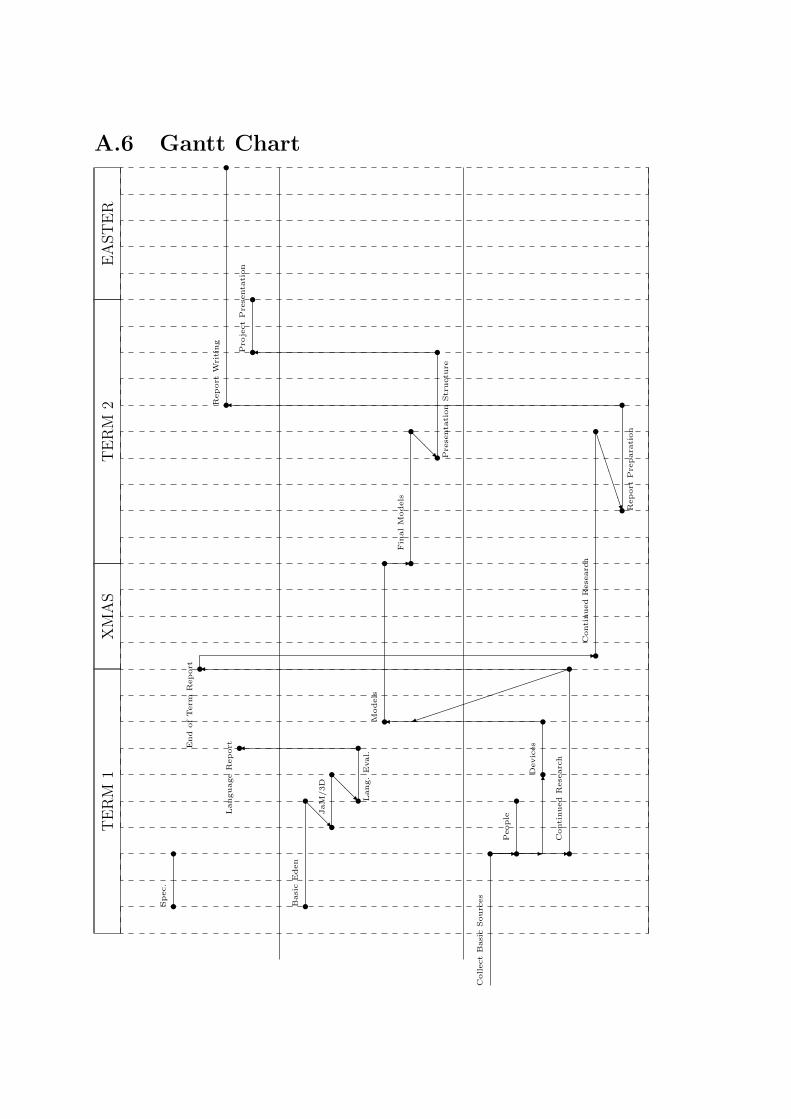
A.6 Gantt Chart

TE

RM

1X

MA

ST

ER

M2

EA

ST

ER

Spec. s

s

End

ofTerm

Report s -

Language

Report s

Report

Wri

ting

s

s

Pro

ject

Pre

senta

tion

ss

Basi

cEden

s

s@@R

JaM

/3D

ss@@R L

ang.

Eval.

ss�

Models s

s -FinalM

odels

s

s@@R P

rese

nta

tion

Str

uctu

re

s

s�

Collect

Basi

cSourc

es

s - -

6

-

People

ss D

evic

es

ss�

Conti

nued

Rese

arc

h

s

s� ��)

Conti

nued

Rese

arc

h

s

sBBBBBBN R

eport

Pre

para

tion

s

s�

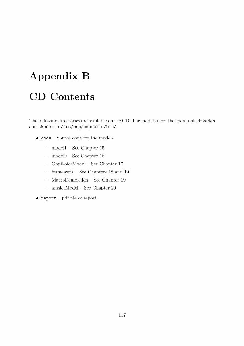
Appendix B

CD Contents

The following directories are available on the CD. The models need the eden tools dtkedenand tkeden in /dcs/emp/empublic/bin/.

� code – Source code for the models

– model1 – See Chapter 15

– model2 – See Chapter 16

– OppikoferModel – See Chapter 17

– framework – See Chapters 18 and 19

– MacroDemo.eden – See Chapter 19

– amslerModel – See Chapter 20

� report – pdf file of report.

117

Bibliography

[Anoa] Diagram of Clair’s planimeter from the Science Museum.

[Anob] Wetli-starke planimeter. Science Museum (Exhibit Label).

[Anoc] Wetli-starke planimeter (new version). Science Museum (Exhibit Label).

[Asp90] William Aspray, editor. Computing before Computers. Iowa State UniversityPress, 1990.

[Bax29a] D. Baxendall. Calculating machines. Encyclopaedia Britannica 14th Edition,4:548–53, 1929.

[Bax29b] D. Baxendall. Mathematical instruments. Encyclopaedia Britannica 14th Edi-tion, 15:69–72, 1929.

[Bro90] Allan G. Bromley. Analog Computing Devices, pages 159–199. In Aspray[Asp90], 1990.

[Car00] B. Carter. Sasami project report. Third Year Project, Dept. Computer Science,Warwick University, 2000.

[Cas51] F Castle. Practical Mathematics Stage II. Macmillan and Co, London, 1951.

[CG82] Lewis Campbell and William Garnett. The Life of James Clerk Maxwell.Macmillan and Co., 1882.

[CKA96] Martin Campbell-Kelly and William Aspray. Computer, a History of the In-formation Machine. BasicBooks, New York, 1996.

[Cli95] Gloria Clifton. Directory of British Scientific Instrument Makers, 1550-1851.Zwemmer, London, 1995.

[Cly93] A. Ben Clymer. The mechanical analog computers of Hannibal Ford andWilliam Newell. IEEE Annals of Computing, 15(2), 1993.

[Cra47] Crank. The Differential Analyser. Longmans Green & Co., London, 1947.

[Cra97] A D D Craik. Edward Sang. In www [www04a]. Available at http://www-history.mcs.st-andrews.ac.uk/history/.

119

[Cro90] Mary Croarken. Early Scientific Computing in Britain. Clarendon, Oxford,1990.

[CU14] G.A. Carse and J. Urquhart. Planimeters, pages 190–206. In Horsburgh[Hor14], 1914. Reprinted 1982, Charles Babbage Institute Reprint Series forthe History of Computing, Tomash Publishers, Los Angeles.

[dM13] Henri de Morin. Les Appareils D’Integration. L’Ecole Polytechnique, Paris,1913. Avaliable on-line from Cornell University historic manuscript collectionhttp://historical.library.cornell.edu.

[Dyc92] Walther Dyck. Katalog Mathematischer und Mathematisch-PhysickalischerModelle, Apparate und Instrumente. Munchen, 1892.

[Fif61a] Stanley Fifer. Analogue Computation, Vol I. McGraw–Hill, New York, 1961.

[Fif61b] Stanley Fifer. Analogue Computation, Vol III. McGraw–Hill, New York, 1961.

[Fis95] Joachim Fischer. Instrumente zur Mechanischen Integration, Ein Zwischen-bericht. In 25 Jahre Lehrstuhl fur Geschichte der exakten Wissenschaften undder Technik an der Technischen Universitat Berlin 1969-1994, 1995.

[Fis02] Joachim Fischer. Instrumente zur Mechanischen Integration II, Ein (weiterer)Zwischenbericht, 2002. Longer version of what was published.

[Fis04] Joachim Fischer. Private correspondence, 2004.

[GE51] Great Exhibition of Works of Industry of all Nations, 1851 : official descrip-tive and illustrated catalogue. Spicer Bros. with W. Clowes and Sons, 1851.Published with the authority of the Royal Commission.

[GE52] Exhibition of the Works of Industry of all Nations, 1851 : reports by the ju-ries on the subjects in the thirty classes into which the exhibition was divided.Clowes, London, 1852.

[GL70] G. Green and G. Lloyd, editors. Kelvin’s Instruments and the Kelvin Museum.1970.

[Har47] Douglas R. Hartree. Calculating Machines: Recent and Prospective Develop-ments and their Impact on Mathematical Physics. Cambridge University Press,1947. Reprinted 1984, Charles Babbage Institute Reprint Series for the Historyof Computing, Tomash Publishers, Los Angeles.

[Har49] Douglas R. Hartree. Calculating Instruments and Machines. Illinois Press,Urbana, 1949. Reprinted 1984, Charles Babbage Institute Reprint Series forthe History of Computing, Tomash Publishers, Los Angeles.

[Har90] P.M. Harman, editor. The Scientific Letters and Papers of James ClerkMaxwell, volume I (1846-1862). Cambridge University Press, 1990.

[Har95] P.M. Harman, editor. The Scientific Letters and Papers of James ClerkMaxwell, volume II (1862-1873). Cambridge University Press, 1995.

[Har02] P.M. Harman, editor. The Scientific Letters and Papers of James ClerkMaxwell, volume III (1874-1879). Cambridge University Press, 2002.

[Hen94] O. Henrici. Report on planimeters. In Report of the Sixty-forth Meeting of theBritish Association for the Advancement of Science, pages 496–523, 1894.

[Hor14] E. M. Horsburgh, editor. Handbook of the Napier Tercentenary Celebrations,or Modern Instruments and Methods of Calculation. Bell, London, 1914.Reprinted 1982, Charles Babbage Institute Reprint Series for the History ofComputing, Tomash Publishers, Los Angeles.

[Kni51] C[harles] Knight, editor. Knight’s Cyclopaedia of the Industry of All Nations.London, 1851.

[Kni01] A. Knights. Modelling a physical environment with empirical modelling. ThirdYear Project, Dept. Computer Science, Warwick University, 2001.

[Lav80] S. Lavington. Early British Computers. Manchester University Press, Manch-ester, 1980.

[Lei04] Larry Leinweber. The Planimeter Applet, 2004. Available athttp://www.leinweb.com/snackbar/planimtr/planimtr.htm.

[Max55a] James Clerk Maxwell. Description of a New Form of Platometer an Instrumentfor Measuring the Areas of Plane Figures, pages 230–237. In Niven [Niv90],1855.

[Max55b] James Clerk Maxwell. Description of a New Form of Platometer an Instrumentfor Measuring the Areas of Plane Figures, pages 275–279. Volume I (1846-1862)of Harman [Har90], 1855. Draft of a paper read to the Royal Scottish Societyof Arts.

[Max55c] James Clerk Maxwell. From a Letter to Cecil James Monro, pages 280–281.Volume I (1846-1862) of Harman [Har90], 1855.

[Max55d] James Clerk Maxwell. From a Letter to John Clerk Maxwell, page 325. VolumeI (1846-1862) of Harman [Har90], 1855. 24th September 1855.

[Max55e] James Clerk Maxwell. From a Letter to John Clerk Maxwell, page 325. VolumeI (1846-1862) of Harman [Har90], 1855. 12th November 1855.

[Max79] James Clerk Maxwell. Letter to James Thomson (with reply), pages 829–230.Volume III (1874-1879) of Harman [Har02], 1879.

[Mor55] Authur Morin. De Mecanique et donnees D’Exprience. Librairie de l’Hachetteet Cie, Paris, 1855.

[Nas90] S[tephen] G. Nash, editor. A History of Scientific Computing. ACM Press,New York, 1990.

[Niv90] W.D. Niven, editor. The Scientific Papers of James Clerk Maxwell. CambridgeUniversity Press, 1890.

[Oca28] Maurice Ocagne. Le Calcul Simplifie. 1928. Translated 1986, Charles BabbageInstitute Reprint Series for the History of Computing, Tomash Publishers, LosAngeles.

[OR96a] J J O’Connor and E F Robertson. Arthur Jules Morin. In www [www04a].Available at http://www-history.mcs.st-andrews.ac.uk/history/.

[OR96b] J J O’Connor and E F Robertson. Jean Victor Poncelet. In www [www04a].Available at http://www-history.mcs.st-andrews.ac.uk/history/.

[RS76] Transactions of the Royal Society of London, volume 24. 1876.

[RSS52] RSSA. Report on the platometer. In Transactions of the Royal Scottish Societyof Arts vol 4, pages 126–129, 1852.

[San52] John Sang. Description of a platometer. In Transactions of the Royal ScottishSociety of Arts vol 4, 1852.

[Sch93] Hyman A. Schwartz. The Willis planimeter. Rittenhouse, the Journal of theAmerican Scientific Instrument Enterprise, 7(2):60–63, 1993.

[Sma01] J[ames] S. Small. The Analogue Alternative. Routledge, London, 2001.

[Svo48] Antonın Svoboda. Computing Mechanisms and Linkages. McGraw-Hill, 1948.

[Tai79] Sir W. Thomson & P. G. Tait. Treatise on Natural Philosophy, volume I, partI. Cambridge University Press, 1879.

[Tho76a] James Thomson. An integrating machine having a new kinematic principle.In RS [RS76].

[Tho76b] Sir W. Thomson. The integral of the product of two given functions. In RS[RS76].

[Tho76c] Sir W. Thomson. Mechanical integration of linear differential equations of thesecond order with variable coefficients. In RS [RS76].

[Tho76d] Sir W. Thomson. Mechanical integration of the general linear differential equa-tions of any order with variable coefficients. In RS [RS76].

[Tho10] S[ilvanus] P. Thompson. The Life of William Thomson, Baron Kelvin of Largs,volume II. Macmillan, 1910.

123

[Vol00] H H Vollrath. Aus der geschichte der planimeter. 2000. Available athttp://www.mathematik.uni-wuerzburg.de/History/ausstell/planimet/geschichte.html.

[Woo00] J. Woodforth. Interactive vrml front-end to dtkeden. Third Year Project,Dept. Computer Science, Warwick University, 2000.

[www00a] Aus der geschichte der planimeter, 2000. Available athttp://www.sciencemuseum.org.uk/collections/treasures/manch2.asp.

[www00b] Gebruder HAFF, 2000. Available at http://www.haff.de.

[www00c] Inventor james watt, 2000. Available athttp://www.ideafinder.com/history/inventors/watt.htm.

[www00d] Tamaya technics, 2000. Available at http://www.tamaya-technics.com/index-e.htm.

[www04a] History of Mathematics Website, St Andrews University, 2004. Available athttp://www-history.mcs.st-andrews.ac.uk/history/.

[www04b] Words of Lord Kelvin, 2004. Quoted from Baltimore Lectures John HopkinsUniversity 1904, p.187.Available at http://zapatopi.net/kelvin/quotes.html.