1

LABORatorio R. Revelli

Centre for Employment Studies

What does the ECHP tell us about labour status misperception:

a journey in less known regions of labour discomfort

by

Matteo Richiardi

Working Papers Series No. 10

Collegio "Carlo Alberto" via Real Collegio, 30 - 10024 Moncalieri (TO) Tel. +39 011.640.26.59/26.60 - Fax +39.011.647.96.43 – www.labor-torino.it - labor@labor-torino.it

LABOR is an independent research centre within Coripe Piemonte

2

LABORatorio R. Revelli

Centre for Employment Studies

What does the ECHP tell us about labour status misperception:

a journey in less known regions of labour discomfort

by

Matteo Richiardi*

February 2002

Abstract This study uses ECHP data to give insights on the characteristics of people whose self-assessment of labour status differs from that of the LFS. We do some ‘labour accounting’, in order to clarify the connection between individual perception and LFS categorisation. We find that discrepancies are frequent, regional differences are extremely relevant in explaining them and thus traditional statistics may be strongly biased in capturing people’s well being in relationship with their labour status. We concentrate then on the most relevant perception errors, above all those connected with searching behaviour, in order to explain their determinants. What emerges is a map of social characteristics explaining discouragement and passive behaviour. Such an attitude is (paradoxically) reinforced by assistance from the state itself, such that it becomes – to a certain extent – ‘institutionalised’. Finally, we show that our understanding of the relationship between misclassification and individual characteristics leads to a reduction in the measurement error to be dealt with in transition flows analysis. *

* LABORatorio Riccardo Revelli

3

Introduction The unemployment rate is probably the most used indicator of labour market performance and of the well-being of an economy as a whole, but in practice it is really difficult to categorise people as either in or out of the labour force or as employed/unemployed. To facilitate comparisons of labour market performance between countries and over time, the International Labour Organisation (ILO) has set forth guidelines for classifying individuals into different labour market states1. In general, these guidelines have been followed by most statistical bureaus in preparing their labour force surveys; moreover, to achieve the goal of international comparability standardised statistics are compiled2. According to ILO definitions, a person is considered unemployed if three requirements are satisfied: 1) the person is not working; 2) the person is currently available for work; 3) the person is actively seeking for a job. While most labour economists agree that the first two criteria are quite straightforward, this is not the case for the third one, which defines the boundaries between unemployed, discouraged and inactive workers. Many studies have shown that the availability and willingness to work might be sufficient to categorise a worker as belonging to the labour force, especially in less developed countries, where search is usually more costly and where searching behaviour, given the importance of the rural sector and of family links, might be less meaningful (Byrne and Strobl, 2001). The issue has also been analysed in some developed countries, notably Canada and the US , where again it is recognised that correctly identifying those who are not searching according to the standard definitions may be difficult. But while in less developed countries the source of confusion is probably related to the organisation of the labour market as a whole, in industrialised countries it is more likely to be related to the characteristics of specific groups. For instance, Gonul (1992), finds evidence that while unemployment and out of the labour force are two distinguishable labour market states for women, this is not the case for men: according to Gonul, this happens because women are used to stay at home to look after children and thus they are generally more aware of whether they are searching or not for a job: if they are at home, looking after children, they are obviously not searching, while this might not be the case for men. Clark and Summer (1979), analysing a different group, conclude that in the case of teenagers it is not possible to distinguish between the two labour market states of unemployed and out of the labour force, while Flinn and Heckmann (1983) find opposite evidence for high school white male graduates. What emerges from this studies is that the distinction between different labour market states is not always very clear and well-defined: people may not know how to classify themselves according to the standard definitions, or simply may have a perception of their labour market state different from that of labour economists; moreover, work and leisure are complex phenomena and they are hard to classify according to any definition. As a consequence, in labour market surveys some inconsistencies might emerge between individual responses and the effective behaviour of the respondents. Were the discrepancies very significant, using the standard definitions to orient policy design could then be obviously misleading. Our study is an attempt to clarify the determinants of these differences and in this sense may shed some light

1 the latest ILO international definitions of unemployment were adopted in October 1982 by the 13th International Conference of Labour Statisticians meeting in Geneva. This was an update and clarification of standards set in 1954. 2 the four main statistical sources comparing unemployment rates across countries are the U.S. Bureau of Labor Statistics (BLS), the Organization for Economic Cooperation and Development (OECD) with its Standardized Unemployment Rates (SURs) program, the Statistical Office of the European Communities (Eurostat) and the International Labor Office (ILO) itself.

4

on some ‘borderline’ types of workers, unemployed, or inactive individuals, and thus on the existing controversy about the inadequacy of official labour market statistics. More recently, the issue of the discrepancies between official definitions and individuals’ responses to labour market surveys has gained a renewed interest, on the wake of the extraordinary labour market performance of the US compared to the more modest European one. The argument, at the risk of oversimplifying it, is that an accurate comparison of labour market performance between different countries should take into account all social, cultural and institutional factors that, though difficult to measure, greatly affect labour status perception. For example, differences in social welfare and educational systems, in demographic factors and in the attitude towards work and leisure may greatly affect the perception one has of his/her own activity status and therefore contribute to explain differences in activity rates between countries. If this were the case then looking at the official statistics without taking into account these factors would be seriously misleading. Commenting on the low unemployment rates in the US, Thurow (1999) points out that “nothing good happens by telling anyone official that you are unemployed”, because that would be interpreted as a bad signal in a society where “you gain what you deserve”; but this might not be the case in a country with a high unemployment rate, where being unemployed is not perceived as the individual’s own responsibility. In a very dynamic society, a precarious job might be perceived as a real job, but in a society still permeated by a culture of full-time/secure job this might not be the case. Thus, an individual occasionally taking some low paid and precarious job might perceive himself/herself as employed in the first case but as unemployed in the latter. The job search itself might have different meanings in different countries: for instance, in a society based on strong familiar and social nets, being unemployed might be less dramatic than in a more individualistic society; as a consequence the job search might be less active than required by official statistics to be classified in the labour force. The individual enjoying such a protection might consider himself/herself as truly unemployed while not meeting the official definition of unemployed. Or more simply an individual might perceive himself/herself as unemployed even if not actively searching for a job just because he/she does not know what steps to take or because does not think a suitable job might be available. The difficulty of comparing official labour market statistics is exacerbated by the fact that the structure of most labour markets now differ greatly from the general framework used to derive the standard definitions of employed, unemployed and out of the labour force. This framework was set by ILO when the prevailing type of employment was full-time male paid employment and a full range of employment protection measures were generally in place (ILO, 1994). Since then, the employment situation has greatly changed so that the traditional definitions may no longer be suited to capture the complexity of these phenomena. In the last twenty years the labour markets in all the European countries have undergone a deep process of restructuring which has greatly contributed to change the meaning of work and leisure as they are generally understood. Many prime age men have lost their jobs in the manufacturing sector. This has raised again the issue of an unemployment crisis because the development of the service sector, while favouring the feminisation of the labour market, has not been strong enough to compensate for the decline of the employment in the traditional industrial sector. In the meantime, to face the new unemployment crisis new policy strategies have been implemented, which have greatly contributed to make the difference between employment and non-employment much less well-defined: part-time and other flexible labour contracts have become the ordinary way to enter the labour market in many European countries, while retirement pay-schemes have allowed many redundant workers to leave the labour force without suffering the consequences of unemployment.

5

A new, more unified, labour market has emerged in which the fixed and full time job is no longer the ordinary form of employment while many unskilled workers, still in working age, have been pushed out of the labour force. Moreover, this process has greatly contributed to affect existing differences in the labour force’s attitude and perception about the traditional concepts of employment and unemployment. One might argue that since this process has interested more or less all industrialised countries, this should reduce and make less relevant also the cultural and social differences in the perception of work and unemployment. Paradoxically, the same forces that undermine the validity of the traditional ILO definitions should also work – to a certain extent – in the direction of making them more universally applicable. But we cannot deny that despite the presence of global forces tending to mitigate and impose a convergence in many social and cultural trends, there are still important cultural differences affecting the perception a community has of the social status of different labour conditions. In conclusion, official labour market statistics are likely to be affected by a whole range of institutional, cultural and social factors which make their comparison particularly difficult. Our problem is then to study the impact of these factors on the validity of labour force categorisation and hence of labour force statistics. The European Community Household Panel (ECHP), which provides two different definitions of activity status, the standard Eurostat Labour Force Survey (LFS) definition following ILO guidelines, and the respondent’s own self-assessment, can offer new insights on the importance of these factors, allowing to identify a separate perception component. Finally, the difference between these two measures can provide insights on the issue of transition flows measurement. Confusion between different labour market states is a source of particular concern when transition between states is analysed. Some of the observed transitions may simply occur because of a change in classification, without any change in the underlying working situation. Moreover, changes in ‘real’ labour state not reflected in a corresponding change in classification may remain unobserved, or be attributed to a wrong transition. That is, when labour force status is observed with error, a bias will arise in the estimates of the transition probabilities3. Suppose there is a ‘true’ state l* for each individual i, based on a latent variable s:

[1] ),( if

'* j

Hj

Lii

iii

ccsjluxs

∈=

+= β

where j can be, for instance, either ‘unemployed’ or ‘employed’ or ‘inactive’, Unfortunately, only information on an observed status l is available, where: [2] ]1,0[ , ][ * ∈=== jhiijh hljlpr αα This implies: [3] )]()()[1()]()([][ βxcFβxcFβxcFβxcFjlpr i

Lji

Hj

jhhji

Lh

jhi

Hhjhi −−−−+−−−== ∑∑

≠≠

αα

3 see for instance Poterba & Summers (1995), Hausman, Abrevaya & Scott-Morton (1998)

6

Measurement error is actually composed by two different errors: an interviewer error (miI), due to

coding mistakes, etc., and a respondent error (miR), due to ‘wrong’ answers (i.e. answers not

coherent with reality): [2’] ]1,0[ , ][ * ∈+==== jh

Ijh

Rjhiijh m mhljlpr αα

While measurement error mi is normally thought as a random process, and the probability

jhα therefore given exogenously, we advance the hypothesis that it may be partly explained. We still consider the interviewer error to be random, but we try to grasp a systematic component of mi

R: [2’’] ]1,0[ , )'(][ * ∈+==== jh

Ijhijhiiijh mzghljlpr αγα

Suppose transition flows are observed with reference to a self-assessed labour state classification, and that the ‘true’ labour force state could be grasped with a little more investigation. This amounts to say that an ILO classification, if available, could solve the respondent measurement problem altogether, leaving only the interviewer error left. On the other hand, suppose only the ILO measure is observed, while the unobserved self-assessed classification is thought to be closer to the ‘true’ state of interest. In both cases, the problem is that there is no link between the two measures. The difference between them is thought of as a purely random process. This study, through estimates of Rm , provides (part of) the missing link, thus reducing the unexplained difference to a smaller random error. The paper is organised as follows. In section 1 we introduce the ECHP data and discuss their coherence with other labour force statistics. In section 2 we analyse the discrepancies between the respondents’ and the LFS definitions of activity status in the ECHP survey. In section 3 we discuss their relevance, while in section 4 we investigate their impact on labour force statistics. In section 5 the framework for our regional analysis is set, while in sections 6 we investigate the determinants of the main types of discrepancies found. Section 7 deals with the above mentioned measurement errors problem, and finally section 8 contains the conclusions. 1. The data The aim of this section is to present the data and assess their quality by comparing the main labour force statistics from the ECHP with those from other EU official sources. The ECHP is a household panel set by Eurostat, the Statistical Office of the European Communities, providing detailed information on a number of demographic, social and economic variables of households and individuals since 1994. Citing from Nicoletti and Peracchi (2001), “[t]he target population of the ECHP consists of all individuals living in private households within the EU. In its first (1994) wave, the ECHP covered about 60,000 households and 130,000 individuals aged 16+ in 12 countries of the EU (Belgium, Denmark, France, Germany, Greece, Ireland, Italy, Luxembourg, Netherlands, Portugal, Spain and the UK). Austria, Finland and Sweden began to participate later, respectively from the second, third and fourth wave. In Belgium and the Netherland, the ECHP was linked from the beginning to already existing national panels. In Germany, Luxembourg and the UK, instead, the first three waves of the ECHP ran parallel to existing national panels with similar content, namely the German Social Economic

7

Panel (GSOEP), the Luxembourg’s Social Economic Panel (PSELL) and the British Household Panel Survey (BHPS)”. When we started this study, wave 1 to 3 (1994, 1995 and 1996) of the User Data Base (UDB) were available; wave 4 (1997) has recently been released. Since the panel structure of the data has not proved useful, we focus on1996 data, but for Italy and the Netherlands, where we suspect wave 3 data of being of lower quality (see below), and for which we used 1995 data. Due to a stability feature in the perception errors we investigate (see below), we are allowed to suggest that the findings of this study are still valid for more recent years: so one of the big disadvantages of large household panels – namely huge delays in the publication of data – brings only limited harm to us. Previous studies (ECHP data quality, second report; Nicoletti and Peracchi, 2001; Peracchi, 2000) found that there is no relevant incoherence between the ECHP data on employment and unemployment and the LFS statistics, even if in the case of some countries, there are some large differences (see Appendix, table A1). Our own elaboration confirms these results: the comparison is generally good but the ECHP data, if we exclude Greece, tend to underestimate unemployment rates while overestimating activity rates (see Appendix, table A2). In some countries, activity rates decrease over time. In Italy the reduction is quite relevant, from 49% in the second wave to 44% in the third wave4. This observed trend cannot be entirely explained by the change in the composition of the sample, with older age groups, with lower participation rates, rising relatively to the other groups in later waves, and points towards a problem in data quality for at least one wave. This motivated our decision to use wave 2 data, since the first figure seems closer to LFS statistics. Wave 2 data were also chosen for the Netherlands because of an implausible frequency of one type of misperception in wave 3. 2. Misperception The importance of ECHP data, as it has already been pointed out, is that they contain information both on an individual’s self assessed labour status and on his/her LFS classification. The first information comes from a question about the individual’s main activity status. Each of the following categories can be chosen: Table 1: Main activity status, self assessed

Codes Labels 1 paid employment (15+ hours / week) 2 paid apprenticeship (15+ hours / week) 3 training under special schemes related to employment (15+ hours / week) 4 self-employment (15+ hours / week) 5 unpaid family (15+ hours / week) 6 education / training 7 unemployed 8 retired 9 housework 10 community / military service 11 other economically inactive 12 working less than 15 hours Source: ECHP – UDB, data dictionary and description of variables

4 aggregate statistics for wave 1 are not directly comparable with other waves or with other sources due to a problem in data weighting.

8

Then, the three macro-categories of employed, unemployed and inactive are formed, according to the following rules: Table 2: Main activity status, reclassification

Codes Labels 1 normally working (15+ hours / week) main activity status in (1,…, 5) 2 unemployed main activity status = 7 3 inactive main activity status in (6, 8, … 12) Source: ECHP – UDB, data dictionary and description of variables

On the basis of this self-classification and of answers to other questions (in particular those related to job searching activities), ECHP data provide an additional classification of each individual’s activity status according to ILO classification rules as described in the box below (details on this variable construction rules are provided in the Appendix).

ILO classification rules Working Age Working age is taken as ages 16 to 59 for females and 16 to 64 for males. In Employment People are classed as employed by the LFS, if they have done at least one hour of work in the reference week. ILO Unemployment The International Labour Organisation (ILO) measure of unemployment used throughout this statistics notice refers to people without a job who were available to start work in the two weeks following their LFS interview and had either looked for work in the four weeks prior to interview or were waiting to start a job they had already obtained. This definition of unemployment is in accordance with that adopted by the 14th International Conference of Labour Statisticians and promulgated by the ILO in 1987. The ILO unemployment rate is the percentage of economically active people who are unemployed on the ILO measure. Economically Active People aged 16 and over who are either in employment or ILO unemployed. Economically Inactive People who are neither in employment nor unemployed on the ILO measure. This group includes, for example, all those who were looking after a home or retired. Although no estimates appear in this bulletin, for other LFS analyses, this group would also include all people aged under 16. Discouraged Workers This is a sub-group of the economically inactive population, defined as those neither in employment nor unemployed (on the ILO measure ) who said they would like a job and whose main reason for not seeking work was because they believed there were no jobs available. Full-time/Part-time The classification of employees, self-employed, those on government work-related training programmes and unpaid family workers in their main job as full-time or part-time is on the basis of self-assessment. People on Government supported training and employment programmes who are at college in the survey reference week are classified, by convention, as part-time.

In order to make the two classifications comparable, when we talk of self assessed employed people we add those who declare to work less than 15 hours per week (code 12 in table 1 above) to those classified as ‘normally working’ (code 1 in table 2 above). Our aim is to use ECHP data in order to investigate differences between LFS classification and self assessed classification of labour status. We will argue that in some cases the existence of such differences can be of social concern, and we will then investigate the determinants of this misperception.

9

Previous studies found that “around 95% of the individuals are classified identically according to the two measures. There are some slight differences related to changes in the questionnaire from Wave 1 to Wave 2 (the questionnaire became 'stabilised' from Wave 2 onwards in this respect). For instance, the proportion of self-declaring themselves as 'unemployed' according to the main status approach but classified as 'inactive' according to the LFS approach is higher in Wave 1 compared to Wave 2. Though there are a few anomalies not easily explained”5. Fisher et al., (2000), aggregating results by country and weighting by population size, found that over 90% of the respondents reported the same current and main activity status, and that age and sex seem to account for the differences6. It is recognised that respondents may not agree with the LFS criteria and that, since the LFS definition of current activity status gives priority “to any work and unemployment over inactivity and to any work as marking a person as employed rather than as unemployed”, then a number of features, which could affect the individual’s perception of the activity status, are lost in the LFS reclassification. We do believe that differences in the questionnaire between the three waves cannot entirely account for the discrepancies found and, following Fisher at Al., we investigate the determinants of these discrepancies. A word must be spent on why we think of this difference as being caused by misperception, rather than more generally by an erroneous declaration (misdeclaration). An individual could intentionally make a false declaration, for instance in case he/she is employed in the underground economy, and wants to hide his/her illegal activity. But in these cases, a good liar would make such a coherent false declaration that imputation of LFS activity status on the basis of his/her answers would not produce anything discordant. Thus, a discordance is always caused by a misperception, although sometimes this is of no social relevance. This also suggests that ECHP data is not suited for an analysis of the underground economy. We do not consider the case of someone holding the ‘right’ perception of his/her labour status but erroneously giving a wrong answer to require a special treatment. This is likely to happen in those ‘fuzzy’ situations as a part-time job involving only a few hours of work a week. Of course we expect – as it will be made clear below – such situations to increase the likelihood of a misdeclaration. In some cases this appears to be of potential social concern, in some others it seems more irrelevant. However, the main point we want to stress is that any misdeclaration implies to a certain extent a misperception, if we agree with the LFS classification. We are concerned with those misperception that could represent a social problem, and we’ll try to investigate their social and economic causes. If we consider three labour status (employed, unemployed and inactive), there are six possible cases of misperception:

1. an individual can classify himself/herself as unemployed, but be classified as employed according to LFS definitions (hereafter UE, where the first letter refers to the self-definition and the latter to LFS status);

2. an individual can classify himself/herself as inactive, but be LFS classified as employed (IE);

3. an individual can self-define himself/herself as inactive, but be LFS classified as unemployed (IU);

4. an individual can self-define himself/herself as employed, but be LFS classified as unemployed (EU);

5. an individual can self-define himself/herself as unemployed, but be LFS classified as inactive (UI);

5ECHP data quality. Second report, pp.58. 6 we also agree on the importance of sex and age, but only for some type of perception errors (see below)

10

6. and finally an individual can classify himself/herself as employed, but be classified as inactive according to LFS definitions (EI).

We believe that only four out of these six misclassification errors are of interest – namely UI (those who are inactive but believe they’re unemployed, probably the single more relevant perception error in terms of social consequences), IU (those who are unemployed but believe they’re inactive) , UE (those who are currently employed but believe they are unemployed) and IE (those who are employed but regard themselves as being inactive). The decision to ignore the other two groups is motivated by the following. There are no EU guys: according to the LFS variable construction rule, it was not possible to be classified as LFS unemployed while declaring to be employed. This also confirms that the questionnaire was not designed to investigate participation in the underground economy. The number of EI guys is very small (139 out of 130,611 observations, or 0,1% of the total. Moreover, most of them (78%) declare to be working less than 15 hours per week. Thus, we discard this group as not relevant. When the focus is on the four perception errors described above, a further distinction is possible. Among the people who are classified as LFS inactive, but who perceive themselves as being unemployed, some are not searching for a job at all, while others are engaging in a job search, although not an active search as required by LFS standards to be classified as unemployed. We call the first group UI1 (no search), and the latter UI2 (no active search). As for what regards people who are classified as LFS unemployed but declare to be inactive, it is possible to distinguish between those who pursue a correct search (and thus have all the substantial requisites to be ‘real’ unemployed) and those who are classified as LFS unemployed for more formal reasons (people that have already been assigned a job, but are waiting to start it, people who are awaiting for the results of an application…). We call the first group IU1 (correct search), and the latter IU2 (purely conventional reasons). It is clear that it is the first group of most interest, since no matter they behave like ‘real’ unemployed, they do not lament their condition. We will concentrate only on this group. UE group (people who are classified as employed but declare to be unemployed) and IE group (people who are classified as employed but declare to be inactive) are made only of temporary or part-time workers. Here, the difference between self-declaration and the LFS classification has to be mainly attributed to the questionnaire design, since the question was about main activity status. That is, many people could have correctly identified their main activity status as unemployed or inactive (students, retired persons…) even if they have a small or occasional job. However, we still consider these groups to be of interest, because these people are probably the most ‘active’ among their respective activity group (unemployed, students, retired people, house workers…). We face two interesting a-priori hypothesis on why they do not simply consider themselves to be part-time workers. According to the first, the part-time occupation is simply not important enough. People declaring this part-time job as their main activity signal they rely more on it. The second hypothesis draws from the ‘institutional’ argument we will discuss in details below: give someone a particular label (even better if you attach some money to it), and he/she will use it as his/her personal card. It’s quite likely that someone holding a pension will declare to be retired, even if still working part-time. There is a third, less interesting for the purposes of this study, hypothesis, in which people making a UE or a IE type misperception signal they decided not to or were not able to hide their participation in the underground economy (they are then the most ‘honest’ among the ‘dishonest’).

11

To summarise, we concentrate on the following perception errors:

• UI1 : LFS inactive, self assessed unemployed, no job search; • UI2 : LFS inactive, self assessed unemployed, no active search; • IU1 : LFS unemployed, self assessed inactive, active search; • UE : LFS part-time workers, self assessed unemployed • IE : LFS part-time workers, self assessed inactive

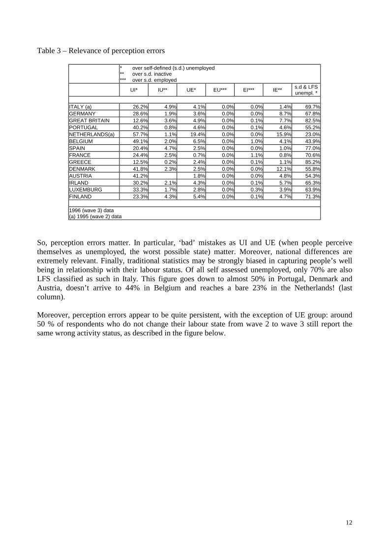
In some sense, the UI groups are the most problematic, since someone who perceives himself as unemployed but does not struggle to find a job is likely to share the same unhappiness and frustration of a ‘real’ unemployed, but with a smaller probability to get out of this state. It is clear that the first perception error (no search at all) is much worse than the second (passive search). People in the IU group can be labelled as ‘unaware’: we expect them to be included in a social safety net that lessens the harsh of unemployment. Being in this group is a priori no good or bad, but a sign of (relative) ‘good luck’, with possibly a positive impact on the overall well being of the individual. Finally, as described above, being in the UE or IE group can signal a particular active attitude with respect to unemployment or exclusion from the labour force, but also a lack of interest in the part-time job, if our first hypothesis turns out to be correct. The first attitude is clearly ‘positive’ from a social perspective. On the other hand, in the “lack of centrality” hypothesis it is the situation of the non misperceptors – those that show a strong interest in their part-time job – that can be problematic, since some of them could be forced to make their living out of a part-time work, while still preferring a full time occupation7. 3. The relevance of misperception But how relevant are these perception errors? The table below shows that 26.2% of all people who perceive themselves as unemployed are recorded as inactive by the official statistics provided by the national statistical office (“Indagine trimestrale sulla forza lavoro”) in Italy, thus committing a UI type perception error. The frequency of this misperception goes as high as 57.7% in the Netherlands, 49.1% in Belgium and just above 40% in Denmark, Austria and Portugal, while it goes down to 12.6% in Great Britain and 12.5% in Greece. Conversely, 4.9% of all people declaring to be inactive are (‘officially’) unemployed in Italy. This figure remains high for Spain (4.7%) and Finland (4.3%), reaching a low of 0.8% in Portugal and 0.2% in Greece. Moreover, in Italy 4.1% of self assessed unemployed are ‘officially’ working, a perception error committed by 19.4% of self assessed unemployed in the Netherlands, and by just 0.7% in France. Finally, only 1.4% of self assessed inactive are ‘officially’ working in Italy, while in the Netherlands this figure is as high as 15.9%, in Denmark reaches 12.9%, and it goes down to around 1% in Spain and Greece, and to 0.8% in France.

7 many people choose to work part-time as the optimal choice given their other activities (like bearing children, or simply enjoying rents), but we suppose that most people declaring to be part-time workers are forced to make this choice, and would opt for a full-time, if they could.

12

Table 3 – Relevance of perception errors

* over self-defined (s.d.) unemployed ** over s.d. inactive *** over s.d. employed

UI* IU** UE* EU*** EI*** IE** s.d & LFS unempl. *

ITALY (a) 26.2% 4.9% 4.1% 0.0% 0.0% 1.4% 69.7% GERMANY 28.6% 1.9% 3.6% 0.0% 0.0% 8.7% 67.8% GREAT BRITAIN 12.6% 3.6% 4.9% 0.0% 0.1% 7.7% 82.5% PORTUGAL 40.2% 0.8% 4.6% 0.0% 0.1% 4.6% 55.2% NETHERLANDS(a) 57.7% 1.1% 19.4% 0.0% 0.0% 15.9% 23.0% BELGIUM 49.1% 2.0% 6.5% 0.0% 1.0% 4.1% 43.9% SPAIN 20.4% 4.7% 2.5% 0.0% 0.0% 1.0% 77.0% FRANCE 24.4% 2.5% 0.7% 0.0% 1.1% 0.8% 70.6% GREECE 12.5% 0.2% 2.4% 0.0% 0.1% 1.1% 85.2% DENMARK 41.8% 2.3% 2.5% 0.0% 0.0% 12.1% 55.8% AUSTRIA 41.2% 1.8% 0.0% 0.0% 4.8% 54.3% IRLAND 30.2% 2.1% 4.3% 0.0% 0.1% 5.7% 65.3% LUXEMBURG 33.3% 1.7% 2.8% 0.0% 0.3% 3.9% 63.9% FINLAND 23.3% 4.3% 5.4% 0.0% 0.1% 4.7% 71.3%

1996 (wave 3) data (a) 1995 (wave 2) data

So, perception errors matter. In particular, ‘bad’ mistakes as UI and UE (when people perceive themselves as unemployed, the worst possible state) matter. Moreover, national differences are extremely relevant. Finally, traditional statistics may be strongly biased in capturing people’s well being in relationship with their labour status. Of all self assessed unemployed, only 70% are also LFS classified as such in Italy. This figure goes down to almost 50% in Portugal, Denmark and Austria, doesn’t arrive to 44% in Belgium and reaches a bare 23% in the Netherlands! (last column). Moreover, perception errors appear to be quite persistent, with the exception of UE group: around 50 % of respondents who do not change their labour state from wave 2 to wave 3 still report the same wrong activity status, as described in the figure below.

13

Table 4 – Persistence of perception errors: erception flows of people who do not change their ILO labour state from wave 2 to wave 3

The fact that what counts, in terms of personal well being, is the perceived labour status, rather than the true labour status (as classified by LFS standards) is confirmed when looking at the correlation of perception errors and satisfaction level8. Perceiving to be unemployed is worse than perceiving to be inactive, given (LFS) inactivity; conversely, perceiving to be inactive is better than perceiving to be unemployed, given (LFS) unemployment. Moreover, perceiving to be unemployed is worse – and perceiving to be inactive better – than perceiving to be a part-time worker, given the individual is an (LFS) part-time worker.

8 the questionnaire asks about the satisfaction with work or main activity, ranging from 1 – not satisfied – to 6 – fully satisfied.

14

Figure 1 – Diffusion of perception errors and satisfaction levels

UI are in % of all inactive, IU are in % of all unemployedUE are in % of all non-IE part-time workers, IE are in % of all non-UE part-time workers

Misperception & Satisfaction

0

5

10

15

20

25

30

35

1 2 3 4 5 6Satisfaction level

Mis

perc

eptio

n (%

)

UI IU

Misperception & Satisfaction

0102030405060708090

100

1 2 3 4 5 6

Satisfaction level

Mis

perc

eptio

n (%

)

UE IE

A first look at the numbers above could suggest a stereotypical interpretation, going down more or less like this: “Family links in Italy and Spain are stronger, and thus unemployed persons are more likely not to perceive the harshness of their status (high frequency of IU misperception); individualism in Great Britain is strong, and thus people tend not to blame others for their personal situation, while in Greece this may be due to a weaker state (low frequency of UI misperception); labour legislation favouring part-time in the Netherlands explain the sky-high frequency of UE and IE misperception in this country”. The remaining of the paper is devoted to better qualify this. 4. Misperception and labour force statistics At this point, it could be asked how it is possible to rely on traditional statistics as the unemployment rate, when overall only around 3 in 4 people who feel unemployed are counted in. The fact is: ‘official statistics’ do not necessarily reflect what people feel, they are measuring something else. Moreover, some perception errors offset each other. Self-definition and LFS classification are linked by the following identities:

[4] s.d. unemployed = LFS unemployed – IU – EU + UI + UE [5] s.d. employed = LFS employed – IE – UE + EI + EU [6] s.d. inactive = LFS inactive – UI – EI + IU + IE

Let’s confine our attention to the first one. Since EU = 0, it reduces to

[4’] s.d. unemployed = LFS unemployed – IU + UI + UE The intersection set – i.e. the set of people who are at the same time both self assessed and LFS unemployed – is small compared to the self assessed set when UI and UE misperception are large, and is small compared to the LFS set when IU is large.

15

Figure 2 – LFS and self assessed unemployment However, even if IU, UI and UE may partially offset each other, when statistics based on LFS classification are to be used as an estimate for self-perceived unemployment, the risk of big mistakes remains high: Table 5 – Difference between self assessed unemployment and LFS unemployment

Difference * ITALY (a) 2.2% GERMANY 15.1% GREAT BRITAIN -24.8% PORTUGAL 36.9% NETHERLANDS(a) 72.6% BELGIUM 43.9% SPAIN 0.7% FRANCE 12.9% GREECE 13.5% DENMARK 30.9% AUSTRIA 20.4% IRLAND 19.7% LUXEMBURG -5.6% FINLAND 13.1%

* (s.d unemployment – LFS unemployment) over LFS unemployment

5. The regional dimension We have seen that perception errors differ greatly across countries. They also differ within countries, across regions. We want to investigate how and why this happens. However, the number of observations is too small to allow a ‘true’ regional analysis (due to the relative small incidence of each type of perception error). We need then a territorial criterion to aggregate regions. We used the EU structural funds objective 1, 2 and 5b eligibility status of each region. These objectives are the only geographical objectives of the 1996-2001 structural funds, since obj. 3, 5a and 6 refer to any EU region, regardless of its characteristics. Objective 1 was aimed to promoting the development and structural adjustment of the EU regions most lagging behind in development, while Objective 2

IU UI +

UE

self assessed unemployed LFS unemployed

16

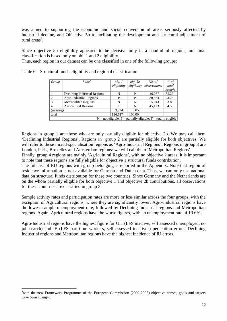
was aimed to supporting the economic and social conversion of areas seriously affected by industrial decline, and Objective 5b to facilitating the development and structural adjustment of rural areas9. Since objective 5b eligibility appeared to be decisive only in a handful of regions, our final classification is based only on obj. 1 and 2 eligibility. Thus, each region in our dataset can be one classified in one of the following groups: Table 6 – Structural funds eligibility and regional classification

Group Label obj. 1 eligibility

obj. 2b eligibility

No. of observations

% of total

sample 1 Declining Industrial Regions N P 46,087 35.29 2 Agro-Industrial Regions P P 30,364 23.25 3 Metropolitan Regions N N 5,043 3.86 4 Agricultural Regions T N 45,123 34.55 (missing) 3,994 3.05 total 126,617 100.00

N = not eligible; P = partially eligible; T = totally eligible

Regions in group 1 are those who are only partially eligible for objective 2b. We may call them ‘Declining Industrial Regions’. Regions in group 2 are partially eligible for both objectives. We will refer to these mixed-specialisation regions as ‘Agro-Industrial Regions’. Regions in group 3 are London, Paris, Bruxelles and Amsterdam regions: we will call them ‘Metropolitan Regions’. Finally, group 4 regions are mainly ‘Agricultural Regions’, with no objective 2 areas. It is important to note that these regions are fully eligible for objective 1 structural funds contribution. The full list of EU regions with group belonging is reported in the Appendix. Note that region of residence information is not available for German and Dutch data. Thus, we can only use national data on structural funds distribution for these two countries. Since Germany and the Netherlands are on the whole partially eligible for both objective 1 and objective 2b contributions, all observations for these countries are classified in group 2. Sample activity rates and participation rates are more or less similar across the four groups, with the exception of Agricultural regions, where they are significantly lower. Agro-Industrial regions have the lowest sample unemployment rate, followed by Declining Industrial regions and Metropolitan regions. Again, Agricultural regions have the worse figures, with an unemployment rate of 13.6%. Agro-Industrial regions have the highest figure for UI1 (LFS inactive, self assessed unemployed, no job search) and IE (LFS part-time workers, self assessed inactive ) perception errors. Declining Industrial regions and Metropolitan regions have the highest incidence of IU errors.

9with the new Framework Programme of the European Commission (2002-2006) objective names, goals and targets have been changed

17

Table 7 – Misperception and regional classification

Macro-regions Misperception Declining Industrial Agro-Industrial Metropolitan Agricultural

UI1 * 355 1.9% 672 5.5% 54 2.6% 477 2.2% UI2 * 332 1.8% 203 1.7% 35 1.7% 389 1.8% IU ** 574 24.7% 248 19.1% 65 24.0% 558 17.4% UE *** 105 0.4% 207 1.2% 7 0.3% 121 0.6% IE *** 820 3.2% 1008 6.0% 36 1.3% 561 2.7% participation rate 60.2% 59.5% 58.7% 52.4% unemployment rate 8.4% 7.2% 9.2% 13.6% activity rate 55.1% 55.2% 53.3% 45.3% * over inactive ** over unemployed *** over employed

6. The determinants of misperception We do not provide a formal theory of misperception. We simply divide the determinants of misperception in three categories:

• institutional determinants • economic determinants, and • social determinants

Institutional factors refer to those situations when there is a social recognition of a particular labour status (as in the case of unemployment benefits, or pensions). It can happen that LFS classification does not correspond to this ‘social visa’. For instance, one person can receive a scholarship, but still work a few hours a week in order to increase his/her income. In such cases, we expect the existence of these allowances to increase the probability of a misperception. Economic and social factors affect misperception in many ways. To start with, they normally affect the institutional factors10. In the case of the UI group, they are directly linked with the ‘victimisation hypothesis’, according to which beyond a certain threshold of (perceived) economic and social distress individuals tend to blame the society for their personal situation, and thus switch the responsibility for an improvement from themselves to the state. In the case of IU group, they are connected with the safety net effect described above. In order to investigate the determinants of the four categories of misperception described above, we run separate logit regressions, comparing each misperception group with the corresponding correct perception group. Thus, our logit regression for the UI compares being an UI with being a II, i.e. declaring to be unemployed versus declaring to be inactive, given that the individual is classified as an LFS inactive. The logit regression for the IU compares declaring to be inactive versus declaring to be unemployed, given that the individual is classified as an LFS unemployed, and so forth. Note that UE and IE are both regressed against EE: thus, IE observations are excluded from UE regression, and vice versa.

10 but since this causal relationship differ from country to country due to different legislation on social protection – and we put observations from different countries together – it is still convenient to include the institutional factors among the regressors.

18

Regressors include personal information – sex, age, citizenship, legal status (whether one is married), instruction – household information – dimension of household, existence of children to be cared of, location in an area with crime or vandalism problems – and income information. Now, it is important to note that misperception may reveal something about work determination, and thus about unobservable ability. In the case of the UI group for example, it is intuitive to link misperception to the individual being a ‘low type’ worker. Including income information among the regressors could thus lead to an endogeneity problem, since income may in turn depend on such determination, or unobserved ability (and thus on the perception error). Fortunately, this is not the case in the UI and IU regressions, since we are confident to assume that being an UI rather than an II – or a IU rather than a UU – does not affect income. The main reason is that there is no work income here. Non-work private income (capital income, private transfers) can be thought to be independent of whether one admits or not to be inactive, or unemployed11. Unemployment benefits and other social receipts are not generally granted after a simple declaration to be unemployed. Conversely, IE and UE regressions are affected by this endogeneity problem, which introduces a correlation between work income and the errors. We tackle this problem by instrumenting income in the IE and UE regressions. Although the questionnaire asks important questions about health status and satisfaction level, we do not include any of these variables among the regressors, since the number of missing data becomes significant, and selection biases could be introduced. Country dummies are included. The full list of variables used in the regressions is reported in the table below: Table 8 – Explanatory variables Code Description dummy UI IU UE IE IV income PE003 LFS MAIN ACTIVITY DURING CURRENT YEAR pe003_4 * discouraged * x o PE005 TOTAL HOURS WORKING / WEEK o o o pe005sq squared o o o HD004 EQUIVALISED SIZE, OECD SCALE o o o HI100ecu TOTAL NET HOUSEHOLD INCOME o o o o hi100esq squared o o o o PI110ECU TOTAL NET INCOME FROM WORK o o pi110esq squared o o PI131ecu UNEMPLOYMENT RELATED BENEFITS o o o PI131esq squared o o o PI132ecu OLD-AGE / SURVIVORS' BENEFITS o o o PI132esq squared o o o PI133ECU FAMILY-RELATED ALLOWANCES o o o PI133esq squared o o o PI134ECU SICKNESS/INVALIDITY BENEFITS o o o PI134esq squared o o o PI135ECU EDUCATION-RELATED ALLOWANCES o o o PI135esq squared o o o HF002 IS THE HOUSEHOLD ABLE TO MAKE ENDS MEET hf002_no * with some difficulty - with great difficulty * o o

HF013 MONEY LEFT FOR THE HOUSEHOLD TO SAVE (CONSIDERING HOUSEHOLD'S INCOME AND EXPENSES)

hf013_2 * no or very little * x o o o o HA022 IS THERE CRIME OR VANDALISM IN THE AREA

11 non-work income could depend on whether one is unemployed rather that inactive. For instance, inactive people could have decided to drop out of the labour force exactly because of sufficient capital income. Elderly people could receive private transfers from their relatives. But the distinction here is whether one declares to be unemployed, rather than inactive.

19

ha022_1 * yes * x o o o o o HL002 CHILDREN LOOKED AFTER ON A REGULAR BASIS hl002_1 * yes * x o o o o PD003 AGE OF THE INDIVIDUAL o o o o o pd003sq squared o o o o o PD004 SEX OF THE INDIVIDUAL pd004_2 * female * x o o o o o PD005 MARITAL STATUS OF THE PERSON pd005_1 * married * x o o o o PT001 HAS THE PERSON BEEN IN EDUCATION OR TRAINING RECENTLY pt001_1 * yes * x o o o

PT022 HIGHEST LEVEL OF GENERAL OR HIGHER EDUCATION COMPLETED

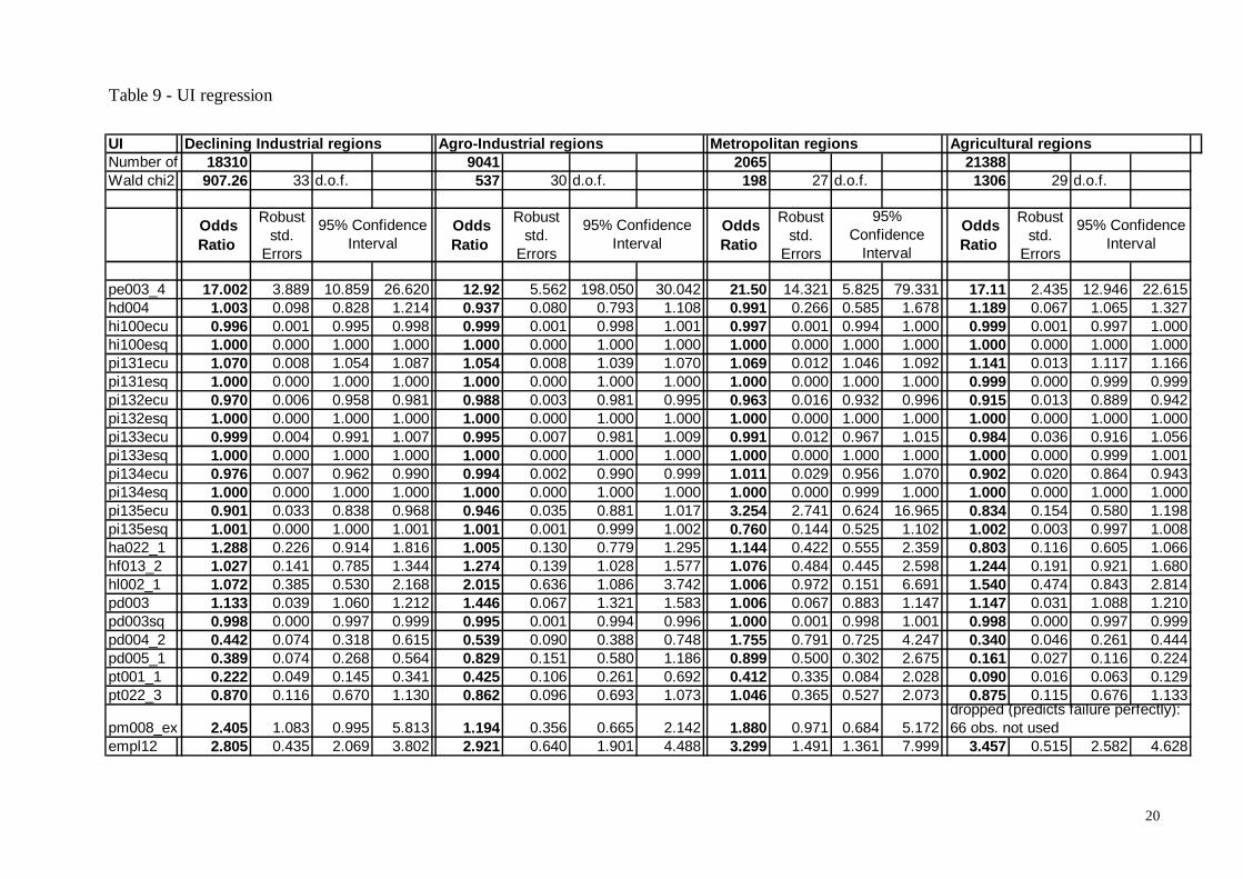
pt022_3 * Less than second stage of secondary education * x o o o o PH001 HEALTH OF THE PERSON IN GENERAL o PM008 CITIZENSHIP pm008_ex * Other citizenship (Extra-EU) or Not national, but citizenship unkown * x o o o o o EMPL12 S.D. EMPLOYED IN THE LAST 12 MONTHS x o o PE017 USE OF A FOREIGN LANGUAGE IN CURRENT JOB pe017_1 * yes * o The UI group A fundamental variable we introduce in the regression of the likelihood of declaring to be unemployed, when inactive, is whether the individual does not search for a job because he/she is discouraged. We expect being discouraged to affect positively this likelihood. As it turns out, this is the single most important factor in explaining this type of misperception. Among the income variables, we include data on total net household income and on personal social allowances. Household income could affect UI misperception in two ways: living in a poor household could increase awareness and personal responsibility, and thus lower the likelihood of a misperception, or it could increase the attribution of the ultimate responsibility of such an uncomfortable situation to the state, and thus increase the likelihood of a misperception. Hence, a positive coefficient would support the ‘victimisation hypothesis’. The same applies to other indicators of social distress, such as localisation in a low-security area and a dummy variable signalling whether the household does not manage to save money. Social receipts are introduced as control variables. Unfortunately, since German data on these income variables are missing, we have to drop all German observations from our sample. We run a separate regression for this country12, and investigate whether the other effects differ significantly from other Agro-Industrial regions (recall all German observations belong to the same group, since region of living information is also missing). We obviously expect unemployment benefits to increase the likelihood of a misperception, and other social allowances related to inactivity status to decrease it. However, the size of these effects and their variability across regions could shed light on the importance of what we called the ‘institutional effect’.

12 data are available on request

20

UINumber of 18310 9041 2065 21388Wald chi2 907.26 33 d.o.f. 537 30 d.o.f. 198 27 d.o.f. 1306 29 d.o.f.

Odds Ratio

Robust std.

Errors

Odds Ratio

Robust std.

Errors

Odds Ratio

Robust std.

Errors

Odds Ratio

Robust std.

Errors

pe003_4 17.002 3.889 10.859 26.620 12.92 5.562 198.050 30.042 21.50 14.321 5.825 79.331 17.11 2.435 12.946 22.615hd004 1.003 0.098 0.828 1.214 0.937 0.080 0.793 1.108 0.991 0.266 0.585 1.678 1.189 0.067 1.065 1.327hi100ecu 0.996 0.001 0.995 0.998 0.999 0.001 0.998 1.001 0.997 0.001 0.994 1.000 0.999 0.001 0.997 1.000hi100esq 1.000 0.000 1.000 1.000 1.000 0.000 1.000 1.000 1.000 0.000 1.000 1.000 1.000 0.000 1.000 1.000pi131ecu 1.070 0.008 1.054 1.087 1.054 0.008 1.039 1.070 1.069 0.012 1.046 1.092 1.141 0.013 1.117 1.166pi131esq 1.000 0.000 1.000 1.000 1.000 0.000 1.000 1.000 1.000 0.000 1.000 1.000 0.999 0.000 0.999 0.999pi132ecu 0.970 0.006 0.958 0.981 0.988 0.003 0.981 0.995 0.963 0.016 0.932 0.996 0.915 0.013 0.889 0.942pi132esq 1.000 0.000 1.000 1.000 1.000 0.000 1.000 1.000 1.000 0.000 1.000 1.000 1.000 0.000 1.000 1.000pi133ecu 0.999 0.004 0.991 1.007 0.995 0.007 0.981 1.009 0.991 0.012 0.967 1.015 0.984 0.036 0.916 1.056pi133esq 1.000 0.000 1.000 1.000 1.000 0.000 1.000 1.000 1.000 0.000 1.000 1.000 1.000 0.000 0.999 1.001pi134ecu 0.976 0.007 0.962 0.990 0.994 0.002 0.990 0.999 1.011 0.029 0.956 1.070 0.902 0.020 0.864 0.943pi134esq 1.000 0.000 1.000 1.000 1.000 0.000 1.000 1.000 1.000 0.000 0.999 1.000 1.000 0.000 1.000 1.000pi135ecu 0.901 0.033 0.838 0.968 0.946 0.035 0.881 1.017 3.254 2.741 0.624 16.965 0.834 0.154 0.580 1.198pi135esq 1.001 0.000 1.000 1.001 1.001 0.001 0.999 1.002 0.760 0.144 0.525 1.102 1.002 0.003 0.997 1.008ha022_1 1.288 0.226 0.914 1.816 1.005 0.130 0.779 1.295 1.144 0.422 0.555 2.359 0.803 0.116 0.605 1.066hf013_2 1.027 0.141 0.785 1.344 1.274 0.139 1.028 1.577 1.076 0.484 0.445 2.598 1.244 0.191 0.921 1.680hl002_1 1.072 0.385 0.530 2.168 2.015 0.636 1.086 3.742 1.006 0.972 0.151 6.691 1.540 0.474 0.843 2.814pd003 1.133 0.039 1.060 1.212 1.446 0.067 1.321 1.583 1.006 0.067 0.883 1.147 1.147 0.031 1.088 1.210pd003sq 0.998 0.000 0.997 0.999 0.995 0.001 0.994 0.996 1.000 0.001 0.998 1.001 0.998 0.000 0.997 0.999pd004_2 0.442 0.074 0.318 0.615 0.539 0.090 0.388 0.748 1.755 0.791 0.725 4.247 0.340 0.046 0.261 0.444pd005_1 0.389 0.074 0.268 0.564 0.829 0.151 0.580 1.186 0.899 0.500 0.302 2.675 0.161 0.027 0.116 0.224pt001_1 0.222 0.049 0.145 0.341 0.425 0.106 0.261 0.692 0.412 0.335 0.084 2.028 0.090 0.016 0.063 0.129pt022_3 0.870 0.116 0.670 1.130 0.862 0.096 0.693 1.073 1.046 0.365 0.527 2.073 0.875 0.115 0.676 1.133

pm008_ex 2.405 1.083 0.995 5.813 1.194 0.356 0.665 2.142 1.880 0.971 0.684 5.172empl12 2.805 0.435 2.069 3.802 2.921 0.640 1.901 4.488 3.299 1.491 1.361 7.999 3.457 0.515 2.582 4.628

Table 9 - UI regression

dropped (predicts failure perfectly): 66 obs. not used

Declining Industrial regions Agro-Industrial regions Metropolitan regions Agricultural regions

95% Confidence Interval

95% Confidence Interval

95% Confidence

Interval

95% Confidence Interval

21

The discouragement effect and the victimisation hypothesis As we anticipated, discouragement is the single most important factor in explaining this type of misperception. Being discouraged increases the odds ratio of an order of magnitude. The effect is stronger in Metropolitan regions, which is what it would be expected. Discouraged people don’t consider themselves completely out of the labour force: they simply assume a more passive attitude. If we think of human action as the ability of using tools in order to reach goals (either consciously or unconsciously) we could say that the process of dropping out of the labour force involves two stages. People first loose the tool, then the goal itself. This is confirmed by the fact that almost 63% of all discouraged people in our sample declare to be unemployed. Age is also very important, with a 13% increase in the odds ratio in Declining Industrial regions for each additional year, and almost 50% increase in Agro-Industrial regions. This can be interpreted following the discouragement hypothesis. As times goes by, search efforts are reduced. Moreover, if actions are decided rationally, they should be positively linked to their expected benefits. Since search is costly (and it becomes even more so with age), the likelihood of getting a job decreases with age, and expected benefits from a job also decrease (at least because expected remaining lifetime decreases) the intensity of the job search should diminish. When it falls below a threshold, the individual is not classified anymore as unemployed by LFS rules, while continuing to be interested in getting a job. The other side of this psychological interpretation is that a recent period of work should increase the feeling of being unemployed, even if no search is conducted. In some sense, we could say that long-term unemployed share with recently unemployed people the same tendency to ‘passive’ behaviour. Individuals keep a ‘memory’ of what they recently did, and this affects the perception of their present situation. Thus, if they were unemployed, it is likely that they hold the impression they should still be considered so, even if they are not performing an active search anymore. On the other hand, if they were employed, it is possible that they hold the impression they should be given another job, no matter what they do in order to get it. The result is the same: an inclination towards UI type misperception. This is confirmed by the positive coefficient of the variable ‘empl12’ (a dummy signalling whether the individual declared at least once to be employed in the 12 months preceding the interview), with a three times increase in the odds ratio. Having reached the goal (of a job) once can induce people to think they gained a permanent right to it. This is clearly linked with the ‘victimisation hypothesis’ we already introduced. When people stop searching for a job, while still thinking they are entitled to one, they are assuming the society should take care for themselves. There are other pieces of evidence supporting this interpretation. First of all, total household income affects misperception in a negative (and almost linear over the range considered) way. Poor people are thus more likely to be affected by a UI perception error. Immigrants are slightly less likely to commit this error13, coherently with the intuition they have probably less claims towards a society that is already hosting them. Since the victimisation hypothesis is strongly linked to the concept of responsibility, we should expect UI misperception to be less common in more liberal countries, where the stress on individualism is stronger. We believe this phenomenon is partly due to cultural reasons and education, and partly to the fact that discouragement becomes more costly when the social safety net is weaker. Thus, discouragement should be less common in more liberal countries14. This trend is found in the data: being in Great Britain for instance reduces the odds ratio by a half in Declining 13 in Germany very are more likely to commit it, with an odds ratio 3 times higher. 14 on the other side, deep discouragement could well be more widespread

22

Industrial regions and Agricultural regions, and by almost a factor of ten in Agro-Industrial regions15. On the opposite, living in more socialist countries like Belgium, the Netherlands, Denmark or Finland increases the odds ratio by two to three times. Women are much less likely to commit a UI error (odds ratio are reduced by roughly a half16). Only in Metropolitan regions this effect is not relevant, as gender becomes less important in determining attitude towards life in general. Also, being married reduces the likelihood of an error. The effect is stronger in Agricultural regions, where marriage is a stronger social convention, and is not relevant in Metropolitan regions, where it is weaker. Moreover, the discouragement effect is much stronger for males than for females. Its multiplicative effect on the odds ratio is 2 to 5 times stronger for males than for females. Age also has a stronger effect for males. Also, the discouragement effect is very strong in Germany, with more of 60 times increase in the odds ratio. Institutional factors While having a low educational level does not alter significantly the likelihood of making a UI type misperception, having been in education or training in the months before the interview reduces it dramatically17. In Agricultural regions this effect amounts to a tenfold reduction, in Declining Industrial regions it amounts to a four times reduction, while in the other regions it halves the likelihood of an error. Institutional factors affect the odds ratio in the way we presumed. Each one hundred ecus increase in unemployment benefits increases it by 5 to 7 percent (14% in Agricultural regions). The effect is almost linear. On the other hand, each one hundred ecus increase in old age and survivor’s benefits decreases the odds ratio by 2 to 4 percent (almost 10% in Agricultural regions). Sickness and invalidity benefits have an effect similar to that of pensions, with a decrease of the odds ratio of 1 to 2 percent (almost 10% in Agricultural regions) every 100 ecus increase in the benefits. Education related allowances do not appear to be significant in most regions. When they are, they decrease the odds ratio, as expected. The interesting thing here is that socio-institutional factors (education and social benefits) have a much stronger effect in Agricultural regions. These are more traditional societies, where the distinction of different roles is probably more relevant. No search and bad search When running separate regressions for UI1 (no search) and UI2 (no active search) groups, the main thing to be noted is that the discouragement effect appears not to be significant for the first group, while very strong for the latter. This is highly reasonable, and confirms our interpretation that UI2 group is partly made of ‘latent unemployed’. Bring just a little degree of confidence to the 42% of UI2 guys who declare to be discouraged, and they will be classified as unemployed. Overall, unemployment figure in the EU could go up as high as 0.6% because of this effect.

15 due to collinearity, some country dummies are dropped in each regressions. 16 data on gender regressions are available on request 17 we include this variable among the institutional factors since it involves a ‘formal’ recognition of an inactivity status. This is clearly very different from the overall level of education.

23

Table 10 – Discouragement and search

UI1 UI2 discouraged 10.0 % 42.1 % other inactive 90.0 % 57.9 % total 100.0 % 100.0 %

Table 11 – UI1 and UI2 misperception logit regressions: Selected coefficients

O.R. std. Errors O.R. std.

Errors O.R. std. Errors O.R. std.

Errors

pe003_4 1.42 0.70 0.54 3.73 25.49 5.78 16.34 39.76 0.38 0.21 0.13 1.12 28.22 10.85 13.29 59.95hi100ecu 1.00 0.00 0.99 1.00 1.00 0.00 0.99 1.00 1.00 0.00 1.00 1.00 1.00 0.00 1.00 1.01pd003 1.12 0.04 1.04 1.21 1.19 0.06 1.07 1.32 1.34 0.06 1.23 1.46 1.70 0.14 1.44 1.99pd004_2 0.45 0.10 0.29 0.69 0.51 0.11 0.33 0.78 0.62 0.10 0.45 0.86 0.51 0.16 0.28 0.94pd005_1 0.44 0.10 0.28 0.68 0.45 0.12 0.27 0.75 0.79 0.14 0.56 1.12 1.02 0.38 0.49 2.11pt001_1 0.17 0.05 0.09 0.29 0.43 0.11 0.26 0.71 0.32 0.09 0.18 0.55 1.07 0.42 0.50 2.30empl12 2.40 0.51 1.58 3.64 2.51 0.52 1.67 3.76 2.71 0.66 1.69 4.35 2.16 0.75 1.09 4.29

O.R. std. Errors O.R. std.

Errors O.R. std. Errors O.R. std.

Errors

pe003_4 0.43 0.41 0.08 3.22 49.61 33.28 13.32 184.74 1.65 0.34 1.10 2.46 20.28 3.34 14.69 28.00hi100ecu 1.00 0.00 1.00 1.01 1.00 0.00 0.99 1.00 1.00 0.00 1.00 1.00 1.00 0.00 1.00 1.00pd003 0.97 0.09 0.81 1.17 1.16 0.14 0.92 1.46 1.16 0.04 1.09 1.23 1.11 0.04 1.02 1.20pd004_2 1.07 0.57 0.38 3.04 2.89 1.81 0.85 9.88 0.37 0.06 0.27 0.51 0.49 0.09 0.34 0.71pd005_1 2.03 1.41 0.52 7.88 0.53 0.38 0.13 2.18 0.20 0.04 0.13 0.30 0.28 0.06 0.19 0.43pt001_1 0.46 0.36 0.10 2.11 0.55 0.61 0.06 4.80 0.16 0.04 0.10 0.26 0.10 0.03 0.06 0.17empl12 1.48 0.91 0.45 4.92 5.40 3.86 1.33 21.92 2.85 0.47 2.06 3.93 0.83 0.15 0.58 1.18

Declining Industrial regions Agro-Industrial regionsUI1 UI2 UI1 UI2

95% Confidence

Interval

95% Confidence

Interval

18335 18335 9049 9049

Agricultural regionsUI1 UI2 UI1 UI2

95% Confidence

Interval

95% Confidence

Interval

1951 2065 21291 21421

Number of obs.

Number of obs.

95% Confidence

Interval

95% Confidence

Interval

Metropolitan regions

95% Confidence

Interval

95% Confidence

Interval

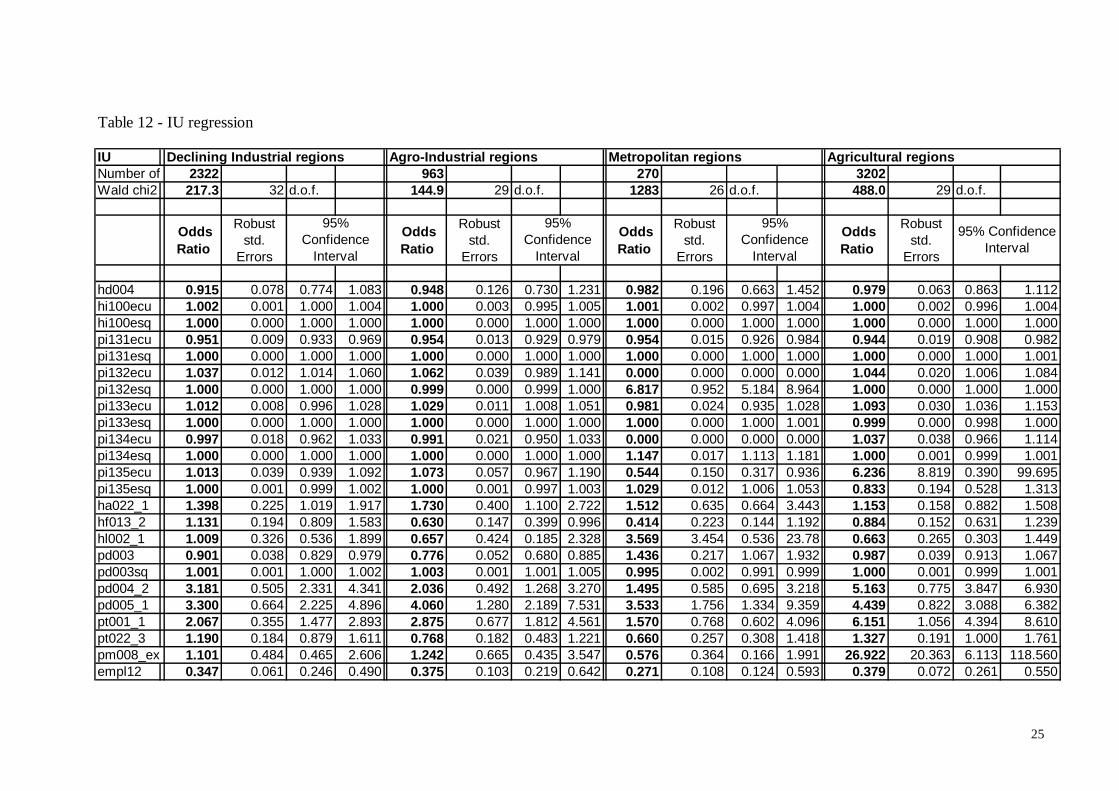
The IU group When regressing for the IU misperception group (those who declare to be inactive, but are classified as LFS unemployed, since they perform a correct job search), we have to drop the discouragement variable (LFS inactive because discouraged), since it is clearly correlated with the dependent variable (1 if LFS inactive, 0 otherwise). All other variables are the same we used for the UI regressions. In some sense this perception error is the opposite of the UI one. Here, people are underemphasizing their efforts, rather than overemphasizing them: we thus expect most variables to affect the odds ratio in the opposite direction. However, evidence on the discouragement effect is mixed. On one hand, total household income, as well as the savings dummy, are not significant. On the other hand, the age effect and the previous-employment effect confirm our hypothesis. In analysing the UI group, we found out that older people tend to overemphasise, and we related this to the discouragement effect. Here, data show that older people are less likely to underemphasise (commit a IU error): the effect is quite

24

important, with a decrease in the odds ratio that can reach –20% in Agro-Industrial regions. Moreover, it is much more significant for men then for women. Having experienced a period of employment in the 12 months before the interview slashes the odds ratio to roughly a third. The other effects also work in the way we supposed, i.e. in the opposite direction relative to the UI group. Each 100 ecus increase in unemployment benefits reduces the likelihood of a IU perception error of around 5%, while each 100 ecus increase in pensions increases it of 2-4%, thus confirming the existence of an important institutional effect. Family related allowances are important only in Agricultural regions, where they increase the odds ratio of almost 10%. Everywhere, being a woman increases the likelihood of a IU misperception (from 2 to as high as 5 times) 18. Also, being married leads to a 3 to 4 times increase, and this is particular true for women. This could be due, as for the UI misperception, to a smaller need for employment due to a social and family structure that, to a certain extent, takes care of women, and to cultural traditions suggesting a woman to declare to be inactive (student, involved with housework…), rather than unemployed, even if she is looking for a job. The separate regression for German observations (see above) is of no special interest.19

18 data on gender regressions are available on request 19 data are available on request. The only striking feature is the effect of the dummy indicating possession of a home computer, which is significant and positive (odds ratio increased by a factor of 7!).

25

Table 12 - IU regression

IUNumber of 2322 963 270 3202Wald chi2 217.3 32 d.o.f. 144.9 29 d.o.f. 1283 26 d.o.f. 488.0 29 d.o.f.

Odds Ratio

Robust std.

Errors

Odds Ratio

Robust std.

Errors

Odds Ratio

Robust std.

Errors

Odds Ratio

Robust std.

Errors

hd004 0.915 0.078 0.774 1.083 0.948 0.126 0.730 1.231 0.982 0.196 0.663 1.452 0.979 0.063 0.863 1.112hi100ecu 1.002 0.001 1.000 1.004 1.000 0.003 0.995 1.005 1.001 0.002 0.997 1.004 1.000 0.002 0.996 1.004hi100esq 1.000 0.000 1.000 1.000 1.000 0.000 1.000 1.000 1.000 0.000 1.000 1.000 1.000 0.000 1.000 1.000pi131ecu 0.951 0.009 0.933 0.969 0.954 0.013 0.929 0.979 0.954 0.015 0.926 0.984 0.944 0.019 0.908 0.982pi131esq 1.000 0.000 1.000 1.000 1.000 0.000 1.000 1.000 1.000 0.000 1.000 1.000 1.000 0.000 1.000 1.001pi132ecu 1.037 0.012 1.014 1.060 1.062 0.039 0.989 1.141 0.000 0.000 0.000 0.000 1.044 0.020 1.006 1.084pi132esq 1.000 0.000 1.000 1.000 0.999 0.000 0.999 1.000 6.817 0.952 5.184 8.964 1.000 0.000 1.000 1.000pi133ecu 1.012 0.008 0.996 1.028 1.029 0.011 1.008 1.051 0.981 0.024 0.935 1.028 1.093 0.030 1.036 1.153pi133esq 1.000 0.000 1.000 1.000 1.000 0.000 1.000 1.000 1.000 0.000 1.000 1.001 0.999 0.000 0.998 1.000pi134ecu 0.997 0.018 0.962 1.033 0.991 0.021 0.950 1.033 0.000 0.000 0.000 0.000 1.037 0.038 0.966 1.114pi134esq 1.000 0.000 1.000 1.000 1.000 0.000 1.000 1.000 1.147 0.017 1.113 1.181 1.000 0.001 0.999 1.001pi135ecu 1.013 0.039 0.939 1.092 1.073 0.057 0.967 1.190 0.544 0.150 0.317 0.936 6.236 8.819 0.390 99.695pi135esq 1.000 0.001 0.999 1.002 1.000 0.001 0.997 1.003 1.029 0.012 1.006 1.053 0.833 0.194 0.528 1.313ha022_1 1.398 0.225 1.019 1.917 1.730 0.400 1.100 2.722 1.512 0.635 0.664 3.443 1.153 0.158 0.882 1.508hf013_2 1.131 0.194 0.809 1.583 0.630 0.147 0.399 0.996 0.414 0.223 0.144 1.192 0.884 0.152 0.631 1.239hl002_1 1.009 0.326 0.536 1.899 0.657 0.424 0.185 2.328 3.569 3.454 0.536 23.78 0.663 0.265 0.303 1.449pd003 0.901 0.038 0.829 0.979 0.776 0.052 0.680 0.885 1.436 0.217 1.067 1.932 0.987 0.039 0.913 1.067pd003sq 1.001 0.001 1.000 1.002 1.003 0.001 1.001 1.005 0.995 0.002 0.991 0.999 1.000 0.001 0.999 1.001pd004_2 3.181 0.505 2.331 4.341 2.036 0.492 1.268 3.270 1.495 0.585 0.695 3.218 5.163 0.775 3.847 6.930pd005_1 3.300 0.664 2.225 4.896 4.060 1.280 2.189 7.531 3.533 1.756 1.334 9.359 4.439 0.822 3.088 6.382pt001_1 2.067 0.355 1.477 2.893 2.875 0.677 1.812 4.561 1.570 0.768 0.602 4.096 6.151 1.056 4.394 8.610pt022_3 1.190 0.184 0.879 1.611 0.768 0.182 0.483 1.221 0.660 0.257 0.308 1.418 1.327 0.191 1.000 1.761pm008_ex 1.101 0.484 0.465 2.606 1.242 0.665 0.435 3.547 0.576 0.364 0.166 1.991 26.922 20.363 6.113 118.560empl12 0.347 0.061 0.246 0.490 0.375 0.103 0.219 0.642 0.271 0.108 0.124 0.593 0.379 0.072 0.261 0.550

Declining Industrial regions Agro-Industrial regions Metropolitan regions Agricultural regions

95% Confidence

Interval

95% Confidence

Interval

95% Confidence

Interval

95% Confidence Interval

26

Instrumenting income This section is devoted to finding a solution to a problem that probably does not deserve a solution. This is because we had a strong a-priori belief that income, and in particular work income, could affect the probability of a UE or a IE misperception (declaring to be unemployed or inactive while being recorded as employed by LFS standards). Including work income in these regressions could lead – as explained above – to an endogeneity problem, because the UE and IE types of misperception could reveal the individual as a particularly ‘active’ kind of unemployed, or retired, etc. Being ‘active’ in this sense could in turn be linked with motivation, or intrinsic ability, that also affect work income. Other components of income, as unemployment benefits or inactivity-related allowances are not affected by this endogeneity problem, as previously explained. However, it turns out that work income is not significant in the UE and IE regressions. In order to prove this result, however, we have to tackle the endogeneity problem. We include among the regressors two ECHP variables as proxies for motivation: a dummy signalling whether the household is able to make ends meet only with difficulty, and a dummy signalling whether the household is able to save no or very little money. Our hypothesis is that being in financial distress adds to motivation (although, it must be noted, the reverse is not always true). Ability is only partially proxied by education20. We thus consider the main problem to be the correlation of income and ability, and look for variables correlated with income, but not with ability, that may be used as instruments. The number of hours worked per week, the presence of crime or vandalism in the area, age, sex, citizenship and health status of the individual21, plus the use of a foreign language in the current job seem to satisfy these two constraints. It is easy to argument that sex, citizenship and – to a certain degree – age and health status do not affect ability. Ability could be correlated with the number of hours worked, but the relationship is not clear (a ‘good type’ worker should work more, or be able to reach the same goals working less?). The use of a foreign language could signal ability. However, we are not concerned here with skills that can be learned with formal education or practice. Much more, we are interested in the intrinsic ability that makes the difference between two individuals with the same level of education, or belonging to the same social class, or with the same knowledge of a foreign language. We believe that is (relatively) easy to learn a foreign language, when needed, and thus suppose that this variable could be used as an instrument for income. Clearly, all of these variables are strongly correlated with motivation. We think the problem with motivation is less relevant than with ability, because we already include two good proxies for the first unobservable in the regressions. Moreover, we do not see any other variable that could work as an instrument with respect to motivation. In the worst case, we solve only half of the problem. Moreover, as already anticipated, the issue appears to be relevant only theoretically, since the two income variables are never significant in the UE and IE regressions, both with and without the use of the instruments for unobserved ability. It appears unlikely that instrumenting for motivation could overturn this result.

20 Our variable for education is a simple dummy signalling whether the individual completed less than a second stage of secondary education (ISCED 0-2). 21 including information on health increases the number of missing data, but the scarcity of instruments justifies it. The percentage of missing data on health status is reported below:

Germany 1.9% Belgium 0.8% United-Kingdom 12.1% Greece 2.4% Austria 0.0% Denmark 0.1% Luxembourg 0.4% Ireland 0.3% Spain 1.3% Finland 8.6% The Netherlands 0.0% France 0.7% Italy 0.0% Portugal 0.8%

27

So, we run two separate tobit regressions for income (total household income and personal work income) on the instruments22, and include the predicted value in the UE and IE regressions. In order to obtain good estimates for the standard errors of this two income coefficients, we boostrap them. The UE and IE groups Here, we want to describe the characteristics of part-time workers who declare to be unemployed, or inactive, and try to give a tentative explanation of the reasons behind this perception. The alternative of course is stating the main activity is the part-time job itself. 462 people – or 13.7% – out of 3367 part-time workers in facts declare the part-time job as their main activity, while 2461 – or 73.1% – declare to be inactive and 444 – or 13.2% – declare to be unemployed. We will thus regress UE and IE people against workers stating their main activity is the part-time job23. We want to test the two hypothesis we discussed above – namely the “lack of centrality” and the ‘institutional’ explanation. Since the importance of a certain activity is directly linked to the amount of time devoted to it, and to the resources it generates, we expect that the first hypothesis would imply a strong positive coefficient for the number of hours worked and the work income variables. On the other hand, the ‘institutional’ hypothesis would imply a positive coefficient for social allowances. After controlling for the usual social and demographic conditions, we conclude that there is a slight evidence in favour of the ‘institutional’ hypothesis, while there is no evidence supporting the “lack of centrality” one. Financial distress is relevant in declaring to be unemployed (we would say ‘underemployed’) only in group 1 (Declining Industrial) regions, where it increases the odds ratio of as much as 20 times! Being a foreigner can sometimes increase the likelihood of declaring to be unemployed, and decrease the likelihood of declaring to be inactive. The country dummy for the Netherlands is extremely significant (90n times increase in the odds ratio for the UE group, and 4.5 times increase for the IE group).

22 see Appendix 23 another possibility would be to regress UE people against self assessed unemployed not working at all, and IE people against self assessed inactive not working at all. This choice would be functional to trying to understand why some unemployed, or some inactive, work and some others don’t, while we’re here interested in why these people don’t state their main activity status as worker.

28

Table 13 - UE regression

UENumber of obs. used 224 400 223Wald chi2 76592 25 d.o.f. 131.42 22 d.o.f. 705634 20 d.o.f.

Odds Ratio

Robust std. Errors

Odds Ratio

Robust std. Errors

Odds Ratio

Robust std. Errors Odds Ratio Robust std.

Errors

pe005 0.517 0.267 0.188 1.425 1.017 0.518 0.375 2.760 0.321 0.195 0.097 1.056hi100hat 1.251 0.951 0.277 5.655 1.080 0.223 0.716 1.628 0.815 0.288 0.404 1.644hi100hsq 0.999 0.001 0.997 1.001 1.000 0.000 0.999 1.000 1.000 0.000 0.999 1.001pi110hat 1.271 0.771 0.382 4.234 0.977 0.246 0.593 1.608 1.591 0.738 0.634 3.993pi110hsq 1.000 0.000 1.000 1.001 1.000 0.000 1.000 1.000 1.000 0.000 1.000 1.000pi131ecu 1.227 0.083 1.074 1.402 1.071 0.022 1.028 1.115 1.142 0.076 1.002 1.301pi131esq 0.999 0.001 0.998 1.000 1.000 0.000 0.999 1.000 0.998 0.002 0.995 1.001hf002_no 20.190 17.064 3.853 1.1E+02 0.628 0.253 0.285 1.383 0.856 0.562 0.237 3.097hf013_2 0.866 0.600 0.223 3.364 1.884 0.791 0.827 4.289 2.234 1.403 0.652 7.651ha022_1 0.078 0.128 0.003 1.905 0.669 1.078 0.028 15.739 0.038 0.076 0.001 1.890hl002_1 0.824 1.079 0.063 10.734 0.395 0.245 0.117 1.332 0.547 0.607 0.062 4.817pd003 0.178 0.323 0.005 6.195 1.354 2.487 0.037 49.621 0.025 0.053 0.000 1.589pd003sq 1.018 0.020 0.980 1.058 0.996 0.020 0.958 1.036 1.040 0.024 0.995 1.088pd004_2 181.956 1125.578 0.001 3.4E+07 0.176 1.059 0.000 2.4E+04 6.7E+04 4.6E+05 0.081 5.5E+10pd005_1 0.432 0.370 0.081 2.315 0.602 0.313 0.218 1.669 0.598 0.289 0.232 1.543pt022_3 0.772 0.510 0.211 2.820 1.235 0.532 0.531 2.872 0.401 0.232 0.129 1.249pm008_ex 97.920 233.316 0.918 1.0E+04 0.281 0.296 0.036 2.210 dropped due to collinearityc_nl 89.703 98.946 10.325 7.8E+02

hi100hat predicted hi100ecu s.e. bootstrapped normal confidence intervalhi100hsq squared s.e. bootstrapped normal confidence intervalpi110hat predicted pi110ecu s.e. bootstrapped normal confidence intervalpi110hsq squared s.e. bootstrapped normal confidence interval

95% Confidence Interval

Declining Industrial regions Agro-Industrial regions Agricultural regionsMetropolitan regionsoutcome pe005<=1 predicts data perfectly

95% Confidence Interval

95% Confidence Interval

95% Confidence

Interval

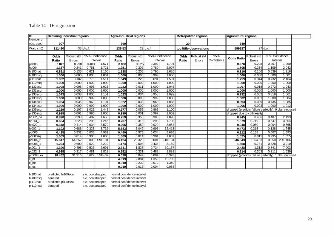
29

Table 14 - IE regression

IENumber of obs. used 907 799 20 649Wald chi2 311420 33 d.o.f. 136.53 29 d.o.f. 599287 27 d.o.f.

Odds Ratio

Robust std. Errors

Odds Ratio

Robust std. Errors

Odds Ratio

Robust std. Errors Odds Ratio Robust std.

Errorspe005 0.820 0.298 0.403 1.671 0.838 0.325 0.392 1.791 0.578 0.228 0.267 1.250hd004 1.137 0.241 0.751 1.721 1.251 0.302 0.780 2.007 1.505 0.234 1.109 2.042hi100hat 0.851 0.135 0.621 1.166 1.138 0.205 0.796 1.626 0.810 0.166 0.539 1.216hi100hsq 1.000 0.000 1.000 1.001 1.000 0.000 0.999 1.000 1.000 0.000 1.000 1.001pi110hat 1.082 0.182 0.775 1.511 1.049 0.220 0.691 1.591 1.259 0.344 0.732 2.164pi110hsq 1.000 0.000 1.000 1.000 1.000 0.000 1.000 1.000 1.000 0.000 1.000 1.000pi132ecu 1.008 0.008 0.993 1.023 1.022 0.011 1.000 1.045 1.007 0.018 0.972 1.043pi132esq 1.000 0.000 1.000 1.000 1.000 0.000 1.000 1.000 1.000 0.000 1.000 1.000pi133ecu 1.073 0.038 1.000 1.151 1.023 0.034 0.958 1.092 0.932 0.062 0.819 1.061pi133esq 1.000 0.000 0.999 1.000 1.000 0.000 0.999 1.000 1.002 0.001 1.000 1.004pi134ecu 1.034 0.035 0.969 1.104 1.022 0.033 0.960 1.088 0.893 0.089 0.735 1.085pi134esq 1.000 0.000 0.999 1.000 1.000 0.000 1.000 1.000 1.006 0.003 1.000 1.012pi135ecu 1.219 0.107 1.026 1.448 0.977 0.059 0.868 1.100 dropped (predicts failure perfectly): 9 obs. not usedpi135esq 0.998 0.001 0.996 1.000 0.999 0.001 0.997 1.002 dropped due to collinearityhf002_no 0.820 0.293 0.407 1.653 0.759 0.355 0.303 1.898 0.945 0.406 0.407 2.193hf013_2 0.604 0.223 0.293 1.246 0.707 0.318 0.293 1.708 1.579 0.719 0.647 3.854ha022_1 0.348 0.414 0.034 3.579 0.295 0.352 0.029 3.054 0.048 0.060 0.004 0.565hl002_1 1.102 0.686 0.325 3.732 5.683 5.049 0.996 32.418 0.473 0.315 0.128 1.745pd003 0.425 0.532 0.036 4.952 0.440 0.575 0.034 5.686 0.112 0.155 0.007 1.693pd003sq 1.009 0.014 0.983 1.036 1.009 0.014 0.981 1.037 1.025 0.015 0.995 1.055pd004_2 15.647 64.252 0.005 4.9E+04 6.124 26.320 0.001 2.8E+04 346.643 1564.53 0.050 2.4E+06pd005_1 1.294 0.600 0.522 3.210 1.174 0.593 0.436 3.159 1.568 0.731 0.628 3.910pt001_1 1.190 0.495 0.526 2.691 2.711 1.827 0.724 10.157 2.428 1.312 0.841 7.003pt022_3 0.935 0.317 0.481 1.818 0.952 0.331 0.482 1.881 0.714 0.303 0.311 1.639pm008_ex 18.452 31.916 0.622 5.5E+02 0.038 0.042 0.004 0.328 dropped (predicts failure perfectly): 1 obs. not usedc_nl 4.619 2.884 1.359 15.705c_be 0.310 0.232 0.072 1.340c_es 0.019 0.015 0.004 0.088

hi100hat predicted hi100ecu s.e. bootstrapped normal confidence intervalhi100hsq squared s.e. bootstrapped normal confidence intervalpi110hat predicted pi110ecu s.e. bootstrapped normal confidence intervalpi110hsq squared s.e. bootstrapped normal confidence interval

95% Confidence Interval

Declining Industrial regions Agro-Industrial regions Metropolitan regions Agricultural regions

too little observations

95% Confidence Interval

95% Confidence Interval

95% Confidence

30

7. Goodness of fit As already mentioned, understanding the link between the two classifications of labour status can help in reducing the dimension of (unexplained) measurement error to be taken into account when analysing transition flows using datasets that do not contain the desired classification. [2 repeated] ]1,0[ , )'(][ * ∈+==== jh

Ijhijhiiijh mzghljlpr αγα

Since we try to explain directly the (respondent) measurement error itself, the point is how ‘good’ are our estimates, i.e. how big are the residuals from our regressions. In a logit setting, there is no obvious measure of fit, differently from the linear case where the estimates are derived exactly through maximisation of a measure of fit. We propose a measure based on performing a simple ANOVA analysis on the predicted outcome of our regression, µi , on the dependent variable mi :

[6] ]))([(

]))()([(]var[)](var[

)var()var(

2

22

ii

ij

i

j

EEEEEE

totalbetweenR

µµµµ

µµ

µ −−

===

where µj , j = (0, 1) is the mean predicted probability µi for the two groups li = 0 and li = 1. This is different from Efron’s (1978) fit measure, where the sum of squared errors is related to the variance of the dependent variable:

[7] ]])[[(

])[(1 2

22

ii

iiEf lElE

lER−−−= µ

Compared with other measures proposed in the literature sharing the same approach (i.e. comparing the distribution of the predicted probability within the two success and failure groups), as that of Cramer (1999) we also provide24, the ANOVA has the advantage of allowing a simple interpretation in terms of percentage of explained variance. With reference to the figure below, Cramer index only compares µ 0 with µ 1 , the mean predicted probability for the two groups. The ANOVA index takes into consideration also the moment of degree 2 of the two distributions, and compares them with the variance of the overall distribution.

24 Cramer suggests to use λ = (average µ | mi = 1) - (average µ | mi = 0). Anova also compares average values in the two different outcome groups, but considers also the variance within those groups.

31

Figure 3 – measures of fit

Another classical measure of fit considers an arbitrary cut-off point, x*, and compares the number of well classified and wrongly classified observations. A cut-off point of 0.5 is often chosen. This is definitely inadequate in most cases, as the position and shape of the two distributions are not considered. We look for a cut-off point such that the sum of the frequency of wrongly classified observations within the two groups (Σ = A1 + A0) is minimised. This is a particular case of a more

general approach considering different weights for the two errors, where Σ = w1 A1 + w0 A0 is

minimised, with w0 + w1 = 1. We take this value Σ, which is confined in the range between 0 (perfect discrimination) and 1 (no discrimination), as another measure of fit. If we accept to make few (reasonable) assumptions on the shape of the distributions, the cut-off point that will minimise Σ would also equal A1 and A0. Results for the four group show acceptable results for the UI and IU groups, with a reduction in the overall variance of 35% and 23%, respectively. The Σ index25 is particularly good for the UI group, with a value as low as 0.31. This is coherent with the results from our regressions, where we found most variables to be significant. UE and IE group can very poorly be explained in terms of individual characteristics. While the reduction in the first two types of respondent measurement error is significant (although we can’t get any indication on the relative importance of respondent and interviewer measurement error from ECHP data), the reduction in the last two types of respondent measurement errors is negligible.

25 the shape of the Σ functions is showed in the Appendix.

0 µ0 x* µ1 1 f(Xb)

g (µj )

A1 A0

32

Table 15 – Measures of fit

R2(µ) Between Variance

Within Variance Cramer's λλλλ cut-off

point ΣΣΣΣ

UI 0.35 305.0 555.2 0.36 0.08 0.31

IU 0.23 60.0 198.0 0.23 0.22 0.52

UE 0.00 29.5 6,608.4 0.26 0.57 0.58

IE 0.01 28.6 2,291.5 0.12 0.81 0.69 8. Conclusions In this paper, we used ECHP data to investigate the effect of social, economical and institutional factors on labour status perception. We focused on those situations when the individual perception differs from the categorisation offered by the LFS (and imputed in the ECHP data), based on ILO definitions of employment, unemployment and participation to the labour force. We offered an explanation for the misperception, and described four main groups of ‘borderline’ individuals, the most interesting being those who declare to be unemployed while recorded as inactive, and those who declare to be inactive when recorded as unemployed. The first group is overemphasizing the job seeking efforts, while the second is underemphasizing them. ‘Victimisation’, i.e. considering society in general responsible for an individual’s current working situation, and the discouragement associated with it, is shown to be the main cause for being in this group. Such an attitude is (paradoxically) reinforced by assistance from the state itself, such that belonging to this group becomes ‘institutionalised’. These people do not compare in the unemployment statistics, but amount to an overall 35% of all (‘official’) unemployed workers in the European Union. This figure is around 30% in Italy, Germany, France, Ireland, reaching 50% and beyond in Portugal, Austria, Denmark and passing that of recorded unemployed in Belgium and the Netherlands. It is around 10% in Great Britain and Greece. These individuals are more or less dissatisfied as their ‘official’ counterparts, they vote, and thus would deserve the same attention as their more visible cousins. But bringing a little bit of hope and a little searching practice to them would increase the overall unemployment rate in the EU of as much as 3%! People underemphasizing their search efforts on the other side can normally rely on a family safety net (married women…), but their attitude is again reinforced by ‘institutional’ care. Also quite interesting are those part-time workers that declare to be either unemployed or inactive, since they could signal a positive attitude in dealing with their main status. All the evidence provided in this paper points to an inadequacy of labour statistics in keeping track of the complex reality of work and leisure time, an inadequacy that has a significant impact on the possibility of interregional comparisons of labour figures.

33

References

Bassi, Trivellato (1998), "Data and Modelling Strategies in estimating labour force gross flows affected by classification errors", Survey Methodology, 24

Byrne, D. and Strobl, E. (2001), Defining Unemployment in Developing Countries: The Case of Trinidad and Tobago, CREDIT Research Paper, No. 09, University of Nottingham.

Clark, K. and Summers, L. H. (1979). “Labor Market Dynamics and Unemployment: A Reconsideration”, Brookings Papers on Economic Activity, 1979: 1, pp. 13-60.

Cramer, J. (1999), Predictive Performance of the binary Logit model in Unbalanced Samples, Journal of the Royal Statistical Society, Series D (The Statistician), 48, pp. 85-94

Efron B. (1978), Regression and ANOVA with Zero-One Data: Measures of Residual Variation, Journal of the American Statistical Association, 73, pp. 113-212

Eurostat (2000), The European Community Household Panel, Waves 1-3, 1994-1996, European Commission

Eurostat (2001), ECHP Data Quality, European Commission, February

Eurostat (2001), ECHP UDB, Constuction of Variables, European Commission, May

Fisher, K., Fouarge, D., Muffels, R. and Verma V. (2000), Examining Flexible Labour in Europe. The first Three Waves of the ECHP, Institute for Social and Economic Research, University of Essex, Work and Organisation Research Centre, Faculty of Social and Behavioural Sciences and the Institute for Labour Studies (OSA), Tilburg University

Flinn, C. J. and Heckmann, J. J. (1983). “Are Unemployment and Out of the Labor Force Behaviourally Distinct Labor Market States?”, Journal of Labor Economics, 1, pp. 28-42.

Gonul, F. (1992). “New Evidence on Whether Unemployment and Out of the Labor Force are Distinct States”, Journal of Human Resources, 27, pp. 329-361.

Hausman, Abrevaya, Scott-Morton (1998), "Misclassification of the Dependent Variable in a Discrete-Response Setting", Journal of Econometrics, 87, pp. 239-269

Jones, S. R. G. and Riddell, W. C. (1999). “The Measurement of Unemployment: An Empirical Approach”, Econometrica, 67, pp. 147-162.

Kingdon, G. and Knight, J. (2000). “Are Searching and Non-Searching Unemployment Distinct States when Unemployment is High? The Case of South Africa”, The Centre of African Economies Working Paper Series, 2000/2.

Peracchi, F. (forthcoming) ”The European Community Household Panel Survey”, in W. Voges (ed.), Dynamic Approaches to Comparative Social Research, Avery Publishers, Aldershot.

34

Poterba, Summers (1995), "Unemployment Benefits and Labour Market Transitions: a Multinomial Logit Model with Errors in Classification", Review of Economics and Statistics, 77, pp. 207-216

Sorrentino, C. (2000). “International Unemployment Rates: How Comparable are They?”, Monthly

Labour Review, 2000, November, pp. 1-20. Veall M. & Zimmermann K. (1992), "Pseudo R2 in the Ordinal Probit Model", Journal of

Mathematical Sociology, 16, pp. 333-342

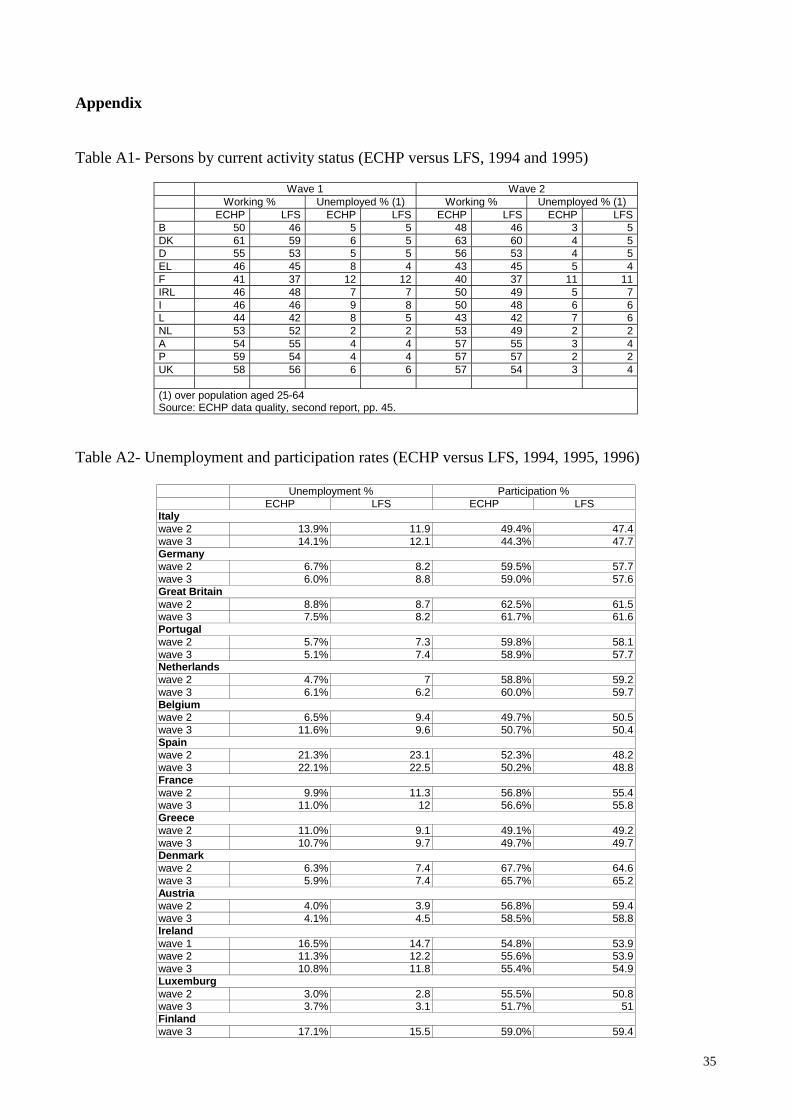
35

Appendix Table A1- Persons by current activity status (ECHP versus LFS, 1994 and 1995)

Wave 1 Wave 2 Working % Unemployed % (1) Working % Unemployed % (1)

ECHP LFS ECHP LFS ECHP LFS ECHP LFS B 50 46 5 5 48 46 3 5 DK 61 59 6 5 63 60 4 5 D 55 53 5 5 56 53 4 5 EL 46 45 8 4 43 45 5 4 F 41 37 12 12 40 37 11 11 IRL 46 48 7 7 50 49 5 7 I 46 46 9 8 50 48 6 6 L 44 42 8 5 43 42 7 6 NL 53 52 2 2 53 49 2 2 A 54 55 4 4 57 55 3 4 P 59 54 4 4 57 57 2 2 UK 58 56 6 6 57 54 3 4 (1) over population aged 25-64 Source: ECHP data quality, second report, pp. 45.

Table A2- Unemployment and participation rates (ECHP versus LFS, 1994, 1995, 1996)

Unemployment % Participation % ECHP LFS ECHP LFS

Italy wave 2 13.9% 11.9 49.4% 47.4 wave 3 14.1% 12.1 44.3% 47.7 Germany wave 2 6.7% 8.2 59.5% 57.7 wave 3 6.0% 8.8 59.0% 57.6 Great Britain wave 2 8.8% 8.7 62.5% 61.5 wave 3 7.5% 8.2 61.7% 61.6 Portugal wave 2 5.7% 7.3 59.8% 58.1 wave 3 5.1% 7.4 58.9% 57.7 Netherlands wave 2 4.7% 7 58.8% 59.2 wave 3 6.1% 6.2 60.0% 59.7 Belgium wave 2 6.5% 9.4 49.7% 50.5 wave 3 11.6% 9.6 50.7% 50.4 Spain wave 2 21.3% 23.1 52.3% 48.2 wave 3 22.1% 22.5 50.2% 48.8 France wave 2 9.9% 11.3 56.8% 55.4 wave 3 11.0% 12 56.6% 55.8 Greece wave 2 11.0% 9.1 49.1% 49.2 wave 3 10.7% 9.7 49.7% 49.7 Denmark wave 2 6.3% 7.4 67.7% 64.6 wave 3 5.9% 7.4 65.7% 65.2 Austria wave 2 4.0% 3.9 56.8% 59.4 wave 3 4.1% 4.5 58.5% 58.8 Ireland wave 1 16.5% 14.7 54.8% 53.9 wave 2 11.3% 12.2 55.6% 53.9 wave 3 10.8% 11.8 55.4% 54.9 Luxemburg wave 2 3.0% 2.8 55.5% 50.8 wave 3 3.7% 3.1 51.7% 51 Finland wave 3 17.1% 15.5 59.0% 59.4

36

Table A3 - LFS main activity during current year Codes Labels 1 normally working (working 15+ hours / week) 2 currently working (working less than 15 hours / week) 3 unemployed 4 discouraged worker 5 economically inactive -9 missing Source: ECHP – UDB, data dictionary and description of variables Table A4 - Variable construction rule

working at present at least 15 h/w or temporarily absent for some reason (vacation, sickness, bad weather, labour dispute, maternity leave…)

1

else any work in a job or business during the past 7 days, even if this was only for one or a few hours 2 else available to start within two weeks and active search to find a job 3 available to start within two weeks and received a job offer during past 4 weeks 3 available to start within two weeks and no active search because believe no suitable work available 4 available to start within two weeks and and no active search because already found work, to start in

future or awaiting outcome of application or interview 3

person has no job but is looking for a job

else 5 available to start within two weeks and no active search because engaged in other activity (study,

training, community or military service) 4

available to start within two weeks and no active search because and already found work, to start in future or awaiting outcome of application or interview

3

person has no job and is not looking for a job else 5

else -9 Source: ECHP Variable Construction Manual – European Commission Doc. Pan 167/01, adapted by the authors Please note that code 2 of LFS classification has a misleading label (“working less than 15 hours a week”). In facts, respondents are assigned code 2 if they declare not to have a regular job involving at least 15 hours a week, but to have done some kind of work in any job or business in the week prior to the interview. A more appropriate label would thus be “temporary or part-time work”. Around 3% of the code 2 people actually revealed to work for more than 15 hours per week.

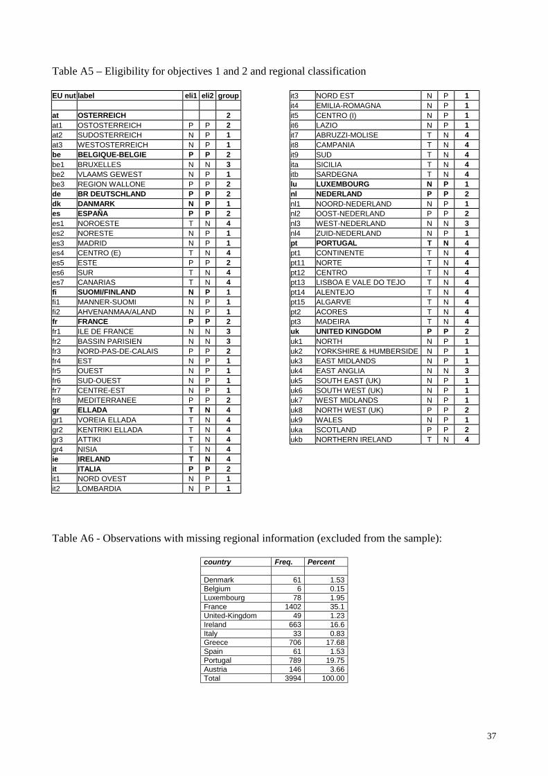
37

Table A5 – Eligibility for objectives 1 and 2 and regional classification EU nut label eli1 eli2 group at OSTERREICH 2 at1 OSTOSTERREICH P P 2 at2 SUDOSTERREICH N P 1 at3 WESTOSTERREICH N P 1 be BELGIQUE-BELGIE P P 2 be1 BRUXELLES N N 3 be2 VLAAMS GEWEST N P 1 be3 REGION WALLONE P P 2 de BR DEUTSCHLAND P P 2 dk DANMARK N P 1 es ESPAÑA P P 2 es1 NOROESTE T N 4 es2 NORESTE N P 1 es3 MADRID N P 1 es4 CENTRO (E) T N 4 es5 ESTE P P 2 es6 SUR T N 4 es7 CANARIAS T N 4 fi SUOMI/FINLAND N P 1 fi1 MANNER-SUOMI N P 1 fi2 AHVENANMAA/ALAND N P 1 fr FRANCE P P 2 fr1 ILE DE FRANCE N N 3 fr2 BASSIN PARISIEN N N 3 fr3 NORD-PAS-DE-CALAIS P P 2 fr4 EST N P 1 fr5 OUEST N P 1 fr6 SUD-OUEST N P 1 fr7 CENTRE-EST N P 1 fr8 MEDITERRANEE P P 2 gr ELLADA T N 4 gr1 VOREIA ELLADA T N 4 gr2 KENTRIKI ELLADA T N 4 gr3 ATTIKI T N 4 gr4 NISIA T N 4 ie IRELAND T N 4 it ITALIA P P 2 it1 NORD OVEST N P 1 it2 LOMBARDIA N P 1

it3 NORD EST N P 1 it4 EMILIA-ROMAGNA N P 1 it5 CENTRO (I) N P 1 it6 LAZIO N P 1 it7 ABRUZZI-MOLISE T N 4 it8 CAMPANIA T N 4 it9 SUD T N 4 ita SICILIA T N 4 itb SARDEGNA T N 4 lu LUXEMBOURG N P 1 nl NEDERLAND P P 2 nl1 NOORD-NEDERLAND N P 1 nl2 OOST-NEDERLAND P P 2 nl3 WEST-NEDERLAND N N 3 nl4 ZUID-NEDERLAND N P 1 pt PORTUGAL T N 4 pt1 CONTINENTE T N 4 pt11 NORTE T N 4 pt12 CENTRO T N 4 pt13 LISBOA E VALE DO TEJO T N 4 pt14 ALENTEJO T N 4 pt15 ALGARVE T N 4 pt2 ACORES T N 4 pt3 MADEIRA T N 4 uk UNITED KINGDOM P P 2 uk1 NORTH N P 1 uk2 YORKSHIRE & HUMBERSIDE N P 1 uk3 EAST MIDLANDS N P 1 uk4 EAST ANGLIA N N 3 uk5 SOUTH EAST (UK) N P 1 uk6 SOUTH WEST (UK) N P 1 uk7 WEST MIDLANDS N P 1 uk8 NORTH WEST (UK) P P 2 uk9 WALES N P 1 uka SCOTLAND P P 2 ukb NORTHERN IRELAND T N 4

Table A6 - Observations with missing regional information (excluded from the sample):

country Freq. Percent Denmark 61 1.53 Belgium 6 0.15 Luxembourg 78 1.95 France 1402 35.1 United-Kingdom 49 1.23 Ireland 663 16.6 Italy 33 0.83 Greece 706 17.68 Spain 61 1.53 Portugal 789 19.75 Austria 146 3.66 Total 3994 100.00

38

Table A7 - Auxiliary Income regressions

Tobit estimates Number of obs = 66283 LR chi2(8) = 1432.35 Prob > chi2 = 0 Log likelihood = -436386.6 Pseudo R2 = 0.0016 -------------------------------------------------------------------------------------------------------------------------------------------------------- hi100ecu Coef. Std.Err. t P>|t| [95% Conf. Interval] -------------------------------------------------------------------------------------------------------------------------------------------------------- pe005 0.687 0.077 8.958 0.000 0.537 0.837pe005sq -0.006 0.001 -4.899 0.000 -0.008 -0.004ha022_1 -1.809 1.989 -0.909 0.363 -5.707 2.090pd003 6.861 0.337 20.366 0.000 6.201 7.521pd003sq -0.077 0.004 -19.084 0.000 -0.085 -0.069pd004_2 12.304 1.445 8.518 0.000 9.473 15.135ph001 -24.954 0.890 -28.032 0.000 -26.699 -23.210pm008_ex 4.893 6.790 0.721 0.471 -8.415 18.202_cons 151.111 6.896 21.912 0.000 137.594 164.627-------------------------------------------------------------------------------------------------------------------------------------------------------- _se 179.865 0.496 (Ancillary parameter) -------------------------------------------------------------------------------------------------------------------------------------------------------- Obs. summary: 338 left-censored observations at hi100ecu<=0 65945 uncensored observations

Tobit estimates Number of obs = 66283 LR chi2(8) = 17146.43 Prob > chi2 = 0 Log likelihood = -356123.6 Pseudo R2 = 0.0235 -------------------------------------------------------------------------------------------------------------------------------------------------------- pi110ecu Coef. Std.Err. t P>|t| [95% Conf. Interval] -------------------------------------------------------------------------------------------------------------------------------------------------------- pe005 5.259 0.059 89.010 0.000 5.144 5.375pe005sq -0.044 0.001 -50.711 0.000 -0.046 -0.042ha022_1 5.273 1.363 3.867 0.000 2.600 7.945pd003 11.817 0.239 49.501 0.000 11.349 12.285pd003sq -0.127 0.003 -44.293 0.000 -0.133 -0.121pd004_2 -25.581 0.994 -25.736 0.000 -27.529 -23.633ph001 -13.989 0.617 -22.672 0.000 -15.198 -12.780pm008_ex 0.368 4.695 0.078 0.937 -8.834 9.571_cons -229.066 4.912 -46.635 0.000 -238.693 -219.438-------------------------------------------------------------------------------------------------------------------------------------------------------- _se 120.057 0.365 (Ancillary parameter) -------------------------------------------------------------------------------------------------------------------------------------------------------- Obs. summary: 10114 left-censored observations at pi110ecu<=0 56159 uncensored observations

39

Figure A1 – determination of Σ