ilovepdf.com split 3

3 Basic Thermal Design Theory forRecuperators

As defined in Chapter 1, in a recuperator, two fluids are separated by a heat transfersurface (wall), these fluids ideally do not mix, and there are no moving parts. In thischapter the thermal design theory of recuperators is presented. In a heat exchanger, when

hot and cold fluids are maintained at constant temperatures of Th andTc as shown in Fig.3.1a, the driving force for overall heat transfer in the exchanger, referred to as meantemperature difference (MTD), is simply Th � Tc. Such idealized constant temperatureson both sides may occur in idealized single-component condensation on one fluid side

and idealized single-component evaporation on the other fluid side of the exchanger.However, a number of heat transfer applications have condensation or evaporation ofsingle-component fluid on one side and single-phase fluid on the other side. In such cases,

the idealized temperature distribution is shown in Fig. 3.1b and c. The mean temperaturedifference for these cases is not simply the difference between the constant temperatureand the arithmetic mean of the variable temperature. It is more complicated, as will

be discussed. In reality, when the temperatures of both fluids are changing during theirpassage through the exchanger (see, e.g., Figs. 1.50, 1.52, 1.54, 1.56b, 1.57b, 1.60b, 1.63band 1.64b), the determination of the MTD is complex. Our objective in this chapter is to

conduct the appropriate heat transfer analysis in the exchanger for the evaluation ofMTD and/or performance. Subsequently, design methods are outlined and designproblems will be formulated.

The following are the contents of this chapter: An analogy between thermal, fluid, and

electrical parameters is presented in Section 3.1. Heat exchanger variables and the ther-mal circuit are presented in Section 3.2. The "-NTU method is introduced in Section 3.3.Specific "-NTU relationships for various flow arrangements are summarized in Section

3.4. The P-NTU method is introduced in Section 3.5, and P-NTU relationships forvarious flow arrangements are summarized in Section 3.6. The mean temperature differ-ence (MTD) method is introduced in Section 3.7. The MTD correction factors F for

various flow arrangements are presented in Section 3.8. It is shown in Section 3.9 that theresults of applications of "-NTU andMTDmethods are identical, although each methodhas some limitations. The -P and P1-P2 graphical presentation methods, which elim-

inate some of the limitations of the aforementioned methods, are presented in Section3.10. A brief description of various methods used to obtain "-NTU or P-NTU formulasfor various exchanger flow arrangements is presented in Section 3.11. Considering sevenvariables of the heat exchanger design problem, there are a total of 21 design problems

possible, as discussed in Section 3.12.

97Fundamentals of Heat Exchanger Design. Ramesh K. Shah and Dušan P. SekulicCopyright © 2003 John Wiley & Sons, Inc.

3.1 FORMAL ANALOGY BETWEEN THERMAL AND ELECTRICAL

ENTITIES

In heat exchanger analysis, a formal analogy between heat transfer and conduction of

electricity is very useful; to understand this analogy clearly, let us start with the defini-tions. Heat flow q is a consequence of thermal energy in transit by virtue of a temperaturedifference�T . By Ohm’s law, the electric current i is a consequence of electrical energy in

transit by virtue of an electromotive force (potential) difference �E. In both cases, therate of flow of related entity is inhibited by one or more recognizable resistances acting inseries and/or in parallel combinations.

Heat Flow ðHeat Transfer RateÞ Electric Current Flow

q ¼ �T

ðUAÞ�1¼ �T

R�T ¼ Rq i ¼ �E

R�E ¼ Ri ð3:1Þ

With this notion, the formal analogy between various parameters is presented in Table

3.1. It is important to note that the relationships between current, potential, resistance,conductance, capacitance, and time constant terms are analogous for these differentphysical processes. While the expressions for power and energy are analogous for heat

and current flow from the physics point of view, they are not analogous from the resis-tance circuit point of view as their formulas differ as shown in Table 3.1. Moreover, thereis no thermal analogy to electrical inductance or ‘‘inertia’’ in this analogy (not shown in

Table 3.1). Note that heat capacity or thermal capacitance energy storage terminologyused in heat transfer is used incorrectly as ‘‘thermal inertia’’ in the literature.

Since we know electrical circuit symbolism, we will find it convenient to borrow thesymbols for the thermal circuits used to describe the exchanger heat transfer process.

These are summarized in Fig. 3.2.We will also need an analogy between fluid flow in a pipe (exchanger) and electric

current for the pressure drop analysis of the exchanger. The basic parameters of pressure

drop (head), fluid flow rate, and flow losses are analogous to the voltage potential,

98 BASIC THERMAL DESIGN THEORY FOR RECUPERATORS

FIGURE 3.1 Idealized temperature distributions of one or both single-component phase-change

fluids: (a) one fluid condensing, the other evaporating; (b) one single-phase fluid cooling, the other

fluid evaporating; (c) one fluid condensing, the other single-phase fluid heating.

current, and resistance.y Since the flow losses are measured in terms of the pressure lossor head or fluid column, which have the same units as the potential, this analogy is not as

well defined as the analogy between heat transfer and electric current. Again, the rela-tionship between analogous parameters for fluid flow is not linear for transition andturbulent flows or developing laminar flows in pipes.

FORMAL ANALOGY BETWEEN THERMAL AND ELECTRICAL ENTITIES 99

TABLE 3.1 Analogies and Nonalogies between Thermal and Electrical Parameters

Parameter Electrical Thermal

Analogies

Current i ampere, A q W, Btu/hr

Potential E volts, V �T 8CðKÞ; 8Fð8RÞResistance R ohms, �; V/A R ¼ 1=UA 8C=W; 8F-hr/BtuConductance G siemens, S, A/V UA W/8C, Btu/hr-8FCapacitance C farads, F, A s/V �CC W � s=8C; Btu/8FTime constant RC s R �CC s, hr

Nonanalogies

Power iE W q W, Btu/hr

Energy

ð�

0iE d� J, W � s

ð�

0q d� J, Btu

FIGURE 3.2 Thermal circuit symbolism.

y Pipe and duct design based on one-dimensional lumped parameter analysis typically defines the flow resistance or

the flow loss coefficient K as equal to the number of velocity heads lost due to frictional effects [see Eq. (6. 53)].

3.2 HEAT EXCHANGER VARIABLES AND THERMAL CIRCUIT

In this section, starting with the assumptions built into heat exchanger design theory, thebasic problem for the exchanger heat transfer analysis is formulated. This includes the

differential equations used for the analysis as well as a list of independent and dependentvariables associated with heat exchanger design and analysis problems. Next, the basicdefinitions of important dimensional variables and important terminologies are intro-

duced. Finally, the thermal circuit, and expressions for UA and wall temperatures arepresented.

3.2.1 Assumptions for Heat Transfer Analysis

To analyze the exchanger heat transfer problem, a set of assumptions are introduced sothat the resulting theoretical models are simple enough for the analysis. The following

assumptions and/or idealizations are made for the exchanger heat transfer problemformulations: the energy balances, rate equations, boundary conditions, and subsequentanalysis [see, e.g., Eqs. (3.2) and (3.4) through (3.6) in differential or integral form].y

1. The heat exchanger operates under steady-state conditions [i.e., constant flowrates and fluid temperatures (at the inlet and within the exchanger) independentof time].

2. Heat losses to or from the surroundings are negligible (i.e. the heat exchangeroutside walls are adiabatic).

3. There are no thermal energy sources or sinks in the exchanger walls or fluids, suchas electric heating, chemical reaction, or nuclear processes.

4. The temperature of each fluid is uniform over every cross section in counterflow

and parallelflow exchangers (i.e., perfect transverse mixing and no temperaturegradient normal to the flow direction). Each fluid is considered mixed or unmixedfrom the temperature distribution viewpoint at every cross section in single-pass

crossflow exchangers, depending on the specifications. For a multipass exchan-ger, the foregoing statements apply to each pass depending on the basic flowarrangement of the passes; the fluid is considered mixed or unmixed betweenpasses as specified.

5. Wall thermal resistance is distributed uniformly in the entire exchanger.

6. Either there are no phase changes (condensation or vaporization) in the fluid

streams flowing through the exchanger or the phase change occurs under thefollowing condition. The phase change occurs at a constant temperature as fora single-component fluid at constant pressure; the effective specific heat cp;eff for

the phase-changing fluid is infinity in this case, and hence Cmax ¼ _mmcp;eff ! 1;where _mm is the fluid mass flow rate.

7. Longitudinal heat conduction in the fluids and in the wall is negligible.

8. The individual and overall heat transfer coefficients are constant (independent oftemperature, time, and position) throughout the exchanger, including the case ofphase-changing fluids in assumption 6.


y The complete set of differential equations and boundary conditions describing the mathematical models of heat

exchangers, based on these assumptions, is presented in Section 11.2.

9. The specific heat of each fluid is constant throughout the exchanger, so that theheat capacity rate on each side is treated as constant. Note that the other fluidproperties are not involved directly in the energy balance and rate equations, butare involved implicitly in NTU and are treated as constant.

10. For an extended surface exchanger, the overall extended surface efficiency �o isconsidered uniform and constant.

11. The heat transfer surface area A is distributed uniformly on each fluid side in asingle-pass or multipass exchanger. In a multipass unit, the heat transfer surfacearea is distributed uniformly in each pass, although different passes can have

different surface areas.

12. For a plate-baffled 1–n shell-and-tube exchanger, the temperature rise (or drop)per baffle pass (or compartment) is small compared to the total temperature rise

(or drop) of the shell fluid in the exchanger, so that the shell fluid can be treated asmixed at any cross section. This implies that the number of baffles is large in theexchanger.

13. The velocity and temperature at the entrance of the heat exchanger on each fluidside are uniform over the flow cross section. There is no gross flowmaldistributionat the inlet.

14. The fluid flow rate is uniformly distributed through the exchanger on each fluidside in each pass i.e., no passage-to-passage or viscosity-induced maldistributionoccurs in the exchanger core. Also, no flow stratification, flow bypassing, or flow

leakages occur in any stream. The flow condition is characterized by the bulk(or mean) velocity at any cross section.

Assumptions 1 through 5 are necessary in a theoretical analysis of steady-state

heat exchangers. Heat losses to the surroundings, if small, may be taken into accountapproximately by using the effective heat capacity rate Ceff for the hot fluid instead of theactual C ð¼ _mmcpÞ in the analysis. Ceff is determined based on the actual heat transfer rate

from the hot to cold fluid. Assumption 6 essentially restricts the analysis to single-phaseflow on both sides or one side with a dominating thermal resistance. For two-phase flowson both sides, many of the foregoing assumptions are not valid since mass transfer in

phase change results in variable properties and variable flow rates of each phase, and theheat transfer coefficients may also vary significantly. As a result, the "-NTU and othermethods presented in Sections 3.3 through 3.11 are not applicable to two-phase heat

exchangers. Assumptions 7 through 12 are relaxed in Chapter 4. Assumptions 13 and 14are addressed in Chapter 12.

If any of the foregoing assumptions are not valid for a particular exchanger applica-tion and the sections that cover the relaxation of these assumptions do not provide a

satisfactory solution, the approach recommended is to work directly with Eqs. (3.3) and(3.4), or a set of equations corresponding to the model. In this case, modify these differ-ential equations by including a particular effect, and integrate them numerically across

sufficiently small segments of the exchanger in which all the assumptions are valid. Referto Section 4.2.3.2 for an example.

In Sections 3.3 through 3.11, we present "-NTU, P-NTU, MTD, -P, and P1-P2

methods of exchanger heat transfer analysis for which the 14 assumptions are invoked.The corresponding model building, based on these assumptions, is discussed in detail inSection 11.2.

HEAT EXCHANGER VARIABLES AND THERMAL CIRCUIT 101

3.2.2 Problem Formulation

To perform the heat transfer analysis of an exchanger, our objective is to relate the heattransfer rate q, heat transfer surface area A, heat capacity rate C of each fluid, overallheat transfer coefficient U, and fluid terminal temperatures. Two basic relationships are

used for this purpose: (1) energy balance based on the first law of thermodynamics, and(2) rate equations for heat transfer, as outlined by Eqs. (2.1) and (2.2).

Consider a two-fluid exchanger (a counterflow exchanger as an example) shown in Fig

3.3 to arrive at the variables relating to the thermal performance of a two-fluid exchan-ger. Schematic of Fig. 3.3 and the balance equations for different exchanger flow arrange-ments may be different, but the basic concept of modeling remains the same. The analysisthat will follow is intended to introduce variables important for heat exchanger analysis.

Detailed approaches to a general thermodynamic problem formulation are presented inChapter 11.

Two differential energy conservation (or balance) equations (based on the energy

balance implied by the first law of thermodynamics) can be combined as follows forcontrol volumes associated with the differential element of dA area for steady-state flow,an overall adiabatic system, and negligible potential and kinetic energy changes:

dq ¼ q 00 dA ¼ �Ch dTh ¼ �Cc dTc ð3:2Þ


FIGURE 3.3 Nomenclature for heat exchanger variables (From Shah, 1983).

The negative signs in this equation are a result of Th and Tc decreasing with increasingA (these temperatures decrease with increasing flow length x as shown in Fig. 1.50);y also,dq is the heat transfer rate from the hot to cold fluid, C ¼ _mmcp is the heat capacity rate ofthe fluid, _mm is the fluid flow rate, cp is the fluid specific heat at constant pressure, T is the

fluid temperature, and the subscripts h and c denote hot and cold fluids, respectively. Theheat capacity rate C J/s � 8C (Btu/hr � 8F) is the amount of heat in joules (Btu) that mustbe added to or extracted from the fluid stream per second (hour) to change its tempera-

ture by 18C ð8FÞ. The product _mmcp ¼ C appears in the energy balance [Eq. (3.2)] forconstant cp, and hence C is commonly used in the heat exchanger analysis instead of _mmand cp as two parameters separately.

In general, for any isobaric change of state, Eq. (3.2) should be replaced by

dq ¼ � _mmh dhh ¼ � _mmc dhc ð3:3Þ

where h is the fluid specific enthalpy, J/kg (Btu/lbm). If the change of state is a phasechange, enthalpy differences should be replaced by enthalpies of phase change (either

enthalpy of evaporation or enthalpy of condensation). However, cp can be assumed asinfinity for condensing or evaporating single-component fluid streams. Hence, the phase-changing stream can be treated as a ‘‘single-phase’’ fluid having �T ¼ q=C or

dT ¼ dq=C, with C being infinity for a finite q or dq since the �T or dT ¼ 0 forisothermal condensing or evaporating fluid streams (see Fig. 3.1). Note that here�T ¼ Th;i � Th;o or Tc;o � Tc;i as appropriate.

The overall heat transfer rate equation on a differential base for the surface area dA of

Fig. 3.3 is

dq ¼ UðTh � TcÞlocal dA ¼ U�T dA ð3:4Þ

where U is the local overall heat transfer coefficient to be defined in Eq. (3.20).z Thus forthis differential element dA, the driving potential for heat transfer is the local temperaturedifference ðTh � TcÞ ¼ �T and the thermal conductance is UdA.

Integration of Eqs. (3.2) and (3.4) together over the entire heat exchanger surface forspecified inlet temperatures will result in an expression that will relate all important

operating variables and geometry parameters of the exchanger. The derivation of suchan expression for a counterflow exchanger will be presented in Section 3.3 together withfinal results for many industrially important exchanger flow arrangements. The common

assumptions invoked for the derivation and integration of Eqs. (3.2) and (3.4) aresummarized in Section 3.2.1.

Two basic equations, energy conservation (balance) and rate equations, could also be

written on an overall basis for the entire exchanger as follows (under the conditionsimplied by the above-mentioned idealizations):


y The sign convention adopted in Eq. (3.2) leads to positive value of heat transfer rate change along each dx

element, and should be considered only as formal (i.e., not necessarily in agreement with thermodynamic con-

vention for heat).z Note that although the overall heat transfer coefficient U is idealized as constant (see assumption 8 in Section

3.2.1), it can vary significantly in a heat exchanger. In that case, the mean overall heat transfer coefficient Um is

obtained from local U data (see Section 4.2.3). Even though U ¼ Um ¼ constant throughout this chapter, we

distinguish between U and Um in Sections 3.2.3 and 3.2.4 to emphasize how the theory is developed using U and

Um.

q ¼ð

C dT ¼ ChðTh;i � Th;oÞ ¼ CcðTc;o � Tc;iÞ ð3:5Þ

q ¼ð

U�T dA ¼ UmA�Tm ð3:6Þ

Here the subscripts i and o denote inlet and outlet, respectively;Th;o andTc;o represent the

outlet temperatures; they are bulk temperatures defined by Eq. (7.10) for a nonuniformtemperature distribution across a cross section; and Um and �Tm are the mean overallheat transfer coefficient and the exchanger mean temperature difference, respectively,and will be defined shortly.

From Eqs. (3.5) and (3.6) and Fig. 3.3, the steady-state overall-adiabatic heat exchan-ger behavior can thus be presented in terms of dependent fluid outlet temperatures orheat transfer rate as functions of four operating condition variables and three designer

controlled parameters:

Th;o;Tc;o or q|fflfflfflfflfflfflfflfflfflffl{zfflfflfflfflfflfflfflfflfflffl}

dependentvariables

¼ � ðTh;i;Tc;i;Ch;Cc|fflfflfflfflfflfflfflfflfflfflfflffl{zfflfflfflfflfflfflfflfflfflfflfflffl}

operating conditionvariables

U;A; flow arrangementÞ|fflfflfflfflfflfflfflfflfflfflfflfflfflfflfflfflfflfflfflfflfflffl{zfflfflfflfflfflfflfflfflfflfflfflfflfflfflfflfflfflfflfflfflfflffl}

parameters underdesigner’s control

|fflfflfflfflfflfflfflfflfflfflfflfflfflfflfflfflfflfflfflfflfflfflfflfflfflfflfflfflfflfflfflfflfflfflfflfflfflfflffl{zfflfflfflfflfflfflfflfflfflfflfflfflfflfflfflfflfflfflfflfflfflfflfflfflfflfflfflfflfflfflfflfflfflfflfflfflfflfflffl}

independent variables and parameters

ð3:7Þ

This equation represents a total of six independent and one or more dependent vari-

ables for a given heat exchanger flow arrangement. Of course, any one of the independentvariables/parameters in Eq. (3.7) can be made dependent (if unknown); in that case, oneof the three dependent variables in Eq. (3.7) becomes an independent variable/parameter.

Thus the most general heat exchanger design problem is to determine any two unknownvariables from this set when the rest of them are known.

For heat exchanger analysis, it is difficult to understand and work with such a large

number of variables and parameters as outlined in Eq. (3.7). From dimensional analysis,three dimensionless groups are formulated from six independent and one or more depen-dent variables of Eq. (3.7). The reduced number of nondimensional variables and para-meters simplifies much of the analysis, provides a clear understanding of performance

behavior, and the results can be presented in more compact graphical and tabular forms.The specific form of these groups is to some extent optional.

Five such options have been used, depending on which method of heat transfer

analysis has been used: the effectiveness–number of heat transfer units ("-NTU or P-NTU) method, the mean temperature difference (MTD) method, the nondimensionalmean temperature difference–temperature effectiveness ( -P) method, and the P1-P2

method. These methods are discussed in Sections 3.3 through 3.10.

3.2.3 Basic Definitions

The definitions of the mean overall heat transfer coefficient and mean temperaturedifference are introduced first.

The rate equation (3.4), after rearrangement, is presented in integral form as

ð

q

dq

�T¼

ð

AU dA ð3:8Þ


Now we define the mean temperature difference and mean overall heat transfercoefficient as follows using the terms in Eq. (3.8):

1

�Tm

¼ 1

q

ð

q

dq

�Tð3:9Þ

Um ¼ 1

A

ð

AU dA ð3:10Þ

Substitution of Eqs. (3.9) and (3.10) into Eq. (3.8) results into the following equationafter rearrangement:

q ¼ UmA�Tm ð3:11Þ

Here Um is the mean overall heat transfer coefficient, and �Tm is the true (or effective)

mean temperature difference (MTD), also referred to as mean temperature driving poten-tial or force for heat transfer.

Generally, the overall heat transfer coefficient is treated as constant in the heat exchan-

ger analysis. It is simply designated as U, without subscripts or overbars, throughout thebook except for Section 4.2, where various definitions of mean overall heat transfercoefficients are introduced. Thus the overall rate equation (3.6) is simply

q ¼ UA�Tm ð3:12Þ

Note that if U is treated as a constant, integration of Eq. (3.4) will yield

�Tm ¼ 1

A

ð

A�T dA ð3:13Þ

Other commonly used important entities for heat exchangers are the inlet temperaturedifference, temperature range, temperature approach, temperature pinch, temperaturegap, temperature meet, and temperature cross. They are discussed below and

summarized in Table 3.2.The inlet temperature difference (ITD) is the difference between inlet temperatures of

the hot and cold fluids and is designated as �Tmax in this book. �Tmax ¼ Th;i � Tc;i

is also sometimes referred to as the temperature span or temperature head in a heatexchanger.

The temperature range for a fluid is referred to as its actual temperature rise or drop

�T within the exchanger. The temperature ranges for hot and cold fluids in the exchan-gers are then �Th ¼ Th;i � Th;o and �Tc ¼ Tc;o � Tc;i, respectively.

The temperature approach for exchangers with single-phase fluids is defined as thedifference between outlet fluid temperatures ðTh;o � Tc;oÞ for all single-pass and multipass

flow arrangements except for the counterflow exchanger. For the latter, it is defined asthe smaller of ðTh;i � Tc;oÞ and ðTh;o � Tc;iÞ. The temperature approach for multiphasemulticomponent streams is defined as the minimum local temperature difference between

hot and cold fluid streams. This could occur anywhere in the exchanger, depending onthe flow arrangement, heat duty, and so on. It can be shown that the temperatureapproach for single-phase exchangers is related to the exchanger effectiveness " definedby Eq. (3.44) later as follows:


temperatureapproach ¼ ð1� "Þ�Tmax for a counterflow exchanger

½ð1� ð1þ C*Þ"��Tmax ¼ ðTh;o � Tc;oÞ for other exchangers

�

ð3:14Þ

where �Tmax ¼ Th;i � Tc;i and C* ¼ Cmin=Cmax. For some shell-and-tube, multipass,and two-phase exchangers, it may not be either easy or possible to determine quantita-tively the magnitude of the temperature approach. In that case, while the foregoing

definition is valid, it loses its usefulness.A temperature pinch refers to a local temperature difference within an exchanger (or

an array of exchangers) that is substantially less than either of two terminal temperature

differences and is minimum in the exchanger. In the limit, it can approach zero, which isreferred to as temperature meet defined below. The temperature pinch usually occurs inan exchanger with two-phase multicomponent fluids. In reality, a temperature pinchclose to zero will require a very large (approaching infinity) surface area for a single-

pass exchanger. Hence, for a finite-size heat exchanger, the exchanger would cease tofunction efficiently beyond the temperature pinch point (i.e., resulting in a more signifi-cant reduction in heat transfer than justified). However, for a multipass exchanger, the

temperature pinch could occur in one pass, and in that case, the performance of that passbeyond the temperature pinch is reduced significantly.

A temperature gap refers to the temperature difference between hot and cold fluid

outlet temperatures provided that Th;o > Tc;o:A temperature meet refers to the case when the temperature pinch is zero or the hot

and cold fluid temperatures are the same locally somewhere in the exchanger or at

outlets. This is an idealized condition and does not occur in a single-pass heat exchanger,but may occur in one of the passes of a multipass exchanger.

A temperature cross refers to the case when the cold fluid temperature becomes equalor greater than the hot fluid temperature within the exchanger. External temperature

cross refers to the case when the cold fluid outlet temperature Tc;o is greater than the hotfluid outlet temperature Th;o. There is no physical (actual) crossing of hot and cold fluidtemperature distributions within an exchanger. This is quite common in a counterflow

exchanger (see Fig. 1.50a) and other single-pass and multipass exchangers having high


TABLE 3.2 Expressions for Temperature Span, Range, Approach, Pinch, Gap, Meet, and Cross

Item Expression

Inlet temperature difference, ITD, maximim

temperature span or temperature head

Th;i � Tc;i

Temperature range for hot fluid Th;i � Th;o

Temperature range for cold fluid Tc;o � Tc;i

Temperature approach, counterflow exchanger min jðTh;i � Tc;oÞ; ðTh;o � Tc;iÞjTemoerature approach, all other exchangers Th;o � Tc;o

Temperature pinch at a local point in an exchanger Th � Tc with ðTh � TcÞ � ðTh;i � Tc;oÞor ðTh;o � Tc;iÞ

Temperature gap Th;o � Tc;o with Th;o > Tc;o

Temperature meet, counterflow sigle-phase exchanger Th;i ¼ Tc;o or Th;o ¼ Tc;i

Temperature meet, all other single-phase exchangers Th;o ¼ Tc;o

Temperature cross, single-pass exchangers Tc;o � Th;o with Tc;o > Th;o

Temperature cross, multipass exchangers Tc � Th with Tc > Th in one of the passes

NTUs (see Section 3.3.3 for the definition of NTU). The magnitude of the externaltemperature cross is Tc;o � Th;o. Internal temperature cross refers to the case when locallysomewhere within the exchanger Tc becomes equal to Th (within a pass or in a segment ofthe exchanger), and beyond that point along the flow length, Tc > Th in that pass or

segment; subsequently, reverse heat transfer takes place (original cold fluid transferringheat to the original hot fluid). The external temperature cross can occur with or withoutthe internal temperature cross; similarly an internal temperature cross can occur with or

without an external temperature cross (see Section 11.4.1).

3.2.4 Thermal Circuit and UA

To understand the exchanger overall heat transfer rate equation [Eq. (3.12)], consider thethermal circuit model of Fig. 3.4. Scale or fouling deposit layers are also shown on eachside of the wall.

In the steady state, heat is transferred from the hot fluid to the cold fluid by thefollowing processes: convection to the hot fluid wall, conduction through the wall, andsubsequent convection from the wall to the cold fluid. In many heat exchangers, a fouling

film is formed as a result of accumulation of scale or rust formation, deposits fromthe fluid, chemical reaction products between the fluid and the wall material, and/orbiological growth. This undesired fouling film usually has a low thermal conductivityand can increase the thermal resistance to heat flow from the hot fluid to the cold fluid.

This added thermal resistance on individual fluid sides for heat conduction through thefouling film is taken into account by a fouling factory rf ¼ 1=hf , where the subscript fdenotes fouling (or scale); it is shown in Fig. 3.4. Thus, the heat transfer rate per unit

area at any section dx (having surface areas dAh, dAc, etc.) can be presented by theappropriate convection and conduction rate equations as follows:

dq ¼ Th � Th; f

dRh

¼ Th; f � Tw;h

dRh; f

¼ Tw;h � Tw;c

dRw

¼ Tw;c � Tc; f

dRc; f

¼ Tc; f � Tc

dRc

ð3:15Þ

Alternatively

dq ¼ Th � Tc

dRo

¼ U dAðTh � TcÞ ð3:16Þ

where the overall differential thermal resistance dRo consists of component resistances inseries (similar to those shown in Fig. 3.4b for a heat exchanger):

1

U dA¼ dRo ¼ dRh þ dRh; f þ dRw þ dRc; f þ dRc ð3:17Þ

or

1

U dA¼ 1

ð�oh dAÞhþ 1

ð�ohf dAÞhþ dRw þ 1

ð�ohf dAÞcþ 1

ð�oh dAÞcð3:18Þ


y We also refer to the fouling factor as the unit fouling thermal resistance or concisely as fouling resistance

rf ¼ RRf ¼ 1=hf ¼ �f =kf where �f is the thickness of fouling layer and kf is the thermal conductivity of the fouling

material. Refer to Section 13.1 for more details on the fouling resistance concept.

Various symbols in this equation are defined after Eq. (3.24). If we idealize that the heattransfer surface area is distributed uniformly on each fluid side (see assumption 11 inSection 3.2.1), the ratio of differential area on each fluid side to the total area on the

respective side remains the same; that is,

dA

A¼ dAh

Ah

¼ dAc

Ac

¼ dAw

Aw

ð3:19Þ

Replacing differential areas of Eq. (3.18) by using corresponding terms of Eq. (3.19),

we get

1

UA¼ 1

ð�ohAÞhþ 1

ð�ohf AÞhþ Rw þ 1

ð�ohf AÞcþ 1

ð�ohAÞcð3:20Þ

It should be emphasized thatU and all h’s in this equation are assumed to be local. Usingthe overall rate equation [Eq. (3.6)], the total heat transfer rate will be

q ¼ UmA�Tm ¼ UmAðTh;e � Tc;eÞ ¼1

Ro

ðTh;e � Tc;eÞ ð3:21Þ


FIGURE 3.4 (a) Thermal resistances; (b) thermal circuit for a heat exchanger (From Shah, 1983).

and a counterpart of Eq. (3.15) for the entire exchanger is

q ¼ Th;e � Th; f

Rh

¼ Th; f � Tw;h

Rh; f

¼ Tw;h � Tw;c

Rw

¼ Tw;c � Tc; f

Rc; f

¼ Tc; f � Tc;e

Rc

ð3:22Þ

where the subscript e denotes the effective value for the exchanger, orðTh;e � Tc;eÞ ¼ �Tm. To be more precise, all individual temperatures in Eq. (3.22) should

also be mean or effective values for respective fluid sides. However, this additional sub-script is not included for simplicity. In Eq. (3.21), the overall thermal resistance Ro

consists of component resistances in series as shown in Fig. 3.4b.

1

UmA¼ Ro ¼ Rh þ Rh; f þ Rw þ Rc; f þ Rc ð3:23Þ

1

UmA¼ 1

ð�ohmAÞhþ 1

ð�ohm; f AÞhþ Rw þ 1

ð�ohm; f AÞcþ 1

ð�ohmAÞcð3:24Þ

For constant and uniform U and h’s throughout the exchanger, Eqs. (3.24) and (3.20)

are identical. In that case, Um ¼ U and we will use U throughout the book except forSection 4.2. In Eqs. (3.20) and (3.24), depending on the local or mean value, we define

Rh ¼ hot-fluid-side convection resistance ¼ 1

ð�ohAÞhor

1

ð�ohmAÞhRh; f ¼ hot-fluid-side fouling resistance ¼ 1

ð�ohf AÞhor

1

ð�ohm; f AÞhRw ¼ wall thermal resistance expressed by Eq: ð3:25Þ or ð3:26Þ

Rc; f ¼ cold-fluid-side fouling resistance ¼ 1

ð�ohf AÞcor

1

ð�ohm; f AÞc

Rc ¼ cold-fluid-side convection resistance ¼ 1

ð�ohAÞcor

1

ð�ohmAÞc

In the foregoing definitions, h is the heat transfer coefficient, discussed in detail in Section

7.1.4.3; hf is referred to as the fouling coefficient (inverse of fouling factor), discussed inChapter 13; A represents the total of primary and secondary (finned) surface area; and �ois the extended surface efficiency of an extended (fin) surface defined in Section 4.3.4. Inthe literature, 1=ð�ohÞf ¼ Rf A ¼ RRf is referred to as unit fouling resistance. Note that no

fins are shown in the upper sketch of Fig. 3.4; however, �o is included in the aforemen-tioned various resistance terms in order to make themmost general. For all prime surfaceexchangers (i.e., having no fins or extended surface), �o;h and �o;c are unity.

The wall thermal resistance Rw for flat walls is given by

Rw ¼

�wkwAw

for flat walls with a single layer wall

X

j

�wkwAw

� �

j

for flat walls with a multiple-layer wall

8

>>>><

>>>>:

ð3:25Þ


For a cylindrical (tubular) wall, it is given as

Rw ¼

lnðdo=diÞ2�kwLNt

for Nt circular tubes with a single-layer wall

1

2�LNt

X

j

lnðdjþ1=djÞkw; j

for Nt circular tubes with a multiple-layer wall

8

>>>><

>>>>:

ð3:26Þ

where �w is the wall plate thickness, Aw the total wall area of all flat walls for heatconduction, kw the thermal conductivity of the wall material, do and di the tube outside

and inside diameters, L the tube or exchanger length, and Nt the number of tubes. A flat(or plain) wall is generally associated with a plate-fin or an all-prime-surface plateexchanger. In this case,

Aw ¼ L1L2Np ð3:27Þ

Here L1, L2, and Np are the length, width, and total number of separating plates,respectively. The wall thickness �w is then the length for heat conduction.

If there is any contact or bond resistance present between the fin and tube or plate onthe hot or cold fluid side, it is included as an added thermal resistance on the right-handside of Eq. (3.23) or (3.24). For a heat pipe heat exchanger, additional thermal resistancesassociated with the heat pipe need to be included on the right-hand side of Eq. (3.23) or

(3.24); these resistances are evaporation resistance at the evaporator section of the heatpipe, viscous vapor flow resistance inside the heat pipe (very small), internal wick resis-tance at the condenser section of the heat pipe, and condensation resistance at the

condenser section.If one of the resistances on the right-hand side of Eq. (3.23) or (3.24) is significantly

higher than other resistances, it is referred to as the controlling resistance. It is considered

significantly dominant when it represents more than 80% of the total resistance. Forexample, if the cold side is gas (air) and the hot side is condensing steam, the thermalresistance on the gas side will be very high (since h for air is very low compared to that for

the condensing steam) and will be referred to as the controlling resistance for thatexchanger. However, for a water-to-water heat exchanger, none of the thermal resis-tances may be dominant if the water flow rates are about the same.

The lowest overall thermal resistance in a heat exchanger can be obtained by making

the hot- and cold-side thermal resistances about equal (considering wall and foulingresistances is negligible or low). Hence, a low h is often compensated by a high A tomake ð�ohAÞh � ð�ohAÞc. This is the reason the surface area on the gas side is about 5 to

10 times higher than that on the liquid-side when the liquid side heat transfer coefficient his 5 to 10 times higher than the h on the gas side. This would explain why fins are used onthe gas sides in a gas–to–liquid or gas–to–phase change exchanger.

In Eq. (3.24) or (3.12), the overall heat transfer coefficientUmay be defined optionallyin terms of the surface area of either the hot surface, the cold surface, or the wallconduction area. Thus,

UA ¼ UhAh ¼ UcAc ¼ UwAw ð3:28Þ


Thus in specifying UA as a product, we don’t need to specify A explicitly. However,the option of Ah, Ac, or Aw must be specified in evaluating U from the product UA sinceUh 6¼ Uc if Ah 6¼ Ac. It should be mentioned that the value of Ro ¼ 1=UA will always belarger than the largest thermal resistance component of Eq. (3.23). This means that UA

will always be smaller than the minimum thermal conductance component [a reciprocalof any one term of the right-hand side of Eq. (3.24)]. UA is referred to as the overallthermal conductance.

If the overall rate equation is based on a unit surface area

q

A¼ q 00 ¼ U�Tm ð3:29Þ

the unit overall thermal resistance is RRo ¼ 1=U. In this case, individual components ofresistances are also on a unit area basis, all based on either Ah or Ac explicitly as follows:

1

Uh

¼ 1

ð�ohÞhþ 1

ð�ohf Þhþ RwAh þ

Ah=Ac

ð�ohf Þcþ Ah=Ac

ð�ohÞc

¼ RRh þ1

�o;hRRh; f þ RRw

Ah

Aw

þ 1

�o;cRRc; f

Ah

Ac

þ RRc

Ah

Ac

ð3:30aÞ

1

Uc

¼ Ac=Ah

ð�ohÞhþ Ac=Ah

ð�ohf Þhþ RwAc þ

1

ð�ohf Þcþ 1

ð�ohÞc

¼ RRh

Ac

Ah

þ 1

�o;hRRh; f

Ac

Ah

þ RRw

Ac

Aw

þ 1

�o;cRRc; f þ RRc ð3:30bÞ

where 1=Uh is the unit overall thermal resistance based on the hot-fluid-side surface area.Similarly, 1=Uc is defined. Also RRj ¼ 1=ð�ohÞj , j ¼ h or c are unit thermal resistances for

hot or cold fluids, RRf ¼ 1=hf ¼ unit thermal fouling resistance, and RRw ¼ �w=kw ¼ unitwall thermal resistance. For a plain tubular exchanger, �o ¼ 1; then from Eq. (3.30), Uo

based on the tube outside surface area is given as follows after inserting the value of Rw

from the first equation of Eq. (3.26):

1

Uo

¼ 1

hoþ 1

ho; fþ do lnðdo=diÞ

2kwþ dohi; f di

þ dohidi

ð3:31aÞ

1

Ui

¼ dihodo

þ diho; f do

þ di lnðdo=diÞ2kw

þ 1

hi; fþ 1

hið3:31bÞ

Here the subscripts o and i denote the tube outside and inside, respectively; 1=Uo and

1=Ui are the unit overall thermal resistances based on the tube outside and inside surfacearea, respectively.

Knowledge of wall temperature in a heat exchanger is essential to determinethe localized hot spots, freeze points, thermal stresses, local fouling characteristics, or

boiling/condensing coefficients. In this case, Tw;h and Tw;c can be computed fromEq. (3.22) on a local basis as follows:

Th � Tw;h

Rh þ Rh; f

¼ Tw;c � Tc

Rc þ Rc; f

ð3:32Þ


Based on the thermal circuit of Fig. 3.4, when Rw is negligible, Tw;h ¼ Tw;c ¼ Tw, and Eq.(3.32) reduces to

Tw ¼ Th þ ½ðRh þ Rh; f Þ=ðRc þ Rc; f Þ�=Tc

1þ ½ðRh þ Rh; f Þ=ðRc þ Rc; f Þ�ð3:33Þ

When there is no fouling on either fluid side (Rh; f ¼ Rc; f ¼ 0Þ, this reduces further to

Tw ¼ ðTh=RhÞ þ ðTc=RcÞð1=RhÞ þ ð1=RcÞ

¼ ð�ohAÞhTh þ ð�ohAÞcTc

ð�ohAÞh þ ð�ohAÞcð3:34Þ

Equations (3.32) through (3.34) are also valid for the entire exchanger if all temperatures

are used as mean or effective values on respective fluid sides.

Example 3.1 In a shell-and-tube feedwater heater, cold water at 158C flowing at the rateof 180 kg/h is preheated to 908C by flue gases from 1508C flowing at the rate of 900 kg/h.The water flows inside the copper tubes ðdi ¼ 25mm, do ¼ 32mm) having thermalconductivity kw ¼ 381W=m �K. The heat transfer coefficients on gas and water sides

are 120 and 1200 W/m2 �K, respectively. The fouling factor on the water side is0.002m2 �K=W. Determine the flue gas outlet temperature, the overall heat transfercoefficient based on the outside tube diameter, and the true mean temperature difference

for heat transfer. Consider specific heats cp for flue gases and water as 1.05 and4:19 J=g �K respectively, and the total tube outside surface area as 5m2. There are nofins inside or outside the tubes, and there is no fouling on the gas side.

SOLUTION

Problem Data and Schematic: Fluid flow rates, inlet temperatures, and cold fluid outlettemperature are provided for a shell-and-tube exchanger of prescribed tube inner andouter diameters (Fig. E3.1). Also, the thermal conductivity of the tube and the thermalresistance on the cold fluid side are given. There are no fins on either side of the tubes.

Determine:Hot fluid outlet temperature Th;o, overall heat transfer coefficient U, and true

mean temperature difference �Tm.

Assumptions: The assumptions invoked in Section 3.2.1 are valid. Hot-fluid-side fouling

is negligible.


FIGURE E3.1

Analysis: The required heat transfer rate may be obtained from the overall energybalance for the cold fluid [Eq. (3.5)].

q ¼ CcðTc;o � Tc;iÞ ¼ ð _mmcpÞcðTc;o � Tc;iÞ

¼ 180 kg=h

3600 s=h

�

ð4:19 J=g �KÞð1000 g=kgÞð90� 15Þ8C ¼ 15,713W

�

Apply the same Eq. (3.5) on the hot fluid side to find the outlet temperature for flue gas:

Th;o ¼ Th;i �q

ð _mmcpÞh

Since

_mmh ¼900 kg=h

3600 s=h¼ 0:25 kg=s

cp;h ¼ ð1:05 J=g �KÞ � ð1000 g=kgÞ ¼ 1050 J=kg �K

we get

Th;o ¼ 1508C� 15,713W

0:25 kg=s� 1050 J=kg � 8C ¼ 90:18C Ans:

Since U is based on A ¼ Ah ¼ �doLNt, Eq. (3.31) reduces to the following form aftersubstituting the hot-fluid-side fouling factor (1=hf ) as zero, and replacing the subscripts oand i of U and h with h and c, respectively.

RR ¼ 1

Uh

¼ 1

hhþ 1

hh; fþ do lnðdo=diÞ

2kwþ dohc; f di

þ dohcdi

¼ 1

120W=m2 �Kþ 0:032m½lnð32mm=25mmÞ�2� 381W=m �K þ 0:002m2 �K=W� 0:032m

0:025m

þ 0:032m

120W=m2 �K� 0:025m

¼ ð0:00833þ 0:00001þ 0:00256þ 0:00107Þm2 �K=W ¼ 0:01197m2 �K=Wð69:6%Þ ð0:1%Þ ð21:4%Þ ð8:9%Þ

Hence,

Uh ¼ 83:54W=m2 �K Ans:

Note that the controlling thermal resistance for this feedwater heater is 69.6% on the flue

gas side. Now the mean temperature difference can be determined from Eq. (3.12) as

�Tm ¼ q

UhAh

¼ 15,713W

83:54W=m2 �K� 5m2¼ 37:68C Ans:


Discussion and Comments: Since the heat transfer coefficient on the cold side is greaterthan that on the hot side and the hot- and cold-side surface areas are about the same, thehot side becomes the controlling resistance side. This can be seen from the unit thermalresistance distribution as 69.6% of the total unit thermal resistance on the hot-gas side.

The tube wall, made of copper, turned out to be a very good conductor with very smallthermal resistance. Notice that the fouling resistance on the water side contributes aboutone-fifth (21.4%) of the total unit thermal resistance and hence about 21% surface area

penalty. If there had been no fouling on the water side, we would have reduced the heattransfer surface area requirement by about one-fifth. Hence, if it is desired to make asingle important improvement to reduce the surface area requirement in this exchanger,

the best way would be to employ fins on the gas side (i.e., employing low finned tubing inthe exchanger).

3.3 THE e-NTU METHOD

In the "-NTU method, the heat transfer rate from the hot fluid to the cold fluid in the

exchanger is expressed as

q ¼ "CminðTh;i � Tc;iÞ ¼ "Cmin �Tmax ð3:35Þ

where " is the heat exchanger effectiveness,y sometimes referred to in the literature as thethermal efficiency, Cmin is the minimum of Ch and Cc; �Tmax ¼ ðTh;i � Tc;iÞ is the fluidinlet temperature difference (ITD). The heat exchanger effectiveness " is nondimensional,

and it can be shown that in general it is dependent on the number of transfer units NTU,the heat capacity rate ratio C*, and the flow arrangement for a direct-transfer type heatexchanger:

" ¼ �ðNTU;C*; flow arrangementÞ ð3:36ÞHere the functional relationship � is dependent on the flow arrangement. The threenondimensional groups, ", NTU, and C* are first defined below. The relationshipamong them is illustrated next.

3.3.1 Heat Exchanger Effectiveness e

Effectiveness " is a measure of thermal performance of a heat exchanger. It is defined for

a given heat exchanger of any flow arrangement as a ratio of the actual heat transfer ratefrom the hot fluid to the cold fluid to the maximum possible heat transfer rate qmax

thermodynamically permitted:

" ¼ q

qmax

ð3:37Þ


y It should be emphasized that the term effectiveness may not be confused with efficiency. The use of the term

efficiency is generally restricted to (1) the efficiency of conversion of energy form A to energy form B, or (2) a

comparison of actual system performance to the ideal system performance, under comparable operating condi-

tions, from an energy point of view. Since we deal here with a component (heat exchanger) and there is no

conversion of different forms of energy in a heat exchanger (although the conversion between heat flow and

enthalpy change is present), the term effectiveness is used to designate the efficiency of a heat exchanger. The

consequence of the first law of thermodynamics is the energy balance, and hence the definition of the exchanger

effectiveness explicitly uses the first law of thermodynamics (see Chapter 11 for further discussion).

Here it is idealized that there are no flow leakages from one fluid to the other fluid, andvice versa. If there are flow leakages in the exchanger, q represents the total enthalpy gain(or loss) of the Cmin fluid corresponding to its actual flow rate in the outlet (and not inlet)stream. How do we determine qmax? It would be obtained in a ‘‘perfect’’ counterflow heat

exchanger (recuperator) of infinite surface area, zero longitudinal wall heat conduction,and zero flow leakages from one fluid to the other fluid, operating with fluid flow ratesand fluid inlet temperatures the same as those of the actual heat exchanger; also, assump-

tions 8 to 11, 13, and 14 of Section 3.2.1 are invoked for this perfect counterflowexchanger. This perfect exchanger is the ‘‘meterbar’’ (or ‘‘yardstick’’) used in measuringthe degree of perfection of actual exchanger performance. The value of " ranges from 0 to

1. Thus " is like an efficiency factor and has thermodynamic significance. As shownbelow, in such a perfect heat exchanger, the exit temperature of the fluid with the smallerheat capacity will reach the entering temperature of the larger heat capacity fluid.y

Consider a counterflow heat exchanger having infinite surface area. An overall energybalance for the two fluid streams is

q ¼ ChðTh;i � Th;oÞ ¼ CcðTc;o � Tc;iÞ ð3:38Þ

Based on this equation, for Ch < Cc, ðTh;i � Th;oÞ > ðTc;o � Tc;iÞ. The temperature drop

on the hot fluid side will thus be higher, and over the infinite flow length the hot fluidtemperature will approach the inlet temperature of the cold fluid as shown by the twobottom curves in Fig. 3.5, resulting in Th;o ¼ Tc;i. Thus for an infinite area counterflow

exchanger with Ch < Cc, we get qmax as

qmax ¼ ChðTh;i � Tc;iÞ ¼ Ch �Tmax ð3:39Þ

Similarly, for Ch ¼ Cc ¼ C;

qmax ¼ ChðTh;i � Tc;iÞ ¼ CcðTh;i � Tc;iÞ ¼ C�Tmax ð3:40Þ

Based on Eq. (3.38), for Ch > Cc, (Tc;o � Tc;iÞ > ðTh;i � Th;oÞ. Hence, Tc;o willapproach Th;i over the infinite length, and therefore

qmax ¼ CcðTh;i � Tc;iÞ ¼ Cc �Tmax ð3:41Þ

Or, more generally, based on Eqs. (3.39) throught (3.41),

qmax ¼ CminðTh;i � Tc;iÞ ¼ Cmin �Tmax ð3:42Þ

where

Cmin ¼Cc for Cc < Ch

Ch for Ch < Cc

(

ð3:43Þ

THE e-NTU METHOD 115

y It should be mentioned here that the second law of thermodynamics is involved implicitly in the definition of the

exchanger effectiveness since the ‘‘maximum possible heat transfer rate’’ is limited by the second law. Further

discussion of this and related issues is presented in Section 11.2.2.

Thus qmax is determined by Eq. (3.42) for defining the measure of the actual performanceof a heat exchanger having any flow arrangement. Notice that �Tmax ¼ Th;i � Tc;i inevery case and Cmin appears in the determination of qmax regardless of Ch > Cc or

Ch � Cc.Using the value of actual heat transfer rate q from the energy conservation equation

(3.5) and qmax from Eq. (3.42), the exchanger effectiveness " of Eq. (3.37) valid for all flow

arrangements of the two fluids is given by

" ¼ ChðTh;i � Th;oÞCminðTh;i � Tc;iÞ

¼ CcðTc;o � Tc;iÞCminðTh;i � Tc;iÞ

ð3:44Þ

Thus " can be determined directly from the operating temperatures and heat capacity

rates. It should be emphasized here that Th;o and Tc;o are the bulk outlet temperaturesdefined by Eq. (7.10). If there is flow and/or temperature maldistribution at the exchan-ger inlet, not only the fluid outlet temperatures but also the fluid inlet temperaturesshould be computed as bulk values and used in Eq. (3.44).

An alternative expression of " using q from the rate equation (3.12) and qmax from Eq.(3.42) is

" ¼ UA

Cmin

�Tm

�Tmax

ð3:45Þ

Now let us nondimensionalize Eq. (3.7). The mean fluid outlet temperatures Th;o andTc;o, the dependent variables of Eq. (3.7), are represented in a nondimensional form by

the exchanger effectiveness " of Eq. (3.44). There are a number of different ways to arrive


FIGURE 3.5 Temperature distributions in a counterflow exchanger of infinite surface area (From

Shah 1983).

at nondimensional groups on which this exchanger effectiveness will depend. Here weconsider an approach in which we list all possible nondimensional groups from visualinspection of Eqs. (3.44) and (3.45) as follows and then eliminate those that are notindependent; the exchanger effectiveness " is dependent on the following nondimensional

groups:

" ¼ �

�UA

Cmin

;Cmin

Cmax|fflfflfflfflfflfflfflfflffl{zfflfflfflfflfflfflfflfflffl}

independent

;Th;i � Th;o

�Tmax

;Tc;o � Tc;i

�Tmax

;�Tm

�Tmax

; flow arrangement

�

|fflfflfflfflfflfflfflfflfflfflfflfflfflfflfflfflfflfflfflfflfflfflfflfflfflfflfflfflfflfflfflfflfflfflfflfflfflfflfflfflfflfflfflfflfflfflfflfflffl{zfflfflfflfflfflfflfflfflfflfflfflfflfflfflfflfflfflfflfflfflfflfflfflfflfflfflfflfflfflfflfflfflfflfflfflfflfflfflfflfflfflfflfflfflfflfflfflfflffl}

dependent

ð3:46Þ

Note that �Tmax ¼ Th;i � Tc;i in the last three groups of Eq. (3.46) is an independentparameter. In Eq. (3.46), Cmax ¼ Cc for Cc > Ch and Cmax ¼ Ch for Ch > Cc, so that

Cmin

Cmax

¼

Cc

Ch

for Cc < Ch

Ch

Cc

for Ch < Cc

8

>>><

>>>:

ð3:47Þ

In order to show that the third through fifth groups on the right-hand side of Eq.(3.46) are dependent, using Eqs. (3.5) and (3.44), we can show that the first two of thethree groups are related as

Th;i � Th;o

�Tmax

¼ Cc

Ch

Tc;o � Tc;i

�Tmax

¼ "

Ch=Cmin

¼ " for Ch ¼ Cmin

"ðCmin=CmaxÞ for Ch ¼ Cmax

�

ð3:48Þ

and using Eq. (3.45), we can show that the fifth group of Eq. (3.46) is

�Tm

�Tmax

¼ "

UA=Cmin

ð3:49Þ

Since the right-hand side of the last equality of Eqs. (3.48) and (3.49) have ", Cmin=Cmax,and UA=Cmin as the only nondimensional groups and they are already included in Eq.(3.46), the dimensionless groups of the left-hand side of Eqs. (3.48) and (3.49) are depen-

dent. Thus Eq. (3.46) can be written in terms of nondimensional groups, without a loss ofgenerality, as follows:

" ¼ �UA

Cmin

;Cmin

Cmax

; flow arrangement

�

¼ �ðNTU;C*; flow arrangementÞ�

ð3:50Þ

where UA=Cmin (number of transfer units ¼ NTU) is a dimensionless parameter under

designer’s control, Cmin=Cmax (heat capacity rate ratio ¼ C*) is a dimensionless operatingparameter, and the heat exchanger flow arrangement built into � is also a designer’sparameter. Note that we could have obtained the three nondimensional groups, fromthe variables and parameters of Eq. (3.7), directly by using Buckingham’s � theorem

(McAdams, 1954) for a given flow arrangement. In Section 11.2, a rigorous modelingapproach is presented to determine the same dimensionless groups.

A comparison of Eqs. (3.50) and (3.7) will support the advantages claimed for

the nondimensional analysis approach. For each flow arrangement, we have reduced a


seven-parameter problemy [Eq. (3.7)], to a three-parameter problem, [Eq. (3.50)] for agiven heat exchanger flow arrangement of two fluids.

Before discussing the physical significance of the two independent parameters C* andNTU, let us introduce the definitions of the temperature effectiveness for the hot and cold

fluids. The temperature effectiveness "h of the hot fluid is defined as a ratio of thetemperature drop of the hot fluid to the fluid inlet temperature difference:

"h ¼Th;i � Th;o

Th;i � Tc;i

¼ �Th

�Tmax

ð3:51Þ

Similarly, the temperature effectiveness of the cold fluid is defined as a ratio of the

temperature rise of the cold fluid to the fluid inlet temperature difference:

"c ¼Tc;o � Tc;i

Th;i � Tc;i

¼ �Tc

�Tmax

ð3:52Þ

From an energy balance [Eq. (3.5)], and definitions of "h, and "c, it can be shown that

Ch"h ¼ Cc"c ð3:53Þ

A comparison of temperature effectivenesses with Eq. (3.44) for the exchanger (heattransfer) effectiveness reveals that they are related by

" ¼ Ch

Cmin

"h ¼"h for Ch ¼ Cmin

"h=C* for Ch ¼ Cmax

(

ð3:54Þ

" ¼ Cc

Cmax

"c ¼"c for Cc ¼ Cmin

"c=C* for Cc ¼ Cmax

(

ð3:55Þ

Now let us define and discuss C* and NTU.

3.3.2 Heat Capacity Rate Ratio C*

C* is simply a ratio of the smaller to larger heat capacity rate for the two fluid streams sothat C* � 1. A heat exchanger is considered balanced when C* ¼ 1:

C* ¼ Cmin

Cmax

¼ ð _mmcpÞmin

ð _mmcpÞmax

¼ðTc;o � Tc;iÞ=ðTh;i � Th;oÞ for Ch ¼ Cmin

ðTh;i � Th;oÞ=ðTc;o � Tc;iÞ for Cc ¼ Cmin

(

ð3:56Þ

C* is a heat exchanger operating parameter since it is dependent on mass flow ratesand/or temperatures of the fluids in the exchanger. The Cmax fluid experiences a

smaller temperature change than the temperature change for theCmin fluid in the absenceof extraneous heat losses, as can be found from the energy balance:

q ¼ Ch �Th ¼ Cc �Tc ð3:57Þ


y In counting, we have considered only one dependent variable of Eq. (3.7).

where the temperature ranges �Th and �Tc are

�Th ¼ Th;i � Th;o �Tc ¼ Tc;o � Tc;i ð3:58Þ

Let us reemphasize that for a condensing or evaporating fluid at ideally constant tem-perature, the �T range (rise or drop) is zero, and hence the heat capacity rate Capproaches infinity for a finite q ¼ C �T . Since C ¼ _mmcp, the effective specific heat of

condensing or evaporating fluid is hence infinity. TheC* ¼ 0 case then representsCmin asfinite and Cmax approaching infinity in the sense just discussed. The C* ¼ 0 case withCmin ¼ ð _mmcpÞmin ¼ 0 is not of practical importance, since _mm ¼ 0 in that case and hence

there is no flow on the Cmin side of the exchanger.

3.3.3 Number of Transfer Units NTU

The number of transfer unitsNTU is defined as a ratio of the overall thermal conductance

to the smaller heat capacity rate:

NTU ¼ UA

Cmin

¼ 1

Cmin

ð

AU dA ð3:59Þ

If U is not a constant, the definition of the second equality applies. NTU may also be

interpreted as the relative magnitude of the heat transfer rate compared to the rate ofenthalpy change of the smaller heat capacity rate fluid. A substitution of the UAmagnitude from Eq. (3.24) into Eq. (3.59) for U as constant results in

NTU ¼ 1

Cmin

1

1=ð�ohmAÞh þ Rh; f þ Rw þ Rc; f þ 1=ð�ohmAÞcð3:60Þ

NTU designates the nondimensional heat transfer size or thermal size of the exchanger,and therefore it is a design parameter. NTU provides a compound measure of the heat

exchanger size through the product of heat transfer surface area A and the overall heattransfer coefficient U. Hence, in general, NTU does not necessarily indicate the physicalsize of the exchanger. In contrast, the heat transfer surface area designates the physical

size of a heat exchanger. A large value of NTU does not necessarily mean that a heatexchanger is large in physical size. As a matter of fact, the automotive gas turbineregenerator at the idle operating point may have NTU � 10 and core volumeV � 0:01m3, whereas a chemical plant shell-and-tube exchanger may have NTU � 1

and V � 100m3. However, when comparing heat exchangers for a specific application,U=Cmin approximately remains constant; and in this case, a higher NTU value means aheat exchanger larger in physical size. Hence, NTU is sometimes also referred to as a heat

exchanger size factor. In general, higher NTU is obtained by increasing either U or A orboth or by decreasing Cmin. Whereas a change in Cmin affects NTU directly, a change inCmax (i.e., its flow rate) affects h on the Cmax side. This in turn influences U and NTU.

Thus, a change in the value of C* may have direct or indirect effect on NTU.NTU is also variously referred to as a performance factor or thermal length � in

the plate heat exchangery literature, and as reduced thermal flux in the shell-and-tube


y In a PHE with chevron plates, a plate with high chevron angle � has a high heat transfer coefficient and high

pressure drop in general and is referred to as a hard plate; in contrast, a soft plate has a low chevron angle � and low

heat transfer coefficient and low pressure drop in general.

exchanger literature. Other names are given in the following text with appropriate inter-pretations.

At low values of NTU, the exchanger effectiveness is low. With increasing values ofNTU, the exchanger effectiveness generally increases, and in the limit, it approaches a

thermodynamic asymptotic value. Note that the perfect exchanger requires thatNTU ! 1 (because A ! 1) for qmax ¼ Cmin �Tmax. The following approximate valuesof NTU will illustrate this point further.

Automobile radiator: NTU � 0:5 ! " � 40%

Steam plant condenser: NTU � 1 ! " � 63%

Regenerator for industrial gas turbine engine: NTU � 10 ! " � 90%

Regenerator for Stirling engine: NTU � 50 ! " � 98%

Regenerator for an LNG plant: NTU � 200 ! " � 99%

Another interpretation of NTU as nondimensional residence time is as follows bysubstituting Cmin ¼ �CCmin=�d in the definition of NTU:

NTU ¼ 1

ð1=UAÞCmin

¼ �dð1=UAÞ �CCmin

¼ �dRo

�CCmin

¼ �d* ð3:61Þ

Here Ro ¼ 1=UA is the overall thermal resistance; �CCmin ¼ ðMcpÞmin ¼ Cmin�d is the mini-mum-side fluid heat capacitance (M ¼ fluid mass in the exchanger at an instant of time)

in the exchanger at any instant of time; and �d is the dwell time, residence time, or transittime of a fluid particle passing through the exchanger. Thus, NTU can be interpreted as anondimensional residence time or a ratio of residence time to the time constant of the Cmin

fluid in the exchanger at an instant. NTU might well be expected to play an importantpart in the transient problem! And from the viewpoint of an observer riding with aparticle in the Cmin stream, he or she would indeed have a transient temperature–time

experience.Yet another interpretation of NTU is as follows. NTU is related to �Tm from Eq.

(3.45) with the use of Eq. (3.44) as

NTU ¼ �Tmax"

�Tm

¼ ðTh;i � Tc;iÞ"�Tm

¼ Ch �Th

Cmin �Tm

¼ Cc �Tc

Cmin �Tm

ð3:62Þ

Therefore, NTU is referred to as a temperature ratio (TR), where

NTU ¼

�Th

�Tm

¼ Th;i � Th;o

�Tm

for Ch ¼ Cmin

�Tc

�Tm

¼ Tc;o � Tc;i

�Tm

for Cc ¼ Cmin

8

>>><

>>>:

ð3:63Þ

Thus, NTU ¼ �Tmax;i=�Tm, where�Tmax;i is a maximum of�Th and�Tc. When�Tm

is equal to �Th or �Tc whichever is larger, NTU ¼ 1. Notice that Eq. (3.63) isconvenient for small values of NTU, in which case �Tm � Tm;h � Tm;c is a goodapproximation; there is no need to calculate �Tlm or F (see Section 3.7). Here Tm;h

and Tm;c are the arithmetic mean values of the corresponding terminal temperatures.


NTU is also directly related to the overall (total) Stanton number Sto formulated withU in place of h of Eq. (7.28) as

NTU ¼ Sto4L

Dh

ð3:64Þ

Thus, NTU can also be interpreted as a modified Stanton number. Note that here the

hydraulic diameter Dh is defined as follows depending on the type of heat exchangersurface geometry involved.

Dh ¼4� flow area

wetted perimeter¼ 4Ao

P¼ 4AoL

A

4� core flow volume

fluid contact surface area¼ 4pV

A¼ 4p

�¼ 4p

�

8

>>><

>>>:

ð3:65Þ

where p is the porosity, a ratio of void volume to total volume of concern. Here the firstdefinition of Dh is for constant cross-sectional flow passages in a heat exchanger.

However, when flow area is expanding/contracting across flow cross sections along theflow length as in three-dimensional flow passages (such as in a corrugated perforated fingeometry of Fig. 1.29f ), the more general second definition is applicable. In the second

definition, Dh ¼ 4p=� for plate-fin type and regenerative surfaces; for tube bundles andtube-fin surfaces, Dh ¼ 4p=�. Note that heat transfer and pressure drop Dh magnitudeswill be different if the heated and flow friction perimeters are different, as illustrated in thefootnote of p. 9.

Equations (3.63) and (3.59) may also be interpreted as the number of transfer unitsrequired by the heat duty ðNTU ¼ �Tmax;i=�TmÞ and the number of transfer unitsachieved by the heat exchanger ðNTU ¼ UA=CminÞ, respectively.

The foregoing definitions and interpretations are for the overall NTU for the exchan-ger. The number of heat transfer units individually on the hot and cold sides of theexchanger may be defined as:

ntuh ¼ð�ohAÞh

Ch

ntuc ¼ð�ohAÞc

Cc

ð3:66Þ

We use ntuh and ntuc in Chapter 9 when outlining the solution procedure for the sizingproblem for extended surface heat exchangers. The overall thermal resistance equation(3.24), in the absence of fouling resistances, can then be presented in terms of overall andindividual number of transfer units as

1

NTU¼ 1

ntuhðCh=CminÞþ RwCmin þ

1

ntucðCc=CminÞð3:67Þ

3.4 EFFECTIVENESS–NUMBER OF TRANSFER UNIT RELATIONSHIPS

In the preceding section we demonstrated that " is a function of NTU, C*, and flow

arrangement. We now derive this functional relationship for a single-pass counterflow

EFFECTIVENESS–NUMBER OF TRANSFER UNIT RELATIONSHIPS 121

exchanger and then summarize similar functional relationships for single-pass and multi-pass flow arrangements.

3.4.1 Single-Pass Exchangers

3.4.1.1 Counterflow Exchanger.y Consider a counterflow heat exchanger with the tem-perature distributions for hot and cold fluids as shown in Fig. 3.6. The fluid tempera-

tures on the left-hand end of the exchanger are denoted with the subscript I, and thoseon the other end with the subscript II.

In the analysis, we consider the overall counterflow exchanger as shown in Fig. 3.3

with only two passages. This is because the idealizations made in Section 3.2.1 (such asuniform velocities and temperatures at inlet, uniform surface area distribution, uniformU, etc.) are also invoked here. Thus, in fact, the hot-fluid passage shown represents all

hot-fluid flow passages, and the cold-flow passage shown consists of all cold-fluid flow


FIGURE 3.6 Counterflow heat exchanger with temperature distributions and differential

elements for energy balance and rate equation development.

y We derive the heat exchanger effectiveness in this section, and show how to obtain temperature distributions in

Chapter 11.

passages. This is the reason that Ch and Cc are associated with the respective single-flowpassages shown in Fig. 3.3 and not dCh and dCc.

Based on an energy balance consideration on the differential element dx,

dq ¼ �Ch dTh ¼ �Cc dTc ð3:68Þ

Here Th represents the bulk temperature of the hot fluid in the differential element dx of

Fig. 3.6. Tc is defined in a similar manner for the cold fluid.The rate equations applied individually to the dx length elements of the hot fluid, wall,

and the cold fluid yield

dq ¼

ð�ohAÞhðTh � Tw;hÞdx

Lfor the hot fluid ð3:69Þ

kw�w

Aw dx

LðTw;h � Tw;cÞ for the wall ð3:70Þ

ð�ohAÞcðTw;c � TcÞdx

Lfor the cold fluid ð3:71Þ

8

>>>>>>><

>>>>>>>:

Note that considering a general case, we have included the extended surface efficiency

�o in Eqs. (3.69) and (3.71), although fins are not shown in Fig. 3.6. After getting theexpressions for individual temperature differences from Eqs. (3.69)–(3.71), adding themup, and rearranging, we get

dq ¼ UAðTh � TcÞdx

Lð3:72Þ

Here U represents the local overall heat transfer coefficient for the element dA or dx.

However, we treat this local U the same as Um for the entire exchanger, and hence U willbe treated as a constant throughout the exchanger. Hence UA in Eq. (3.72) is given byEq. (3.20) or (3.24) without the fouling resistances on the hot and cold sides. If the fouling

or other resistances are present, UA in Eq. (3.72) will have those resistances included.Elimination of dq from Eqs. (3.68) and (3.72) will result in two ordinary differential

equations. We need two boundary conditions to solve them and they are

Thðx ¼ 0Þ ¼ Th;I Tcðx ¼ LÞ ¼ Tc;II ð3:73Þ

Now let us solve the set of Eqs. (3.68), (3.72), and (3.73) as follows to obtain a ratio of

terminal temperature differences so that we can determine the exchanger effectivenessdirectly. We derive the temperature distributions in Section 11.2.1. Here, effectively, wewill solve one differential equation that is based on the energy balance and rate equa-

tions. Substituting the values of dTh and dTc in terms of dq, Eq. (3.68) can be rearrangedto

dðTh � TcÞ ¼�

1

Cc

� 1

Ch

�

dq ð3:74Þ

Eliminating dq from Eqs. (3.72) and (3.74) and rearranging yields

dðTh � TcÞTh � Tc

¼ ��

1� Ch

Cc

�UA

Ch

dx

Lð3:75Þ


Integrating this equation from the hot-fluid inlet (section I) to the outlet section (sectionII) yields

Th;II � Tc;II

Th;I � Tc;I

¼ exp

�

�UA

Ch

�

1� Ch

Cc

��

ð3:76Þ

It can be shown algebraically that the left-hand side of Eq. (3.76) is

Th;II � Tc;II

Th;I � Tc;I

¼ 1� ðTh;I � Th IIÞ=ðTh;I � Tc;IIÞ1� ðTc;I � Tc IIÞ=ðTh;I � Tc;IIÞ

ð3:77Þ

Now employ the definitions of the temperature effectivenesses from Eqs. (3.51) and(3.52), using the nomenclature of Fig. 3.6:

"h ¼Th;I � Th ;II

Th;I � Tc;II

"c ¼Tc;I � Tc;II

Th;I � Tc;II

ð3:78Þ

Substituting the definitions of "h and "c in Eq. (3.77), it reduces to

Th;II � Tc;II

Th;I � Tc;I

¼ 1� "h1� "c

¼ 1� "h1� ðCh=CcÞ"h

ð3:79Þ

where Eq. (3.53) is used to obtain the last equality. Substituting Eq. (3.79) into (3.76) and

rearranging, we get

"h ¼1� exp½�ðUA=ChÞð1� Ch=CcÞ�

1� ðCh=CcÞ exp½�ðUA=ChÞð1� Ch=CcÞ�ð3:80Þ

Now the temperature effectiveness of the cold fluid, "c, can be determined eitherdirectly by employing its definition [Eq. (3.52)], or by substituting Eq. (3.80) into

(3.53). Using the second approach, gives us

"c ¼Ch

Cc

"h ¼1� exp½ðUA=CcÞð1� Cc=ChÞ�

ðCc=ChÞ � exp½ðUA=CcÞð1� Cc=ChÞ�ð3:81Þ

Notice that the argument of the exponential terms has been rearranged. By multiplyingboth numerator and denominator by exp f�ðUA=CcÞ½1� ðCc=ChÞ�g and rearranging, weget

"c ¼1� exp½�ðUA=CcÞð1� Cc=ChÞ�

1� ðCc=ChÞ exp½�ðUA=CcÞð1� Cc=ChÞ�ð3:82Þ

A comparison of Eqs. (3.80) and (3.82) reveals that Eq. (3.82) can be obtained directlyfrom Eq. (3.80) by replacing the subscripts h with c and c with h.

To generalize the solution, let Cmin ¼ Cc, C* ¼ Cc=Ch and NTU ¼UA=Cmin ¼ UA=Cc. In this case, " ¼ "c from Eq. (3.52), and Eq. (3.82) reduces to

" ¼ "cf ¼1� exp½�NTUð1� C*Þ�

1� C* exp½�NTUð1� C*Þ� ð3:83Þ


However, if Cmin ¼ Ch, then C* ¼ Ch=Cc, NTU ¼ UA=Cmin ¼ UA=Ch. In this case," ¼ "h from Eq. (3.51), and Eq. (3.80) reduces to the exchanger effectiveness expressionof Eq. (3.83). Thus, regardless of which fluid has the minimum heat capacity rate, the "-NTU expression for the counterflow exchanger is given by Eq. (3.83).

Two limiting cases of interest of Eq. (3.83) are C* ¼ 0 and 1. For the special caseof C* ¼ 0 (an evaporator or a condenser), the exchanger effectiveness ", Eq. (3.83),reduces to

" ¼ 1� expð�NTUÞ ð3:84Þ

Note that when C* ¼ 0, the temperature of the Cmax fluid remains constant throughoutthe exchanger, as shown in Fig. 3.1b and c. In this case, the Cmin fluid can have anyarbitrary flow arrangement. Hence Eq. (3.84) is valid for all flow arrangements when

C* ¼ 0.For the special case of C* ¼ 1, Eq. (3.83) reduces to the 0/0 form. Hence, using

l’Hospital’s rule (taking the derivatives of the numerator and the denominator separately

with respect to C* and substituting C* ¼ 1 in the resultant equation), we get

" ¼ NTU

1þNTUð3:85Þ

For all 0 < C* < 1; the value of " falls in between those of Eqs. (3.84) and (3.85), as

shown in Fig. 3.7.


FIGURE 3.7 Counterflow exchanger " as a function of NTU and C*.

By inverting Eq. (3.83), NTU for a counterflow exchanger can be expressed explicitlyas a function of " and C*:

NTU ¼ 1

1� C*ln

1� C*"

1� "ð3:86Þ

which for C* ¼ 0 and C* ¼ 1 (using l’Hospital’s rule) are given by

For C* ¼ 0 : NTU ¼ ln1

1� "or NTU ¼ ln

Th;i � Tc;i

Th;i � Tc;o

for Th;i ¼ constant

ð3:87Þ

For C* ¼ 1 : NTU ¼ "

1� "¼ Th;i � Th;o

Th;i � Tc;o

¼ Tc;o � Tc;i

Th;o � Tc;i

ð3:88Þ

The "-NTU results for the counterflow exchanger are presented in Fig. 3.7. The

following important observations may be made by reviewing Fig. 3.7:

1. The heat exchanger effectiveness " increases monotonically with increasing values

of NTU for a specified C*. For all C*, "! 1 as NTU ! 1. Note that this is truefor the counterflow exchanger, and " may not necessarily approach unity for manyother exchanger flow arrangements, as can be found from Tables 3.3 and 3.6.

2. The exchanger effectiveness " increases with decreasing values of C* for a specifiedNTU.

3. For "9 40%, the heat capacity rate ratio C* does not have a significant influence

on the exchanger effectiveness ". As a matter of fact, it can be shown that whenNTU ! 0, the effectiveness for all flow arrangements reduces to

" � NTU½1� 12NTUð1þ C*Þ� ð3:89Þ

This formula will yield highly accurate results for decreasing value of NTU for

NTU9 0.4.

4. Although not obvious from Fig. 3.7, but based on Eq. (3.84), the " vs. NTU curveis identical for all exchanger flow arrangements, including those of Tables 3.3 and

3.6 for C* ¼ 0.

5. Heat exchanger effectiveness increases with increasing NTU as noted above in item1, but at a diminishing rate. For example, increasing NTU from 0.5 to 1 at C* ¼ 1

increases " from 0.333 to 0.50; a 50% increase in " for a 100% increase in NTU (orapproximately 100% increase in surface area). Increasing NTU from 1 to 2 atC* ¼ 1 increases " from 0.50 to 0.667, a 33% increase in " for a 100% increase

in NTU (or size). Increasing NTU from 2 to 4 at C* ¼ 1 increases " from 0.667 to0.8, a 20% increase in " for a 100% increase in NTU (or size). This clearly shows adiminishing rate of increase in " with NTU.

6. Because of the asymptotic nature of the "-NTU curves, a significant increase inNTU and hence in the exchanger size is required for a small increase in " at highvalues of ". For example, for C* ¼ 1, " ¼ 90% at NTU ¼ 9, and " ¼ 92% at

NTU ¼ 11:5. Thus an increase of 2 percentage points in " requires an increase


of 28% in NTU and hence in the exchanger size for the same surface area andflow rates. Alternatively, a larger increase in NTU (or the size of the exchanger)is required to compensate for the same (or small) amount of heat loss to thesurroundings at high values of " in comparison to that for a lower " exchanger.

The counterflow exchanger has the highest exchanger effectiveness " for specified

NTU and C* of that for all other exchanger flow arrangements. Thus, for a givenNTU and C*, maximum heat transfer performance is achieved for counterflow; alter-natively, the heat transfer surface area is utilized most efficiently for counterflowcompared to all other flow arrangements.

Should we design heat exchangers at high effectiveness for maximum heat transfer?Let us interpret the results of Fig. 3.7 from the industrial point of view. It should beemphasized that many industrial heat exchangers are not counterflow, and the following

discussion in general is valid for other flow arrangements.When the heat exchanger cost is an important consideration, most heat exchangers

are designed in the approximate linear range of "-NTU curves (NTU � 2 or " � 60%,

such as in Fig. 3.7) that will meet the required heat duty with appropriate values of Cmin

and �Tmax. The reason for this is that an increase in the exchanger size (NTU) willincrease with " approximately linearly and hence will result in a ‘‘good’’ return on theinvestment of added surface area. However, when the exchanger is a component in

the system, and an increase in the exchanger effectiveness has a significant impact onreducing the system operating cost compared to an increase in the exchanger cost,the exchangers are designed for high effectivenesses. For example, a 1% increase in the

regenerator effectiveness approximately increases about 0.5% the thermal efficiency of anelectricity generating gas turbine power plant. This increase in the power plant efficiencywill translate into millions of dollars’ worth of additional electricity generated annually.

Hence, the cost of the regenerator represents only a small fraction of the annual savingsgenerated. Therefore, most gas turbine regenerators are designed at about " ¼ 90%. A1% increase in the effectiveness of a cryogenic heat exchanger used in an air separation

plant will decrease the compressor power consumption by about 5%. This will translateinto an annual savings of more than $500,000 (in 1995 dollars) in operating costs for a1000-ton oxygen plant. That is why most cryogenic heat exchangers are designed for" � 95%:

3.4.1.2 Exchangers with Other Flow Arrangements. The derivation of "-NTUformulas for other heat exchanger flow arrangements becomes more difficult as theflow arrangement becomes more complicated (Sekulic et al., 1999). The solutions

have been obtained in the recent past for many complicated flow arrangements, as inTable 3.6 and Shah and Pignotti (1989). Temperature distributions for counterflow,parallelflow, and unmixed–unmixed crossflow exchangers are derived in Sections 11.2.1

and 11.2.4.

"-NTU Results. Table 3.3 and Figs. 3.8 through 3.11 show the "-NTU formulas andresults for some heat exchanger flow arrangements. NTU can be expressed explicitly asa function of " and C* only for some flow arrangements and those formulas are

presented in Table 3.4. For all other flow arrangements, NTU is an implicit functionof " and C* and can be determined iteratively or by using appropriate analyticalmethods to solve the equation f (NTUÞ ¼ 0. C* cannot be expressed explicitly as a

function of " and NTU for any exchanger flow arrangements.


TABLE

3.3

e–NTU

Form

ulasandLim

itingValues

ofeforC*¼

1andNTU

!1

forVariousExchanger

FlowArrangem

ents

Flow

Arrangem

ent

"-NTU

Form

ulas

"-NTU

Form

ulas

forC*¼

1

AsymptoticValueof"

When

NTU

!1

Counterflow

"¼

1�exp½�

NTUð1

�C*Þ�

1�C*exp½�

NTUð1

�C*Þ�

"¼

NTU

1þNTU

"¼

1fopallC*

Parallelflow

"¼

1�exp½�

NTUð1

þC*Þ�

1þC*

"¼

1 2½1�expð�

NTUÞ�

"¼

1

1þC*

Crossflow,both

fluidsunmixed

"¼

1�expð�

NTUÞ

�exp½�

ð1þC*ÞN

TU�X

1 n¼1

C*nPnðN

TUÞ

PnðyÞ¼

1

ðnþ1Þ!X

n

j¼1

ðnþ1�jÞ

j!ynþj

Sameasgeneralform

ula

withC*¼

1

"¼

1forallC*

Crossflow,onefluid

mixed,

other

unmixed

ForC

minmixed,C

maxunmixed,

"¼

1�expf�

½1�expð�

NTU

�C*Þ�=

C*g

"¼

1�expf�

½1�expð�

NTUÞ�g

ForC

minmixed,

"¼

1�expð�

1=C*Þ

ForC

maxmixed,C

minunmixed,

"¼

1 C*ð1

�expf�

C*½1�expð�

NTUÞ�g

Þ

"¼

1�expf�

½1�expð�

NTUÞ�g

ForC

maxmixed,

"¼

½1�expð�

C*Þ�=

C*

Crossflow,both

fluidsmixed

"¼

1

1

1�expð�

NTUÞþ

C*

1�expð�

NTU

�C*Þ�

1

NTU

"¼

1

2=½1�expð�

NTUÞ��1=NTU

"¼

1

1þC*

1–2shell-and-tubeexchanger;

shellfluid

mixed;TEMA

Eshell

"¼

2

ð1þC*Þþ

ð1þC*2Þ1=

2cothð�=2Þ

where�¼

NTUð1

þC*2Þ1=

2

coth(�=2Þ¼

ð1þe�

�Þ=ð1

�e�

�Þ

"¼

2

2þ

ffiffiffi 2pcothð�=2Þ

where�¼

ffiffiffi 2pNTU

"¼

2

ð1þC*Þþ

ð1þC*2Þ1=

2

128


FIGURE 3.8 Parallelflow exchanger " as a function of NTU and C*.

FIGURE 3.9 Unmixed–unmixed crossflow exchanger " as a function of NTU and C*.


FIGURE 3.10 Unmixed–mixed crossflow exchanger " as a function of NTU and C*.

FIGURE 3.11 Mixed–mixed crossflow exchanger " as a function of NTU and C*.

From a review of Fig. 3.11, it is found for C* > 0 that the effectiveness of the mixed–mixed crossflow exchanger increases with increasing NTU up to some value of NTU

beyond which increasing NTU results in a decrease in ". The reason for this unexpectedbehavior is that due to the idealized complete mixing of both fluids, the hot-fluid tem-perature is lower than the cold-fluid temperature in a part of the exchanger, resulting in a

temperature cross (discussed in Section 3.6.1.2) and existence of entropy generationextrema (discussed in Section 11.4). Hence, heat transfer takes place in the reversedirection, which in turn reduces the exchanger effectiveness.

3.4.1.3 Interpretation of e-NTU Results. As noted in Eq. (3.7), the heat exchangerdesign problem in general has six independent and one or more dependent variables.

For analysis and concise presentation of the results, we arrived at a total of threedimensionless groups (", NTU, and C*) for this method. However, from the industrialviewpoint, the final objective in general is to determine dimensional variables and

parameters of interest in any heat exchanger problem. The nondimensionalization isthe shortest ‘‘road’’ to obtaining the results of interest. In this regard, let us review Eq.(3.35) again:

q ¼ "CminðTh;i � Tc;iÞ ¼ "ð _mmcpÞminðTh;i � Tc;iÞ ð3:90Þ

If we increase the flow rate on the Cc ¼ Cmin side (such as on the air side of a water-to-air

heat exchanger), it will increase C* ð¼ Cmin=CmaxÞ, reduce NTU ð¼ UA=CminÞ, and


TABLE 3.4 NTU as an Explicit Function of e and C* for Known Heat Exchanger Flow

Arrangements

Flow Arrangement Formula

Counterflow NTU ¼ 1

1� C*ln

1� C*"

1� "ðC* < 1Þ

NTU ¼ "

1� "ðC* ¼ 1Þ

Parallelflow NTU ¼ � ln½1� "ð1þ C*Þ�1þ C*

Crossflow (single pass)

Cmax (mixed), Cmin (unmixed) NTU ¼ �ln

�

1þ 1

C*lnð1� C*"Þ

�

Cmin (mixed), Cmax (unmixed) NTU ¼ � 1

C*ln½1þ C* lnð1� "Þ�

1–2 TEMA E Shell-and-Tube NTU ¼ 1

Dln

2� "ð1þ C*�DÞ2� "ð1þ C*þDÞ

where D ¼ ð1þ C*2Þ1=2

All exchangers with C* ¼ 0 NTU ¼ � lnð1� "Þ

hence will reduce " nonlinearly at a lower rate (see Figs. 3.7 to 3.11). Thus from Eq.(3.90), q will increase linearly with increasing Cmin and q will decrease nonlinearly at alower rate with decreasing ". The net effect will be that q will increase. From Eq. (3.5),

q ¼ CcðTc;o � Tc;iÞ ¼ ChðTh;i � Th;oÞ ð3:91Þ

Thus, overall, a lower increase in q and a linear increase in Cc will yield reduced

ðTc;o � Tc;iÞ; it means that Tc;o will be lower for a given Tc;i. Again from Eq. (3.91),Th;o will also be lower with increased q for given Ch and Th;i. These results are shownqualitatively by an arrow up or down in Table 3.5 depending on whether the particularvalue increases or decreases. It is interesting to note that both Th;o and Tc;o in this table

can either increase, decrease, or one increases and the other decreases! A thoroughunderstanding of the qualitative trends of the variables of this table is necessary tointerpret the experimental/analytical results and anomalies or unexpected test results.

Reviewing Eq. (3.90), the desired heat transfer rate q in a heat exchanger can beobtained by varying either " of Cmin since the ITD ð¼ Th;i � Tc;iÞ is generally a fixeddesign value in many applications. The effectiveness " can be varied by changing the

surface area A (the size of the exchanger) and hence NTU, impacting the capital cost; "increases with A or NTU nonlinearly and asymptotically. The minimum heat capacityrate Cmin ð¼ _mmcpÞ can be varied by changing the mass flow rate through a fluid pumpingdevice (fan, blower, or pump); the change inCmin has a direct (linear) impact on q. Hence,

in general, specified percentage change in Cmin will have more impact on q than thechange in " due to the same percentage change in A or the size of the exchanger.Current practice in many industries is to maintain the heat exchanger effectiveness

60% or lower to optimize the heat exchanger cost. The desired heat transfer rate isthen obtained by using a proper capacity fluid pumping device, which in turn has amajor impact on the operating cost. Thus the heat exchanger and the fluid pumping

device are selected individually. However, to get the desired heat transfer rate q in anexchanger, the better cost effective approach would be to select optimally the heatexchanger size (NTU) and the fluid pumping power to get the appropriate flow rate

(and hence CminÞ:Also, a review of Eq. (3.90) indicates that if there is an insufficient fluid flow rate _mm,

the exchanger will not provide the desired performance even if "! 100% for a given


TABLE 3.5 Effect of Increasing One Independent Variable at a Time on the Remaining Heat

Exchanger Variables Based on the e-NTU Relationshipsa

Specific Variable

with

Increasing Value

Variables Affected

" NTU C* q Th;o Tc;o

_mmh or Ch " " # " " "_mmc or Cc # # " " # #Th;i — — — " " "Tc;i — — — # " "hc or Ac " " — " # "hh or Ah " " — " # "a Cmin ¼ Cc for this table. ", increase; —, no change; #, decrease.

�Tmax. This is important when the fluid flow is blocked partially or totally in a heatexchanger, due to inadequate manufacturing or specific application/installation in asystem.

Equation (3.90) also implies that a perfectly designed exchanger may not operate

properly in a system if the heat duty of the exchanger is dictated by the system. Forexample, if the engine heat rejection is reduced due to the use of a smaller engine in agiven automobile, correspondingly, ðTh;i � Tc;iÞ will reduce for the same fan, and the

passenger compartment will not warm up to a comfortable level with the same auto-motive heater (i.e., given "). To be more specific, consider the coolant temperature Th;i

from the engine lower than the desired value (such as 758C vs. desired value of 908C) witha smaller engine. Hence, the ambient air will not be heated to the desired value (such as508C vs. the desired value of 628C) even though the heater is designed properly (i.e.,desired ") due to the reduced ITD.

3.4.1.4 Stream Symmetry. A two-fluid heat exchanger is considered to be streamsymmetric if the exchanger effectiveness " (or P) remains invariant by switching thetwo fluids (such as the tube fluid to the shell side, and the shell fluid to the tube side).Alternatively, the log-mean temperature difference correction factor F (defined in

Section 3.7.2) remains the same for the original and stream-switched configurations.Thus, for a stream symmetric exchanger, as shown in Eq. (3.36),

" ¼ � ðNTU;C*; flow arrangementÞ ð3:92Þ

regardless of whether the Cmin fluid is on the tube or shell side in a shell-and-tubeexchanger, for example.

All geometrically symmetrical exchangers are stream symmetric such as single-passcounterflow, parallelflow, and mixed–mixed and unmixed–unmixed crossflow exchan-gers. Some geometrically asymmetric exchangers (such as 1–2 and 1–1 TEMA E, 1–1

TEMA G, and 1–1 TEMA J exchangers, all with shell fluid mixed) are also streamsymmetric exchangers.

If an exchanger is stream asymmetric, the formula for the exchanger effectiveness " isdifferent for the two fluid sides of the exchanger (such as the shell side and tube side). Thismeans that

" ¼�1 ðNTU; C*; flow arrangementÞ for fluid 1 as Cmin fluid ð3:93aÞ�2 ðNTU; C*; flow arrangementÞ for fluid 2 as Cmin fluid ð3:93bÞ

(

where �1 and �2 are different functional relationships. Some examples of streamasymmetric exchangers are unmixed–mixed or mixed–unmixed crossflow, 1–2 TEMA

E with shell fluid unmixed, 1–n TEMA E (with 3 � n <1Þ with shell fluid mixed orunmixed, 1–2 TEMA G, 1–1 and 1–2 TEMA H, and 1–1, 1–2 and 1–4 TEMA Jexchangers with shell fluid mixed or unmixed. All heat exchanger arrays with parallelcoupling and those with compound coupling that include parallel coupling are stream

asymmetric.

Example 3.2 In an oil-to-water heat exchanger, the oil enters the exchanger at 1008Cwith a heat capacity rate of 3700W/K.Water is available at 158C and 0.6 kg/s. Determine

the exit temperatures in (a) counterflow, and (b) parallelflow arrangements for


U ¼ 500W/m2 �K and surface area of 10 m2. Consider cp ¼ 1:88 and 4.19 J/g �K for oiland water, respectively. If the ratio of convection thermal resistances of oil to water is 1.2,and the wall and fouling resistances are negligible, calculate the wall temperature at eachend of the counterflow and parallelflow exchangers.

SOLUTION

Problem Data and Schematic: Fluid flow rates, inlet temperatures, and overall heattransfer coefficient are provided for counterflow and parallelflow arrangements(Fig. E3.2A). Also, total heat transfer area and the ratio of thermal resistances of thetwo fluid sides are given.

Determine: Wall and fluid exit temperatures at each end ðx=L ¼ 0 and 1) of the counter-flow and parallelflow arrangements.

Assumptions: The assumptions invoked in Section 3.2.1 are valid, wall and fouling resis-tances and negligible, the ratio of thermal resistances of oil to water is uniform through-

out the exchanger.

Analysis: Knowing the inlet temperatures, we could use the definition of heat exchanger

effectiveness " to find the outlet temperatures of various exchangers. To determine ", weneed to determine C* and NTU. For the determination of C*, the heat capacity rates are

Ch ¼ 3700W=K

Cc ¼ ð _mmcpÞc ¼ 0:6 kg=s� ð4:19 J=g �K� 1000 g=kgÞ ¼ 2514W=K

where the subscripts h and c denote the hot (oil) and cold (water) sides, respectively.Hence, Cmin ¼ 2514W=K. Using the definitions of C* and NTU from Eqs. (3.56) and

(3.59), we have

C* ¼ Cc

Ch

¼ 2514W=K

3700W=K¼ 0:679

NTU ¼ UA

Cmin

¼ ð500W=m2 �KÞð10m2Þ2514W=K

¼ 1:989


FIGURE E3.2A

(a) Counterflow Exchanger: The exchanger effectiveness for the counterflow exchanger,from Eq. (3.83), is

" ¼ 1� exp½�NTUð1� C*Þ�1� C* exp½�NTUð1� C*Þ� ¼

1� exp½�1:989ð1� 0:679Þ�1� 0:679 exp½�1:989ð1� 0:679Þ� ¼ 0:736

Since water is the Cmin fluid, according to the definition of the effectiveness, Eq. (3.44),

" ¼ Tc;o � Tc;i

Th;i � Tc;i

¼ ðTc;o � 15Þ8Cð100� 15Þ8C ¼ 0:736

Hence,

Tc;o ¼ 158Cþ 0:736ð100� 15Þ8C ¼ 77:68C Ans:

Employing the energy balance equation (3.5), we could find the heat transfer rate onthe water side as

q ¼ CcðTc;o � Tc;iÞ ¼ ð2514W=KÞð77:6� 15Þ8C ¼ 157:4� 103 W

The oil outlet temperature from the energy balance equation (3.5) is then

Th;o ¼ Th;i �q

Ch

¼ 1008C� 157:4� 103 W

3700W=K¼ 57:58C Ans:

To determine the wall temperature at each end of the exchanger (designated by asecond subscript I and II), we use Eq. (3.34) with Rh; f and Rc; f ¼ 0, and Rh=Rc ¼ 1:2:

Tw;I ¼Th;i þ ðRh=RcÞTc;o

1þ ðRh=RcÞ¼ 1008Cþ 1:2� 77:68C

1þ 1:2¼ 87:88C Ans:

Tw;II ¼Th;o þ ðRh=RcÞTc;i

1þ ðRh=RcÞ¼ 57:58Cþ 1:2� 158C

1þ 1:2¼ 34:38C Ans:

(b) Parallelflow Exchanger: The heat exchanger effectiveness for a parallelflow exchan-ger, from Table 3.3, is

" ¼ 1� exp½�NTUð1þ C*Þ�1þ C*

¼ 1� exp½�1:989ð1þ 0:679Þ�1þ 0:679

¼ 0:574

The water outlet is then calculated from the definition of the effectiveness as

" ¼ Tc;o � Tc;i

Th;i � Tc;i

¼ ðTc;o � 15Þ8Cð100� 15Þ8C ¼ 0:574

so that

Tc;o ¼ 63:88C Ans:


The heat transfer rate on the water side is then

q ¼ CcðTc;o � Tc;iÞ ¼ ð2514W=KÞð63:8� 15Þ8C ¼ 122:7� 103 W

Subsequently, the oil outlet temperature is

Th;o ¼ Th;i �q

Ch

¼ 1008C� 122:7� 103 W

3700W=K¼ 66:88C Ans:

The wall temperature at each end of the exchanger is

Tw;I ¼Th;i þ ðRh=RcÞTc;i

1þ ðRh=RcÞ¼ 1008Cþ 1:2� 158C

1þ 1:2¼ 53:68C Ans:

Tw;II ¼Th;o þ ðRh=RcÞTc;o

1þ ðRh=RcÞ¼ 66:88Cþ 1:2� 63:88C

1þ 1:2¼ 65:28C Ans:

Discussion and Comments: In this problem, we have compared two thermodynamically

extreme performance exchangers (counterflow and parallelflow) at the same NTU, C*,and fluid inlet temperatures. The following observations may be made based on theresults presented graphically in Fig. E3.2B.

. The wall temperature across the exchanger length varies from 87.8 to 34.38C in thecounterflow exchanger and from 53.6 to 65.28C in the parallelflow exchanger. Thus

longitudinal wall temperature distribution is more uniform in the parallelflowexchanger compared to the counterflow exchanger.

. The lowest wall temperatures are 34.3 and 53.68C in the counterflow and parallel-

flow exchangers, respectively. Thus, the lowest wall temperature in the parallelflowexchanger is higher than that for the counterflow exchanger.

. Similarly, the highest wall temperature in the parallelflow exchanger is lower than

that for the counterflow exchanger (65.28C vs. 87.88C).


FIGURE E3.2B

It can be shown that these observations are true for comparing a parallelflow exchan-ger to an exchanger with any other flow arrangement for specified NTU, C*, and inlettemperatures.

As expected, the parallelflow exchanger provides lower heat transfer rate

ð78% ¼ 122:7 kW� 100=157:4 kWÞ than that of a counterflow exchanger. However, ifthe exchanger is designed for the effectiveness lower than 40%, there is not a significantdifference in the exchanger effectiveness and heat transfer rate between parallelflow and

counterflow exchangers at equal NTU and inlet temperatures. This is an industriallyimportant conclusion for low effectiveness waste heat recovery from exhaust gaseshaving SO2 as one of the constituents. The sulfuric acid condensation in a heat exchanger

can be prevented at atmospheric pressure if the minimum wall temperature is maintainedabove about 1508C. For this case, the parallelflow exchanger becomes an attractivesolution since its lowest wall temperature is higher than that of any other exchanger

flow arrangement.

Example 3.3 One important design point for a radiator design is to cool the engine at

50 km/h on a 7% grade road. Your responsibility as a design engineer is to make sure thatthe coolant (50% water–50% glycol) at the radiator inlet (top tank) does not exceed1208C temperature at 100 kPa gauge radiator cap pressure. Determine the radiator top

tank temperature for the following conditions: engine heat rejection rate q ¼ 35 kW,airflow rate 0.75 kg/s, air inlet temperature 538C, and water–glycol flow rate 1.4 kg/s.For this radiator, UA ¼ 1180W/K. The specific heats for the air and the water–glycol

mixture are 1009 and 3664 J/kg �K respectively. What will be the outlet temperature ofthe water–glycol mixture? Consider the radiator with both fluids unmixed.

SOLUTION

Problem Data and Schematic: Fluid flow rates, inlet temperature of the cold fluid, heat

transfer rate, and the total thermal conductance are given (see Fig. E3.3).

Determine: The inlet temperature of the hot fluid (water–glycol mixture).


FIGURE E3.3

Assumptions: The fluid properties and UA are constant, and the maximum inlettemperature for the hot fluid is 1208C at 100 kPa, beyond which it will boil in the engine.

Analysis: We could find the NTU from the information given. But first, we have to find

C* and Cmin:

Cair ¼ Cc ¼ ð _mmcpÞair ¼ 0:75 kg=s� 1009 J=kg �K ¼ 756:75W=K ¼ Cmin

Cliquid ¼ Ch ¼ ð _mmcpÞliquid ¼ 1:4 kg=s� 3664 J=kg �K ¼ 5129:6W=K

C* ¼ Cair

Cliquid

¼ 756:75W=K

5129:6W=K¼ 0:148

NTU ¼ UA

Cmin

¼ 1180W=K

756:75W=K¼ 1:559

From Fig. 3.9 or the Table 3.3 formula for an unmixed–unmixed crossflow exchanger, weget

" ¼ 0:769

Hence, Th;i from Eq. (3.35) is given by

Th;i ¼ Tc;i þq

"Cmin

¼ 538Cþ 35 kW� 1000W=kW

0:769� 756:75W=K¼ 113:18C Ans:

Since this is less than 1208C, the design is safe. If we would have determined Th;i > 1208C,we would have changed the radiator design (such as increasing A and hence UA andNTU) so that Th;i � 1208C.

Using the energy balance equation (3.5), we could find the water–glycol mixture outlettemperature as follows:

Th;o ¼ Th;i �q

Ch

¼ 113:18C� 35 kW� 1000W=kW

5129:6W=K¼ 106:38C Ans:

Discussion and Comments: As we discussed in Section 2.1.2.1, the two most importantheat exchanger design problems are the rating and sizing problems. However, based

on Eq. (3.7), the six independent variables of the problem for the specified flow arrange-ment yields a total of 21 different problems, summarized later in Table 3.11. Theproblem above is one example beyond the simple sizing problems (numbers 2 and 4 in

Table 3.11).In reality, one needs to design/size a radiator (i.e.,UA or NTU to be determined) such

that the top tank temperature does not exceed the boiling temperature of the water–glycol mixture at the worst design point (7% grade with air-conditioning on at the

highest blower speed for airflow in a desert summer condition); and at the same time,it requires ‘‘low’’ fan power to reduce the total cost of the radiator and fan as well as toreduce a negative impact on the fuel economy. However, to simplify the present problem,

the UA and airflow rate were given as part of the input data.


3.5 THE P-NTU METHOD

In the P-NTU method, the heat transfer rate from the hot fluid to the cold fluid in theexchanger is expressed as

q ¼ P1C1 �Tmax ¼ P2C2 �Tmax ð3:94Þ

where P is the temperature effectiveness for fluid 1 or 2, depending on the subscript 1 or 2,C ¼ _mmcp is the heat capacity rate for fluid 1 or 2 with the corresponding subscripts, andthe inlet temperature difference is �Tmax ¼ Th;i � Tc;i ¼ jT2;i � T1;ij. The temperatureeffectiveness P, similar to ", is nondimensional and is dependent on the number of

transfer units, heat capacity rate ratio, and the flow arrangement as will be shown inEq. (3.95). We define these dimensionless groups after providing the rationale for thismethod.

Historically, the P-NTU method has been used for designing shell-and-tube exchan-gers even before the "-NTU method became widely known in the 1940s. The "-NTUmethod represents a variant of the P-NTU method. Let us first discuss the reason for use

of the P-NTU method before presenting the details of the method.As shown in Table 3.3, the "-NTU relationship for a mixed–unmixed crossflow

exchanger is different depending on whether the mixed fluid is the Cmin or Cmax fluid,

because this exchanger is stream asymmetric, as discussed in Section 3.4.1.4. The otherstream asymmetric exchangers are also mentioned in Section 3.4.1.4. Hence, they willhave two "-NTU formulas, depending on which fluid side is the Cmin side. Consider thatthe heat capacity rate ratio (tube-to-shell) Ct=Cs ¼ 0:9 at an operating point in a 1–2

TEMAG exchanger. Now, due to a change in the process condition, the tube flow rate isincreased in the same exchanger, so that the new Ct=Cs ¼ 10=9 � 1:1. In this case,Ct ¼ Cmin for the first operating point, and Cs ¼ Cmin for the second operating point

in the same exchanger. One needs to use two different "-NTU formulas for the analysis ofthese two operating points resulting in two different "’s. Thus one has to keep track ofwhich is the Cmin fluid in the calculations.

To avoid possible errors and confusion, an alternative is to present the temperatureeffectiveness P of one fluid stream as a function of NTU based on that side’s heatcapacity rate and a ratio of heat capacity rates of that side to the other side, R. In thatcase, R can vary from 0 to1, and only one P-NTU formula will suffice for the complete

operating range of the exchanger. Of course, we will still have two different formulas(functional relationships as shown below for a stream asymmetric exchanger), and anyone will cover the complete operating range ð0 � R � 1Þ in the exchanger.

P1 ¼ �1 ðNTU1;R1; flow arrangementÞ P2 ¼ �2 ðNTU2;R2; flow arrangementÞð3:95Þ

Note that we use the general subscripts 1 and 2 in the P-NTUmethod for fluids 1 and 2 ofthe exchanger; and individual fluids 1 and 2 can be hot or cold, or Cmin or Cmax fluids.Somewhat arbitrarily, we choose the fluid 1 side as the shell fluid side regardless ofwhether it is the hot- or cold-fluid side in our representation here. For exchangers

other than shell-and-tube types, one of the two fluid sides is specifically designated asfluid 1 side, as shown in the corresponding sketches of Table 3.6.

It may not be a problem at all in a computer program to keep track of which fluid is

the Cmin before using the proper "-NTU formula for a stream asymmetric exchanger.

THE P-NTU METHOD 139

However, it may not be possible to determine whether a new but complicated flowarrangement of an industrial heat exchanger is stream symmetric or asymmetric.One does not need to know this fact if one uses the P-NTU method. The P-NTUformulas are flow arrangement dependent (as is the case for the "-NTU formulas), and

not on the dimensional value of Cs or Ct (or Cmin) as an additional variable in the "-NTUmethod. Thus, this is where the P-NTU method has an apparent advantage over the"-NTU method. Note that regardless of how complicated the exchanger flow arrange-

ment is, it may be possible now to obtain a closed-form P-NTU formula by the chainrule methodology (Pignotti and Shah, 1992; Sekulic et al., 1999). Now let us define P,NTU, and R of this method.

3.5.1 Temperature Effectiveness P

The temperature effectiveness P is referred to as thermal effectiveness in the shell-and-

tube heat exchanger literature. It is different for each fluid of a two-fluid exchanger. Forfluid 1, it is defined as the ratio of the temperature range (rise or drop) of fluid 1(regardless of whether it is a cold fluid or a hot fluid) to the inlet temperature difference(�Tmax or ITD) of the two fluids:

P1 ¼T1;o � T1;i

T2;i � T1;i

ð3:96Þ

Similarly, the temperature effectiveness of fluid 2 is defined as

P2 ¼T2;i � T2;o

T2;i � T1;i

ð3:97ÞIt can be shown that

P1 ¼ P2R2 P2 ¼ P1R1 ð3:98Þ

where R1 and R2 are defined later in Eqs. (3.105) and (3.106). Note that the temperatureeffectivenesses defined by Eqs. (3.96) and (3.97) are identical to those defined by Eqs.(3.51) and (3.52).

Comparing Eqs. (3.44) and (3.96), it is found that the temperature effectiveness P1 andthe exchanger effectiveness " are related as

P1 ¼Cmin

C1

" ¼ " for C1 ¼ Cmin

"C* for C1 ¼ Cmax

�

ð3:99ÞSimilarly,

P2 ¼Cmin

C2

" ¼ " for C2 ¼ Cmin

"C* for C2 ¼ Cmax

�

ð3:100Þ

Thus, the values of P1 and P2 will always be less than or equal to ".

3.5.2 Number of Transfer Units, NTU

The number of transfer units NTU1 and NTU2 are defined as

NTU1 ¼UA

C1

NTU2 ¼UA

C2

ð3:101Þ


It can be shown that

NTU1 ¼ NTU2R2 NTU2 ¼ NTU1R1 ð3:102Þ

These NTUi’s are related to NTU based on Cmin as

NTU1 ¼ NTUCmin

C1

¼NTU for C1 ¼ Cmin

NTU C* for C1 ¼ Cmax

(

ð3:103Þ

NTU2 ¼ NTUCmin

C2

¼NTU for C2 ¼ Cmin

NTU C* for C2 ¼ Cmax

(

ð3:104Þ

Thus, NTU1 or NTU2 is always less than or equal to NTU.

3.5.3 Heat Capacity Rate Ratio R

The heat capacity ratio R is defined as

R1 ¼C1

C2

¼ T2;i � T2;o

T1;o � T1;i

ð3:105Þ

R2 ¼C2

C1

¼ T1;o � T1;i

T2;i � T2;o

ð3:106Þ

and hence

R1 ¼1

R2

ð3:107Þ

Comparing Eqs. (3.105) and (3.106) with Eq. (3.56), we get

R1 ¼C1

C2

¼C* for C1 ¼ Cmin

1=C* for C1 ¼ Cmax

(

ð3:108Þ

R2 ¼C2

C1

¼C* forC2 ¼ Cmin

1=C* forC2 ¼ Cmax

(

ð3:109Þ

Thus R1 and R2 are always greater than or equal to C*. Individually, values of R1 and R2

range from 0 to 1, zero being for pure vapor condensation and infinity being for pureliquid vaporization.

3.5.4 General P-NTU Functional Relationship

Similar to the exchanger effectiveness ", the temperature effectiveness P1 is a function ofNTU1, R1 and flow arrangement represented by the function �1:

P1 ¼ �1 ðNTU1;R1; flow arrangementÞ ð3:110Þ

THE P-NTU METHOD 141

Similarly, P2 can be expressed as a function �2 of NTU2, R2, and flow arrangement.Hence the functions �1 and �2 will be dependent on the exchanger flow arrangement anddifferent for a stream asymmetric exchanger (i.e., the explicit formulas will be different).

The P-NTU results are generally presented on a semilog paper for the following

reason. The origin of the P-NTU method is related to shell-and-tube exchangers, andthe most useful NTU design range is from about 0.2 to 3.0 for shell-and-tube exchangers.Hence, the NTU scale is chosen as a logarithmic scale to stretch it in the range 0.2 to 3.0

to determine graphically a more accurate value of NTU, as was the case before thecomputer era.

3.6 P-NTU RELATIONSHIPS

As demonstrated in Section 3.5, P is a function of NTU,R and flow arrangement; here P,

NTU, and R should be defined consistently based on either fluid 1 or 2 side. Since thebasic energy balance and rate equations are identical to those mentioned while deriving a"-NTU relationship, we will not derive any specific P-NTU relationship here. Instead, we

illustrate the results for the 1–2 TEMA E exchanger with shell fluid mixed and discussthe concepts of temperature cross and multipassing to emphasize the peculiarity of someresults and how to obtain results for more complex flow arrangement. Explicit P-NTUformulas for a large number of exchanger flow arrangements are presented in Table 3.6.

It must be emphasized that all formulas are presented in Table 3.6 in terms of P1, NTU1

and R1 where fluid 1 is defined in the accompanying sketch in the first column on the left.If one needs an explicit formula for fluid 2, replace P1, NTU1, and R1 as P1 ¼ P2R2,

NTU1 ¼ NTU2R2 and R1 ¼ 1=R2 to obtain an explicit expression for P2 in terms ofNTU2 and R2.

3.6.1 Parallel Counterflow Exchanger, Shell Fluid Mixed, 1–2 TEMA E Shell

3.6.1.1 P-NTU Relationships. This exchanger has one shell pass and an even (rarely,odd) number of tube passes. The simplest arrangement is one shell pass and two tube

passes, simply referred to as a 1–2 exchanger. Such an exchanger, having two differentnozzle arrangements with respect to the tube return end, is shown in Fig. 3.12 withidealized temperature distributions. Note that the tube fluid in one pass is in the

counterflow direction and the tube fluid in the second pass is in the parallelflowdirection to the shell fluid flow direction.

Although this exchanger is not geometrically symmetric, it is highly stream symmetric

if the shell fluid is considered perfectly mixed at each cross section (see Section 3.4.1.4).Hence, the temperature effectiveness P is identical for the exchangers of Fig. 3.12a and bfor the same NTU and R. In other words, it does not make any difference in the theore-

tical P as to which end the exchanger inlet nozzle is located on. Also, the flow direction ofeither the tube or shell fluid or both fluids can be reversed, and P will still be the same forspecified values of NTU and R. Note that in all these cases, all four terminal tempera-tures and the tube fluid temperature at the end of the first tube pass, Tt;‘ will be identical,

as shown in Fig. 3.12a. The explicit P-NTU formula for this flow arrangement is given inTable 3.6, and the results are shown in Fig. 3.13. From this figure, it is clear that whenNTU1 ! 1 andR1 > 0, P1 is less than 1. Also note that P1 monotonically increases with

NTU1 to asymptotic values for all values of R1.


The P1-NTU1 relationship for the 1–n exchanger (one shell pass, even-n tube passeswith shell fluid mixed) is also presented in Table 3.6. Note that this 1–n exchanger ðn � 4Þis stream asymmetric. The temperature effectiveness P1 of the 1–n exchanger ðn > 2 andeven) is lower than that of the 1–2 exchanger for specified values of NTU1 and R1. The

maximum reduction in P1 of the 1–n exchanger over the 1–2 exchanger occurs at R1 ¼ 1.The thermal effectivenesses of the 1–n exchangers atR1 ¼ 1 are shown in Table 3.7. Froma review of this table, if the P1-NTU1 expression of Table 3.6 for the 1–2 exchanger is

used for the 1–n exchanger ðn � 4 and even), the error introduced is negligible for lowNTU1 (NTU1 < 3), particularly for R1 6¼ 1. However, if this error is not acceptable, it isrecommended to employ the P1-NTU1 expression [see Eq. (III.4) in Table 3.6] of the 1–4

exchanger for the 1–n exchanger for n � 4 and even. When n ! 1, the 1–n exchangereffectiveness approaches that of a crossflow exchanger with both fluids mixed, and theformula is given in Table 3.6 as Eq. (III.5).

The P-NTU results are presented in Figs. 3.14, 3.15, and 3.16 for 1–2 TEMA G, H,and J exchangers for comparisons with those in Fig. 3.13 for the 1–2 TEMAE exchanger.

3.6.1.2 Temperature Cross.y As defined earlier, the temperature cross refers to thesituation where the cold-fluid outlet temperature Tc;o is greater than the hot-fluid outlet

temperature Th;o; and in this case, the magnitude of the temperature cross isðTc;o � Th;oÞ. It derives its name from fictitious (e.g., counterflow exchanger; see Fig.1.50) or actual crossing (e.g., 1–2 TEMA E exchanger as shown in Fig. 3.17b) of thetemperature distributions of the hot and cold fluids in heat exchangers. Note that the

tube fluid temperature in the second pass beyond point X in Fig. 3.17b is higher thanthe shell fluid temperature at the corresponding axial position in the exchanger.

To further understand the temperature cross, consider a 1–2 exchanger with two

possible shell fluid directions with respect to the tube fluid direction as shown in Fig.3.17. Since the 1–2 exchanger is symmetric with respect to P or F, when the shell fluid isconsideredmixed, the same overall performance is obtained regardless of the direction of

the shell fluid or whether the hot or cold fluid is the shell fluid. In Fig. 3.17 the solid linetemperature distributions correspond to a high-NTUs case; and Ps and F are identical inboth cases for the same NTUs and Rs. Similarly, the dashed line temperature distribu-tions in Fig. 3.17 correspond to a low-NTUs case, and Ps and F will again be identical,

although different from those for the solid lines.The temperature distributions of Fig. 3.17b reveal that there is a temperature cross of

the shell fluid and the tube fluid in the second pass for the high-NTUs case. In region J of

this case, the second tube pass transfers heat to the shell fluid. This is contrary to theoriginal design, in which ideally, heat transfer should have taken place only in onedirection (from the shell fluid to the tube fluid in Fig. 3.17) throughout the two passes.

This temperature cross can be explained qualitatively as follows: Although an additionof surface area (a high value of NTUs or a low value of F) is effective in raising thetemperature Tt;‘ of the tube fluid at the end of the first tube pass, the temperature of the

tube fluid rises in the second tube pass up to a point X. Beyond this point, the tempera-ture of the shell fluid is lower than that of the tube fluid, since we have considered theshell fluid mixed at a cross section and it is cooled rapidly by the first tube pass. Thus the

P-NTU RELATIONSHIPS 143

y In all the discussion of this subsection, we consider only the external temperature cross; refer to Section 11.4.1 for

external and internal temperature crosses. Also, throughout this subsection, the shell fluid is considered hot, the

tube fluid cold, and heat transfer takes place from the shell fluid to the tube fluid. However, all the discussion and

results presented in this subsection are valid if the shell fluid is cold and the tube fluid is hot.

TABLE

3.6

P1–NTU

1Form

ulasandLim

itingValues

ofP1forR

1¼

1andNTU

1!

1forVariousExchanger

FlowArrangem

ents

Flow

Arrangem

enta

Eq.No.

GeneralForm

ula

bValueforR

1¼

1c

ValueforNTU

1!

1

I.1.1

P1¼

1�exp½�

NTU

1ð1

�R

1Þ�

1�R

1exp½�

NTU

1ð1

�R

1Þ�

P1¼

NTU

1

1þNTU

1

P1!

1forR

1�

1

P1!

1=R

1forR

1�

1

I.1.2

NTU

1¼

1

1�R

1

ln1�R

1P1

1�P1

NTU

1¼

P1

1�P1

NTU

1!

1Counterflow

exchanger,stream

symmetric

I.1.3

F¼

1F¼

1F¼

1

I.2.1

P1¼

1�exp½�

NTU

1ð1

þR

1Þ�

1þR

1

P1¼

1 2½1�expð�

2NTU

1Þ�

P1!

1

1þR

1

I.2.2

NTU

1¼

1

1þR

1

ln1

1�P1ð1

þR

1Þ

NTU

1¼

1 2ln

1

1�2P1

NTU

1!

1Parallelflow

exchanger,stream

symmetric

I.2.3

F¼

ðR1þ1Þln½ð1

�R

1P1Þ=ð1

�P1Þ�

ðR1�1Þln

½1�P1ð1

þR

1Þ�

F¼

2P1

ðP1�1Þln

ð1�2P1Þ

F!

0

Single-pass

crossflow

exchanger,both

fluidsunmixed,stream

symmetric

II.1

P1¼

1�expð�

NTU

1Þ

�exp½�

ð1þR

1ÞN

TU

1�

�X1 n¼1

1

ðnþ1Þ!R

n 1

�Xn

j¼1

ðnþ1�jÞ

j!ðN

TU

jÞnþj

SameasEq.(II.1)

withR

1¼

1

P1!

1forR

1�

1

P1!

1 R1

forR

1�

1

P1�

1�exp

�NTU

0:22

1

R1

ðe�R1NTU

0:78

1�1Þ�

Thisapproxim

ate

equationisaccurate

within

1%

for

1<

NTU

1<

7:

144

II.2.1

P1¼

1�expð�

KR

1Þ

R1

P1¼

1�expð�

KÞ

P1!

1�expð�

R1Þ

R1

K¼

1�expð�

NTU

1Þ

K¼

1�expð�

NTU

1Þ

II.2.2

NTU

1¼

ln1

1þð1=R

1Þln

ð1�R

1P1Þ

NTU

1¼

ln1

1þlnð1

�P1Þ

NTU

1!

1

Single-pass

crossflow

exchanger,

fluid

1unmixed,fluid

2mixed

II.2.3

F¼

ln½ð1

�R

1P1Þ=ð1

�P1Þ�

ðR1�1Þln

½1þð1=R

1Þln

ð1�R

1P1Þ�

F¼

P1

ðP1�1Þln

½1þlnð1

�P1Þ�

F!

0

II.3.1

P¼

1�exp

�

�K R1

�

K¼

1�expð�

R1�N

TU

1Þ

P¼

1�expð�

KÞ

K¼

1�expð�

NTU

1Þ

P1!

1�exp

�

�1 R1

�

II.3.2

NTU

1¼

1 R1

ln

�1

1þR

1lnð1

�P1Þ�

NTU

1¼

ln1

1þlnð1

�P1Þ

NTU

1!

1

Single-pass

crossflow

exchanger,

fluid

1mixed,fluid

2unmixed

II.3.3

F¼

lnð1

�R

1P1Þ=ð1

�P1Þ�

ð1�1=R

1Þln½1þR

1lnð1

�P1Þ�

F¼

P1

ðP1�1Þln½1þlnð1

�P1Þ�

F!

0

II.4

P1¼

�1 K1

þR

1

K2

�1

NTU

1

��1

P1¼

�2 K1

�1

NTU

1

��1

P1!

1

1þR

1

K1¼

1�expð�

NTU

1Þ

K2¼

1�expð�

R1�N

TU

1Þ

Single-pass

crossflow

exchanger,both

fluidsmixed,stream

symmetric

(continued

over)

145

TABLE

3.6

(Continued)

Flow

Arrangem

enta

Eq.No.

GeneralForm

ula

bValueforR

1¼

1c

ValueforNTU

1!

1

III.1.1

P1¼

2

1þR

1þE

cothðE

NTU

1=2Þ

P1¼

1

1þcothðN

TU

1=

ffiffiffi 2pÞ=

ffiffiffi 2pP1!

2

1þR

1þE

E¼

ð1þR

2 1Þ1=

2

III.1.2

NTU

1¼

1 Eln2�P1ð1

þR

1�EÞ

2�P1ð1

þR

1þEÞ

NTU

1¼

ln2�P1

2�3P1

NTU

1!

1

1–2TEMA

Eshell-and-tube

exchanger,shellfluid

mixed,stream

symmetric

III.1.3

F¼

Eln½ð1

�R

1P1Þ=ð1

�P1Þ�

ð1�R

1Þln

�2�P1ð1

þR

1�EÞ

2�P1ð1

þR

1þEÞ�

F¼

P1=ð1

�P1Þ

ln½ð2

�P1Þ=ð2

�3P1Þ�

F!

0

III.2

P1¼

1 R1

�

1�

ð2�R

1Þð2

EþR

1BÞ

ð2þR

1Þð2

E�R

1=BÞ�

P1¼

1 2

�

1�

1þE

�2

2ð1

þNTU

1Þ�

P1!

2

2þR

1

forR

1¼

2forR

1�

2

E¼

expðN

TU

1Þ

B¼

exp

�

�NTU

1�R

1

2

�

Sameas1�

1Jshell;

Eq:ðII

I:10Þ

P1!

1 R1

forR

1�

2

1–2TEMA

Eshell-and-tube

exchanger,shellfluid

divided

into

twostreamsindividuallymixed

146

III.3

P1¼

1 R1

�

1�

C

ACþB2

�SameasEq:ðII

I:3Þ

withR

1¼

1P1!

1forR

1�

1

A¼

X1ðR

1þ1ÞðR

1�2Þ

21

�X

3�

�X

2ðR

1þ2ÞðR

1�1Þ

22

þ1

1�R

1

B¼

X1ðR

1�2Þ�

X2ðR

1�1Þþ

X3�

C¼

X2ð3R

1þ1Þ�

X1ð3R

1þ2Þþ

X3�

Xi¼

expð

1�N

TU

1=3Þ

2�

;i¼

1;2;3

�¼1�2

A¼

�expð�

NTU

1Þ

18

�expðN

TU

1=3Þ

2

þðN

TU

1þ5Þ

9

P1!

1 R1

forR

1�

1

1–3TEMA

Eshell-and-tube

exchanger,shellandtubefluids

mixed,oneparallelflow

andtw

o

counterflow

passes

1¼

�3 2þ�9 4þR

1ðR

1�1Þ�

1=2

2¼

�3 2��9 4þR

1ðR

1�1Þ�

1=2

3¼

R1

III.4

P1¼

4½2ð

1þR

1Þþ

DAþR

1B��1

A¼

coth

DNTU

1

4

B¼

tanhR

1NTU

1

4

D¼

ð4þR

2 1Þ1=

2

P1¼

4ð4

þffiffiffi 5pAþBÞ�

1

A¼

coth

ffiffiffi 5pNTU

1

4

B¼

tanhNTU

1

4

P1!

4

2ð1

þ2R

1Þþ

D�R

1

1�4TEMA

Eshell-and-tube

exchanger;shellandtubefluidsmixed

(continued

over)

147

TABLE

3.6

(Continued)

Flow

Arrangem

enta

Eq.No.

GeneralForm

ula

bValueforR

1¼

1c

ValueforNTU

1!

1

SameasEq.(III.4)withn!

1,

exchanger

stream

symmetric

III.5

Eq.(II.4)applies

inthislimitwithn!

1SameasforEq.(II.4)

SameasforEq.(II.4)

III.6

P1¼

AþB�ABð1

þR

1Þþ

R1AB2

SameasEq.(III.6)with

P1!

1forR

1�

1

A¼

1

1þR

1

�

1�exp

�

�NTU

1ð1

þR

1Þ

2

��

B¼

1�D

1�R

1D

D¼

exp

�

�NTU

1ð1

�R

1Þ

2

�

B¼

NTU

1

2þNTU

1

forR

1¼

1

P1!

1 R1

forR

1�

1

1�1TEMA

Gshell-and-tube

exchanger;tubefluid

splitinto

two

streamsindividuallymixed;shellfluid

mixed;stream

symmetric

III.7

P1¼

B��2

Aþ2þR

1B

A¼

�2R

1ð1

��Þ2

2þR

1

B¼

4��ð2

þR

1Þ

2�R

1

�¼

exp

�

�NTU

1ð2

þR

1Þ

4

�

�¼

exp

�

�NTU

1ð2

�R

1Þ

2

�

P1¼

1þ2NTU

1��2

4þ4NTU

1�ð1

��Þ2

forR

1¼

2

�¼

expð�

NTU

1Þ

P1!

2þR

1

R2 1þR

1þ2

forR

1�

2

P1!

1 R1

forR

1�

2

Overallcounterflow

1�2TEMA

G

shell-and-tubeexchanger;shelland

tubefluidsmixed

ineach

pass

atacross

section

148

III.8

P1¼

E½1þð1

�BR

1=2Þ

ð1�AR

1=2þABR

1Þ�

�ABð1

�BR

1=2Þ


B¼

NTU

1

2þNTU

forR

1¼

2

P1!

4ð1

þR

1Þ�

R2 1

ð2þR

1Þ2

forR

1�

2

A¼

1

1þR

1=2f1

�exp½�

NTU

1ð1

þR

1=2Þ=2�g

P1!

1 R1

R1�

2

B¼

ð1�DÞ=ð1

�R

1D=2Þ

D¼

exp½�

NTU

1ð1

�R

1=2Þ=2�

E¼

ðAþB�ABR

1=2Þ=2

1�1TEMA

Hshell-and-tube

exchanger;tubefluid

splitinto

two

streamsindividuallymixed;shellfluid

mixed

III.9

P1¼

1 R1

�

1�

ð1�DÞ4

B�4G=R

1

�

B¼

ð1þHÞð1

þEÞ2

G¼

ð1�DÞ2 ð

D2þE

2Þþ

D2ð1

þEÞ2

H¼

1�expð�

2�Þ

4=R

1�1

E¼

1�expð��Þ

4=R

1�1

D¼

1�expð��Þ

4=R

1þ1

�¼

NTU

1ð4

þR

1Þ

8

�¼

NTU

1ð4

�R

1Þ

8


H¼

NTU

1

E¼

NTU

1

2

forR

1¼

4

P1!

�

R1þ

ð4�R

1Þ3

ð4þR

1ÞðR

3 1þ16Þ�

�1

forR

1�

4

P1!

1 R1

forR

1�

4

Overallcounterflow

1�2TEMA

H

shell-and-tubeexchanger;shelland

tubefluidsmixed

ineach

pass

ata

cross

section

(continued

over)

149

TABLE

3.6

(Continued)

Flow

Arrangem

enta

Eq.No.

GeneralForm

ula

bValueforR

1¼

1c

ValueforNTU

1!

1

III.10

P1¼

1 R1

�

1�

ð2�R

1Þð2

AþR

1BÞ

ð2þR

1Þð2

A�R

1=BÞ�

A¼

expðN

TU

1Þ

B¼

exp

�

�NTU

1�R

1

2

�

SameasEq.(III.2)

P1¼

1 2

�

1�

1þA

�2

2ð1

þNTU

1Þ�

forR

1¼

2

P1!

2

2þR

1

forR

1�

2

P1!

1 R1

forR

1�

21�

1TEMA

Jshell-and-tube

exchanger;shellandtubefluids

mixed

III.11

P1¼

�

1þR

1 2þB�2CD

��1

B¼

Aþ1

A 1�1

C¼

Að1þ

Þ=2

�1þð1

þÞA

D¼

1þA

ð�1

Þ=2

A�1

A¼

expðN

TU

1)

¼

�

1þR

2 1 4

�1=2

SameasEq.(III.11)

withR

1¼

1

P1!

�

1þR

1 2þ

��1

1�2TEMA

Jshell-and-tube

exchanger;shellandtubefluids

mixed;resultsremain

thesameif

fluid

2isreversed

150

III.12

P1¼

�

1þR

1 4

1þ3E

1þE

þB�2CD

��1

SameasEq.(III.12)

P1!

�

1þ3R

1

4þ

��1

B¼

Aþ1

A�1

C¼

Að1þ

Þ=2

�1þð1

þÞA

D¼

1þA

ð�1

Þ=2

A�1

A¼

expðN

TU

1Þ

E¼

exp

�R

1�N

TU

1

2

�

¼

�

1þR

2 1

16

�1=2

withR

1¼

1

1�4TEMA

Jshell-and-tubeexchanger;

shellandtubefluidsmixed

Lim

itof1�nTEMA

Jshell-andtube

exchangersforn!

1,shellandtube

III.13

Eq.(II.4)applies

inthislimit

SameasforEq.(II.4)

SameasforEq.(II.4)

fluidsmixed,stream

symmetric

IV.1.1

P1¼

1�Yn

i¼1

ð1�P1;A

iÞ

SameasEq.(IV.1.1)

SamesEq.(IV.1.1)

IV.1.2

1 R1

¼Xn

i¼1

1

R1;A

i

1¼

Xn

i¼1

1

R1;A

i

SameasEq.(IV.1.2)

Parallel

couplingofnexchengers;

fluid

2splitarbitrarily

into

nstreams

IV.1.3

NTU

1¼

Xn

i¼1

NTU

1;A

iSameasEq.(IV.1.3)

NTU

1!

1

(continued

over)

151

TABLE

3.6

(Continued)

Flow

Arrangem

enta

Eq.No.

GeneralForm

ula

bValueforR

1¼

1ValueforNTU

1!

1

IV.2.1

P1¼

Qn i¼

1ð1

�R

1P1;A

iÞ�

Qn i¼

1ð1

�P1;A

iÞ

Qn i¼

1ð1

�R

1P1;A

iÞ�

R1

Qn i¼

1ð1

�P1;A

iÞ

P1¼

Pn i¼

1½P

1;A

i=ð1

�P1;A

iÞ�

1þP

n i¼1½P

1;A

i=ð1

�P1;A

iÞ�

SameasEq:ðI

V:2:1Þ

counterflow

IV.2.2

R1¼

R1;A

i;

i¼

1;...;n

1¼

R1;A

i;

i¼

1;...;n

SameasEq.(IV.2.2)

Seriescouplingofnexchangers,

overallcounterflow

arrangem

ent,stream

symmetric

ifallA

1are

stream

symmetric

IV.2.3

NTU

1¼

Xn

i¼1

NTU

1;A

iSameasforEq.(IV.2.3)

SameasEq.(IV.2.3)

IV.2.4

F¼

1

NTU

1

Xn

i¼1

NTU

1;A

i�F

Ai

SameasEq.(IV.2.4)

SameasEq.(IV.2.4)

IV.3.1.

P1¼

1

1þR

1

�

1�Yn

i¼1

½1�ð1

þR

1ÞP

1;A

i��

P1¼

1 2

�

1�Yn

i¼1

ð1�2P1;A

iÞ�

SameasEq.(IV.3.1)

IV.3.2

R1¼

R1;A

i;

i¼

1;...;n

1¼

R1;A

ii¼

1;...;n

SameasEq.(IV.3.2)

IV.3.3

NTU

1¼

Xn

i¼1

NTU

1;A

iSameasEq.(IV.3.3)

NTU

1!

1Seriescouplingofnexchangers;

overallparallelflow

arrangem

ent;

stream

symmetricifallA

1are

stream

symmetric

152

Inallform

ulasofplate

heatexchangerswiththenumber

ofthermalplatesN

!1

(equationnumbersstartingwithV.),thesingle-pass

parallel

flow

and

counterflowtemperature

effectivenessesare

presentedin

implicitform

s.Theirexplicitform

sare

asfollowswithxandyrepresentingtheappropriate

values

of

thenumber

oftransfer

unitsandheatcapacity

rate

ratio,respectively.

Single-Pass

Parallelflow

Single-pass

Counterflow

Ppðx;yÞ¼

1�exp½�

xð1

þyÞ�

1þy

Pcðx;yÞ¼

1�exp½�

xð1

�yÞ�

1�yexp½�

xð1

�yÞ�

Ppðx;1Þ¼

1 2½1�expð�

2xÞ�

Pcðx;1Þ¼

x

1þx

Ppð1

;yÞ¼

1

1þy

Pcð1

;yÞ¼

1fory<

1

1=y

fory>

1

�

Flow

Arrangem

enta

Eq.No.

GeneralForm

ula

bValueforR

1¼

1Unless

Specified

Differently

ValueforNTU

1!

1

V.1

P1¼

AP1¼

1�expð�

2NTU

1Þ

2P1¼

1

1þR

1A¼

PpðN

TU

1;R

1Þ

P1sameasin

Eq:ðI:2:1Þ

1pass–1pass

parallelflow

plate

exchanger,

stream

symmetric

V.2

P1¼

BP1¼

NTU

1

1þNTU

1

P1¼

1forR

1�

1

1 R1

forR

1>

1

8 < :

B¼

PcðN

TU

1;R

1Þ

P1sameasin

Eq:ðI:

1:1Þ

1pass–1pass

counterflow

plate

exchanger,

stream

symmetric

(continued

over)

153

TABLE

3.6

(Continued)

Flow

Arrangem

enta

Eq.No.

GeneralForm

ula

bValueforR

1¼

1Unless

Specified

Differently

ValueforNTU

1!

1

V.3

P1¼

1 2ðA

þB�

1 2ABR

1Þ

SameasEq.(V

.3)with

P1¼

2

2þR

1

forR

1�

2

1 R1

forR

1>

2

8 > > > < > > > :

A¼

Pp

�

NTU

1;R

1 2

�

B¼

NTU

1

1þNTU

1

B¼

Pc

�

NTU

1;R

1 2

�forR

1¼

21pass�2

pass

plate

exchanger

V.4

P1¼

1 3

�

BþA

�

1�R

1B 3

��

2�R

1A 3

��

A¼

Pp

�

NTU

1;R

1 3

�

B¼

Pc

�

NTU

1;R

1 3

�

SameasEq.(V

.4)

with

B¼

NTU

1

1þNTU

1

forR

1¼

3

P1¼

9þR

1

ð3þR

1Þ2

R1�

3

1 R1

R1>

3

8 > > > < > > > :

V.5

P1¼

1 3

�

AþB

�

1�R

1A 3

��

2�R

1B 3

��

A¼

Pp

�

NTU

1;R

1 3

�

B¼

Pc

�

NTU

1;R

1 3

�

SameasEq.(V

.5)

with

B¼

NTU

1

1þNTU

1

forR

1¼

3

P1¼

9�R

1

9þ3R

1

R1�

3

1 R1

R1>

3

8 > > > < > > > :

1pass�3

pass

plate

exchanger

with

twoendpasses

incounterflow

154

1pass–3pass

plate

exchanger

with

twoendpasses

inparallelflow

V:6

P1¼

1�Q

R1

Q¼

�

1�AR

1

4

�2�

1�BR

1

4

�2

A¼

Pp

�

NTU

1;R

1 4

�

B¼

Pc

�

NTU

1;R

1 4

�

SameasEq:ðV:6Þ

with

B¼

NTU

1

1þNTU

1

forR

1¼

4

P1¼

16

ð4þR

1Þ2

R1�

4

1 R1

R1>

4

8 > > > < > > > :

1pass�4

pass

plate

exchanger

V.7

P1sameasin

Eq.(V

.1)

SameasEq.(V

.1)

SameasEq.(V

.1)

2pass–2plate

exchanger

with

overallparallelflow

andindividual

passes

inparallelflow,stream

symmetric

2pass–2pass

plate

exchanger

withoverall

parallelflow

andindividualpasses

in

counterflow,stream

symmetric

V.8

P1¼

B½2�Bð1

þR

1Þ�

B¼

Pc

�NTU

1

2;R

1

�

SameasEq.(V

.8)

with

B¼

NTU

1

2þNTU

1

forR

1¼

1

P1¼

1�R

1R

1�

1

R1�1

R2 1

R1>

1

8 > < > :

(continued

over)

155

TABLE

3.6

(Continued)

Flow

Arrangem

enta

Eq.No.

GeneralForm

ula

bValueforR

1¼

1Unless

Specified

Differently

ValueforNTU

1!

1

2pass–2pass

plate

exchanger

withoverall

counterflow

andindividualpasses

in

parallelflow,stream

symmetric

V.9

P1¼

2A�A

2ð1

þR

1Þ

1�R

1A

2

A¼

Pp

�NTU

1

2;R

1

�

SameasEq.(V

.9)

P1¼

1þR

1

1þR

1þR

2 1

V.10

P1sameasEq.(V

.2)

SameasEq.(V

.2)

SameasEq.(V

.2)

2pass–2pass

plate

exchanger

withoverall

counterflow

andidividualpasses

in

counterflow,stream

symmetric

2pass–3pass

plate

exchanger

withoverall

parallelflow

V.11

P1¼

AþB��2 9þD 3

�

ðA2þB2Þ

��5 9þ4D 3

�

AB

þDð1

þDÞA

BðA

þBÞ

3

�D

2A

2B2

9

SameasEq.(V

.11)

with

B¼

NTU

1

2þNTU

1

forR

1¼

3 2

P1¼

9�2R

1

9þ6R

1

R1�

3 2

4R

2 1þ2R

1�3

2R

2 1ð3

þ2R

1Þ

R1>

3 2

8 > > > < > > > :

156

V:12

P1¼

Aþ0:5Bþ0:5CþD

R1

A¼

2R

1EF2�2EFþF�F2

2R

1E

2F2�E

2�F2�2EFþEþF

B¼

AðE

�1Þ

F;

C¼

1�A

E

D¼

R1E

2C�R

1EþR

1�C 2

E¼

1

2R

1G=3;

F¼

1

2R

1H=3

G¼

Pc

�NTU

1

2;2R

1

3

�

H¼

Pp

�NTU

1

2;2R

1

3

�

SameasEq:ðV:12Þw

ith

G¼

NTU

1

2þNTU

1

forR

1¼

3 2

P1¼

27þ12R

1�4R

2 1

27þ12R

1þ4R

2 1

R1�

3 2

1 R1

R1>

3 2

8 > > > < > > > :

2pass–4pass

plate

exchanger

with

overallparallel

flow

V.13

P1¼

2D�ð1

þR

1ÞD

2

D¼

AþB�ABR

1=2

2

A¼

Pp

�NTU

1

2;R

1 2

�

B¼

Pc

�NTU

1

2;R

1 2

�

SameasEq.(V

.13)with

B¼

NTU

1

2þNTU

1

forR

1¼

2

P1¼

4

ð2þR

1Þ2

R1�

2

R1�1

R2 1

R1>

2

8 > > > < > > > :

(continued

over)

2pass–3pass

plate

exchanger

with

overallcounterflow

157

TABLE

3.6

(Continued).

Flow

Arrangem

enta

Eq.No.

GeneralForm

ula

bValueforR

1¼

1Unless

Specified

Differently

ValueforNTU

1!

1

2pass–4pass

plate

exchanger

with

overallcounterflow

V.14

P1¼

2D�ð1

þR

1ÞD

2

1�D

2R

1

D¼

AþB�ABR

1=2

2

A¼

Pp

�NTU

1

2;R

1 2

�

B¼

Pc

�NTU

1

2;R

1 2

�

SameasEq.(V

.14)with

B¼

NTU

1

2þNTU

1

forR

1¼

2

P1¼

4

ð4þR

1Þ2

R1�

2

1 R1

R1>

2

8 > > > < > > > :

aForthose

flow

arrangem

ents

where‘‘stream

symmetric’’isnotmentioned

explicitly,they

are

asymmetric.

bAlltheform

ulasin

thistableare

basedonthefluid

1side.They

canbeconvertedto

thefluid

side2usingthefollowingrelations:(1)forstream

symmetricexchangers,changeP1,

NTU

1,andR

1to

P2,NTU

2,and,R

2.(2)Forstream

asymmetricexchangers,

convertP1-N

TU

1-R

1expressionsto

P2-N

TU

2-R

2expressionsusingthefollowingrelationships:

P1¼

P2R

2,NTU

1¼

NTU

2R

2,andR

1¼

1=R

2.

cValueforR

1¼

1unless

specified

differently.

158

FIGURE 3.12 Idealized temperature distributions in a 1–2 TEMA E exchanger with shell fluid

mixed for a low-NTU case.

FIGURE 3.13 P1 as a function of NTU1 and R1 for a 1–2 TEMA E exchanger, shell fluid mixed;

constant-F factor lines are superimposed (From Shah and Pignotti, 1989).


addition of the surface area in the second tube pass left of the X is not useful from thethermal design point of view. A review of Fig. 3.13 does reveal that Ps increases mono-

tonically with NTUs for a specified Rs, although the rate of increase in Ps decreases withincreasing values of NTUs. Thus, increasing NTUs (or decreasing F) will result in thehigher Tt;‘ of Fig. 3.17b and higher overall Ps, but with an increased temperature cross

(point X will move farther right with increasing NTUs). Theoretically, the maximumpossible temperature cross for a constant U and infinite surface area is

Tt;o;max � Ts;o ¼ Ts;o � Tt;i ð3:111Þ


TABLE 3.7 1–n Exchanger Effectiveness as a Function of NTU1 for R1 ¼ 1

NTU1

P1 for the 1–n Exchanger

1–2 1–4 1–6 1–8 1–10 1–12 1–1

1.0 0.463 0.463 0.463 0.463 0.463 0.463 0.462

2.0 0.557 0.553 0.553 0.552 0.552 0.552 0.552

3.0 0.579 0.569 0.567 0.566 0.566 0.566 0.563

4.0 0.584 0.568 0.564 0.562 0.561 0.561 0.559

5.0 0.585 0.564 0.558 0.555 0.554 0.553 0.551

6.0 0.586 0.560 0.552 0.549 0.547 0.546 0.544

FIGURE 3.14 P1 as a function of NTU1 and R1 for a 1–2 TEMA G (split-flow) exchanger,

overall counterflow, shell and tube fluids mixed (From Shah and Pignotti, 1989).

FIGURE 3.15 P1 as a function of NTU1 and R1 for a 1–2 TEMA H (double-split-flow)

exchanger, overall counterflow, shell and tube fluids mixed in individual passes (From Shah and

Pignotti, 1989).

FIGURE 3.16 P1 as a function of NTU1 andR1 for a 1–2 TEMA J (divided-flow) exchanger, shell

fluid mixed; overall flow can be either counterflow or parallelflow (From Shah and Pignotti, 1989).


This equation is derived by applying the rate equations at the tube return end(section BB) in Fig. 3.17b; the heat transfer rate from the tube fluid of the second pass

to the shell fluid is equal to the heat transfer rate from the shell fluid to the tube fluid ofthe first pass.

Now changing the nozzle orientation of the shell fluid as in Fig. 3.17a, we find noapparent crossing of the temperature distributions, although the temperature cross

ðTt;o � Ts;oÞ does exist due to the counterflow direction of the shell fluid and the tubefluid in the second pass. Note that in a counterflow exchanger, the cold-fluid outlettemperature can be higher than the hot-fluid outlet temperature (refer to Fig. 1.50).

These cases then have an external temperature cross. It must be emphasized that Tt;‘

can never exceed Ts;o since the shell fluid and the fluid in tube pass 1 represent a parallel-flow exchanger, as seen in Fig. 3.17a.

The temperature cross is undesirable, particularly for shell-and-tube exchangers,because the tube surface area is not utilized cost-effectively. A ‘‘good’’ design avoidsthe temperature cross in a shell-and-tube exchanger. Theoretically, the optimum designwould have the temperature cross (or temperature meet) point just at the end of the

second tube pass (Shah, 1983); that is,

Tt;o ¼ Ts;o or Tt;o � Ts;o ¼ 0 ð3:112Þ

Now

Tt;o � Ts;o

Ts;i � Tt;i

¼ Tt;o � Tt;i þ Tt;i � Ts;i þ Ts;i � Ts;o

Ts;i � Tt;i

¼ Pt � 1þ Ps ¼ Pt � 1þ PtRt ¼ 0

ð3:113Þ


Shell fluid Shell fluidTube fluid Tube fluid

Rs < 1 Rs < 1BTs,i Ts,i

Ts,o

Tt,iTt,i

Tt,o Tt,o

Tt,� Tt,�

Tube pass 1 Tube pass 1

2 2

22

J

X

L L(a) (b)

FIGURE 3.17 Idealized temperature distributions in a 1–2 TEMA E exchanger with shell fluid

mixed for (a) high-NTU2 case with solid lines, and (b) low-NTU2 case with dashed lines (From Shah,

1983).

where Pt and Ps are substituted from their definitions using Eqs. (3.96)–(3.97), and thelast equality of 0 comes from Eq. (3.112). Equation (3.113) can be simplified [using Eq.(3.98)] to the following after generalizing the subscripts t and s to 1 and 2:

P1 þ P2 ¼ 1 P1 ¼1

1þ R1

P2 ¼1

1þ R2

ð3:114Þ

Thus for a given R, Eq. (3.114) provides the limiting (maximum) value of P; cor-respondingly NTU computed from the NTU equation for the 1–2 TEMA E exchangerin Table 3.6 provides the limiting (maximum) value of NTUs beyond which there will bea temperature cross. These limiting values for the 1–2 exchanger are shown in Fig. 3.26

as an Fmin line. Implications of these limiting values, valid for all exchangers that havetemperature crosses, are discussed in detail in Section 11.4.

This concept of the temperature cross (or meet) at the exchanger outlet can readily be

utilized to determine whether or not one or more shells in series will be necessary to meetthe required heat duty without having a temperature cross in any individual shell.Consider desired inlet and outlet temperatures for the hot fluid to be 310 and 1858C,and those for the cold fluid to be 105 and 2758C. Considering a linear variation in specificheats, the hot- and cold-fluid temperature profiles for an overall counterflow exchangercan be drawn as shown in Fig. 3.18 (the length of the horizontal scale is arbitrary). Nowdraw a horizontal line from the cold-fluid outlet temperature until it meets the hot-fluid

temperature profile,y where you draw a vertical line. Continue this process until thehorizontal line meets the right-hand-side ordinate. The number of horizontal lines


Cold stream

350

300

250

200

150

100

50Heat transfer, qx

Tem

pera

ture

(°C

)

Hot stream

FIGURE 3.18 Estimate of a required number of shells in series to avoid the temperature cross in a

1–2 TEMA E exchanger (From Bell, 1998).

yThis horizontal line then assures the temperature cross at the outlet section of individual shell-and-tube

exchangers.

then indicates the number of shells required (three for Fig. 3.18) to avoid the temperaturecross in the exchanger. Thus with this procedure, there is no need to conduct a detailedthermal analysis to find out how many shells are required in series to avoid the tempera-ture cross.

3.6.2 Multipass Exchangers

Amultipass exchanger, defined at the beginningof Section 1.6, is a single exchanger havingmultipassing of one or both fluids in the exchanger. A heat exchanger array consists of a

number of individual heat exchangers connected to each other in a specified arrangement.If the two fluids are the same in a given exchanger array, the analysis presented belowapplies.However, in petrochemical and refining applications, there aremany heat exchan-gers interconnected with more than two fluids (although any given exchanger may

have only two fluid streams) in such a heat exchanger ‘‘train.’’ It is beyond the scope ofthis book to provide heat transfer analysis of such trains. We will now derive the overalleffectiveness and related results for multipass extended surface, shell-and-tube and plate

exchangers, and many other construction types, including heat exchanger arrays. Animportant additional assumption made in the following analyses is: An individual fluidstream is perfectly mixed between passes or between exchangers in an array.

3.6.2.1 Multipass Crossflow Exchangers and Exchanger Arrays. These flow arrange-ments could be categorized as (1) a series coupling of n passes of a multipass crossflowexchanger or n individual exchangers of an exchanger array, either overall counterflow

or parallelflow, (2) a parallel coupling of n passes of a multipass crossflow exchanger orn individual exchangers, and (3) a combination of series and parallel couplings or othercompound multipass/array exchangers. The P-NTU expressions are now presented

separately for each category.

Series Coupling: Overall Counterflow. Consider exchangers A and B in series couplingas shown in Fig. 3.19a. The results presented below are equally valid if the two exchan-

gers are considered as two passes of a multipass crossflow exchanger. Figure 3.19bshows their combined equivalent exchanger C. In this figure, the temperatures areshown by two subscripts: the first subscript refers to either fluid 1 or fluid 2, andthe second subscript denotes the mean terminal temperature at the location outside

the passes or exchangers. The temperature effectivenesses of fluid 1 for exchangers Aand B from their definitions [see Eq. (3.96)] are given by

P1;A ¼ T1;2 � T1;1

T2;2 � T1;1

P1;B ¼ T1;3 � T1;2

T2;3 � T1;2

ð3:115Þ


FIGURE 3.19 (a) Series coupled exchangers A and B in overall counterflow arrangement;

(b) combined equivalent exchanger C.

and for the combined equivalent exchanger C,

P1;C ¼ T1;3 � T1;1

T2;3 � T1;1

ð3:116Þ

Also, we need an expression for the heat capacity rate ratio R1 ¼ C1=C2 expressed inthe form of temperatures of Fig. 3.19 as given by Eq. (3.105). Since R1 is the same forexchangers A, B, and C of Fig. 3.19, we get

R1 ¼C1

C2

¼ T2;2 � T2;1

T1;2 � T1;1

¼ T2;3 � T2;2

T1;3 � T1;2

¼ T2;3 � T2;1

T1;3 � T1;1

ð3:117Þ

Exchanger Exchanger ExchangerA B C

To relate P1;A and P1;B of Eq. (3.115) with the overall P1 ¼ P1;C of Eq. (3.116), let us

first compute the following expression in terms of temperatures for exchanger A byalgebraic manipulation using Eqs. (3.115) and (3.117):

1� P1;A

1� R1P1;A

¼ 1� ðT1;2 � T1;1Þ=ðT2;2 � T1;1Þ1� T2;2 � T2;1

T1;2 � T1;1

� �T1;2 � T1;1

T2;2 � T1;1

� � ¼ ðT2;2 � T1;1Þ � ðT1;2 � T1;1ÞðT2;2 � T1;1Þ � ðT2;2 � T2;1Þ

¼ T2;2 � T1;2

T2;1 � T1;1

¼ ðfluid 2 inletÞA � ðfluid 1 outletÞAðfluid 2 outletÞA � ðfluid 1 inletÞA

ð3:118Þ

Similarly, we can arrive at the following expression for exchanger B, using the terminol-ogy of the right-hand side of Eq. (3.118):

1� P1;B

1� R1P1;B

¼ T2;3 � T1;3

T2;2 � T1;2

ð3:119Þ

and for the combined exchanger C from Fig. 3.19b as

1� P1

1� R1P1

¼ T2;3 � T1;3

T2;1 � T1;1

ð3:120Þ

From Eqs. (3.118)–(3.120), it is obvious that

1� P1

1� R1P1

¼ 1� P1;A

1� R1P1;A

1� P1;B

1� R1P1;B

¼ X ð3:121Þ

where the right-hand side of the first equality sign is designated as X. Then, from Eq.(3.121),

P1 ¼1� X

1� R1X¼ ð1� R1P1;AÞð1� R1P1;BÞ � ð1� P1;AÞð1� P1;BÞ

ð1� R1P1;AÞð1� R1P1;BÞ � R1ð1� P1;AÞð1� P1;BÞð3:122Þ


which upon simplification reduces to

P1 ¼P1;A þ P1;B � 1þ R1ð ÞP1;AP1;B

1� R1P1;AP1;B

ð3:123Þ

Equation (3.121) could have been obtained easily without the algebraic manipulations

of Eqs. (3.118)–(3.120) by the operating line–equilibrium line approach used in chemicalengineering or by the matrix formalism method.

If we refer to exchangers A and B of Fig. 3.19 as A1 and A2, Eq. (3.122) can begeneralized to n exchangers (or passes) Ai in series in overall counterflow as

P1 ¼Qn

i¼1 1� R1P1;Ai

�Qni¼1 1� P1;Ai

Qni¼1 1� R1P1;Ai

� R1

Qni¼1 1� P1;Ai

ð3:124Þ

When R1 ¼ 1, it can be shown that Eq. (3.124) reduces to

P1 ¼Pn

i¼1½P1;Ai=ð1� P1;Ai

Þ�1þPn

i¼1½P1;Ai=ð1� P1;Ai

Þ� ð3:125Þ

These formulas are reported in Table 3.6 as Eq. (IV.2.1). For this case, the overall NTU1

and R1 are related to the corresponding individual exchanger/pass quantities by the

following relationships:

NTU1 ¼Xn

i¼1

NTU1;Aið3:126Þ

R1 ¼ R1;Aii ¼ 1; 2; . . . ; n ð3:127Þ

Now let us summarize the additional assumptions made to derive the overall P1 fromthe individual P1;Ai

[i.e., the relationships of Eqs. (3.124) and (3.125)].

1. Both fluids are considered perfectly mixed between exchangers or passes. This isthe reason we considered the outlet temperatures from individual exchangers, T1;2

and T2;2 in Fig. 3.19a as mixed mean temperatures.

2. Fluid properties and flow rates are idealized as constant, so that R1 is the same foreach exchanger or each pass.

Note that in the derivation of Eq. (3.124), we did not impose any constraints on theNTUs, flow arrangement, and stream symmetry or asymmetry of individual exchangers.

Hence, Eq. (3.124) is valid for:

1. Any values of individual NTU1;Aimay be specified (they need not be the same).

2. Individual exchangers can have any flow arrangements, such as counterflow,1–2 TEMA E, parallelflow, and crossflow, as shown in a hypothetical array ofexchangers in Fig. 3.20.

3. Individual exchangers can be stream symmetric or asymmetric.


For design purposes, one is also interested in intermediate temperatures betweenexchangers (or passes). In the example of Fig. 3.19a we want to determine T1;2 andT2;2. These temperatures expressed as z1 in dimensionless form are defined as the ratio

of the temperature range (rise or drop) of individual fluids 1 and 2 in exchanger A to thatin the combined equivalent exchanger C. They are defined by the first two equality signsin the following equation and can be derived as follows:

z1 ¼T1;2 � T1;1

T1;3 � T1;1

¼ T2;2 � T2;1

T2;3 � T2;1

¼ ½ð1� P1;AÞ=ð1� R1P1;AÞ� � 1

½ð1� P1Þ=ð1� R1P1Þ� � 1ð3:128Þ

Here the terms after the first and second equality signs are based on the energy balanceson exchangers A and C; the term after the third equality sign can be derived using Eqs.(3.118) and (3.120). If there are n exchangers in series, the temperatures of fluids 1 and 2

after the jth exchanger/pass are T1; jþ1 and T2; jþ1, given by

zj ¼T1;1 � T1; jþ1

T1;1 � T1;nþ1

¼ T2;1 � T2; jþ1

T2;1 � T2;nþ1

¼Q j

i¼1 ½ð1� P1;AiÞ=ð1� R1P1;Ai

Þ� � 1

½ð1� P1=ð1� R1P1Þ� � 1ð3:129Þ

For R1 ¼ 1, Eq. (3.129) reduces to

zj ¼ 1� P1ð ÞXj

i¼1

1

1� P1;Ai

ð3:130Þ

If all n exchangers (or passes) have identical flow arrangements and identical indivi-dual NTU (i.e., NTUp), Eqs. (3.124) and (3.129) are further simplified as follows:

P1 ¼½ð1� R1P1; pÞ=ð1� P1; pÞ�n � 1

½ð1� R1P1; pÞ=ð1� P1; pÞ�n � R1

ð3:131Þ

zj ¼½ð1� P1; pÞ=ð1� R1P1; pÞ� j � 1

ð1� P1Þ=ð1� R1P1Þ � 1ð3:132Þ

zj ¼½ð1� P1Þ=ð1� R1P1Þ� j=n � 1

ð1� P1Þ=ð1� R1P1Þ � 1ð3:133Þ

cf 1–2 pf Crossflow

FIGURE 3.20 Hypothetical exchanger array made up of counterflow (cf), 1–2 TEMA E,

parallelflow (pf ), and crossflow exchangers.


Here P1; p is the temperature effectiveness of each pass (or individual identicalexchangers). Equation (3.131) reduces to the following forms when R1 ¼ 1 and 0:

P1 ¼nP1; p

1þ ðn� 1ÞP1; p

for R1 ¼ 1 ð3:134Þ

1� ð1� P1; pÞn for R1 ¼ 0 ð3:135Þ

8

><

>:

The temperature effectiveness per pass P1; p can be expressed in terms of P1, R1, and nby inverting Eq. (3.131) as follows:

P1; p ¼1� R1P1ð Þ= 1� P1ð Þ½ �1=n�1

1� R1P1ð Þ= 1� P1ð Þ½ �1=n�R1

ð3:136Þ

For the special cases, Eq. (3.136) reduces to

P1; p ¼P1

n� ðn� 1ÞP1

for R1 ¼ 1 ð3:137Þ

1� ð1� P1Þ1=n for R1 ¼ 0 ð3:138Þ

8

><

>:

Finally, the number of passes n can be presented as a function of P1, P1; p, and R1 by

inverting Eq. (3.131) as

n ¼ ln 1� R1P1ð Þ= 1� P1ð Þ½ �ln 1� R1P1; p

= 1� P1; p

� � �!R1¼1

P1ð1� P1; pÞP1; pð1� P1Þ

ð3:139Þ

When individual passes of a multipass overall counterflow exchanger are crossflowexchangers (such as exchangers A and B in Fig. 3.19a), the resultant arrangement is

referred to as the multipass cross-counterflow.There are many possible combinations of the multipass overall cross-counterflow

exchanger, depending on the following: (1) each fluid is mixed or unmixed between

passes (in the preceding section we considered the fluids mixed between passes); (2)each fluid is mixed or unmixed within each pass; (3) the fluid that is unmixed betweenpasses has an identical or inverted order (see Fig. 1.55); (4) fluid 1 is the Cmin or Cmax

fluid; and (5) the number of passes. Baclic (1990) has provided closed-form formulas

for 36 such two-pass cross-counterflow exchangers. The simplified relationship of Eq.(3.131) is adequate for the design and analysis of most two- and three-pass industrialexchangers.

Series Coupling. Overall Parallelflow. If the direction of one of the two fluids in Fig. 3.19is reversed, both fluids will flow in the same overall direction, as shown in Fig. 3.21. The

resultant series coupling then has an overall parallelflow arrangement. In this case, theoverall temperature effectiveness P1 of such n exchangers (or passes) in series is given asfollows [which is a counterpart of Eq. (3.124) and can be derived similarly].

P1 ¼1

1þ R1

�

1�Yn

i¼1

1� ð1þ R1ÞP1;Ai

� ��

ð3:140Þ


The temperatures of fluids 1 and 2 after the jth exchanger (pass) are given by

zj ¼T1;1 � T1; jþ1

T1;1 � T1;nþ1

¼ T2;1 � T2; jþ1

T2;1 � T2;nþ1

¼Q j

i¼1 P1;Ai

P1

ð3:141Þ

For this case of series coupling with overall parallelflow, individual NTU1;Aiand R1;Ai

are related to the overall NTU1 and R1 by Eqs. (3.126) and (3.127).If all n exchangers (or passes) have identical flow arrangements and identical indivi-

dual NTUs (i.e., NTUp), Eqs. (3.140) and (3.141) simplify to

P1 ¼1

1þ R1

1� ½1� ð1þ R1ÞP1; p�n � ð3:142Þ

zj ¼P j

1; p

P1

¼ Pj=n1

P1

¼ P�ð1�j=nÞ1 ð3:143Þ

The temperature effectiveness per pass, P1; p, can be expressed as follows from Eq.(3.142):

P1; p ¼1

1þ R1

f1� ½1� ð1þ R1ÞP1�1=ng ð3:144Þ

It should be emphasized that if n exchangers are series coupled in overall parallelflow,their P1 and R1 are related as follows for NTU1 ! 1 [see Table 3.6, Eq. (I.2.1) for

NTU1 ! 1�

P1 ¼1

1þ R1

ð3:145Þ

Hence,

ð1þ R1ÞP1 < 1 for NTU1 <1 ð3:146Þ

The condition of Eq. (3.146) applies to Eq. (3.144) for its use.Finally, the number of passes can be expressed from Eq. (3.142) as

n ¼ ln½1� ð1þ R1ÞP1�ln½1� ð1þ R1ÞP1; p�

ð3:147Þ

FIGURE 3.21 (a) Series-coupled exchangers A and B in overall parallelflow arrangement;

(b) combined equivalent exchanger C.


When individual passes of the multipass overall parallelflow exchanger are crossflowexchangers, the resultant arrangement is referred to as the multipass cross-parallel-flow. There are many possible combinations of this flow arrangement: (1) each fluid ismixed or unmixed between passes (in the preceding section we considered the fluids

mixed between passes; (2) each fluid is mixed or unmixed within each pass; (3) thefluid that is unmixed between passes has an identical or inverted order (see Fig. 1.55);(4) fluid 1 is the Cmin or Cmax fluid; and (5) the number of passes. Baclic (1990) has

provided closed-form formulas for 36 such two-pass cross-parallelflow exchangers. Thesimplified relationship of Eq. (3.142) is adequate for the design and analysis of most two-and three-pass industrial exchangers.

Example 3.4 The heat exchanger array shown in Fig. E3.4a has hot and cold fluids with

equal heat capacity rates and inlet temperatures of 3008C and 1008C, respectively. Heatexchangers A, B, and C are unmixed–unmixed crossflow, counterflow, and parallelflowexchangers, respectively. The corresponding NTUs for each exchanger are 2, 3, and 3.Determine:

(a) the overall exchanger array effectiveness and outlet temperatures at the exit ofexchanger C

(b) the outlet temperatures at the exits of exchangers A and B.

SOLUTION

Problem Data and Schematic: Fluid inlet temperatures and each exchanger’s NTU aregiven as shown in Fig. E3.4a. Also given are the flow arrangements of each exchanger.

Determine: The overall effectiveness and the outlet temperatures at the exit of eachexchanger.

Assumptions: The assumptions invoked in Section 3.2.1 are valid, the hot and cold fluidshave equal heat capacity rates, and both fluids are mixed between passes.

Analysis: (a) The overall exchanger array effectiveness will be evaluated first by consider-ing exchangers A and B in the overall counterflow direction. Since the heat capacity rates

are equal, R ¼ 1. Knowing R, NTU, and the flow arrangement of each exchanger, wecould obtain the effectiveness of each exchanger from the formulas in Table 3.6.

PA ¼ 0:6142 for NTUA ¼ 2 from Table 3:6; Eq: ðII:1Þ

PB ¼ 0:7500 for NTUB ¼ 3 from Table 3:6; Eq: ðI:1:1Þ

PC ¼ 0:4988 for NTUC ¼ 3 from Table 3:6; Eq: ðI:2:1Þ

Note that P, NTU, and R are the same for fluids 1 and 2 since R ¼ 1. Hence, the sub-scripts A, B, and C used here for P and NTU designate those values for exchangers A, B,

and C for either fluid.


Considering exchangers A and B in overall counterflow arrangement, we couldcalculate the overall effectiveness for the two exchangers from Eq. (3.125):

PA�B ¼ 0:6142=0:3858þ 0:7500=0:2500

1þ 0:6142=0:3858þ 0:7500=0:2500¼ 0:8212

So the problem now looks as shown in Fig. E3.4b. These exchangers are in overall

parallelflow arrangement. Hence, the overall effectiveness from Eq. (3.140) for R ¼ 1 is

P ¼ 1

1þ Rf1� ½1� ð1þ RÞPA�B�½1� ð1þ RÞPB�g

¼ 12 f1� ½1� ð2� 0:8212Þ�½1� ð2� 0:4988Þ�g ¼ 0:5008 Ans:

The definition of the overall P in terms of the temperatures for R ¼ 1 are as follows:

P ¼ Th;i �Th;o

Th;i �Tc;i

¼ Th;1 �Th;4

Th;1 �Tc;1

P ¼ Tc;o �Tc;i

Th;i �Tc;i

¼ Tc;4 �Tc;1

Th;1 �Tc;1

NTU2 = 3 NTU3 = 3NTU1 = 2

300°C

100°C

Hot fluid 300°C

Cold fluid 100°C

Tc,2 = 207.3°C

Th,1 = 300°C

Tc,1 = 100°C

Tc,4 = 200.2°C

Th,4 = 199.8°C

Th,3 = 135.8°C

Tc,3 = 264.2°C

Th,2 = 243.1°C

A B C

Th,4

Th,3

Tc,4Tc,3

X

X

X

X

XX X

PA–B = 0.8212 Pc = 0.4988

(a)

(b)

(c)

FIGURE E3.4


Rearranging the equations above, we could solve for Th;4 and Tc;4:

Th;4 ¼ Th;1 � PðTh;1 � Tc;1Þ ¼ 3008C� 0:5008ð300� 100Þ8C ¼ 199:88C Ans:

Tc;4 ¼ Tc;1 þ PðTh;1 � Tc;1Þ ¼ 1008Cþ 0:5008ð300� 100Þ8C ¼ 200:28C Ans:

(b) Knowing the overall effectiveness of exchangers A and B to be PA�B, we could

again use the definition of effectiveness to solve for the cold-fluid outlet temperature atexchanger B and the hot-fluid outlet temperature at exchanger A.

Th;3 ¼ Th;1 � PA�BðTh;1 � Tc;1Þ ¼ 3008C� 0:8212ð300� 100Þ8C ¼ 135:88C Ans:

Tc;3 ¼ Tc;1 þ PA�BðTh;1 � Tc;1Þ ¼ 1008Cþ 0:8212ð300� 100Þ8C ¼ 264:28C Ans:

Thus, we know all temperatures except for the hot-fluid inlet temperature to exchanger Band the cold-fluid inlet temperature to exchanger A. Applying the definition of thetemperature effectiveness to exchanger A yields

Tc;3 ¼ Tc;2 þ PAð3008C� Tc;2Þ

With known Tc;3 ¼ 264:28C, we get

Tc;2 ¼ 207:38C Ans:

Using the definition of the temperature effectiveness again for exchanger A, we get thefollowing equation:

Th;2 ¼ Th;1 � PAðTh;1 � Tc;2Þ ¼ 3008C� 0:6142ð300� 207:3Þ8C ¼ 243:18C Ans:

Thus, all temperatures are now known as shown in Fig. E3.4c.

Discussion and Comments: The objective of this example is to demonstrate how to do theanalysis of a heat exchanger array when individual exchangers have different flow

arrangements and different values of NTU. While the formulas for exchanger arraysderived in the text were used for the analysis, the intermediate temperatures were com-puted using the definition of the temperature effectiveness for each exchanger rather than

using those formulas in the text.Even though the overall flow arrangement is parallelflow between exchanger C and

combined exchangers A and B, the total exchanger effectiveness approaches that of a

parallelflow (i.e., 0.5 asymptotically in an oscillatory manner). If we review the inlettemperatures to exchanger C, the original hot fluid is now cold, and the original coldfluid is now hot. The heat transfer occurs in the opposite direction than what one wouldhave thought. Hence, the temperatures at the outlet of exchanger C do make sense

(i.e., Th;4 < Tc;4Þ:

Parallel Coupling. Consider exchangers A and B in parallel coupling, as shown in Fig.

3.22a. The results presented below are equally valid if the two exchangers are consideredas two passes of a multipass crossflow exchanger with fluids mixed between passes.Figure 3.22b shows their combined equivalent exchanger C. In this figure, the tempera-

tures are shown by two subscripts: The first subscript refers to either fluid 1 or fluid 2, and


the second subscript denotes the mean terminal temperature at the location outside the

passes or exchangers. The temperature effectiveness of fluid 1 of exchangers A, B, and Cfrom their definitions [see Eq. (3.96)] is given by

P1;A ¼ T1;3 � T1;2

T2;1 � T1;2

P1;B ¼ T1;2 � T1;1

T2;1 � T1;1

P1;C ¼ T1;3 � T1;1

T2;1 � T1;1

ð3:148Þ

To relate P1;A and P1;B with P1;C, let us first compute the following expressions from

their definitions of Eq. (3.148):

1� P1;A ¼ 1� T1;3 � T1;2

T2;1 � T1;2

¼ T2;1 � T1;3

T2;1 � T1;2

ð3:149Þ

1� P1;B ¼ 1� T1;2 � T1;1

T2;1 � T1;1

¼ T2;1 � T1;2

T2;1 � T1;1

ð3:150Þ

1� P1;C ¼ 1� T1;3 � T1;1

T2;1 � T1;1

¼ T2;1 � T1;3

T2;1 � T1;1

ð3:151Þ

Hence, from Eqs. (3.149)–(3.151), it can be shown that

ð1� P1;AÞð1� P1;BÞ ¼ ð1� P1;CÞ ð3:152Þ

Rearranging Eq. (3.152), we get

P1;C ¼ 1� ð1� P1;AÞð1� P1;BÞ ¼ P1;A þ P1;B � P1;AP1;B ð3:153Þ

For this parallel coupling, the heat capacity rate of fluid 2 is divided into two

components:

C2 ¼ C2;A þ C2;B ð3:154Þ

FIGURE 3.22 (a) Parallel coupled exchangers A and B; (b) combined equivalent exchanger C.


Hence R1 ð¼ C1=C2Þ will be related to R1;A ð¼ C1=C2;AÞ and R1;B ð¼ C1=C2;BÞ as

1

R1

¼ 1

R1;A

þ 1

R1;B

ð3:155Þ

If we refer to exchangers A and B of Fig. 3.22 as A1 and A2, Eqs. (3.153) and (3.155)can be generalized to n exchangers (or passes) Ai in parallel coupling as

P1 ¼ 1�Yn

i¼1

ð1� P1;AiÞ ð3:156Þ

1

R1

¼Xn

i¼1

1

R1;Ai

ð3:157Þ

and

NTU1 ¼Xn

i¼1

NTU1;Aið3:158Þ

In the foregoing derivations, we idealized both fluids perfectlymixed between exchan-gers or passes as well as fluid properties and flow rates as constant. Here again, we did notimpose any constraints on the magnitude of individual exchanger NTUs, flow

arrangement, and stream symmetry or asymmetry condition.If all passes (exchangers) have the same NTU1;Ai

and R1;Ai, they will have the same

temperature effectiveness P1; p, and Eq. (3.156) simplifies to

P1 ¼ 1� ð1� P1; pÞn ð3:159Þ

or

P1; p ¼ 1� ð1� P1Þ1=n ð3:160Þ

and

n ¼ lnð1� P1Þlnð1� P1; pÞ

ð3:161Þ

Equation (3.159) can be presented in terms of P2 (of fluid stream 2 of Fig. 3.22) asfollows since P1 ¼ P2R2 from Eq. (3.98) and hence P1;Ai

¼ P2;AiR2;Ai

:

P2 ¼1

R2

1� 1� P2; pR2; p

n� � ¼ 1

nR2; p

1� 1� P2; pR2; p

n� � ð3:162Þ

where R2 ¼ nR2; p from Eq. (3.157) since R1 ¼ 1=R2 and R1;Ai¼ 1=R2;Ai

.Exchangers shown in Fig. 1.55e and g are parallel-coupled exchangers, and their

temperature effectiveness P1 is calculated from Eq. (3.159) or Eq. (IV.1.1) of Table 3.6.


Example 3.5 A decision needs to be made on connecting two 1–2 shell-and-tubeexchangers so that minimum total surface area is required to heat oil from 158C to608C with a mass flow rate of 1.666 kg/s using hot water at 958C and 1.000 kg/s flowrate. The overall heat transfer coefficient is 540 W/m2 �K based on the shell-side surface

area. The specific heats of oil and water are 1675 and 4187 J/kg �K, respectively. The oilflows in the tubes. Determine the total surface area required to do the job. Consider fluidsmixed between passes and the shell-side fluid mixed at every cross section.

SOLUTION

Problem Data and Schematic: The overall heat transfer coefficient, fluid flow rates, inlet

temperatures, and cold-fluid outlet temperature are provided for two 1–2 shell-and-tubeexchangers in series (Fig. E3.5). The tube-side fluid is oil and the shell-side fluid is hotwater. Consider four possible arrangements for the two exchangers as shown in the

figure:

(a) Series coupling and overall counterflow

(b) Series coupling with overall parallelflow

(c) Parallel coupling with the shell fluid in series

(d) Parallel coupling with the tube fluid in series

Determine: The total surface area required to do the job for each case.

Assumptions: The assumptions invoked in Section 3.2.1 are valid, there are no fins on

either side of tubes, and the two 1–2 exchangers are identical (i.e., have the same NTUpÞ.

Analysis: (a) Two exchangers in series in overall counterflow (Fig. E3.5a): Since this is an

exchanger array problem, we cannot calculate total NTU directly. First, we need tocalculate the temperature effectiveness of one of the fluids for one exchanger and thendetermine NTUp to come up with total NTU and A. We need to evaluate R1 and P1 toproceed. Here we designate the shell fluid (water) as fluid 1 and the tube fluid (oil) as

fluid 2.

Cwater ¼ Cs ¼ C1 ¼ ð _mmcpÞs ¼ 1:000 kg=s� 4187 J=kg �K ¼ 4187:0W=K

Coil ¼ Ct ¼ C2 ¼ ð _mmcpÞt ¼ 1:666 kg=s� 1675 J=kg �K ¼ 2790:6W=K

R1 ¼C1

C2

¼ 4187:0 W=K

2790:6 W=K¼ 1:50 ¼ R1; p

To calculate the shell fluid temperature effectiveness P1, we calculate the water outlet

temperature based on the energy balance, using Eq. (3.5).

ð2790:6W=KÞð60� 15Þ8C ¼ ð4187:0W=KÞð95� Th;oÞ8C

Hence,

Th;o ¼ Ts;o ¼ 65:08C


The shell-side temperature effectiveness, using Eq. (3.96), is

Ps ¼ P1 ¼Ts;i � Ts;o

Ts;i � Tt;i

¼ 95C� 65C95C� 15C

¼ 0:375

Now use Eq. (3.136) to compute the temperature effectiveness of the same fluid per pass:

P1; p ¼½ð1� R1P1Þ=ð1� P1Þ�1=n � 1

½ð1�R1P1Þ=ð1�P1Þ�1=n �R1

¼ ð1� 1:50� 0:375Þ=ð1� 0:375Þ½ �1=2�1

ð1�1:50�0:375Þ=ð1�0:375Þ½ �1=2�1:50¼ 0:2462


U = 540 W/m2 • K

Oil

Water

Oil

Water

Water in

Oil out

Oil in

Water out

Shell fluid in series

mt = 1.666 kg/s

ms = 1.00 kg/s

Tt,i = 15°C

cp,t = 1675 J/kg • K

60°C

(a) (b)

(c)

Water in

Water out

Oil in

Oil out

(d)

Tube fluid in series

Ts,i = 95°C, cp,s = 4187 J/kg . K

FIGURE E3.5

Using Eq. (III.1.2) of Table 3.6 or Fig. 3.14, we get NTU1; p ¼ NTUs; p:

E ¼ ½1þ R21�1=2 ¼ ð1þ 1:502Þ1=2 ¼ 1:8028

NTU1; p ¼1

Eln

2� P1; pð1þ R1; p � EÞ2� P1; pð1þ R1; p þ EÞ ¼

1

1:8028ln

2� 0:2462 1þ 1:5� 1:8028ð Þ2� 0:2462 1þ 1:5þ 1:8028ð Þ

¼ 0:3686

Hence, using Eq. (3.126) gives us

NTU1 ¼X2

i¼1

NTU1; p ¼ 0:3686þ 0:3686 ¼ 0:7372

and

A ¼ NTU1 � C1

U¼ 0:7372� 4187:0W=K

540W=m2 �K ¼ 5:72m2 Ans:

(b) Two exchangers in series in overall parallelflow (Fig. E3.5b). In this case, R1 and P1

are specified as in part (a).

R1 ¼ 1:50 P1 ¼ 0:375

The temperature effectiveness per pass, P1; p, is computed from Eq. (3.144) as

P1; p ¼1

1þ R1

f1� ½1� ð1þ R1ÞP1�1=ng

¼ 1

1þ 1:50f1� 1� 1þ 1:50ð Þ � 0:375½ �1=2g ¼ 0:300

Using Eq. (III.1.2) of Table 3.6 or Fig. 3.14, we get NTU1; p ¼ NTUs; p as follows with

E ¼ 1:8028 as before:

NTU1; p ¼1

Eln


1

1:8028ln

2� 0:300� 1þ 1:5� 1:8028ð Þ2� 0:300� 1þ 1:5þ 1:8028ð Þ

¼ 0:5138

Hence, using Eq. (3.126) yields

NTU1 ¼ 2NTU1; p ¼ 2� 0:5138 ¼ 1:0277

and

A ¼ NTU1 � C1

U¼ 1:0277� 4187:0W=K

540W=m2 �K ¼ 7:97m2 Ans:


(c) Parallel coupling with the shell fluid in series (Fig. E3.5c). In this case, for theequivalent combined exchanger, R1 and P1 are 1.50 and 0.375. The individual passtemperature effectiveness of fluid 1 is computed from Eq. (3.160) as

P1;p ¼ 1� ð1� P1Þ1=2 ¼ 1� ð1� 0:375Þ1=2 ¼ 0:2094

The heat capacity rate ratio for the individual pass will change for parallel coupling and

can be determined from Eq. (3.157) as

R1; p ¼ 2R1 ¼ 3:00

Thus NTU1; p is computed from Eq. (III.1.2) of Table 3.6 with E ¼ ½1þ R21�1=2 ¼

ð1þ 3:002Þ1=2 ¼ 3:1623 as

NTU1; p ¼1

Eln


1

3:1623ln

2� 0:2094 1þ 3:00� 3:1623ð Þ2� 0:2094 1þ 3:00þ 3:1623ð Þ

¼ 0:4092

Hence, using Eq. (3.158) gives us

NTU1 ¼X2

i¼1

NTU1; p ¼ 0:4092þ 0:4092 ¼ 0:8184

and

A ¼ NTU1 � C1

U¼ 0:8184� 4187:0W=K

540W=m2 �K ¼ 6:35m2 Ans:

(d) Parallel coupling with the tube fluid in series (Fig. E3.5d). For the parallelcoupling, consider the temperature effectiveness of the tube fluid in series. Hence, inthis case, for the equivalent combined exchanger, redefine R1 and P1 on the tube sideand compute the values as

R1 ¼ Rt ¼Coil

Cwater

¼ 2790:6W=K

4187:0W=K¼ 0:666

P1 ¼ Pt ¼Tt;o � Tt;i

Ts;i � Tt;i

¼ 60� 15ð ÞC95� 15ð ÞC ¼ 0:5625

The individual pass temperature effectiveness of fluid 1 is computed from Eq. (3.160) as

P1; p ¼ 1� ð1� P1Þ1=2 ¼ 1� ð1� 0:5625Þ1=2 ¼ 0:3386

The heat capacity rate ratio for the individual pass will change for parallel coupling asin the previous case and can be determined from Eq. (3.157) as

R1; p ¼ Rt; p ¼ 2R1 ¼ 1:332


Since the 1–2 TEMA E exchanger is a symmetrical exchanger, the formulas presentedin Table 3.6, Eq. (III.1), are also valid for the tube side as long as P1, NTU1, and R1 aredefined consistently for the tube side. Hence, we compute NTU1; p from Eq. (III.1.2) ofTable 3.6 with E ¼ ð1þ R2

1; pÞ1=2 ¼ ð1þ 1:3322Þ1=2 ¼ 1:6656 as

NTU1; p ¼1

Eln2� P1; pð1þ R1; p � EÞ2� P1; pð1þ R1; p þ EÞ ¼

1

1:6656ln

2� 0:3386 1þ 1:332� 1:6656ð Þ2� 0:3386 1þ 1:332þ 1:6656ð Þ

¼ 0:6062 ¼ NTUt; p

Hence, using Eq. (3.158), the total tube side NTU is

NTUt ¼ 2NTU1; p ¼ 2� 0:6062 ¼ 1:2124

UA ¼ NTUtCt ¼ 1:2124� 2790:6W=K ¼ 3383:3W=K

Finally, the shell-side total surface area is

A ¼ UA

U¼ 3383:3W=K

540W=m2 �K ¼ 6:27m2 Ans:

To compare results with all three previous cases, we redefine all important parametersfor this last case based on the shell side.

Ps ¼ PtRt ¼ 0:5625� 0:666 ¼ 0:375

Rs ¼1

Rt

¼ 1

0:666¼ 1:50

Rs; p ¼1

Rt; p

¼ 1

1:332¼ 0:75

Ps; p ¼ Pt; pRt; p ¼ 0:3386� 1:332 ¼ 0:4510

NTUs; p ¼ NTUt; pRt; p ¼ 0:6062� 1:332 ¼ 0:8075

NTUs ¼ NTUtRt ¼ 1:2124� 0:666 ¼ 0:8075

We can now summarize the results of four cases analyzed (see Table E3.5).

TABLE E3.5 Results of Analysis

Series Series Parallel Parallel

Coupling, Coupling, Coupling, Coupling,

Overall Overall Shell Fluid Tube Fluid

Shell-side Counterflow Parallelflow ðCmaxÞ in Series ðCminÞ in Series

Parameter [Case (a)] [Case (b)] [Case (c)] [Case (d)]

Ps 0.375 0.375 0.375 0.375

Rs 1.50 1.50 1.50 1.50

Ps; p 0.2462 0.300 0.2094 0.4510

Rs; p 1.50 1.50 3.00 0.75

NTUs; p 0.3686 0.5138 0.4092 0.8075

NTUs 0.7372 1.0277 0.8184 0.8075

Asðm2Þ 5.72 7.97 6.35 6.27


Discussion and Comments: The objective of this example is threefold: compare (1) seriescoupling arrangements, (2) parallel coupling arrangements, and (3) series vs. parallelcoupling arrangements.

. A comparison of cases (a) and (b) of series coupling indicates as expected that theoverall counterflow arrangement is superior to the overall parallelflow exchangerrequiring 5.72m2 vs. 7.97m2 surface area (about 28% less) for the same desiredperformance. As a matter of fact, the desired overall temperature effectiveness of

fluid 1 over 40% cannot be achieved in the overall parallelflow arrangement; NTU1

or A1 of infinity should have resulted in P1 ¼ 40%, as per Eq. (3.145).

. Comparison of cases (c) and (d) indicate that these arrangements feature a minimal

difference in overall performance. Far reaching conclusions regarding the perfor-

mance level of these arrangements vs. (a) and (b) cannot be provided in all details

due to specified low exchanger effectiveness. However, what can be stated is that

splitting the streams and mixing them again causes a deterioration of the overall

performance (for a further discussion see Section 11.5) when compared with a case

that does not feature flow splitting and has the same overall flow direction (like in

case a). Of course, cases (c) and (d) still have better performance than the overall

parallelflow of case (b).

. Finally, a comparison of the best cases of series and parallel coupling, cases (a) and

(d), indicate clearly, as expected, that series coupling with overall counterflowarrangement yields smallest area requirement than does parallel coupling withthe Cmin fluid in series. This is due to the fact that overall counterflow leads tosmaller temperature differences than in parallelflow of two separated streams (in

parallel coupling); this, in turn, results in the smallest surface area requirement forthe same temperature effectiveness for the overall counterflow arrangement.

In addition to the considerations above, several other points need to be consideredwhen designing a heat exchanger. From the heat transfer point of view, whenever thefluid velocity is reduced in the exchanger, the corresponding heat transfer coefficient willbe lower in turbulent and transition flow regimes than that for the nominal fluid velocity.

This, in turn, may reduce the overall heat transfer coefficient and the heat transfer rate inthe exchanger. However, the lower velocity will also reduce the pressure drop on thatside. Now compare the parallel coupling vs. series coupling. The fluid, which splits into

two streams [oil for case (c) and water for case (d)], will have lower heat transfer coeffi-cient and will result in lower overall U and higher required exchanger surface area thanthose calculated in the example above. However, if the pressure drop specified is severely

constrained, parallel coupling may be a choice for the fluid with the limited pressuredrop, to split it into two streams in the parallel coupling. Of course, this solution willresult in a twofold penalty in surface area requirement for the same heat transfer: (1) anincrease in the surface area for parallel coupling vs. that for series coupling with overall

counterflow as in the example above, and (2) a reduction in the heat transfer coefficientandU for parallel coupling resulting in increased surface area. Example 7.6 also providessome insight into performance of single-pass vs. two-pass series or parallel coupled

exchanges. In addition, there are other considerations, such as fouling, laminar vs.turbulent flow on the shell side, pressure containment, and thermal stresses, that shouldbe considered before the specific choice is made for series vs. parallel coupling for a given

application.


Compound Coupling. Many examples are found in industrial applications having com-pound multipass exchangers and exchanger arrays: (1) a mixed coupling (a seriescoupling of exchangers with a combination of overall counterflow and parallelflow;Fig. 3.23), (2) a combination of series and parallel couplings (Fig. 3.24), and (3) a

compound coupling that cannot be reduced to any simple configuration (Fig. 3.25).Let us illustrate how we can analyze such compound assemblies by three examples.

Series Coupling of a TEMA E Exchanger. Consider a 1–2 TEMA E shell-and-tubeexchanger with four transverse (plate) baffles, as shown in Fig. 3.23a. The sectionsbetween two baffles with pairs of idealized single-pass unmixed–unmixed crossflow

exchangers are assumed to have individual fluids mixed between passes, as shown inFig. 3.23b. Using the series coupling of Fig. 3.19, we coalesce exchangers B1 and B2 intoa single unit B. Performing an analogous operation with two pairs C1 and C2, D1 and

D2, and E1 and E2, we arrive at the configuration shown in Fig. 3.23c. The series-coupled exchangers A and B of Fig. 3.23c can be combined into one which then canbe reduced with C, and so on, to end up eventually with one exchanger. Hence, the

FIGURE 3.23 (a) 1–2 TEMA E exchanger with four baffles; (b) decomposition into coupled

unmixed–unmixed crossflow units mixed between passes; and (c) first reduction of the model in

(b) (From Shah and Pignotti, 1989).


overall combined exchanger temperature effectiveness of fluid 1 of Fig. 3.23a can becomputed, making repeated use of the appropriate series coupling formulas given earlieralong with the P-NTU formula of the individual exchangers; in this case, they areidentical crossflow units.

Series and Parallel Coupled 2 Pass–4 Pass Plate Heat Exchanger. Consider a 2 pass–4pass plate heat exchanger shown in Fig. 3.24a. We now derive P1�NTU1 relationship for

this exchanger to illustrate how a closed-form formula can be derived for an exchangerthat involves series and parallel couplings. A decomposition of this exchanger intocounterflow and parallelflow units is shown in Fig. 3.24b. Keeping in mind that

exchangers A and D are counterflow and B and C are parallelflow, they can be shownsimply as boxes in Fig. 3.24c. We will refer to their temperature effectivenesses as Pcf andPpf , respectively, with the subscripts cf and pf here denoting counterflow and parallel-

flow. Note that for individual exchangers of Fig. 3.24c, fluid 1 heat capacity rate is C1=2and the surface area is A=4. Hence,

R1;A ¼ C1=2

C2

¼ 1

2

C1

C2

¼ R1

2¼ R1;B ¼ R1;C ¼ R1;D ð3:163Þ

NTU1;A ¼ UAA

C1;A

¼ UA=4

C1=2¼ 1

2

UA

C1

¼ NTU1

2¼ NTU1;B ¼ NTU1;C ¼ NTU1;D ð3:164Þ

Here A in NTU1 is the total surface area on fluid 1 side of the 2 pass–4 pass exchanger.

Exchangers A and B in Fig. 3.24c are in parallel coupling with fluid 1 divided equally inthese exchangers. Note that fluids 1 and 2 in this subassembly correspond to fluids 2 and 1in Fig. 3.22. Hence the combined temperature effectiveness P2;E of this subassembly

(referred to as E in Fig. 3.24d) is given by Eq. (3.153) with the subscript 1 replaced by 2:

P2E ¼ 1� ð1� P2;AÞð1� P2;BÞ ð3:165Þ

Using the relationship of P2 ¼ P1R1 of Eq. (3.98), we reduce Eq. (3.165) as

P1;ER1;E ¼ 1� ð1� R1;AP1;AÞð1� R1;BP1;BÞ ð3:166Þ


FIGURE 3.24 (a) 2 pass–4 pass plate heat exchanger; (b) decomposition into parallelflow and

counterflow units; (c) first reduction of the model in (b); (d) next reduction of the model (c).

Hence, simplify Eq. (3.166) using Eq. (3.163) as

P1;E ¼ Pcf þ Ppf � Pcf Ppf R1=2

2ð3:167Þ

where

R1;E ¼ R1 P1;A ¼ Pcf P1;B ¼ Ppf ð3:168Þ

Similarly, the combined P1;F of exchangers C and D of Fig. 3.24c is given by

P1;F ¼ Pcf þ Ppf � Pcf Ppf R1=2

2ð3:169Þ

The resulting exchangers E and F are in series coupling with overall counterflow, similarto Fig. 3.19a. Their combined effectiveness P1, using Eq. (3.123), is given by

P1 ¼P1;E þ P1;F � ð1þ R1ÞP1;EP1;F

1� R1P1;EP1;F

ð3:170Þ

Designating P1;E ¼ P1;F ¼ PI, Eq. (3.170) reduces to

P1 ¼2PI � ð1þ R1ÞP2

I

1� R1P2I

ð3:171Þ

This is the same expression as Eq. (V.14) in Table 3.6.

Compound Coupling. Consider the 1–4 TEMAE exchanger shown in Fig. 3.25. As wasdone for the 1–2 TEMA E exchanger in Fig. 3.23b, this exchanger can be modeled, as

shown in Fig. 3.25b, consisting of unmixed–unmixed crossflow units with individualfluids mixed between passes. Following the approach of reducing the pairs of exchangersA1–A2, B1–B2, and so on, the model of Fig. 3.25b reduces to that of Fig. 3.25c. No

further reduction is possible for the resulting compound assembly (coupling) of Fig.3.25c. Hence, it can be concluded that not all compound assemblies can be reducedusing series and parallel coupled exchangers successively. However, it should be empha-sized that many compound assemblies, including that of Fig. 3.25c, can be analyzed by

the chain rule methodology (Pignotti and Shah, 1992) to come up with a closed-form P-NTU expression.

A reasonable estimate of upper and lower bounds for the exchanger temperature

effectiveness for a compound multipass exchanger can be made once the results forappropriate series and parallel coupled (over-and-under and side-by-side) passes areknown. A procedure for this estimate has been outlined by Pignotti and Cordero (1983).

3.6.2.2 Multipass Shell-and-Tube Exchangers. A large number of multipass arrange-

ments are possible with shell-and-tube exchangers that employ TEMA E, F, G, H, andJ shells. The P-NTU relationship for most of these exchangers are provided in Table3.6, except for the 2–2 TEMA F exchanger. If there is no flow leakage at the baffle-to-

shell joints for the longitudinal baffle (see Fig. 1.6), and if there is no heat conduction


across the longitudinal baffle, this 2–2 F shell exchanger is a true ‘‘single-pass’’ counter-flow exchanger. Hence, its P-NTU formula is the same as Eq. (I.1.1) in Table 3.6.

All of the exchangers in the preceding paragraph have only one shell pass (except for

the F shell) and one or more tube passes. A careful comparison at the same P1 and R1

indicates that NTU1 and hence the surface area requirement for all these configurationsis higher than that for the counterflow exchanger. This fact will be obvious when we

compare the log-mean temperature correction factor F, which will be lower than unity


FIGURE 3.25 (a) 1–4 TEMA E exchanger with two baffles; (b) decomposition into coupled

unmixed–unmixed crossflow units mixed between passes; (c) irreducible configuration obtained

from (b) after several reduction steps (From Shah and Pignotti, 1989).

for these configurations. An increase in surface area (and hence NTU1) will increase thetemperature effectiveness and hence overall thermal performance of the exchanger formost configurations (except for the J shell; see Fig. 3.16 for P1-NTU1 results). However,the gain in performance will be small compared to a large amount of added surface area

in the asymptotic region of the P-NTU curve.A remedy for this situation (a lower gain or reduction in P1 with increasing NTU1) is

to employ multiple shells in series, with one or more tube passes in each shell. If the

overall flow direction of the two fluids is chosen as counterflow (that is generally thecase), the temperature effectiveness of a given fluid of such an exchanger will approachthat of a pure counterflow exchanger as the number of shells is increased. Up to six shells

in series have been used in applications; generally, the number of shells in series is limiteddue to the pressure drop constraint on one of the two fluid streams. With an increasednumber of shells in series, the temperature change for each stream will represent only a

fraction of the total temperature change, and hence the flow arrangement within eachshell then has less importance. Note that if the individual exchangers are 1–2 TEMA Eexchangers, the number of multiple shells is determined by the procedure outlined inSection 3.6.1.2 to avoid the temperature cross in the exchanger.

Multiple shells in series (with individual identical shell-and-tube exchangers) are usedin some applications to increase the overall temperature effectiveness, to obtain high-temperature effectiveness where it is essential, mainly for part-load operation where

multiple shells (individual shells of smaller size) are economical, and for shipping/hand-ling considerations. For multiple E, F, and G shells in series, both shell and tube fluidsare considered as mixed outside individual shells. In this case, obtain the overall tem-

perature effectiveness as follows:

. For series coupling of exchangers in overall counterflow

. Use Eq. (3.131) if all individual exchangers are identical and their effectivenessesis known.

. Use Eq. (3.136) if the overall temperature effectiveness of one fluid is specifiedand one needs to determine individual exchanger temperature effectiveness of thesame fluid for sizing. In this case, all individual exchangers are identical.

. If the exchangers connected in series are not identical, use Eq. (3.124) to computethe overall temperature effectiveness of one fluid of the exchangers in series.

. For series coupling of exchangers in overall parallelflow

. Use Eq. (3.142) to compute P1 if all exchangers are identical and P1; p and R1 are

known.. Use Eq. (3.144) to determine P1; p if all exchangers are identical and P1 and R1

are known.. Use Eq. (3.140) to calculate P1 if all exchangers are not identical.

. For parallel coupling of exchangers

. Use Eq. (3.159) to compute P1 if all exchangers are identical and P1; p is known.

. Use Eq. (3.160) to determine P1; p if all exchangers are identical and P1 is known.

. Use Eq. (3.156) to determine P1 if all exchangers are not identical.

3.6.2.3 Multipass Plate Exchangers. In a plate exchanger, although a single-passcounterflow arrangement is most common, a large number of multipass arrangements

have been used in industry, depending on design criteria. Some of them are shown in


Fig. 1.65. A multipass plate exchanger is designated by the number of passes that eachstream makes in the exchanger. For example, in a 2 pass–1 pass plate exchanger, fluid 1makes two passes and fluid 2 makes one pass in the exchanger. In each pass, there canbe any equal or unequal number of thermal plates. Essentially, these are combinations

of counterflow and parallelflow arrangements, with heat transfer taking place in adja-cent channels. These arrangements can be obtained simply by proper gasketing aroundthe ports in the plates. The single-pass arrangement is used for large flow rates but

relatively small �T on each fluid side. The n pass–n pass arrangement (with n being alarge number) is used for low flow rates and relatively large �T on each fluid side. Theother flow arrangements are used for intermediate flow rates and �T ranges as well as

unbalanced flow rates. P-NTU results are presented for 14 flow arrangements for plateexchangers in Table 3.6. For additional 10 flow arrangements (up to 4 pass–4 passgeometry), the P-NTU results are provided by Kandlikar and Shah (1989).

3.7 THE MEAN TEMPERATURE DIFFERENCE METHOD

In this section we introduce the concepts of the log-mean temperature difference LMTD,mean temperature difference MTD, and log-mean temperature difference correctionfactor F, then implicit and explicit functional relationships among three nondimensional

groups of this method.

3.7.1 Log-Mean Temperature Difference, LMTD

The log-mean temperature difference (LMTD or �TlmÞ is defined as

LMTD ¼ �Tlm ¼ �TI ��TII

lnð�TI=�TIIÞð3:172Þ

Here �TI and �TII are temperature differences between two fluids at each end of a

counterflow or parallelflow exchanger. For a counterflow exchanger, from Fig. 1.50,

�TI ¼ Th;i � Tc;o �TII ¼ Th;o � Tc;i ð3:173Þ

For a parallelflow exchanger, from Fig. 1.52,

�TI ¼ Th;i � Tc;i �TII ¼ Th;o � Tc;o ð3:174Þ

For all other flow arrangements, the heat exchanger is hypothetically considered as acounterflow unit operating at the same R (or C*) value and the same terminal tempera-

tures (or the same effectiveness). Hence, LMTD for all other flow arrangements is eval-uated from Eq. (3.172) using �TI and �TII of Eq. (3.173). Note that LMTD representsthe maximum temperature potential for heat transfer that can only be obtained in a

counterflow exchanger.


Some limiting values of �Tlm defined by Eqs. (3.172) and (3.173) are

�Tlm ¼

�TI þ�TII

2for �TI ! �TII

�TI ¼ �TII for �TI ¼ �TII

0 for �TI or �TII ¼ 0 ðNTU ! 1Þ

8

>>><

>>>:

ð3:175Þ

It can be shown that when 1 � �T1=�TII � 2:2, the error introduced by consideringthe arithmetic mean instead of the log-mean temperature difference is within 5%, i.e.,�Tam=�Tlm < 1:05 where

�Tam ¼ ð�TI þ�TIIÞ=2 ¼ ðTh;i � Tc;oÞ=2þ ðTh;o � Tc;iÞ=2¼ ðTh;i þ Th;oÞ=2� ðTc;i þ Tc;oÞ=2 ð3:175aÞ

Note that �Tlm � �Tam.The log-mean temperature difference �Tlm normalized with respect to the inlet tem-

perature difference �Tmax ¼ Th;i � Tc;i can be expressed in terms of the temperature

(thermal) effectiveness and the exchanger effectiveness:

�Tlm

Th;i � Tc;i

¼ P1 � P2

ln½ð1� P2Þ=ð1� P1Þ�¼ ð1� C*Þ"

ln½ð1� C*"Þ=ð1� "Þ� ð3:176Þ

This relationship is obtained directly from the definitions of�Tlm, P1, P2, ", and C*, andhence is valid for all flow arrangements. Following are two limiting forms of Eq. (3.176):

�Tlm

Th;i � Tc;i

¼

�Tlm

�Tmax

¼ 1� " for C* ! 1 ð3:177Þ

�Tlm

�Tmax

! 0 for "! 1 ð3:178Þ

8

>>><

>>>:

Equation (3.177) is the same as Eq. (3.175) for �TI ¼ �TII. Equations (3.177) and

(3.178) clearly show that �Tlm ! 0 as "! 1. Thus a decreasing LMTD means increas-ing exchanger effectiveness for a given exchanger. An alternative way of interpretation isthat �Tlm decreases with increasing NTU and hence increasing A.

3.7.2 Log-Mean Temperature Difference Correction Factor F

As shown in Eq. (3.12), the heat transfer rate in the exchanger is represented by

q ¼ UA�Tm ð3:179Þ

Here UA is the exchanger overall thermal conductance defined by Eq. (3.24), and�Tm is

the true (or effective) mean temperature difference (TMTD), simply referred to as themean temperature difference (MTD). The value of�Tm is different for different exchangerflow arrangements at the same inlet and outlet fluid temperatures. In contrast, the

LMTD is the same for all exchanger arrangements as given by Eq. (3.172). From Eq.

THE MEAN TEMPERATURE DIFFERENCE METHOD 187

(3.62) and definitions of " and �Tmax, the mean temperature difference �Tm can bepresented in terms of ", NTU, and temperature drop (or rise) on the hot (or cold) side as

�Tm ¼ �Tmax"

NTU¼ Th;i � Th;o

UA=Ch

¼ Tc;o � Tc;i

UA=Cc

ð3:180Þ

Alternatively, it can be represented in terms of P1, and the temperature range (drop orrise) of fluids 1 and 2 or the tube and shell fluids as

�Tm ¼ �TmaxP1

NTU1

¼ P1jT1;i � T2;ijNTU1

¼ jT1;i � T1;ojUA=C1

¼ jT2;o � T2;ijUA=C2

¼ jTt;o � Tt;ijUA=Ct

¼ jTs;i � Ts;ojUA=Cs

ð3:181Þ

As will be shown later for counterflow, parallelflow, or C* ¼ 0 exchanger only,

�Tm ¼ �Tlm ð3:182Þ

is obtained by eliminating dq from the energy balance equation (3.2) and the rateequation (3.4), and then integrating the resulting expression. For all other flow arrange-

ments, integration of these differential energy and rate equations yields a complicatedexplicit or implicit expression for �Tm. Hence, for these flow arrangements it is custom-ary to define a correction factor F as a ratio of the true mean temperature difference to

the log-mean temperature difference, or a ratio of the actual heat transfer rate in a givenexchanger to that in a counterflow exchanger having the same UA and fluid terminaltemperatures, as shown by the following two equalities:

F ¼ �Tm

�Tlm

¼ q

UA�Tlm

ð3:183Þ

Thus,

q ¼ UAF �Tlm ð3:184Þ

F is referred to as the log-mean temperature difference correction factor, MTD correc-

tion factor, or exchanger configuration correction factor. It is dimensionless. It can beshown that in general it is dependent on the temperature effectiveness P, the heat capacityrate ratio R, and the flow arrangement.

F ¼ �1ðP1;R1Þ ¼ �1ðP2;R2Þ for a stream symmetric exchanger ð3:185Þ�1ðP1;R1Þ ¼ �2ðP2;R2Þ for a stream asymmetric exchanger ð3:186Þ

�

As an example, the explicit relationships of Eqs. (3.185) and (3.186) are shown inTable 3.8 for the stream symmetric 1–2 TEMA E exchanger and the stream asymmetriccrossflow exchanger with one fluid unmixed and the other mixed.

F is unity for a true counterflow exchanger, and thus the maximum temperaturepotential (driving force) �Tm for any heat exchanger may approach the log-mean tem-perature difference �Tlm (computed considering two fluids hypothetically arranged in

counterflow). F is generally less than unity for all other flow arrangements provided that


R1, and P1 are both different from zero. F can be explicitly presented as a function of P1,R1 and NTU1 by Eq. (3.202). For these flow arrangements, a limited meaning of F shouldbe clearly understood. It does not represent the effectiveness of a heat exchanger. But it

represents a degree of departure for the true mean temperature difference from thecounterflow log-mean temperature difference. Alternatively, F is a gauge of the actualexchanger performance (in terms of �Tm or NTU) in comparison with the counterflowexchanger performance. An F value close to unity does not necessarily mean a highly

efficient heat exchanger; it means a close approach to the counterflow performance forthe comparable operating conditions of flow rates and fluid inlet temperatures.

It should be emphasized that all idealizations mentioned in Section 3.2.1 for heat

exchanger analysis are invoked for the derivation of F and�Tm and are not built into theconcept of the log-mean temperature difference �Tlm as sometimes referred to in theliterature. The definition of�Tlm is given by Eq. (3.172) for all exchangers, with�TI and

�TII defined by Eq. (3.173) for all exchangers except for the parallelflow exchanger andby Eq. (3.174) for the parallelflow exchanger.

THE MEAN TEMPERATURE DIFFERENCE METHOD 189

TABLE 3.8 F as an Explicit Function of P1 and R1 only for the Specific Heat Exchanger Flow

Arrangements Listed Here.

Flow Arrangement Formula

Counterflow F ¼ 1

Parallelflow F ¼ 1

Crossflow (single-pass)

fluid 1 unmixed, fluid 2 mixed, stream

asymmetric

F ¼ ln½ð1� R1P1Þ=ð1� P1Þ�ðR1 � 1Þ ln½1þ ð1=R1Þ lnð1� R1P1Þ�

¼ ln½ð1� R2P2Þ=ð1� P2Þ�ð1� 1=R2Þ ln½1þ R2 lnð1� P2Þ�

fluid 1 mixed, fluid 2 unmixed,

stream asymmetric

F ¼ ln½ð1� R1P1Þ=ð1� P1Þ�ð1� 1=R1Þ ln½1þ R1 lnð1� P1Þ�

¼ ln½ð1� R2P2Þ=ð1� P2Þ�ðR2 � 1Þ ln½1þ 1=R2 lnð1� R2P2Þ�

1–2 TEMA E, shell fluid mixed,

stream symmetric

F ¼ D1 ln½ð1� R1P1Þ=ð1� P1Þ�ð1� R1Þ ln

2� P1ð1þ R1 �D1Þ2� P1ð1þ R1 þD1Þ

¼ D2 ln½ð1� R2P2Þ=ð1� P2Þ�ð1� R2Þ ln

2� P2ð1þ R2 �D2Þ2� P2ð1þ R2 þD2Þ

where D1 ¼ ð1þ R21Þ1=2Þ

and D2 ¼ ð1þ R22Þ1=2

All exchangers with R1 ¼ 0 or 1 F ¼ 1

TheMTDmethod is generally used for designing shell-and-tube exchangers because itprovides a ‘‘feel’’ to the designer regarding the size if the reduction in effective�T (givenby �TmÞ against the best possible �T (given by �TlmÞ for the counterflow exchanger.A large reduction in �Tm over �Tlm means a low value of F or a large value of NTU

[see Eq. (3.200) or (3.204)] for the same counterflow effectiveness or NTUcf, or a reduc-tion in the temperature effectiveness for the same NTU [see Eq. (3.203) or (3.204)]. Insuch a case, the exchanger operates in the asymptotic region of the "-NTU or P-NTU

curve; and a large increase in surface area provides only a small increase in heat transfer.This is true in general regardless of whether or not there is a temperature cross for aspecified exchanger flow arrangement. Because the capital cost for a shell-and-tube

exchanger is an important design consideration, generally it is designed in the steepregion of the "-NTU or P-NTU curve ð" < 60%Þ; and as a rule of thumb, the F valueselected is 0.80 and higher. However, a better guideline for Fmin is provided by Eq. (3.114)

when the temperature meet is at the end of the second tube pass in a 1–2 TEMA Eexchanger. Further detailed comparisons between the MTD and "-NTU methods areprovided in Section 3.9.

When the temperatures of the hot and cold fluids remain constant (as in a phase-

change condition or C* ¼ 0) in a heat exchanger, Eqs. (3.182) and (3.183) become

�Tm ¼ �Tlm ¼ Th;i � Tc;i ¼ ITD ¼ �Tmax and F ¼ 1 ð3:187ÞThis is also a good approximation when condensation takes place on one fluid side andevaporation on the other fluid side (with each fluid side having a single component or an

azeotropic fluid), or one of the fluids can be water or other liquids with a high heatcapacity rate and having a high flow rate. In this case, Eq. (3.179) becomes

q ¼ UA�Tm ¼ UA ðTh;i � Tc;iÞ ¼ ðUAÞmodðTh;i � Tc;iÞ ð3:188Þwhere is defined by Eq. (3.212). Here (UA)mod ¼ UA when the hot and cold fluidtemperatures are truly constant. However, when they are not constant, sometimes inthe literature ðUAÞmod ¼ UA is used to take into account the nonconstancy of the meantemperature difference. Since the MTD method is more commonly used than the -Pmethod (discussed in Section 3.10), it is suggested Eq. (3.184) be used in all cases.

3.8 F FACTORS FOR VARIOUS FLOW ARRANGEMENTS

3.8.1 Counterflow Exchanger

We derive an expression for �Tm and hence for F for the counterflow exchanger of Fig.3.6. Following the same algebraic details starting from Eq. (3.68), and integrating Eq.

(3.75) from the hot-fluid inlet (section I) to outlet (section II), we get

ln�TII

�TI

¼ 1

Cc

� 1

Ch

�

UA

�

ð3:189Þ

for constant U. Note that �TI ¼ Th;i � Tc;o represents the temperature difference at one

end and �TII ¼ Th;o � Tc;i at the other end. Replacing Cc and Ch of this equation by thevalues obtained from the energy balances of Eq. (3.5), we get

ln�TII

�TI

¼ 1

q½ðTc;o � Tc;iÞ � ðTh;i � Th;oÞ�UA ¼ 1

qð�TII ��TIÞUA ð3:190Þ


A rearrangement of this equation yields

q ¼ UA�TI ��TII

ln ð�TI=�TIIÞð3:191Þ

A comparison of Eq. (3.191) with Eq. (3.179) provides the magnitude for �Tm as

�Tm ¼ �TI ��TII

lnð�TI=�TIIÞ¼ �Tlm ð3:192Þ

where�Tlm after the second equality sign comes from the definition of Eq. (3.172). Thusfor a counterflow heat exchanger, from Eq. (3.183),

F ¼ 1 ð3:193Þ

A comparison of Eq. (3.192) with Eqs. (3.180) and (3.181) yields the following rela-

tionship for the counterflow exchanger:

�Tm ¼ �Tlm ¼ ðTh;i � Tc;iÞ"NTU

¼ �Tmax"

NTU¼ �TmaxP1

NTU1

ð3:194Þ

The relationship of Eq. (3.192) or (3.193) is valid for allC* of a counterflow exchanger

and hence also for the special case of C* ¼ 0. As we noted before, when C* ¼ 0, thecounterflow "-NTU relationship of Eq. (3.84) is valid for all flow arrangements. Hence,when C* ¼ 0, regardless of the flow arrangement,

F ¼ 1 ð3:195ÞThis is the case when boiling or condensation takes place on one fluid side in a heatexchanger.

3.8.2 Parallelflow Exchanger

From a derivation similar to the counterflow exchanger, we can show for the parallelflowexchanger that

�Tm ¼ �Tlm ¼ �TI ��TII

lnð�TI=�TIIÞð3:196Þ

and hence,

F ¼ 1 ð3:197ÞHere again �TI represents the temperature difference at one end of the exchanger and�TII at the other end, and they are defined in Eq. (3.174). Notice that these definitions forthe parallelflow exchanger are thus different from those for the counterflow exchanger,

Eq. (3.173). If we use the definitions of�TI and�TII of Eq. (3.173), it can be shown thatfor the parallelflow exchanger,

F ¼ R1 þ 1

R1 � 1

ln½ð1� R1P1Þ=ð1� P1Þ�ln½1� ð1þ R1ÞP1�

ð3:198Þ

F FACTORS FOR VARIOUS FLOW ARRANGEMENTS 191

3.8.3 Other Basic Flow Arrangements

As noted in Eq. (3.185) or (3.186), F is a function of P1 and R1 for a given flow arrange-ment. Let us derive this general functional relationship in an explicit form that will haveNTU1 as an additional group. Substituting the equality of Eq. (3.181) for �Tm and Eq.

(3.194) for �Tlm for the counterflow exchanger, Eq. (3.183) for F becomes

F ¼ �Tm

�Tlm

¼ �Tm

ð�TlmÞcf¼ �Tmax P1

NTU1

�NTU1

�Tmax P1

�

cf

ð3:199Þ

To evaluate F, we compare an actual exchanger of any flow arrangement of interest with

a reference counterflow exchanger having the same terminal temperatures and heatcapacity rates (i.e., the same P1, �Tmax, and R1Þ. Hence P1 ¼ P1;cf and�Tmax ¼ �Tmax;cf, and Eq. (3.199) reduces to

F ¼ NTU1;cf

NTU1

ð3:200Þ

Here NTU1 represents the actual number of transfer units for a given exchanger. NowNTU1;cf from Eq. (I.1.2) in Table 3.6 can be expressed as

NTU1;cf ¼ln½ð1� R1=P1Þ=ð1� P1Þ�

1� R1

for R1 6¼ 1

P1

1� P1

for R1 ¼ 1

8

>><

>>:

ð3:201Þ

A substitution of Eq. (3.201) into Eq. (3.200) results in the desired explicit relationship

among F , P1, R1, and NTU1 valid for all flow arrangements (except for parallelflow).

F ¼

ln½ð1� R1P1Þ=ð1� P1Þ�NTU1ð1� R1Þ

for R1 6¼ 1

P1

NTU1ð1� P1Þfor R1 ¼ 1

8

>>><

>>>:

ð3:202Þ

Equation (3.202) is also valid for parallelflow if the F expression of Eq. (3.198) is con-

sidered instead of commonly used F ¼ 1.From Eq. (3.202), we can also express P1 as a function of F, R1, and NTU1 as follows.

P1 ¼

1� exp½F �NTU1ð1� R1Þ�R1 � exp½F �NTU1ð1� R1Þ�

for R 6¼ 1

F �NTU1

1þ F �NTU1

for R ¼ 1

8

>>><

>>>:

ð3:203Þ

The relationship between F and the effectiveness can be obtained by substituting�Tm

from Eqs. (3.181) and (3.180) with the first equality sign into Eq. (3.183).

F ¼ NTUcf

NTU¼ �Tmax P1

NTU1 �Tlm

¼ �Tmax "

NTU�Tlm

ð3:204Þ


Using the relationships of Eqs. (3.99), (3.103), and (3.108), F of Eq. (3.202) can beexpressed as a function of ", NTU, and C*:

F ¼ln½ð1� C*"Þ=ð1� "Þ�

NTUð1� C*Þ for C* 6¼ 1

"

NTUð1� "Þ for C* ¼ 1

8

>><

>>:

ð3:205Þ

Let us emphasize the interpretation of Eqs. (3.200) and (3.202). Since these equations

are based on the premises that P1 ¼ P1;cf, R1 ¼ R1;cf, and �Tmax ¼ �Tmax;cf, it meansthat to achieve the same counterflow effectiveness for a given exchanger, we haveF �NTU1 ¼ NTU1;cf; thus the lower the value of the F factor, the higher will be the

required NTU1.

F / 1

NTU1

ð3:206Þ

Also, since F �Tlm ¼ �Tm ¼ ð�TlmÞcf, and F < 1 for a noncounterflow exchanger, thelog-mean temperature difference for all other exchanger flow arrangements will be higherthan that for a counterflow exchanger for specified values of NTU1 and R1.

However, if we want to compare a given exchanger A to any other exchanger B (e.g.,

TEMAE vs. TEMA J) at the sameNTU1, R1, and�Tmax, we obtain the ratio FA=FB forthe two exchangers using Eq. (3.202) twice (in the ratio form):

FA

FB

¼

ln½ð1� R1P1;AÞ=ð1� PÞ1;AÞ�ln½ð1� R1P1;BÞ=ð1� PÞ1;BÞ�

for R1 6¼ 1

P1;Að1� P1;BÞP1;Bð1� P1;AÞ

for R1 ¼ 1

8

>>><

>>>:

ð3:207Þ

Here the second subscript A or B of P denotes the exchanger A or B, respectively. Fromthis equation it can be shown that for given values of NTU1, R1, and �Tmax, we get

FA < FB if P1;A < P1;B ð3:208Þ

This means that a reduction in F translates into a reduction in P1 and vice versa, whencomparing two exchangers at the same NTU1, R1, and �Tmax.

Although F in Eq. (3.202) is a function of three nondimensional groups P1, R1, andNTU1, we know that NTU1 is a function of P1 and R1, as can be found from Eq. (3.110).Thus, F is a function of only two independent nondimensional groups, P1 and R1 [asnoted in Eq. (3.185)], P1 and NTU1, or NTU1 and R1, for a given flow arrangement.

Based on the results of Table 3.6, P1 can be presented explicitly as a function of NTU1

and R1 for all flow arrangements considered. However, NTU1 can be presented explicitlyas a function of P1 and R1 for only a few flow arrangements, as shown in Table 3.4 in

terms of the "-NTU method. Hence, the NTU1 expression for these flow arrangementscan be substituted in Eq. (3.204) to obtain F as an explicit function of P1 and R1, or " andC*. All known explicit formulas for the F factor are presented in Table 3.8. For all other

flow arrangements of Table 3.6, since NTU1 cannot be expressed explicitly as a function


of P1 and R1, it is calculated iteratively for known values of P1 and R1. Subsequently, Fis computed from Eq. (3.204).

The F factors for the 1–2 TEMA E exchanger (which is stream symmetric) are pre-

sented in Fig. 3.26. As noted earlier, Eq. (3.114) represents the temperature cross at theexit of the second pass. The corresponding F factor (computed from the expression inTable 3.8) is designated as Fmin in Fig. 3.26. There will be a temperature cross in the 1–2

exchanger for F values lower than Fmin.The following important observations may be made by reviewing this figure:

. The F factor increases with decreasing R1 for a specified P1.

. The F vs. P1 curves become more steep with increasing R1.

. The F factor increases with decreasing P1 for a specified R1. For all R1, F ! 1 as

P1 ! 0.

. Although not obvious from Fig. 3.26, it can be shown that when R1 > 0, F ! 0 asNTU1 ! 1 or P1 approaches the asymptotic value for all R1 > 0. This F vs. P1

asymptotic trend corresponds to the " vs. NTU asymptotic behavior at high NTU.A large change in F is required to obtain a slight change in P1 in this region. A lowvalue of F means that the exchanger will require a large amount of surface area.

It should be pointed out that although the curves at high values ofR1 appear to be toosteep compared to the curves for low values of R1, that steepness, or the asymptotic

nature of the curves, is misleading:

1. If we consider that P1 and R1 are based on the shell side as 0.2899 and 2.5, the F

factor from Fig. 3.26 is 0.7897. If P1 and R1 would have been based on the tube


FIGURE 3.26 LMTD correction factor F as a function of P1 and R1 for a 1–2 TEMA E shell-

and-tube exchanger with the shell fluid mixed (From Shah, 1983).

side, they would be 0.7247 ð¼ 0:2899� 2:5Þ and 0.4 ð¼ 1=2:5Þ, and the correspond-ing F factor would again be 0.7897. A careful review of Fig. 3.26 indeed indicatesthis fact (although the reading accuracy is only within two digits) for the streamsymmetric exchanger considered.y

2. A very steep asymptotic curve of F vs. P1 at high values of R1 implies a largechange in F for a small change in P1. However, it does not mean that the exchanger

will have large fluctuations in the heat duty since q / F (as q ¼ UAF �TlmÞ. Allit means is that UA will have corresponding inverse large fluctuations with P1

(see the asymptotic behavior of P-NTU curves in Fig. 3.13 for the same R1),and hence the changes in the product UAF will have similar changes in P1 since

q ¼ P1C1jT1;i � T1;oj.

Example 3.6 In a 1–2 TEMA E shell-and-tube exchanger, water enters the shell at 218Cat a rate of 1.4 kg/s. Engine oil flows through the tubes at a rate of 1.0 kg/s. The inlet andoutlet temperatures of the oil are 1508C and 908C, respectively. Determine the surface

area of the exchanger by both the MTD and "-NTU methods if U ¼ 225W=m2 �K. Thespecific heats of water and oil are 4.19 and 1.67 J/g �K respectively.

SOLUTION

Problem Data and Schematic: Fluid flow rates, inlet temperatures, and hot fluid outlettemperature are provided for a one shell pass/two tube pass exchanger (Fig. E3.6A). Alsogiven is the overall heat transfer coefficient.

Determine: The surface area of the exchanger by both the MTD and "-NTU methods.

Assumptions: The assumptions invoked in Section 3.2.1 are valid and these are no finson either side of the tubes.

Analysis

The MTDMethod.We first determine q and�Tlm. Subsequently, we could determine P,R, and F. Finally, we apply the MTD rate equation, Eq. (3.184) to obtain A. To find the

y Note that the F value calculated by the given P1 and R1 will not be equal to that for P2 ð¼ P1R1Þ and R2

ð¼ 1=R1Þ for a stream asymmetric exchanger as shown in Eq. (3.186). In that case, compute F using Eq. (3.202) by

replacing the subscript 1 by 2 at all places.

ms = 1.4 kg/sTs,i = 21°C

Tt,o = 90°C

Tt,i = 150°C

cp,t = 1.67 J/g • K

cp,s = 4.19 J/g • K

U = 225 W/m2 • K

Water

Oil

FIGURE E3.6A


heat duty, we determine the heat capacity rate for the shell fluid (water) and the tube fluid(oil).

Cs ¼ ð _mmcpÞs ¼ 1:4 kg=s� ð4:19� 103 J=kg �KÞ ¼ 5866W=K

Ct ¼ ð _mmcpÞt ¼ 1:0 kg=s� ð1:67� 103 J=kg �KÞ ¼ 1670W=K

Therefore, the heat transfer rate from the oil is

q ¼ CtðTt;i � Tt;oÞ ¼ 1670W=K ð150� 90Þ8C ¼ 100:2� 103 W

Using the energy balance equation, we could also find the water outlet temperature:

Ts;o ¼ Ts;i þq

Cs

¼ 218Cþ 100:2� 103 W

5866W=K¼ 38:18C

Hence all four terminal temperatures are known.Now let us determine �Tlm. Using Fig. E3.6B and the definition of �Tlm of Eq.

(3.172), we have

�Tlm ¼ �TI ��TII

lnð�TI=�TIIÞ¼ ð111:9� 69Þ8C

lnð111:98C=698CÞ ¼ 88:748C

Now the values of tube-side P1 and R1 from Eqs. (3.96) and (3.105) are

P1 ¼Tt;i � Tt;o

Tt;i � Ts;i

¼ ð150� 90Þ8Cð150� 21Þ8C ¼ 0:4651

R1 ¼Ts;o � Ts;i

Tt;i � Tt;o

¼ Ct

Cs

¼ 1670W=K

5866W=K¼ 0:2847


x/L

150°C

38.1°C

21.0°C

90°C

10

∆TI = 150°C – 38.1°C = 111.9°C∆TII = 90°C – 21°C = 69°C

Oil

Water

Coil < Cwater

I II

FIGURE E3.6B

Therefore, from Fig. 3.26 or using the formula from Table 3.8, F ¼ 0:9776. Thus the heattransfer area from the rate equation is

A ¼ q

UF �Tlm

¼ 100:2� 103 W

225W=m2 �K� 0:9776� 88:74K¼ 5:133m2 Ans:

The "-NTU Method. First, we determine " and C*, and subsequently, NTU and A. In

this problem, Ct < Cs, hence

C* ¼ Ct

Cs

¼ 1670W=K

5866W=K¼ 0:2847

Using the definition of the effectiveness for the tube side (Cmin side), we get

" ¼ Tt;i � Tt;o

Tt;i � Ts;i

¼ 1508C� 908C1508C� 218C

¼ 0:4651

Now we could calculate the NTU either from the formula of Table 3.4 for the 1–2 TEMAE exchanger or from Fig. 3.13 with proper interpretation for ", NTU, and C*. Therefore,

NTU ¼ 0:6916. Hence, the area is

A ¼ Cmin

UNTU ¼ 1670W=K

225W=m2 �K� 0:6916 ¼ 5:133m2 Ans:

Discussion and Comments: The solution procedure for the sizing problem is straight-

forward for both theMTD and "-NTUmethods. Also as expected, the calculated surfacearea is identical by both methods.

Example 3.7 In an oil-to-water heat exchanger, the oil enters the exchanger at 1008Cwith a heat capacity rate of 3700W/K.Water is available at 158C and 0.6 kg/s. Determine

the exit temperatures in a 1–2 TEMA E shell-and-tube exchanger by the MTD methodforU ¼ 500W=m2 �K and surface area of 10 m2. Consider cp ¼ 1:88 and 4.19 J=g �K foroil and water, respectively.

SOLUTION

Problem Data and Schematic: Fluid flow rates, inlet temperatures, and overall heattransfer coefficient are provided for a 1–2 shell-and-tube exchanger (Fig. E3.7). Also,

the total heat transfer area and ratio of thermal resistances of the two fluids are given.

Determine: The outlet temperatures at each end of the exchanger, using the MTD

method.

Assumptions: The assumptions invoked in Section 3.2.1 are valid, wall and fouling resis-

tances are negligible, and the ratio of thermal resistances of oil to water is uniformthroughout the exchanger.

Analysis: The MTD rate equation is

q ¼ UAF �Tlm


Since we do not know the outlet temperatures,{ we cannot calculate directly�Tlm, q, and

F. We have to use an iterative approach to get the solution. Knowing R and NTU, wecould estimate P and F to calculate the outlet temperatures from the heat balance.

NTUs ¼UA

Cs

¼ ð500W=m2 �KÞð10m2Þ3700W=K

¼ 1:351

Rs ¼Cs

Ct

¼ 3700W=K

ð0:6 kg=sÞð4190 J=kg �KÞ ¼ 1:472

The first estimate for P from Fig. 3.13 is 0.43. The outlet temperatures are then calculated

from the definition of P.

Ps ¼Ts;i � Ts;o

Ts;i � Tt;i

¼ ð100� Ts;oÞ8Cð100� 15Þ8C ¼ 0:43

Solving for the oil outlet temperature, we getz

Ts;o ¼ 63:458C

The water outlet temperature is calculated from the overall energy balance as

Tt;o ¼ Tt;i þCsðTs;i � Ts;oÞ

Ct

¼ 158Cþ 1:472ð100� 63:45Þ8C ¼ 68:698C

The log-mean temperature difference is

�Tlm ¼ ð100� 68:79Þ8C� ð63:45� 15Þ8Cln½ð100� 68:79Þ8C=ð63:45� 15Þ8C� ¼ 39:208C


mwater = 0.6 kg/s

Tt,i = 15°CA = 10 m2

U = 500 W/m2 • KWater

Oil

Ts,i = 100°C, Coil = 3700 W/K, cp,s = 1.88 J/g • K

cp,t = 4.19 J/g • K

FIGURE E3.7

y This rating problem can be solved straightforward, similar to Example 3.2, using the P-NTU method.z We use here two decimal places for temperatures for iterative calculations although we measure temperatures

accuracte to one decimal place.

For Ps ¼ 0:43 and Rs ¼ 1:472, from Fig. 3.26 or from the F formula in Table 3.8, we getF ¼ 0:72. Thus the heat transfer rate is

q ¼ UAF �Tlm ¼ 500W=m2 �K� 10m2 � 0:72� 39:208C ¼ 141:9� 103 W

We could then use the energy balance equations to calculate the outlet temperatures.

Ts;o ¼ Ts;i �q

Cs

¼ 1008C� 141:9� 103 W

3700W=K¼ 61:668C

Tt;o ¼ Tt;i þq

Ct

¼ 158Cþ 141:9� 103 W

2514W=K¼ 71:438C

Since these temperatures are different from those assumed above, let us iterate usingthe newly calculated temperatures. The new log-mean temperature difference, Ps, and Rs

are


Ps ¼ð100� 61:66Þ8Cð100� 15Þ8C ¼ 0:451 Rs ¼ 1:472

For Ps ¼ 0:451 andRs ¼ 1:472, we get F ¼ 0:613 from Fig. 3.26 or from the F formula in

Table 3.8. Thus the heat transfer rate is

q ¼ 500W=m2 �K� 10m2 � 0:613� 36:888C ¼ 112:9� 103 W

Subsequently, new outlet temperatures from the energy balance are

Ts;o ¼ 1008C� 112:9� 103 W

3700W=K¼ 69:478C

Tt;o ¼ 158Cþ 112:9� 103 W

2514W=K¼ 59:938C

The outlet temperatures calculated based on the first estimated value of P and thenfor the first two iterations are summarized as follows:

Ts;o ð8CÞ Tt;o ð8CÞEstimation 63.45 68.79

Iteration 1 61.66 71.43Iteration 2 69.47 59.93Correct values 63.08 69.35

For this problem, if we had continued iterations, the outlet fluid temperatures wouldcontinue to diverge rather than converging to the correct value. Consequently, the appli-

cation of this approach is not appropriate.


An alternative way for solving the rating problem is to iterate on F rather than on Ps

to ensure that the solution will converge. Assume that F ¼ 0:80, a generally minimumvalue for F for a good design. Determine P1 from Fig. 3.26 for R1 ¼ 1:472 and F ¼ 0:8 asP1 ¼ 0:4052 (actually, a computer program was used to determine the exact value of

P1 ¼ Ps here and in the following iterations). Then from the definition of Ps, the oiloutlet temperature is given by

Ts;o ¼ Ts;i � PsðTs;i � Tt;iÞ ¼ 1008C� 0:4052ð100� 15Þ8C ¼ 65:568C

The heat transfer rate in the exchanger is

q ¼ CsðTs;i � Ts;oÞ ¼ 3700W=K� ð100� 65:56Þ8C ¼ 127:43 kW

The water outlet temperature is then

Tt;o ¼ Tt;i þq

Ct

¼ 158Cþ 127:43 kW

ð0:6 kg=sÞð4:19 kJ=kgKÞ ¼ 65:698C

The log-mean temperature difference is


Subsequently, the new value of the F factor is

F ¼ q

UA�Tlm

¼ 127:43 kW

ð500W=m2 KÞð10m2Þð41:918CÞ ¼ 0:6080

With this value of F, determine Ps from Fig. 3.26 for R1 ¼ 1:472. Subsequently, calculateTs;o, q, Tt;o, and �Tlm as noted above and compute the new value of F. Continue itera-

tions in this manner until the outlet temperatures are converged within the desiredaccuracy. Following are the first 16 iterations:

F Ps Ts;o Tt;o F Ps Ts;o Tt;o

0.8 0.4052 65.56 65.69 0.7243 0.4291 63.53 68.680.6080 0.4513 61.64 71.46 0.6868 0.4375 62.81 69.74

0.7701 0.4163 64.61 67.09 0.7173 0.4314 63.33 68.980.6435 0.4456 62.13 70.75 0.6949 0.4363 62.92 69.580.7477 0.4234 64.01 67.98 0.7125 0.4322 63.26 69.08

0.6672 0.4417 62.46 70.26 0.6979 0.4359 62.95 69.540.7328 0.4273 63.68 68.46 0.7113 0.4329 63.20 69.170.6806 0.4394 62.65 69.98 0.7005 0.4355 62.98 69.49

The convergence of the iterations is slow and F continues to fluctuate, but it will

converge.


This rating problem can be made guaranteed convergent using the Newton–Raphsonmethod [i.e., the solution of f ðxÞ ¼ 0 where the function f is nonlinear in the presentcase] as follows. Since

F ¼ �1ðPs;RsÞ ¼ �2ðTs;oÞ ð1Þ

for this particular problem, and from the overall energy balance between the shell fluidand tube fluid, we get for given Ps and Rs

Tt;o ¼ �3ðTs;oÞ ð2Þ

Hence,

�Tlm ¼ �4ðTs;o;Tt;oÞ ¼ �5ðTs;oÞ ð3Þ

Thus, using the functional relationship of F and �Tlm with Ts;o, we obtain the following

functional relationship for q from Eq. (3.184):

q ¼ UAF �Tlm ¼ UA�2ðTs;oÞ�5ðTs;oÞ ¼ �6ðTs;oÞ ð4Þ

Since

q ¼ UAF �Tlm ¼ CsðTs;i � Ts;oÞ ð5Þ

Hence,

UAF �Tlm � CsðTs;i � Ts;oÞ ¼ 0 ¼ �6ðTs;oÞ � �7ðTs;oÞ ¼ �ðTs;oÞ ð6Þ

In Eq. (6), the only unknown is Ts;o; which can be determined accurately by the Newton–Raphson method of solving the f ðxÞ ¼ 0 equation. Subsequently, Tt;o can be computedfrom the energy balance.

Discussion and Comments: This example clearly demonstrates that the rating problemmay not converge by the simple iterative scheme on Ps. It will converge slowly by

iterating on F. One may resort to a more complex numerical convergence scheme for aguaranteed convergence. However, this problem can be solved relatively straightforwardby the P-NTU or "-NTUmethod, as shown in Example 3.2 for counterflow and parallel-

flow arrangements with different operating conditions.

3.8.4 Heat Exchanger Arrays and Multipassing

We consider two cases: (1) determine the F factor for an exchanger array consisting of nidentical or nonidentical exchangers, and (2) determine the F factors for an exchangerarray for specified performance data (i.e., a combined equivalent exchanger), when the

number n of identical individual exchangers is increased so that individual NTU1=ndecreases (where NTU1 is for the combined equivalent exchanger). As we discussed inSection 3.6.2, our description of an exchanger array also applies to a multipass exchanger

having n passes.


For a series-coupled exchanger array in overall counterflow, Fig. 3.19, the F factorfor the combined equivalent exchanger is given by (Shah and Pignotti, 1989)

F ¼ 1

NTU1

Xn

i¼1

NTU1;Ai� FAi

ð3:209Þ

where NTU1;Aiand FAi

are the NTU1 and F factors for individual exchangers in the

array. Assume that the array has all identical n exchangers:

NTU1;Ai¼ NTU1; p and FA;i ¼ Fp ð3:210Þ

In this case, we find from Eq. (3.209) that

F ¼ Fp ð3:211Þ

Thus we can conclude that the F factors for individual identical exchangers and thecombined equivalent exchangers are the same for series coupling in overall counterflow

exchangers.For exchangers series coupled in overall parallelflow (see Fig. 3.21) and parallel

coupled (see Figs. 3.22 and 1.58b), no closed-form relationship exists between the indi-

vidual and combined equivalent exchanger F factors. For individual exchangers, Ffactors are determined for known P1;Ai

and R1;Ai; and the overall F factor is determined

using Eq. (3.202) from the known P1, NTU1, and R1 for the combined equivalentexchanger. The relationships between the individual and combined equivalent exchanger

P, NTU, and R are given in Table 3.6: Eq. (IV.1) for parallel coupling and Eq. (IV.3) forseries coupling in overall parallelflow.

Compared to series coupling in overall parallelflow or parallel coupling of n exchan-

gers (see Example 3.5), series coupling in overall counterflow direction yields the highesteffectiveness and heat transfer rate. Hence, when an exchanger with specified flowarrangement cannot meet the specified heat duty, one alternative is to divide the exchan-

ger into n exchangers, with individual exchangers having NTU1; p ¼ NTU1=n, andarrange them such that two fluids have overall counterflow arrangement. In this case,the exchanger effectiveness will approach that of a counterflow exchanger as n increases.

Since individual exchanger NTU1; p will reduce as n increases, F will increase [see Eq.(3.206)] and eventually, F ! 1. However, as noted in Eq. (3.211), the F factors forindividual and combined equivalent exchangers will be identical for a given n.

Example 3.8 It is desired to preheat the feed stream of a distillation column to 1758C.It has been proposed to exchange the heat between the column feed and the bottomproducts in an existing 1–2 TEMA E exchanger. Data for this problem are as follows:

Column feed : shell side; _mms ¼ 725 kg=h; cs ¼ 3:43 kJ=kg �K; Ts;i ¼ 1008C

Bottom products : tube side; _mmt ¼ 590 kg=h; ct ¼ 3:38 kJ=kg �K;Tt;i ¼ 2358C

Surface area A ¼ 21:58m2;Overall heat transfer coefficient U ¼ 77W=m2 �K

(a) Can the feed be heated to the desired temperature of 1758C using this exchanger?

(b) If you cannot heat the feed to the desired temperature, can you explain why?


(c) Now instead of one 1–2 exchanger having NTU calculated in part (a), considertwo 1–2 exchangers connected in series in overall counterflow arrangement, eachhaving NTU exactly one-half that of part (a), so that the total NTU remains thesame. Now determine whether or not the column feed can be heated to 1758C.

(d) Compare the results of parts (a) and (c) and discuss the implications.

(e) What is the F factor for the original 1–2 exchanger? Outline a procedure for how

to calculate the F factor for the two 1–2 exchangers connected in series in part (c).Will the F factor in the latter case be higher or lower than the single 1–2 exchangerof part (a)? Why?

SOLUTION

Problem Data and Schematic: The fluid flow rates, inlet temperatures, total heat transfer

area, and total heat transfer coefficient are as given (see Fig. E3.8A).

Determine:

1. Can the feed be heated to the desired temperature? If not, why?

2. Can doubling the number of exchangers heat the feed to the desired temperature?

3. Compare the results and the corresponding F factors for the two different types of

arrangements.

ms = 725 kg/hTs,i = 100°C

mt = 590 kg/hTt,i = 235°C

cs = 3430 J/kg • KColumn feed

ct = 3380 J/kg • KBottom Product

A = 21.58m2

U = 77 W/m2 • K NTU1 = 2.406

NTUp = 1.203134°C

100°C

181°C

235°C

R1 = 1.247

FIGURE E3.8A


Assumptions: The assumptions invoked in Section 3.2.1 are valid, there are no fins oneither side of tubes, and there is perfect mixing of fluid streams between exchangers whentwo exchangers are connected in series.

Analysis: (a)

R1 ¼Cs

Ct

¼ 725 kg=h� ð3:43� 103Þ J=kg �K590kg=h� ð3:38� 103Þ J=kg �K ¼ 1:247

NTU1 ¼UA

ð _mmcpÞs¼ 77W=m2 �K� 21:58m2

ð725=3600Þkg=s� 3430 kJ=kg �K ¼ 2:406

This part could be solved in two alternative ways. As a first alternative, we calculate

P1 and hence outlet temperatures.From Eq. (III.1.1) of Table 3.6 or Fig. 3.13, for R1 ¼ 1:247 and NTU1 ¼ 2:406, we

get

P1 ¼ 0:5108

Hence,

Ts;o ¼ Ts;i þ P1ðTt;i � Ts;iÞ ¼ 1008Cþ 0:5108ð235� 100Þ8C ¼ 169:08C

Tt;o ¼ Tt;i � P1R1ðTt;i � Ts;iÞ ¼ 2358C� 0:5108� 1:247ð235� 100Þ8C ¼ 149:08C

Thus with the 1–2 exchanger, the column feed cannot be heated to the desiredTs;o ¼ 1758C temperature. Ans.

An alternative way to solve this problem is to calculate the required P1 ð¼ PsÞ to get1758C.

P1 ¼Ts;o � Ts;i

Tt;i � Ts;i

¼ ð175� 100Þ8Cð235� 100Þ8C ¼ 0:5556

Now, from Eq. (III.1) of Table 3.6, when NTU1 ! 1, we get

P1;max ¼2

1þ R1 þ ð1þ R21Þ1=2

¼ 2

1þ 1:247þ ð1þ 1:2472Þ1=2 ¼ 0:5201

Thus the maximum shell fluid temperature effectiveness that can ideally be achieved is0.5201 for NTU1 ! 1, while the desired P1 is 0.5556 for a 1758C outlet temperature.Therefore, we cannot heat the column feed to 1758C even with an infinite surface

area.Note that if we had a true counterflow exchanger with the specified R1 ¼ 1:247 and

NTU1 ¼ 2:406, we get P1 ¼ 0:6446 from Eq. (I.1.1) of Table 3.6. In this case, the shell-

side outlet temperature is


This means that the feed can be heated to 187.08C in a pure counterflow exchanger.


(b) The F factor for this case is 0.5023 from Eq. (III.1.3) of Table 3.6 or extrapolationin Fig. 3.26 for P1 ¼ 0:5108 and R1 ¼ 1:247. It is too low and there is a temperature cross(see Fmin line in Fig. 3.26). The exchanger flow arrangement is just not efficient to heat thefeed to 1758C with the surface area provided or even increasing A to 1.

(c) Now NTU1; p ¼ 2:406=2 ¼ 1:203, and R1 ¼ 1:247. Hence, P1; p ¼ 0:4553 from Eq.(III.1.1) of Table 3.6 or 0.46 from Fig. 3.13. The overall effectiveness of two 1–2 exchan-gers in overall counterflow arrangement is determined from Eq. (3.131).

P1 ¼½ð1� R1P1; pÞ=ð1� P1; pÞ�2 � 1

½ð1� R1P1; pÞ=ð1� P1; pÞ�2 � R1

¼ ½ð1� 1:247� 0:4553Þ=ð1� 0:4553Þ�2 � 1

½ð1� 1:247� 0:4553Þ=ð1� 0:4553Þ�2 � 1:247

¼ 0:5999


Tt;o ¼ Tt;i � P1R1ðTt;i � Ts;iÞ ¼ 2358C� 0:5999� 1:247ð235� 100Þ8C ¼ 134:08C

Using two exchangers, the feed can be heated to 1818C, which is above the required value

of 1758C. Ans.

(d) Instead of one 1–2 exchanger having NTU1 ¼ 2:406, if we employ two 1–2 exchan-gers in series in overall counterflow direction each having NTU1 ¼ 1:203, we can increasethe shell fluid temperature effectiveness from 0.5108 to 0.5999. Regardless of the flowarrangement of individual heat exchangers, when two or more exchangers are connected

in series in the overall counterflow direction, the overall temperature effectivenessapproaches that of a pure counterflow exchanger. Note that in the present problem,part (c), F ¼ 0:7786 for P1; p ¼ 0:4553 and R1 ¼ 1:247 using Eq. (III.1.3) of Table 3.6

(or see Fig. 3.26). Hence, there is only a small temperature cross in individual exchangers,and the surface is used more efficiently.

Note that by making two smaller frontal area 1–2 exchangers, the flow velocities will

go up by a factor of 2, due to the reduction in flow area by one-half. This change will alsoincrease individual h’s and hence further increase in NTU1, P1, and q than what iscalculated. An important but negative impact of this design will be a significant increasein the pressure drop on both sides (discussed further in Chapter 6).

(e) The F factor for the original 1–2 exchanger for NTU1 ¼ 2:406 and R1 ¼ 1:247 is0.5023, as noted in part (b). When two 1–2 exchangers are connected in overall counter-flow direction, the F factor for the two exchangers in series is the same as the F factor for

the individual exchangers [see Eq. (3.211)], since F ¼ 1 for counterflow arrangement.Hence, for two 1–2 exchangers in series, F ¼ 0:7786 for NTU1; p ¼ 1:203 and R1 ¼ 1:247from Eq. (III.1.3) of Table 3.6 or Fig. 3.26.

An alternative proof can be presented from the general definition of the F factor ofEq. (3.204) as follows.

F ¼ �TmaxP1

NTU1 �Tlm

This F formula is valid for one exchanger or multiple exchangers in series in overall

counterflow direction as long as the appropriate values of P1, NTU1, and�Tlm are used.For two exchangers in series, total NTU1 ¼ 2:406 and P1 ¼ 0:5999, as calculated inpart (c), �Tmax ¼ 2358C� 1008C ¼ 1358C, and �Tlm ¼ 43:238C is calculated from the

temperatures found in part (c).


F in this case is then

F ¼ 1358C� 0:5999

2:406� 43:238C¼ 0:7786

Thus, the F factor for two one-half-size 1–2 exchangers connected in series in counterflowwill be higher than that for one full-size 1–2 exchanger (i.e., one having the same total

NTU).

Discussion and Comments: Several points can be observed from this example:

. When a specified exchanger cannot provide the specified heat duty, one shouldinvestigate a higher-performance flow arrangement. One can always approach

the effectiveness of a counterflow exchanger by series coupling of exchangers inoverall counterflow.

. The F factors for individual identical exchangers and the equivalent combined

exchanger are the same for series coupling in overall counterflow. However, theF factor for two 1–2 exchangers in series in overall counterflow is higher thanthe F factor for one 1–2 exchanger having the same total NTU.

. As one exchanger is divided into n identical exchangers (NTU1 ¼ nNTU1; pÞ andseries coupled in overall counterflow, NTU1; p decreases as n increases. Similarly,with R1 ¼ R1; p, the F of individual exchangers and hence the equivalent combined

exchanger increases with increasing n. When n ! 1, NTU1; p ! 0, "p ! 0, F ! 1;and P1 ! P1;cf.

The overall temperature effectiveness of the two exchangers exceeded the effectivenessrequired for this problem. Consequently, the NTUs of the individual exchangers could bereduced. In doing so, the thermal and physical size of the exchanger will be reduced,which in turn may lower the cost; however, the cost of two smaller heat exchangers will

probably be higher than the cost of a single larger exchanger. Further investigation intothe use of additional exchangers is warranted. The pressure drop constraints and externalconstraints (e.g., location of pipes, compartment sizes) might limit the number of

exchangers allowed.


x/L

235°C

181°C

100°C

134°C

10

∆TI = 235.0°C – 181.0°C = 54.0°C∆TII = 134.0°C – 100.0°C = 34.0°C

∆Tlm =(54.0 – 34.0)°C

ln (54.0°C/34.0°C)= 43.23°C

FIGURE E3.8B

3.9 COMPARISON OF THE e-NTU, P-NTU, AND MTD METHODS

The heat transfer analysis of an exchanger can be performed by using any of the "-NTU,P-NTU, or MTD methods described earlier. Let us first compare the heat transfer rate

equation and the relationship of nondimensional groups associated with these methods,presented in Table 3.9. Clearly, there are three nondimensional groups associated witheach method, and there is a direct one-to-one correspondence among the three methods;

only the algebraic forms of the resulting equations are different.Now let us discuss the basic steps involved in the solution of the two specific heat

exchanger problems, the rating and sizing problems. In a sizing problem, U, Cc, Ch, and

the inlet and outlet (terminal) temperatures are specified, and the surface area A is to bedetermined. The basic steps involved in the "-NTU and MTD methods are presentedbelow. Since the P-NTU method is closely related to the "-NTU method, the solution

procedure for the P-NTU method will be identical to that for the "-NTU method byreplacing ", NTU, and C* by P1, NTU1, and R1, respectively. A computer algorithm canreadily be prepared for such solution procedures.

3.9.1 Solutions to the Sizing and Rating Problems

3.9.1.1 Solution to the Sizing Problem

The "-NTU Method

1. Compute " from the specified inlet and outlet temperatures. Also calculateC* ¼ Cmin=Cmax:

2. Determine NTU for known " and C* for the given flow arrangement from the "-NTU plots (similar to Fig. 3.7) or by using analytical expressions and/or numericalroutines. If NTU is determined from the "-NTU formula, it may require iterations

to compute NTU for some flow arrangements.

3. Calculate the required surface area A from A ¼ NTU � Cmin=U:

COMPARISON OF THE "-NTU, P-NTU, AND MTD METHODS 207

TABLE 3.9 Comparison of the e-NTU, P-NTU, and MTD Methods

"-NTU P-NTU MTD

q ¼ "CminðTh;i � Tc;iÞ q ¼ P1C1jT1;i � T2;ij q ¼ UAF �Tlm

" ¼ �1 ðNTU;C*Þ P1 ¼ �2 ðNTU1;R1Þ F ¼ �3ðP1;R1Þ

Cc ¼ Cmin Ch ¼ Cmin

P1 ¼ " P1 ¼ C*"

R1 ¼ C* R1 ¼ 1=C*

F ¼ NTUcf

NTU¼ ðTh;i � Tc;iÞ"

NTU�Tlm

¼ 1

NTUð1� C*Þ ln1� C*"

1� "��!C�¼1

"

NTUð1� "Þ

F ¼ ðTh;i � Tc;iÞP1

NTU1 �Tlm

¼ ðTh;i � Tc;iÞP1

NTU1 �Tlm

¼ 1

NTU1ð1� R1Þln1� R1P1

1� P1

��!R1¼1

P1

NTU1ð1� P1Þ

The MTD Method

1. Compute P1 and R1 from the inlet and outlet temperatures specified.

2. Determine F from F–P1 curves (similar to Fig. 3.26) for known P1 and R1 for the

flow arrangement given.

3. Calculate the heat transfer rate from q ¼ _mmcpjTi � Toj on either side, and the log-mean temperature difference �Tlm from the terminal temperatures.

4. Calculate A from A ¼ q=UF �Tlm.

3.9.1.2 Solution to the Rating Problem

The "-NTU Method

1. Calculate NTU and C* from the input specifications.

2. Determine " for the known NTU and C* for the given flow arrangement fromeither the "-NTU graph or the "-NTU formula.

3. Compute q from q ¼ "CminðTh;i � Tc;iÞ and the outlet temperatures from

Th;o ¼ Th;i � q=Ch and Tc;o ¼ Tc;i þ q=Cc.

The MTD Method

1. Compute R1 from R1 ¼ C1=C2; assume that F ¼ 0:95:

2. Determine P1 from the F–P1 plot, for the flow arrangement given.

3. Calculate q from q ¼ P1C1jT2;i � T1;ij:4. Calculate T1;o and T2;o from the energy balance for known q. Subsequently,

determine �Tlm.

5. Calculate F ¼ q=UA�Tlm. If F is different from the value in step 4, use the latestvalue of F and iterate (i.e., go to step 2). In this way, continue iterations until Fconverges to the degree desired. The outlet temperatures are then known from

step 4.

The results for the rating or sizing problem using either method will be identical

within the convergence criterion specified. However, when tried, one will appreciatethe straightforward solution method for the "-NTU method compared to the iterativeprocedure for the MTD method for determining outlet temperatures.

The important points for each method are summarized below.

3.9.2 The e-NTU Method

. The nondimensional groups involved have thermodynamic significance.

. Energy balance and rate equations are used explicitly in the derivation of "-NTUformulas, thus carrying the physical significance in heat exchanger design theory.

. Rating and sizing problem solutions are straightforward. If graphical results arenot used, NTU is solved from P1 ¼ �ðNTU1;R1) by a computer code.

. Determination of the improvement in exchanger performance with increasing

surface area is straightforward for this method, to optimize the capital investment.For constant U, it means a direct look-up in the "-NTU chart and finding anincrease in " for a specified increase in NTU for a given C*. This is not possible

from the F–P charts for the MTD method.


. The effect of change in the inlet temperature on exchanger performance can readilybe evaluated from the definition of " since NTU and C* are not significantlyaffected by changes in the inlet temperatures (except through fluidproperty changes). As a result, one can calculate new outlet temperatures for

changes in the inlet temperatures for given ". This is not readily possible with theMTD method.

. The major drawback of the "-NTU method is that one needs to keep track of theCmin side for a stream asymmetric heat exchanger since it will involve two differentformulas for ", depending on which fluid side is the Cmin side.

. For the graphical presentation of "-NTU results, the abscissa ranges from 0 to 1and hence is unbounded.

3.9.3 The P-NTU Method

. If fluid 1 side is the Cmin side, this method is identical to the "-NTU method for0 � R1 � 1; otherwise, P1 ¼ P2R2 when 0 � R2 � 1. The first five and last items ofthe "-NTU method are also applicable here.

. Since the P-NTU formula is valid for 0 � R1 � 1, one can use the P-NTU formulafor the complete operating range of R1, regardless of whether the exchanger issymmetric or asymmetric.

3.9.4 The MTD Method

. The F factor represents a penalty paid in the loss of mean temperature differencepotential for using a flow arrangement different from the ideal counterflow.

. The F factor is not like an efficiency factor. A value of F close to unity does notrepresent a highly efficient heat exchanger. All it means is that the exchangerperformance is close to that of a counterflow exchanger for the comparable oper-

ating conditions of flow rates and inlet fluid temperatures.

. The log-mean rate equation q ¼ UAF�Tlm implies that only the rate equation isrequired for the heat exchanger design theory, whereas, in fact, the energy balance

equation is hidden in the F factor.

. The solution to the rating problem is iterative even when the graph of F vs. P1 withR1 as a parameter is available.

. The simple rate equation of q ¼ UAF�Tlm provides a quick feel for q if �Tlm isestimated or for�Tlm if q is known. Here the value of F factor is chosen between 0.8and 1.0 and UA is known for the application from past experience.

. In the very early design stage of a new exchanger, if the designer has a feel for thevalues of �Tlm and the F factor from past practices, one can estimate the surface

area required on the ‘‘back of an envelope’’ for known heat duty q and known U.One does not need to know the flow arrangement or exchanger configuration fora rough estimate. These types of estimates are not possible with the "-NTU orP-NTU method.

Apart from the advantages and disadvantages of each method discussed above, itshould again be emphasized that for a given input, all of the methods above will yield

identical results within the specified convergence accuracy. Generally, the "-NTU

COMPARISON OF THE "-NTU, P-NTU, AND MTD METHODS 209

method is used by automotive, aircraft, air-conditioning, refrigeration, and other indus-tries that design/manufacture compact heat exchangers. The MTD method is used byprocess, power, and petrochemical industries that design/manufacture shell-and-tubeand other noncompact heat exchangers.

The important dimensionless groups of the aforementioned three methods ("-NTU,P-NTU, andMTD) are P1 and P2 (or "), NTU1 and NTU2 (or NTU),R1 andR2 (orC*),and F. Hence, if these groups are presented on one graph, the solutions to the rating and

sizing problems described above can be obtained graphically in a straightforward way,without iterations. In this regard, two additional graphical presentation methods areavailable: the -P method (Mueller charts) and the P1-P2 method (Roetzel–Spang

charts).y

3.10 THE w-P AND P1-P2 METHODS

3.10.1 The w-P Method

For the -P method, a different group is introduced. It is a ratio of the true mean

temperature difference (MTD) to the inlet temperature difference (ITD) of the two fluids:

¼ �Tm

Th;i � Tc;i

¼ �Tm

�Tmax

ð3:212Þ

Using Eqs. (3.180) and (3.181), it can be shown that is related to the parameters of the"-NTU and P-NTU methods as follows:

¼ "

NTU¼ P1

NTU1

¼ P2

NTU2

ð3:213Þ

Also substituting the value of 1/NTU1 from Eq. (3.202) into Eq. (3.213), is related toF as

¼FP1ð1� R1Þ

ln½ð1� R1P1Þ=ð1� P1Þ�for R1 6¼ 1

Fð1� P1Þ for R ¼ 1

8

><

>:

ð3:214Þ

This method was proposed by Mueller (1967) by plotting as a function of P1 and R1

with the lines for constant values of NTU1 and the F factor superimposed, as shown inFig. 3.27. Note that the constant NTU1 lines are straight, pass through the (0, 0) point,and have a slope 1/NTU1 as found from Eq. (3.213). Hence, any NTU1 line can be drawn

quickly. In this method, the heat transfer rate in the exchanger is given by

q ¼ UA ðTh;i � Tc:iÞ ð3:215Þ


y It should be emphasized that all methods ("-NTU, P-NTU, MTD, -P, and P1-P2) will yield identical results

for a given set of input variables. Thus they indeed represent different routes to achieving the same final goal. The

-P and P1-P2 methods are presented here for completeness of literature information. However, the P-NTU or "-

NTU method is more commonly computerized today.

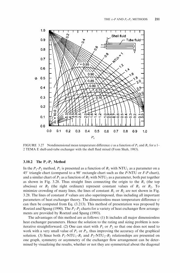
3.10.2 The P1-P2 Method

In the P1-P2 method, P1 is presented as a function of R1 with NTU1 as a parameter on a458 triangle chart (compared to a 908 rectangle chart such as the P-NTU or F-P chart),

and a similar chart of P2 as a function ofR2 with NTU2 as a parameter, both put togetheras shown in Fig. 3.28. Thus straight lines connecting the origin to the R1 (the topabscissa) or R2 (the right ordinate) represent constant values of R1 or R2. Tominimize crowding of many lines, the lines of constant R1 or R2 are not shown in Fig.

3.28. The lines of constant F values are also superimposed, thus including all importantparameters of heat exchanger theory. The dimensionless mean temperature difference can then be computed from Eq. (3.213). This method of presentation was proposed by

Roetzel and Spang (1990). The P1-P2 charts for a variety of heat exchanger flow arrange-ments are provided by Roetzel and Spang (1993).

The advantages of this method are as follows: (1) It includes all major dimensionless

heat exchanger parameters. Hence the solution to the rating and sizing problem is non-iterative straightforward. (2) One can start with P1 or P2 so that one does not need towork with a very small value of P1 or P2, thus improving the accuracy of the graphical

solution. (3) Since both P1-NTU1-R1 and P2-NTU2-R2 relationships are presented onone graph, symmetry or asymmetry of the exchanger flow arrangement can be deter-mined by visualizing the results, whether or not they are symmetrical about the diagonal

FIGURE 3.27 Nondimensional mean temperature difference as a function of P1 andR1 for a 1–

2 TEMA E shell-and-tube exchanger with the shell fluid mixed (From Shah, 1983).

THE -P AND P1-P2 METHODS 211

P1 ¼ P2 axis (the 458 line from the origin). (4) Since the NTU ¼ 1 line is shown, one caneasily recognize the region beyond NTU ¼ 1 where a set of mutually consistent heat

exchanger parameters does not exist (no design is possible). From the visual inspectionpoint of view, in the P1-P2 method, (1) one cannot easily recognize direct asymptoticbehavior of Pwith NTU as in a P-NTU chart, and (2) one cannot recognize P decreasing

with increasing NTU after some maximum value as in the temperature cross case.

3.11 SOLUTION METHODS FOR DETERMINING EXCHANGER

EFFECTIVENESS

In Section 3.4.1.1, differential energy balance and rate equations were derived for acounterflow exchanger. Subsequently, a procedure for determining heat exchanger effec-

tiveness was illustrated based on the analytical model derived. Although no attempt wasmade there to derive formulas for temperature distribution in both fluids and the wall,they can be obtained, as presented in Sections 11.2.1 and 11.2.4. All we derived in Section

3.4.1.1 was the outlet temperature difference ratio and subsequently the "-NTU formula


FIGURE 3.28 P1–P2 chart for a 1–2 TEMA E shell-and-tube exchanger with shell fluid mixed

(From Roetzel and Spang, 1993).

for a counterflow exchanger by integrating compound differential equations acrossthe exchanger surface area (length). In addition to the "-NTU formulas, expressionsfor P-NTU and F factors were presented.

A variety of methods have been used to derive "-NTU or P-NTU formulas for

different heat exchanger flow arrangements. The major methods employed are: analyticalfor obtaining exact solutions, approximate (analytical, seminumerical, and analog),numerical, matrix formalism, and one based on exchanger configuration properties.

These methods have been summarized by Sekulic et al. (1999). The ultimate goal ofeach of these methods is to determine heat exchanger effectiveness. These methodsare described briefly next. More details about the temperature distributions and some

guidelines for determining thermodynamic properties of heat exchangers are given inChapter 11.

3.11.1 Exact Analytical Methods

Three major categories of methods are employed:

1. A direct integration of ordinary and/or partial differential equations from applica-tion of the energy balances and rate equations. Single-pass parallelflow and coun-terflow exchangers and 1–2n TEMA E shell-and-tube exchangers have beenanalyzed by this method.

2. Operational calculus methods. These include the Laplace transform technique andMikusinski operational calculus. Single-pass and multipass crossflow exchangers

and various shell-and-tube heat exchanger flow arrangements have been analyzedby these methods.

3. Transformations of differential equations into integral equations and subsequent

solution of integral equations; Volterra integral equations have been solved foranalyzing an unmixed–unmixed single-pass crossflow exchanger.

3.11.2 Approximate Methods

Semianalytical/numerical methods used for analyzing single-pass and multipass cross-

flow exchangers are a collocation method, Galerkin method, and two-dimensionalRoesser discrete linear image processing method. In the collocation method applied toa two-pass crossflow exchanger, first the Laplace transforms are applied to independentvariables. The resulting equations are coupled at the boundary conditions between passes

and lead to integral equations that can be solved exactly or approximately by the collo-cation andGalerkin methods. When the partial differential equations of a heat exchangermodel are discretized and organized in matrix form, they are similar in form to a discrete

image-processing model. The important advantage of these models is their straightfor-ward computer implementation for the solution.

3.11.3 Numerical Methods

Finite difference, finite volume, and finite element methods have been used for obtaining"-NTU or P-NTU relationships for single and multipass crossflow exchangers and some

shell-and-tube heat exchangers.

SOLUTION METHODS FOR DETERMINING EXCHANGER EFFECTIVENESS 213

3.11.4 Matrix Formalism

The matrix formalism method uses matrix algebra to obtain the P-NTU formulas for anexchanger array (e.g., see Fig. 3.19 to 3.22) or for a complex exchanger which can bebroken into simpler subexchangers whose P-NTU formulas are known. In this method,

using the overall energy balance for each fluid, any two fluid temperatures (e.g., outlettemperatures) can be presented in terms of two remaining independent fluid temperatures(e.g., inlet temperatures) (see, e.g., Table 3.10). The coefficients of independent fluid

temperatures can then be presented in a 2� 2 linear matrix. The overall P value of anexchanger array or a complex exchanger is eventually obtained by proper multiplicationof appropriate 2� 2 matrices. Thus matrix transformation rules are applied using indi-vidual exchanger effectiveness as building blocks to obtain overall effectiveness. Refer to

Sekulic et al. (1999) for further details.

3.11.5 Chain Rule Methodology

For a very complex flow arrangement, the matrix formalism method mentioned above

becomes too difficult to handle, due to the large number of matrices involved and theassociated matrix multiplication and transformation. Our primary interest is in obtainingonly P1 or P2, rather than performing matrix multiplication (which involves all fourterms of each 2� 2 matrix) for a complex heat exchanger configuration or an array.

Hence, only one term of the 2� 2 matrix (P1 or P2) for the overall exchanger is evaluatedthrough matrix multiplication of the corresponding terms of N 2� 2 matrices. In fact,the chain rule methodology offers a scheme to relate an assembly matrix element Mi j

(such as P1) to individual component elements Zi j , Yi j , and so on, without the use ofdirect matrix algebra or matrix multiplication. This is a powerful technique to obtain aclosed-form expression for the effectiveness of many highly complex exchanger config-

urations and assemblies. It can analyze exchangers with multiple (more than two) inlet or


TABLE 3.10 Formulas for Exchanger 2 Terminal Temperatures as Functions of Two Remaining

Terminal Temperatures, P1 and P2

T1;o ¼ ð1� P1ÞT1;i þ P1T2;i T1;i ¼1

1� P1

ðT1;o � P1T2;iÞ

T2;o ¼ P1R1T1;i þ ð1� P1R1ÞT2;i T2;o ¼1

1� P1

fP1R1T1;o þ ½1� P1ð1þ R1Þ�T2;ig

T1;i ¼1

1� P1ð1þ R1Þ½ð1� P1R1ÞT1;o � P1T2;o� T1;i ¼

1

P1R1

½�ð1� P1R1ÞT2;i þ T2;o�

T2;i ¼1

1� P1ð1þ R1Þ½�P1R1T1;o þ ð1� P1ÞT2;o� T1;o ¼

1

P1R1

½P1T2;i þ ð1� P1ÞT2;o�

T1;o ¼1

1� P1R1

f½1� P1ð1þ R1Þ�T1;i þ P1T2;og T2;i ¼1

P1

½�ð1� P1ÞT1;i þ T1;o�

T2;i ¼1

1� P1R1

ð�P1R1T1;i þ T2;oÞ T2;o ¼1

P1

f�½1� P1ð1þ R1Þ�T1;i þ ð1� P1R1ÞT1;og

outlet streams (such as 1–2 TEMA J or H exchangers), unmixed streams between exchan-gers or passes, and the exchanger assembly, which may or may not be coupled only inseries and parallel coupling (i.e., connected by some compound coupling). This chain rulemethodology with examples is presented by Pignotti and Shah (1992). A number of

formulas in Table 3.6 have been determined in the recent past using this methodology.

3.11.6 Flow-Reversal Symmetry

Flow-reversal symmetry refers to identical overall thermal performance (q, ", P1, or F) of

an exchanger under the inversion of flow directions of both fluids in any one exchanger.Such an exchanger can have one or more inlet and outlet streams for fluid 1 and one ormore inlet and outlet streams for fluid 2. This means that q, ", P1, or F of a given

exchanger and an exchanger with the flow direction of both fluids reversed remainsunchanged under the idealizations listed in Section 3.2.1. Thus, the principle of flow-reversal symmetry is valid for all two-fluid individual exchangers. Although in somecases, this statement of flow-reversal symmetry is obvious; in other instances it is a useful

tool to determine whether or not seemingly different exchanger configurations are trulydifferent or the same. For example, consider the two plate exchangers of Fig. 3.29a and b.At first glance, they appear to be quite different. Reversing the flow directions of both

streams of Fig. 3. 29b results in Fig. 3.29c; it will not change the "-NTU (or P1-NTU1)relationship, as mentioned above. The mirror image of Fig. 3.29c is then shown inFig. 3.29d, which will again maintain the "-NTU (or P1-NTU1) relationship invariant.

Thus the flow arrangements of Fig. 3.29a and d are identical within the exchanger; theonly difference is that the directions of fluid 1 in the inlet and outlet manifolds arechanged. Since this is outside the active heat transfer region, it does not have any

effect on " or P1 under the idealizations of Section 3.2.1. Thus, using the principle offlow reversibility, it is shown that the "-NTU (or P1-NTU1) relationships of theseemingly different plate exchangers of Fig. 3.29a and b are identical.

SOLUTION METHODS FOR DETERMINING EXCHANGER EFFECTIVENESS 215

FIGURE 3.29 (a) 1 pass–2 pass plate exchanger; (b) alternative 1 pass– 2 pass plate exchanger;

(c) exchanger of (b) with both fluids reversed; (d) mirror image of the exchanger of (c) (From Shah

and Pignotti, 1989).

Most of the configurations of Table 3.6 are geometrically symmetric (i.e., afterreversal of both fluids, they coincide with the original geometry, except for some trivialtransformation, such as rotation, mirror image, etc.). For such cases, flow reversal sym-metry does not provide any additional information. The geometrically asymmetric cases

are III.1, III.2, III.4, III.10, III.11, III.12, V.3, V.6, V.11, V.12, and V.13 in Table 3.6. Forthese cases, two seemingly different geometries (one shown in the schematics of Table 3.6and the other with both flows reversed) have the same effectiveness; and hence the

effectiveness of the seemingly different configuration is known instantly through theconcept of flow reversibility.

3.11.7 Rules for the Determination of Exchanger Effectiveness with One Fluid Mixed

As presented in Section 3.11.6, the principle of flow reversibility indicates that when thedirections of both fluids are reversed in any two-fluid individual exchangers (not anarray), the exchanger effectiveness " (and P1 and F) does not change. In contrast, con-

sider a multipass or complex configuration exchanger having at least one fluid sideperfectly mixed throughout, the other fluid side being mixed, unmixed, or partiallymixed. If the effectiveness of such an exchanger is known for overall parallelflow (or

counterflow), the effectiveness of the same exchanger configuration with the direction ofonly one fluid (which one is immaterial) reversed [i.e., the resulting overall counterflow(parallelflow)], can be found readily as follows. The effectiveness P1 of the original

exchanger and the effectiveness PP1 of the exchanger with one fluid reversed are relatedas follows (Sekulic et al., 1999):

PP1ðR1;NTU1Þ ¼P1ð�R1;NTU1Þ

1þ R1P1ð�R2;NTU1Þð3:216Þ

Here the subscript 1 refers to the fluid side having no restrictions (i.e., it can be mixed,unmixed, or split). The temperature effectiveness of the mixed fluid (the subscript 2) isthen given by

PP2ðR2;NTU2Þ ¼�P2ð�R2;�NTU2Þ1� P1ð�R2;�NTU2Þ

ð3:217Þ

It must be emphasized that Eq. (3.216) or (3.217) is a mathematical relationship

between values of P of the original and inverted exchangers. PP of the inverted exchangerfor the physical (positive) values of R is related to P of the original exchanger for theunphysical (negative) values of R as shown in Eq. (3.216) or (3.217).

If one of the fluid flow directions is reversed for the exchangers of Eqs. (III.3), (III.7),

and (III.9), Eq. (3.216) can be applied to get the effectiveness of the overall parallelflowexchanger, and hence those configurations are not included in Table 3.6.

3.12 HEAT EXCHANGER DESIGN PROBLEMS

While comparing the "-NTU and MTD methods in Section 3.9, the solution proceduresfor two heat exchanger design problems (rating and sizing) were provided. However,considering seven variables of the heat exchanger design problem [Eq. (3.7)], there are a

total of 21 problems, as shown in Table 3.11. In this table, the dimensionless parameters


TABLE

3.11

DesignProblemsin

TermsofDim

ensionalandDim

ensionless

Parameters

Dim

ensionalParameters

Dim

ensionless

Groups

Problem

UA

_ mm1orC

1_ mm2orC

2T1;i

T1;o

T2;i

T2;o

P1

P2

NTU

1NTU

2R

1R

2

Sizing

1�

�

��

2�

�

��

3�

�

��

4�

�

��

5�

�

��

6�

�

��

Rating

7

��

��

8

��

��

9

�

�

��

10

�

��

�

11

��

�

�

12

�

��

�

13

�

��

�

14

�

�

�

��

�

�15

�

�

�

�

�

�16

�

�

�

�

��

�17

�

�

�

��

�18

��

�

�

��

�19

�

�

�

��

�20

�

�

�

��

�

�21

�

�

��

�

�Source:

Data

from

Baclic

(1990).

a�,

Unknown;,

knownparameter.

217

are also included with known or unknown values based on the dimensional variables. Ifonly one of the temperatures is known, we evaluate the specific heat at that temperaturefor the determination/estimate of C and hence R; eventually, once we know both tem-peratures, an iteration may be needed. If specific heats are treated as constant, C1 and C2

in the equations above are interchangeable with _mm1 and _mm2. Also, we have presentlyconsidered theUA product as one of the design parameters. We discuss separatingU andA when we discuss the detailed sizing problem in Chapter 9. In the foregoing count, we

have not added q since q can readily be calculated from the overall energy balance [Eq.(3.5)] or the rate equation [Eq. (3.6) or (3.12)]. Alternatively, if q is given, one of thetemperatures or the flow rates (heat capacity rate) could be unknown in Table 3.11. We

could classify the first six problems as variations of the sizing problem and the next 15problems as a variation of the rating problem. Using the P-NTU method, these 21problems can be solved as follows.

1. For problems 1 to 6, P1 (also P2) and R1 are known through the heat balance.Hence, NTU1 can be calculated from the P-NTU formula for a given flow arrange-

ment, either straightforward or iteratively, depending on whether NTU can beexpressed explicitly (see Table 3.4) or implicitly (see Table 3.6).

2. For problem 7, since all four temperatures are known, both P1 and R1 are known

through their definitions [Eqs. (3.96) and (3.105)]. Hence, NTU1 can be calculatedas mentioned in the preceding paragraph for a given flow arrangement. ThenC1 ¼ UA=NTU1 and C2 ¼ C1=R1. Knowing the specific heats of the given fluids,

one can determine _mm1 and _mm2.

3. For problems 8 to 13, NTU1 and R1 are known. Hence, determine P1 using theappropriate formula from Table 3.6. Now knowing P1, R1, and the definition of

P1, compute the unknown temperatures using the formulas given in Table 3.10.

4. Problems 14 and 16 can only be solved iteratively, with the solution procedurefor problem 14 as follows. Assume _mm1 (or C1). Calculate R2 ð¼ C2=C1Þ. From the

problem specifications, NTU2 ¼ UA=C2 and q ¼ C2jT2;i � T2;oj are known.Hence, knowing NTU2 and R2 for a given flow arrangement, determine P2

using the appropriate formula from Table 3.6. Subsequently, compute T1;i from

the definition of P2, and C1 from the energy balance C1jðT1;i � T1;oÞj ¼ q. Withthis new value of C1, repeat all the calculations above. Continue to iterate until thesuccessive values of C1 converge within the accuracy desired. The solution pro-

cedure for problem 16 is identical to that for problem 14 just described, startingwith assuming _mm2 (or C2) and computing R1 and NTU1. The solution procedurefor problem 15 is relatively straightforward. In this case, P2 and NTU2 are given.From the known P-NTU formula from Table 3.6, compute R2 iteratively (such

as using the Newton–Raphson method) since it is an implicit function of P2 andNTU2. Similarly, P1 and NTU1 are known for problem 17 and determineiteratively R1 from the known P-NTU formula of Table 3.6.

5. Problems 18 and 20 can only be solved iteratively, with the solution procedure forproblem 18 as follows. Assume C2 and hence determine R1 ð¼ C1=C2Þ. Also,compute NTU1 ð¼ UA=C1Þ from the input. For a given flow arrangement, deter-

mine P1 using the appropriate formula from Table 3.6. Subsequently, compute T1;i

from the definition of P1. Finally, calculate C2 from the overall energy balanceC1ðT1;i � T1;oÞ ¼ C2ðT2;o � T2;iÞ. With this new value of C2, repeat all the calcula-

tions above. Continue to iterate until successive values of C2 converge within the


desired accuracy. The solution procedures for problem 20 is identical to that forproblem 18 just described, starting with assuming C1 and computing R2 andNTU2.

The solution procedure for problem 19 is relatively straightforward. In this case,

P2 and NTU1 are known. For the given flow arrangement, select the P1-NTU1

formula from Table 3.6 and replace P1 by P2=R1 [see Eq. (3.98)]. The resultingequation has only one unknown, R1, since NTU1 and P2 are known; and R1 is

implicit. It can be computed iteratively using, for example, the Newton–Raphsonmethod. Similarly, P1 and NTU2 are known in problem 21, and compute R2

iteratively after replacing P1 by P2R2 in the appropriate P-NTU formula of

Table 3.6. See the footnote of Table 3.6 for how to convert P1-NTU1-R1 formulasinto P2-NTU2-R2 formulas.

SUMMARY

This chapter is very important to the book. We have presented in considerable detail thebasic thermal design theory for recuperators or exchangers with no moving parts orperiodic flows as in regenerators. Through the problem formulations, it is shown that

there are six independent and one or more dependent variables for the exchanger thermaldesign problem for any flow arrangement. The solution to this problem can be presentedin terms of "-NTU, P-NTU, MTD, -P and P1-P2 methods. The exchanger rating orsizing problem can be solved by any of these methods and will yield the identical solution

within the numerical error of computation. Theoretical details are presented for the "-NTU, P-NTU, and MTD methods in the text for an understanding of concepts, thesemethods, and their advantages and disadvantages. Many idealizations are made to

simplify the complex heat exchanger design problem to obtain the solution in terms of"-NTU, P-NTU, and MTD parameters. A thorough understanding of the concepts andresults presented in this chapter will provide a strong foundation for rating, sizing, and

analysis of industrial heat exchangers.

REFERENCES

Baclic, B. S., 1990, "-Ntu analysis of complicated flow arrangements, in Compact Heat Exchangers:

A Festschrift for A. L. London, R. K. Shah, A. D. Kraus, and D. Metzger, eds., Hemisphere

Publishing, Washington, DC, pp. 31–90.

Bell, K. J., 1998, Approximate sizing of shell-and-tube heat exchangers, in Heat Exchanger Design

Handbook, G. F. Hewitt, exec. ed., Begell House, New York, Vol. 3, Sec. 3.1.4.

Kandlikar, S. G., and R. K. Shah, 1989, Asymptotic effectiveness–NTU formulas for multipass

plate heat exchangers, ASME J. Heat Transfer, Vol. 111, pp. 314–321.

McAdams, W. H., 1954, Heat Transmission, 3rd ed., McGraw-Hill, New York, pp. 129–131.

Mueller, A. C., 1967,New Charts for TrueMean Temperature Difference in Heat Exchangers,AIChE

Paper 10, 9th National Heat Transfer Conf., Seattle, WA.

Pignotti, A., and G. O. Cordero, 1983, Mean temperature difference in multipass crossflow, ASME

J. Heat Transfer, Vol. 105, pp. 584–591.

Pignotti, A., and R. K. Shah, 1992, Effectiveness-number of transfer units relationships for heat

exchanger complex flow arrangements, Int. J. Heat Mass Transfer, Vol. 35, pp. 1275–1291.

SUMMARY 219

Roetzel, W., and B. Spang, 1990, Verbessertes Diagramm zur Berechnung von Warmeubertragern,

Warme-und Stoffubertragung, Vol. 25, pp. 259–264.

Roetzel, W., and B. Spang, 1993, Design of Heat Exchangers, in VDI Heat Atlas, VDI-Verlag

GmbH, Dusseldorf, Germany, Sect. Ca, p. 18.

Sekulic, D. P., R. K. Shah, and A. Pignotti, 1999, A review of solution methods for determining

effectiveness–NTU relationships for heat exchangers with complex flow arrangements, Appl.

Mech. Rev., Vol. 52, No. 3, pp. 97–117.

Shah, R. K., 1983, Heat exchanger basic design methods, in Low Reynolds Number Flow Heat

Exchangers, S. Kakac, R. K. Shah, and A. E. Bergles, eds., Hemisphere Publishing, Washington,

DC, pp. 21–72.

Shah, R. K., and A. Pignotti, 1989, Basic Thermal Design of Heat Exchangers, Report Int-8513531,

National Science Foundation, Washington, DC.

REVIEW QUESTIONS

Where multiple choices are given, circle one or more correct answers. Explain youranswers briefly.

3.1 Thermal and electrical analogy exists for:

(a) resistances in parallel (b) resistances in series

(c) power (d) time constant

3.2 The true mean temperature difference for nonuniform U is defined as:

(a) �Tm ¼ 1

A

ð

A�T dA (b) �Tm ¼ 1

q

ð

q�T dq

(c)1

�Tm

¼ 1

q

ð

q

dq

�T

3.3 Fouling generally provides:

(a) an increase in heat transfer coefficient

(b) an increase in thermal resistance to heat flow path

(c) higher outlet temperatures (d) none of these

3.4 Explicit basic principles used in deriving "-NTU relationships or F factors are:

(a) second law of thermodynamics (b) energy balances

(c) rate equation (d) equation of state

3.5 The explicit rate equation used in the heat exchanger analysis is:

(a) dq ¼ jChdThj (b) "hCh ¼ "cCc

(c) dq ¼ U�T dA (d) q ¼ ChðTh;i � Th;oÞ(e) q ¼ "CminðTh;i � Tc;iÞ

3.6 The energy balance equation used in the heat exchanger analysis, from thoseequations in Question 3.5, is (check as appropriate)

(a) _______ (b) _______ (c) _______ (d) _______ (e) _______


3.7 Consider a heat exchanger for which C* is near unity. The hot- and cold-fluidtemperatures are shown in Fig. RQ3.7 as functions of the position in theexchanger. In this figure,

(a) sketch the variation of wall temperature with position (neglecting wall resis-tance) when ðhAÞh ðhAÞc.

(b) repeat part (a) when ðhAÞc ðhAÞh.

3.8 The "-NTU and MTD methods employ the following assumptions:

(a) variable heat transfer coefficients (b) two-dimensional analysis

(c) longitudinal heat conduction negligible

(d) variable velocity and temperature profiles at the entrance

3.9 The perfect (ideal) heat exchanger, providing the maximum possible heat transferrate, has the following things in common with the actual heat exchanger withconstant cp:

(a) flow arrangement (b) outlet temperatures (c) inlet temperatures

(d) surface area (e) flow rates (f) none of these

(g) all of these

3.10 A high number of transfer units NTUs (let’s say, 100) is generally obtainable inaðnÞ:(a) physically very large exchanger (b) exchanger with high flow rates

(c) high effectiveness exchanger (d) small exchanger

(e) can’t tell

3.11 The total NTUs of a two-pass cross-counterflow exchanger is 4. The hot airenters at 3158C and leaves at 1508C on one side. On the other side, 450 kg/hcold air enters at 258C and leaves at 2608C. The approximate hot-air flow rate

should be:

(a) 450 kg/h (b) 325 kg/h (c) 640 kg/h (d) can’t tell

3.12 The effectiveness of the exchanger of Question 3.11 is:

(a) 71% (b) > 85% (c) 59% (d) 81%

REVIEW QUESTIONS 221

FIGURE RQ3.7

3.13 A heat exchanger has been designed so that Cc ¼ 20 kW=K and Ch ¼ 40 kW=K.The number of transfer units on the cold side, ntuc ¼ 6, and that on the hot side,ntuh ¼ 4:5. Recall ntuside ¼ ð�ohA=CÞside. The total NTUs for the exchanger,neglecting wall resistance and fouling, is:

(a) 10.5 (b) 1.5 (c) 3.6 (d) 1.33

3.14 What is the ratio of hot- and cold-side convective thermal resistances in Question

3.13?

(a) 1.33 (b) 2.67 (c) 2 (d) 0.667

3.15 The terminal temperatures of a particular heat exchanger are: hot fluid: 1208C,508C; cold fluid: 408C, 808C. The effectiveness of this exchanger is approximately:

(a) 87% (b) 50% (c) 75% (d) 38%

3.16 The heat capacity rate ratio C* for the heat exchanger of Question 3.15 is:

(a) 1.75 (b) 0.38 (c) 0.64 (d) 0.57

3.17 The heat exchanger of Question 3.15 may have a parallelflow arrangement.

(a) true (b) false (c) can’t tell

3.18 If you consider the heat exchanger of Question 3.15 as counterflow, the tempera-ture distribution in the exchanger will be:

(a) concave up (b) convex up (c) linear

3.19 If you consider the heat exchanger of Question 3.15 as a crossflow unit with bothfluids unmixed, the log-mean temperature difference �Tlm is approximately:

(a) 708C (b) 558C (c) 518C (d) 408C (e) 228C

3.20 In a hypothetical counterflow gas turbine regenerator, having the same heat capa-

city rate for both fluids, the design NTU and effectiveness are 0.5 and 33%,respectively. If at part-load operation, NTU doubles, the corresponding effective-ness is:

(a) 66% (b) 50% (c) 83% (d) 40%

3.21 Other things being equal (including identical heat transfer surfaces), a multipass

cross-counterflow heat exchanger designed for a particular set of specifications(i.e., given ", C*, flow rates, and flow lengths) will have a shorter noflow (stack)height dimension than a single-pass crossflow heat exchanger.

(a) It depends on the surface geometries. (b) true (c) false

(d) It depends on the capacity rate ratio.

3.22 The effectiveness of a single-pass crossflow heat exchanger with both fluidsunmixed, and with equal heat capacity rates, approaches the following limit asthe NTU is increased to infinity:

(a) 50% (b) 62% (c) 67% (d) 100%

3.23 In a steam condenser, the steam is effectively at a constant temperature of 508Cthroughout the heat exchanger, while the temperature of cooling water increasesfrom 208C to 318C as it passes through the condenser. The NTU for this heatexchanger is

(a) 1.00 (b) 0.367 (c) 4.55 (d) 0.457 (e) 2.19


3.24 Suppose that we desire to increase the water outlet temperature to 408C in the heatexchanger of Question 3.23 at the same flow rate. The surface area of thisexchanger required (considering that U ¼ constant) should be increased by afactor of:

(a) 2.40 (b) 1.29 (c) 1.0 (d) 0.67

3.25 Suppose in Question 3.23 that the flow rate of the cooling water is doubled.

Describe qualitatively how the thermal behavior of the exchanger will change.Idealize no subcooling of steam. Consider all the implications you can think of.

3.26 The curves in Fig. RQ3.26a and b represent the temperature profiles in twodifferent counterflow exchangers having the same cold fluids and the same coldfluid flow rate in each exchanger. The heat transfer rate of exchanger A is asfollows compared to that of exchanger B:

(a) higher (b) lower (c) same (d) can’t tell

3.27 Circle the following statements as true or false.

(a) T F The F factor represents exchanger effectiveness.

(b) T F The F factor is a ratio of the true mean temperature difference in acounterflow exchanger to that in the actual exchanger.

(c) T F The F factor is a ratio of the counterflow NTU to NTU of the actual

exchanger under consideration.

(d) T F The higher F factor means generally higher NTU.

(e) T F In the asymptotic region of the F-factor curves in Fig. 3.26, a slightchange in the exchanger thermal effectiveness means a large changein the F factor, and hence a large change in q and instability in the

exchanger performance q ¼ UAF �Tlmð Þ.(f) T F The F factor increases with an increasing number of shell passes at

the same total NTU for overall counterflow.

(g) T F A decreasing LMTD for an exchanger means increasing its heatexchanger effectiveness.


FIGURE RQ3.26

3.28 A value close to unity of the log-mean temperature correction factor F means:

(a) exchanger effectiveness approaching 100%

(b) performance approaching that of a crossflow exchanger with both fluids

unmixed

(c) performance approaching that of a counterflow exchanger

(d) can’t tell

3.29 (a) When is it true that �Tlm for counterflow ¼ �Tlm for parallelflow for a givenduty?

(b) When is it true that �Tlm ¼ ð�T1 þ�T2Þ=2 for a single-phase counterflow

exchanger? (Mention the R value.)

(c) When is �Tlm ¼ ð�T1 þ�T2Þ=2 true for a single-phase parallelflow

exchanger?

(d) When is it true that �Ta ð¼ Ta;o � Ta;iÞ ¼ �Tlm for a steam condenser wherethe subscript a denotes the air side?

3.30 TEMA E shell-and-tube exchangers are generally designed with an approximateminimum log-mean temperature difference correction factor F of:

(a) 0.90 (b) 0.80 (c) 0.40 (d) 0.98 (e) no limit

Hint: No temperature cross is desired in the exchanger.

3.31 Hot (150 to 1008C) and cold (50 to 758C) fluids undergo the same temperaturechanges (as indicated in parentheses) in a counterflow exchanger and a parallel-flow exchanger. For the identical temperature changes and flow rates (same U),

the heat transfer surface area required for the counterflow exchanger compared tothat for the parallelflow exchanger is:

(a) 1.00 (b) 1.14 (c) 0.877 (d) 2.00

3.32 Which of the following dimensionless groups can have values ranging from 0 to 1only?

(a) " (b) NTU1 (c) F (d)

(e) R1 (f) NTU (g) P1 (h) C*

3.33 Which of the following statements are always true?

(a) P1 � " (b) R1 � C* (c) NTU1 � NTU

3.34 In a heat exchanger, the effectiveness generally increases with:

(a) increasing NTU (b) increasing C*

(c) increasing the mixing of fluids at a cross section

(d) increasing F

3.35 For the same surface areas, fluid flow rates, and inlet temperatures, arrange thefollowing flow arrangements from lowest to highest effectiveness:

(a) unmixed–unmixed (b) mixed–mixed (c) mixed–unmixed

(d) one fluid partially unmixed, other unmixed

3.36 Circle the statements that are true about multipass exchangers.

(a) Multipass exchangers are always of crossflow type.


(b) A multipass counterflow exchanger can be more efficient than a single-passcounterflow exchanger having the same NTU and C*.

(c) A multipass overall parallelflow exchanger can be more efficient than a single-

pass parallelflow exchanger having the same NTU and C*.

3.37 The temperature approach for a counterflow exchanger of infinite surface area is:

(a) indeterminate (b) zero

(c) a very large value (d) can’t tell

3.38 In a single-pass counterflow heat exchanger with a fixed heat duty, the closer the

temperature approach, the more heat transfer surface area is required.

(a) true (b) false (c) can’t tell in general

3.39 The true mean temperature difference in an exchanger can be determined by:

(a) �Tm ¼ F �Th (b) �Tm ¼ �Tlm

(c) �Tm ¼ "�Tmax

NTU(d) �Tm ¼ �Th

NTUð Þc3.40 An nð>1Þ 1–2 TEMA G exchanger in series in overall counterflow may be

analyzed using Eq. (3.131).

(a) true (b) false (c) can’t tell

3.41 The dimensionless temperature difference can be presented as the followingfunctional relationship for a given heat exchanger flow arrangement. Subscripts1 and 2 refer to fluid 1 and 2 sides, respectively.

(a) ¼ �ðP1;P2Þ (b) ¼ �ðNTU1;NTU2Þ (c) ¼ �ðR1;R2Þ(d) ¼ �ðP1;NTU2Þ (e) can’t tell

3.42 The exchanger effectiveness " can be presented as the following functional rela-tionship for a given heat exchanger flow arrangement. Subscripts 1 and 2 refer tofluid 1 and 2 sides, respectively.

(a) " ¼ �ðP1;P2Þ (b) " ¼ �ðNTU1;NTU2Þ(c) " ¼ �ðR1;R2Þ (d) " ¼ �ðP1;NTU2Þ(e) can’t tell

3.43 For a given exchanger and specified operating conditions, one can calculateF1 ¼ �ðP1;R1Þ or F2 ¼ �ðP2;R2Þ. Is it correct that F1 ¼ F2 in general?

(a) yes (b) no (c) can’t tell

3.44 In a heat exchanger, engine oil with a 0.2 kg/s flow rate and 1308C inlet tempera-

ture is being cooled by water having a 0.438 kg/s flow rate at 908C inlet. The engineoil and water specific heats are 2.3 and 4.2 kJ/kg �K, respectively. What is themaximum possible exchanger effectiveness if it is a counterflow exchanger?

(a) 100% (b) 25% (c) 50% (d) 80% (e) can’t tell

3.45 What is the maximum possible exchanger effectiveness if the exchanger ofQuestion 3.44 is a parallelflow exchanger?

(a) 100% (b) 25% (c) 50% (d) 80% (e) can’t tell

3.46 In a counterflow double-pipe heat exchanger, cold water enters the annulus at

208C and leaves at 658C. In the inner pipe, hot water enters at 1108C and leaves


at 658C. The length of the exchanger is 2m. We would like to increase the outlettemperature of the cold water to 808C by increasing the length of the double-pipeexchanger without changing the inlet temperatures and flow rates of both fluidsand also keeping constant the tube diameters of the exchanger. Make appropriate

idealizations and find the new length of the exchanger as:

(a) 2 m (b) 3 m (c) 4 m (d) 5 m (e) can’t tell

3.47 A 2-ton window air-conditioner needs to remove 8.4 kW of heat from its con-denser. In the condenser, the inlet temperature of air is 388C and the refrigerant

condenses at 578C. Ignore the effect of desuperheating and subcooling in thecondenser. UA for this air-conditioner is 700W/K. Assume the specific heat ofair as 1.0 kJ/kg �K. Use any appropriate information from this or any other book,

and determine the airflow rate through the condenser as:

(a) 1 kg/s (b) 0.7 kg/s (c) 0.5 kg/s (d) 1.5 kg/s (e) can’t tell

Hint: Assume the exponent to e to be an integer.

3.48 For Question 3.47, the air temperature rise will be:

(a) 108C (b) 68C (c) 128C (d) 208C (e) can’t tell

3.49 A 1–2 TEMAE shell-and-tube exchanger has the temperature effectiveness of 0.09and heat capacity rate ratio of 10. At this operating point, the log-mean tempera-

ture difference correction factor F will be approximately:

(a) 0.65 (b) 0.75 (c) 0.85 (d) 0.95 (e) can’t tell

3.50 A heat exchanger is made of connecting two crossflow subexchangers designedhaving total NTU1 ¼ 2 and overall R1 ¼ 0:5. Arrange the following design alter-

natives from higher to lower effectiveness P1.

(a) series coupling with overall parallelflow

(b) series coupling with overall counterflow

(c) parallel coupling with fluid 1 in series

(d) can’t tell

3.51 An unmixed–unmixed crossflow exchanger has " ¼ 60% and F ¼ 0:98 at

NTU ¼ 1 for C* ¼ 0:2. To demonstrate how F varies with NTU, we increaseNTU ¼ 3 at C* ¼ 0:2. In that case, the exchanger effectiveness " increases to90%. The corresponding F value will be:

(a) 0.98 (b) 0.88 (c) 1.00 (d) 0.01

3.52 Consider a clean counterflow heat exchanger with desired " ¼ 85% at C* ¼ 1. Ifthe heat leakage to the ambient is 2%, approximately how much will be anincrease in heat transfer surface area on each fluid side to increase the cold-fluid

temperature at the same level of the no-heat-leakage case? Consider all othergeometric and operating parameters of the exchanger remaining the same andð�ohAÞ* ¼ 1.

(a) 0% (b) 2% (c) 6.4% (d) 12.8% (e) can’t tell


PROBLEMS

3.1 The typical temperature distributions for hot and cold fluids in a counterflowexchanger are shown in the left-hand sketch of Fig. 1.50 for Ch > Cc. Using the

energy balance and rate equations, show why the temperature distributions mustbe convex up. Hint: First show that ðTh � TcÞ increases as x increases.

3.2 Discuss in detail where each of the assumptions listed in Section 3.2.1 is invoked in

the set of Eqs. (3.2), (3.4), (3.5), and (3.6). Alternatively, show how one or more ofthese equations could be changed if those assumptions were not invoked.

3.3 The required NTU for a given exchanger is 2.0. If Cc ¼ 10;000W=K,Ch ¼ 40;000W=K, and the thermal resistance Rw of the wall separating hot and

cold fluids is 10�5 K/W, find ntuh and ntuc when the convective resistances of hotand cold sides are estimated to be equal. What would the values be if the thermalresistance of the wall is neglected?

3.4 Explain the physical reasoning why " ¼ 1� e�NTU for all flow arrangements whenC* ¼ 0.

3.5 (a) For a typical counterflow heat exchanger, explain briefly the change in theeffectiveness as the flow rate of the cold fluid is decreased slowly from some

initial value to near zero. Note that we are not interested in transient effects,just a series of steady-state operating conditions. See Fig. 1.50b for the initialtemperature profiles.

(b) Explain briefly the effect on the temperature drop of the hot fluid, �Th.

3.6 In a single-pass crossflow exchanger with both fluids unmixed, it has been deter-mined that the hot and cold streams should leave the exchanger at the same mean

temperature (i.e. Tc;o ¼ Th;oÞ. The following data are given for the exchanger:Th;i ¼ 2508C, Tc;i ¼ 308C, _mmh ¼ 0:15 kg=s, _mmc ¼ 0:60 kg=s, cp;h ¼ 2000 J/kg �K,cp;c ¼ 1000 J=kg �K, and U ¼ 1000W=m2 �K. Determine (a) the required heat

exchanger area (m2); (b) the total heat transfer rate between the hot and coldstreams (W); (c) the outlet temperatures Tc;o and Th;o (8C); (d) the effectivenessof the heat exchanger; and (e) which (if any) of the answers to parts (a) through (d)

would be different if the heat exchanger were, instead, a single-pass counterflow.Explain. Be sure to address each of parts (a) through (d).

3.7 Determine the heat transfer surface area required for a heat exchanger constructedfrom a 25.4mmOD tube to heat helium from �78C to 08C using hot water at

858C. The water and helium flow rates are 0.6 and 2.4 kg/s. Helium flows withinthe tubes. The overall heat transfer coefficient is 120W/m2 �K. The specific heatsfor water and helium are 4.18 and 5.20 kJ/kg �K, respectively. Consider (a) a

counterflow exchanger, and (b) a 1–2 TEMA E exchanger. Solve the problemby both the "-NTU and MTD methods.

3.8 At 80 km/h, the inlet temperature of air to an automobile radiator is 37.88C.Water enters at 98.98C with a flow rate of 1.89 kg/s and leaves with a temperature

of 93.38C. UA for this radiator is 960.6W/K. Determine the airflow rate and airoutlet temperature for this radiator using both the "-NTU and MTD methods.Consider cp for air and water as 1.01 and 4.19 kJ/kg �K, respectively. The radiator

is unmixed on the air side and mixed on the water side.

PROBLEMS 227

3.9 An automobile radiator has a heat transfer rate q ¼ 98:45 kW. Air and water flowrates are 3.86 and 3.00 kg/s, respectively, and air and water inlet temperatures are43 and 1158C. The specific heat for air and water are 1.00 and 4.23 kJ/kg �K,respectively. Consider the radiator as a crossflow heat exchanger with both fluids

unmixed.

(a) Determine the exchanger effectiveness ", the number of transfer units NTU,

and UA.

(b) Determine the true mean temperature difference �Tm for heat transfer.

(c) Determine the F factor. Is the calculated value of F reasonable? If not, why?

(d) Describe by means of a thermal circuit the makeup of (UAÞ�1, and provideyour estimates of the component resistances expressed as a percentage of theoverall resistance ðUAÞ�1.

3.10 Derive Eq. (3.131) for a four-pass arrangement and demonstrate that it reduces to

P1 ¼4Pp

1þ 3Pp

for C * ¼ 1

1� e�NTU for C * ¼ 0

8

><

>:

3.11 Three exchangers identical to the crossflow exchanger of Problem 3.6 are placed in

a multipass overall counterflow arrangement with the same inlet temperatures andflow rates. Find the overall effectiveness of this arrangement and the outlet fluidtemperatures.

3.12 In the text, the exchanger overall effectiveness " (P1) for a multipass overall

counterflow exchanger is given by Eq. (3.131) for the case when the NTU perpass is equal. The objective of this problem is to calculate " for a multipass overallcounterflow exchanger when the NTU per pass is not equal. Consider a counter-flow exchanger with crossflow headers as a three-pass exchanger (Fig. P3.12).

(a) Derive an algebraic expression for an overall effectiveness

" ¼ �ð"1; "2; "3;C *Þ

Then show that for C* ¼ 1 and "1 ¼ "3, it reduces to

" ¼ 3 "1 "2 �2 "1 � "22 "1 "2 � "1 �1


FIGURE P3.12

(b) Harrison Model TR regenerator (for a 12,000-hp GE Frame 3000 marine gasturbine for a Chevron tanker) may be considered as having NTU ¼ 4 andC* ¼ 1. Obtain its effectiveness considering it as a true counterflow heatexchanger. Next approximate it as having two crossflow (unmixed–unmixed)

headers with a counterflow core, as shown in part (a) with NTU1 ¼ NTU3 ¼ 1and NTU2 ¼ 2. Evaluate the overall effectiveness. How good is this approx-imation?

3.13 Consider a single-pass crossflow exchanger with one fluid mixed and NTU ¼ 5

and C* ¼ 1.

(a) Divide this exchanger into two equal passes (so that NTUp ¼ 2:5) and arrangethe two passes into overall counterflow arrangement and obtain the exchanger

overall effectiveness. Repeat this procedure by dividing the original exchangerinto three passes and arranging them in an overall counterflow arrangement,and subsequently obtain the exchanger overall effectiveness. Repeat this

procedure by dividing the original exchanger into four and five passes andsubsequently, obtain the exchanger effectiveness for overall counterflowarrangement. Make a plot of this crossflow exchanger effectiveness as a

function of the number of passes. Compare this curve with the effectivenessof a single-pass counterflow exchanger having NTU ¼ 5 and C* ¼ 1. Discussthe results.

(b) Repeat the complete part (a) using an arrangement of n passes ð2 � n � 5Þ inoverall parallelflow arrangement. Plot the results on the same graph as that ofpart (a) and compare them with the effectiveness of a single-pass parallelflow

exchanger having NTU ¼ 5 and C* ¼ 1. Discuss the results.

3.14 A counterflow heat exchanger is currently used to heat fluid A by fluid C. A needhas arisen to heat a second process stream B, and it has been proposed to do thisby adding another section of exchanger to the existing unit (see Fig. P3.14). For

the data given below and on the figure:

(a) Determine the extra heat exchanger area (i.e., the area of section II) requiredheating fluid B from 25 to 758C.

(b) What is the effectiveness of section II?

(c) Suppose that the heat exchanger area of section I was very much larger than

0.75m2. What would happen to your answer to part (a)? Explain briefly.

Data: The heat exchanger area of section I ¼ 0:75m2. For each of sections I andII,U ¼ 250W=m2 �K. For fluid A: _mm ¼ 0:10 kg=s, cp ¼ 2000 J=kg �K. For fluid B:_mm ¼ 0:30 kg=s, cp ¼ 1000 J=kg �K. For fluid C: _mm ¼ 0:20 kg=s, cp ¼ 1250 J=kg �K.

PROBLEMS 229

FIGURE P3.14

3.15 Given Th;i ¼ 608C, Th;o ¼ 43:38C, Tc;i ¼ 26:78C, and Tc;o ¼ 40:68C, calculate thetrue-mean temperature difference for (a) parallelflow, (b) counterflow, (c) single-pass crossflow with both fluids unmixed, (d) single-pass crossflow with cold fluidunmixed and hot fluid mixed, and (e) a 1–2 TEMA E exchanger. Also determine

the exchanger effectiveness for each case.

3.16 To calculate�Tm for any flow arrangement (except for parallelflow), we calculateit from

�Tm ¼ F �Tlm

where F is the correction factor applied to the logarithmic temperature difference

�Tlm for a hypothetical (or actual) counterflow exchanger operating at the sameRand the same terminal temperatures. This�Tlm is obtained from Eq. (3.172) usingEq. (3.173). Now consider that we use the same counterflow �Tlm definition for aparallelflow exchanger [i.e., Eq. (3.172) in conjunction with Eq. (3.173) and not

Eq. (3.174)]. In this case, F will not be unity, but it will be

F ¼ Rþ 1

R� 1

ln 1� RPð Þ= 1� Pð Þ½ �ln 1� 1þ Rð ÞP½ �

Derive this equation for F for a parallelflow exchanger.

3.17 Lubricating oil at a temperature of 608C enters a 10mm diameter tube with avelocity of 2.0 m/s. The tube surface is maintained at 308C. Calculate the tubelength required to cool the oil to 458C. Consider the following properties for oil:

¼ 865 kg=m3, k ¼ 0:14W=m �K, cp ¼ 1780 J=kg �K, and � ¼ 0:0078 Pa � s.For oil flow in the tube, the heat transfer coefficient h ¼ 51:2W=m2 �K.

3.18 A shell-and tube exchanger is required to cool the hot oil from 2408C to 908C.After some process, the same oil returns to the exchanger at 408C and leaves at1908C. Assume a negligible change in the specific heat of oil in the temperature

range 110 to 1708C.

(a) If you design one 1–2 TEMA E shell-and-tube exchanger, would there be a

temperature cross?

(b) Is it possible to design one 1–2 TEMA E exchanger to meet the requiredspecifications, and why?

(c) What minimum number of 1–2 TEMA E exchangers in series would yourequire to eliminate the temperature cross? Hint: Use an appropriateequation from Eqs. (3.131)–(3.139). Specify any idealization you may

make.

(d) What would be the overall arrangement of two fluids in part (c)? Tell whetheror not you could use an alternate (opposite) flow arrangement and why.

(e) What would be the F factor for part (c)?

3.19 Two identical single-pass counterflow exchangers are used for heating waterðcp ¼ 4:2 kJ=kg �K) at 258C with the hot oil ðcp ¼ 2:1 kJ=kg �K) at 1208C. Thewater and oil flow rates are 1 and 4 kg/s, respectively. The heat exchangers are

connected in series on the water side and in parallel on the oil side, as shown in


Fig. P3.19. The oil flow rate splits equally between the two exchangers at theinlet and rejoins at the exit. Use U ¼ 420W=m2 �K and Apass ¼ 10m2 for each

exchanger. Determine the outlet temperatures of the water and oil.

PROBLEMS 231

FIGURE P3.19

ilovepdf.com split 3

Documents