Image Alignment and Stitching:

A Tutorial1

Richard Szeliski

Preliminary draft, September 27, 2004

Technical Report

MSR-TR-2004-92

This tutorial reviews image alignment and image stitching algorithms. Image align-ment (registration) algorithms can discover the large-scale (parametric) correspon-

dence relationships among images with varying degrees of overlap. They are ideallysuited for applications such as video stabilization, summarization, and the creationof large-scale panoramic photographs. Image stitching algorithms take the alignment

estimates produced by such registration algorithms and blend the images in a seam-less manner, taking care to deal with potential problems such as blurring or ghosting

caused by parallax and scene movement as well as varying image exposures. This tu-torial reviews the basic motion models underlying alignment and stitching algorithms,

describes effective direct (pixel-based) and feature-based alignment algorithms, anddescribes blending algorithms used to produce seamless mosaics. It closes with a dis-

cussion of open research problems in the area.

Microsoft Research

Microsoft CorporationOne Microsoft Way

Redmond, WA 98052

http://www.research.microsoft.com

1A shorter version of this report will appear inMathematical Models of Computer Vision: The Handbook.

Contents

1 Introduction 1

2 Motion models 22.1 2D (planar) motions . . . . . . . . . . . . . . . . . . . . . . . . . . . . . . .. . . 32.2 3D transformations . . . . . . . . . . . . . . . . . . . . . . . . . . . . . . .. . . 5

2.3 Cylindrical and spherical coordinates . . . . . . . . . . . . . .. . . . . . . . . . . 82.4 Lens distortions . . . . . . . . . . . . . . . . . . . . . . . . . . . . . . . . .. . . 10

3 Direct (pixel-based) alignment 113.1 Error metrics . . . . . . . . . . . . . . . . . . . . . . . . . . . . . . . . . . . .. 113.2 Hierarchical motion estimation . . . . . . . . . . . . . . . . . . . .. . . . . . . . 14

3.3 Fourier-based alignment . . . . . . . . . . . . . . . . . . . . . . . . . .. . . . . 153.4 Incremental refinement . . . . . . . . . . . . . . . . . . . . . . . . . . . .. . . . 193.5 Parametric motion . . . . . . . . . . . . . . . . . . . . . . . . . . . . . . . .. . . 23

4 Feature-based registration 264.1 Interest point detectors . . . . . . . . . . . . . . . . . . . . . . . . . .. . . . . . 274.2 Feature matching . . . . . . . . . . . . . . . . . . . . . . . . . . . . . . . . .. . 28

4.3 Geometric registration . . . . . . . . . . . . . . . . . . . . . . . . . . .. . . . . 314.4 Direct vs. feature-based . . . . . . . . . . . . . . . . . . . . . . . . . .. . . . . . 33

5 Global registration 335.1 Bundle adjustment . . . . . . . . . . . . . . . . . . . . . . . . . . . . . . . .. . 335.2 Parallax removal . . . . . . . . . . . . . . . . . . . . . . . . . . . . . . . . .. . 34

5.3 Recognizing panoramas . . . . . . . . . . . . . . . . . . . . . . . . . . . .. . . . 34

6 Compositing 346.1 Choosing a compositing surface . . . . . . . . . . . . . . . . . . . . .. . . . . . 35

6.2 Pixel selection and weighting . . . . . . . . . . . . . . . . . . . . . .. . . . . . . 376.3 Blending . . . . . . . . . . . . . . . . . . . . . . . . . . . . . . . . . . . . . . . .40

7 Extensions and open issues 44

i

1 Introduction

Algorithms for aligning images and stitching them into seamless photo-mosaics are among the

oldest and most widely used in computer vision. Frame-rate image alignment is used in everycamcorder that has an “image stabilization” feature. Imagestitching algorithms create the high-

resolution photo-mosaics used to produce today’s digital maps and satellite photos. They alsocome “out of the box” with every digital camera currently being sold, and can be used to create

beautiful ultra wide-angle panoramas.An early example of an image registration algorithm (that isstill widely used) is the patch-based

translational alignment (optical flow) technique developed by Lucas and Kanade (1981). Variants

of this algorithm are used in almost all motion-compensatedvideo compression schemes such asMPEG and H.263 (Le Gall 1991). The translational motion model was later generalized to an affine

motion by Rehg and Witkin (1991), Fuh and Maragos (1991), andBergenet al. (1992), amongothers. These parametric motion estimation algorithms have found a wide variety of applications,

including video summarization (Bergenet al.1992, Teodosio and Bender 1993, Kumaret al.1995,Irani and Anandan 1998), video stabilization (Hansenet al. 1994), and video compression (Iraniet al.1995, Leeet al.1997).

In the photogrammetry community, more manually intensive methods based on surveyedground

control pointsor manually registeredtie pointshave long been used to register aerial photos into

large-scale photo-mosaics (Slama 1980). One of the key advances in this community was the de-velopment ofbundle adjustmentalgorithms that could simultaneously solve for the locations of

all of the camera positions, thus yielding globally consistent solutions (Triggset al. 1999). Oneof the recurring problems in creating photo-mosaics is the elimination of visible seams, for which

a variety of techniques have been developed over the years (Milgram 1975, Milgram 1977, Peleg1981, Davis 1998, Agarwalaet al.2004)

In film photography, special cameras were developed at the turn of the century to take ultra

wide angle panoramas, often by exposing the film through a vertical slit as the camera rotated onits axis (Meehan 1990). In the mid-1990s, image alignment techniques started being applied to the

construction of wide-angle seamless panoramas from regular hand-held cameras (Mann and Picard1994, Szeliski 1994, Chen 1995, Szeliski 1996). More recentwork in this area has addressed the

need to compute globally consistent alignments (Szeliski and Shum 1997, Sawhney and Kumar1999, Shum and Szeliski 2000), the removal of “ghosts” due toparallax and object movement

(Davis 1998, Shum and Szeliski 2000, Uyttendaeleet al.2001, Agarwalaet al.2004), and dealingwith varying exposures (Mann and Picard 1994, Uyttendaeleet al.2001, Agarwalaet al.2004). (Acollection of some of these papers can be found in (Benosman and Kang 2001).) These techniques

have spawned a large number of commercial stitching products (Chen 1995, Sawhneyet al.1998),

1

for which reviews and comparison can be found on the Web.1

While most of the above techniques work by directly minimizing pixel-to-pixel dissimilarities,

a different class of algorithms works by extracting a sparseset offeaturesand then matching theseto each other (Zoghlamiet al. 1997, Capel and Zisserman 1998, Cham and Cipolla 1998, Badra

et al. 1998, McLauchlan and Jaenicke 2002, Brown and Lowe 2003). Feature-based approacheshave the advantage of being more robust against scene movement, and are potentially faster, ifimplemented the right way. Their biggest advantage, however, is the ability to “recognize panora-

mas”, i.e., to automatically discover the adjacency (overlap) relationships among an unordered setof images, which makes them ideally suited for fully automated stitching of panoramas taken by

casual users (Brown and Lowe 2003).What, then, are the essential problems in image alignment and stitching? For image align-

ment, we must first determine the appropriate mathematical model relating pixel coordinates inone image to pixel coordinates in another. Section 2 reviewsthese basicmotion models. Next, we

must somehow estimate the correct alignments relating various pairs (or collections) of images.Section 3 discusses howdirect pixel-to-pixel comparisons combined with gradient descent (andother optimization techniques) can be used to estimate these parameters. Section 4 discusses how

distinctivefeaturescan be found in each image and then efficiently matched to rapidly establishcorrespondences between pairs of images. When multiple images exist in a panorama, techniques

must be developed to compute a globally consistent set of alignments and to efficiently discoverwhich images overlap one another. These issues are discussed in Section 5.

For image stitching, we must first choose a final compositing surface (and its parameteriza-tion) onto which to warp and place all of the aligned images (Section 6). We also need to developalgorithms to seamlessly blend overlapping images, even inthe presence of parallax, lens distor-

tion, scene motion, and exposure differences. In the last section of this survey, I discuss additionalapplications of image stitching and open research problems.

2 Motion models

Before we can register and align images, we need to establishthe mathematical relationships thatmap pixel coordinates from one image to another. A variety ofsuchparametric motion models

are possible, from simple 2D transforms, to planar perspective models, 3D camera rotations, lensdistortions, and the mapping to non-planar (e.g., cylindrical) surfaces (Szeliski 1996).

To facilitate working with images at different resolutions, we adopt a variant of thenormalized

device coordinatesused in computer graphics (Watt 1995, OpenGL ARB 1997). For atypical(rectangular) image or video frame, we let the pixel coordinates range from[−1, 1] along the

1http://www.panoguide.com/software

2

longer axis, and[−a, a] along the shorter, wherea is the inverse of theaspect ratio.2 For an imagewith width W and heightH, the equations mapping integer pixel coordinatesxi = (xi, yi) to

normalized device coordinatesx = (x, y) are

x =2xi −W

Sand y =

2yi −HS

where S = max(W,H). (1)

Note that if we work with images in apyramid, we need to halve theS value after each decimationstep rather than recomputing it frommax(W,H), since the(W,H) values may get rounded or

truncated in an unpredictable manner.

2.1 2D (planar) motions

Having defined our coordinate system, we can now describe howcoordinates are transformed. The

simplest transformations occur in the 2D plane and are illustrated in Figure 1.

Translation. 2D translations can be written asx′ = x + t or

x′ =[

I t]

x (2)

whereI is the (2 × 2) identity matrix andx = (x, y, 1) is thehomogeneousor projective2Dcoordinate.

Rotation + translation. This transformation is also known as2D rigid body motionor the2D

Euclidean transformation(since Euclidean distances are preserved). It can be written asx′ =

Rx + t or

x′ =[

R t]

x (3)

where

R =

cos θ − sin θ

sin θ cos θ

(4)

is an orthonormal rotation matrix withRRT = I and|R| = 1.

2In computer graphics, it is usual to have both axes range from[−1, 1], but this requires the use of two differentfocal lengths for the vertical and horizontal dimensions, and makes it more awkward to handle mixed portrait andlandscape mode images.

3

�

�

����������

���� �� �����

���� ����

�����������

Figure 1: Basic set of 2D planar transformations

Scaled rotation. Also known as thesimilarity transform, this transform can be expressed as

x′ = sRx + t wheres is an arbitrary scale factor. It can also be written as

x′ =[

sR t]

x =

a −b txb a ty

x, (5)

where we no longer require thata2 + b2 = 1. The similarity transform preserves angles betweenlines.

Affine. The affine transform is written asx′ = Ax, whereA is an arbitrary2× 3 matrix, i.e.,

x′ =

a00 a01 a02

a10 a11 a12

x. (6)

Parallel lines remain parallel under affine transformations.

Projective. This transform, also known as aperspective transformor homography, operates onhomogeneous coordinates,

x′ ∼ Hx, (7)

where∼ denotes equality up to scale andH is an arbitrary3 × 3 matrix. Note thatH is itselfhomogeneous, i.e., it is only defined up to a scale. The resulting homogeneous coordinatex′ must

be normalized in order to obtain an inhomogeneous resultx′, i.e.,

x′ =h00x+ h01y + h02

h20x+ h21y + h22and y′ =

h10x+ h11y + h12

h20x+ h21y + h22. (8)

Perspective transformations preserve straight lines.

4

Name Matrix # D.O.F. Preserves: Icon

translation[

I t]

2×32 orientation+ · · ·

rigid (Euclidean)[

R t]

2×33 lengths+ · · · ��

��

SSSS

similarity[

sR t]

2×34 angles+ · · · �

�SS

affine[

A]

2×36 parallelism+ · · · �� ��

projective[

H]

3×38 straight lines `

Table 1: Hierarchy of 2D coordinate transformations. The2× 3 matrices are extended with a third[0T 1]

row to form a full3× 3 matrix for homogeneous coordinate transformations.

Hierarchy of 2D transformations The preceding set of transformations are illustrated in Fig-ure 1 and summarized in Table 1. The easiest way to think of these is as a set of (potentiallyrestricted)3 × 3 matrices operating on 2D homogeneous coordinate vectors. Hartley and Zisser-

man (2004) contains a more detailed description of the hierarchy of 2D planar transformations.The above transformations form a nested set ofgroups, i.e., they are closed under composition

and have an inverse that is a member of the same group. Each (simpler) group is a subset of themore complex group below it.

2.2 3D transformations

A similar nested hierarchy exists for 3D coordinate transformations that can be denoted using

4 × 4 transformation matrices, with 3D equivalents to translation, rigid body (Euclidean) andaffine transformations, and homographies (sometimes called collineations) (Hartley and Zisserman

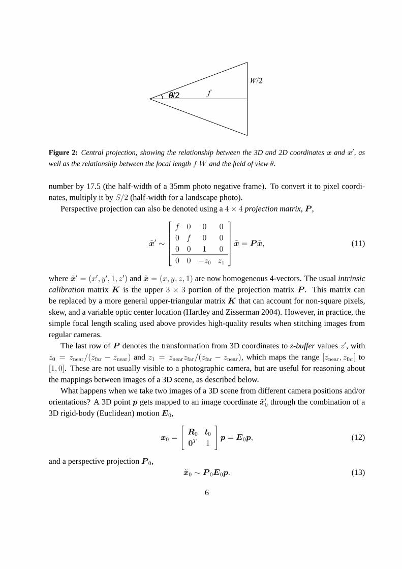
2004).The process ofcentral projectionmaps 3D coordinatesx = (x, y, z) to 2D coordinatesx′ =

(x′, y′, 1) through apinholeat the camera origin onto a 2D projection plane a distancef along thez axis,

x′ = fx

z, y′ = f

y

z, (9)

as shown in Figure 2. The relationship between the (unit-less) focal lengthf and the field of viewθ is given by

f−1 = tanθ

2or θ = 2 tan−1 1

f. (10)

To convert the focal lengthf to its more commonly used 35mm equivalent, multiply the above

5

���

����

Figure 2: Central projection, showing the relationship between the 3D and 2D coordinatesx and x′, as

well as the relationship between the focal lengthf W and the field of viewθ.

number by 17.5 (the half-width of a 35mm photo negative frame). To convert it to pixel coordi-nates, multiply it byS/2 (half-width for a landscape photo).

Perspective projection can also be denoted using a4× 4 projection matrix, P ,

x′ ∼

f 0 0 0

0 f 0 0

0 0 1 0

0 0 −z0 z1

x = P x, (11)

wherex′ = (x′, y′, 1, z′) andx = (x, y, z, 1) are now homogeneous 4-vectors. The usualintrinsic

calibration matrix K is the upper3 × 3 portion of the projection matrixP . This matrix canbe replaced by a more general upper-triangular matrixK that can account for non-square pixels,

skew, and a variable optic center location (Hartley and Zisserman 2004). However, in practice, thesimple focal length scaling used above provides high-quality results when stitching images from

regular cameras.The last row ofP denotes the transformation from 3D coordinates toz-buffervaluesz′, with

z0 = znear/(zfar − znear) andz1 = znearzfar/(zfar − znear), which maps the range[znear, zfar] to[1, 0]. These are not usually visible to a photographic camera, butare useful for reasoning about

the mappings between images of a 3D scene, as described below.What happens when we take two images of a 3D scene from different camera positions and/or

orientations? A 3D pointp gets mapped to an image coordinatex′0 through the combination of a

3D rigid-body (Euclidean) motionE0,

x0 =

R0 t0

0T 1

p = E0p, (12)

and a perspective projectionP 0,x0 ∼ P 0E0p. (13)

6

Assuming that we know the z-buffer valuez0 for a pixel in one image, we can map it back to the3D coordinatep using

p ∼ E−10 P−1

0 x0 (14)

and then project it into another image yielding

x1 ∼ P 1E1p = P 1E1E−10 P−1

0 x0 = M 01x0. (15)

Unfortunately, we do not usually have access to the depth coordinates of pixels in a regular

photographic image. However, for aplanar scene, we can replace the last row ofP 0 in (11) witha generalplane equation, n0 · p + d0 that maps points on the plane toz0 = 0 values. Then, if we

setz0 = 0, we can ignore the last column ofM 01 in (15) and also its last row, since we do not careabout the final z-buffer depth. The mapping equation (15) thus reduces to

x1 ∼ H01x0, (16)

whereH01 is a general3 × 3 homography matrix andx1 andx0 are now 2D homogeneous co-

ordinates (i.e., 3-vectors) (Szeliski 1994, Szeliski 1996).3 This justifies the use of the 8-parameterhomography as a general alignment model for mosaics of planar scenes (Mann and Picard 1994,Szeliski 1996).4

The more interesting case is when the camera undergoes pure rotation (which is equivalent toassuming all points are very far from the camera). Settingt0 = t1 = 0, we get the simplified3× 3

homographyH = K1R1R

−10 K−1, (17)

whereKk = diag(fk, fk, 1) is the simplified camera intrinsic matrix (Szeliski 1996). This can alsobe re-written as

x1

y1

f1

∼ R01

x0

y0

f0

, (18)

which shows the true simplicity of the mapping equations andmakes all of the motion parameters

explicit. Thus, instead of the general 8-parameter homography relating a pair of images, we getthe 3-, 4-, or 5-parameter3D rotationmotion models corresponding to the cases where the focal

lengthf is known, fixed, or variable (Szeliski and Shum 1997). Estimating the 3D rotation matrix

3For points off the reference plane, we get out-of-planeparallaxmotion, which is why this representation is oftencalled theplane plus parallaxrepresentation (Sawhney 1994, Szeliski and Coughlan 1994,Kumaret al.1994a).

4Note that for a single pair of images, the fact that a 3D plane is being viewed by a set of rigid cameras does notreduce the total number of degrees of freedom. However, for alarge collection of images taken of a planar surface(e.g., a whiteboard) from a calibrated camera, we could reduce the number of degrees of freedom per image from 8 to6 by assuming that the plane is at a canonical location (e.g.,z = 1).

7

(and optionally, focal length) associated with each image is intrinsically much more stable thanestimating a full 8-d.o.f. homography, which makes this themethod of choice for large-scale

consumer-level image stitching algorithms (Szeliski and Shum 1997, Shum and Szeliski 2000,Brown and Lowe 2003).

2.3 Cylindrical and spherical coordinates

An alternative to using homographies or 3D motions to align images is to first warp the images

into cylindrical coordinates and to then use a pure translational model to align them (Chen 1995).Unfortunately, This only works if the images are all taken with a level camera or with a known tilt

angle.Assume for now that the camera is in its canonical position, i.e., its rotation matrix is the

identity so that the optic axis is aligned with thez axis and they axis is aligned vertically. The 3Dray corresponding to an(x, y) pixel is therefore(x, y, f).

We wish to project this image onto acylindrical surfaceof unit radius (Szeliski 1994). Points

on this surface are parameterized by an angleθ and a heighth, with the 3D cylindrical coordinatescorresponding to(θ, h) given by

(sin θ, h, cos θ) ∝ (x, y, f). (19)

From this correspondence, we can compute the formula for thewarpedor mappedcoordinates

(Szeliski and Shum 1997),

x′ = sθ = s tan−1 x

f, (20)

y′ = sh = sy√

x2 + f 2, (21)

wheres is an arbitrary scaling factor (sometimes called theradiusof the cylinder) that can be setto s = f to minimize the distortion (scaling) near the center of the image.5 The inverse of thismapping equation is given by

x = f tan θ = f tanx′

s, (22)

y = h√

x2 + f 2 =y′

sf

√

1 + tan2 x′/s = fy′

ssec

x′

s. (23)

Images can also be projected onto aspherical surface(Szeliski and Shum 1997), which is use-

ful if the final panorama includes a full sphere or hemisphereof views, instead of just a cylindrical

5The scale can also be set to a larger or smaller value for the final compositing surface, depending on the desiredoutput panorama resolution—see§6.

8

strip. In this case, the sphere is parameterized by two angles (θ, φ), with 3D spherical coordinatesgiven by

(sin θ cosφ, sinφ, cos θ cosφ) ∝ (x, y, f). (24)

The correspondence between coordinates is now given by (Szeliski and Shum 1997)

x′ = sθ = s tan−1 x

f, (25)

y′ = sφ = s tan−1 y√x2 + f 2

, (26)

with the inverse given by

x = f tan θ = f tanx′

s, (27)

y =√

x2 + f 2 tanφ = tany′

sf

√

1 + tan2 x′/s = f tany′

ssec

x′

s. (28)

Note that it may be simpler to simply generate a scaled(x, y, z) direction from (19) followed by a

perspective division byz and a scaling byf .Cylindrical image stitching algorithms are most commonly used when the camera is known to

be level and only rotating around its vertical axis (Chen 1995). Under these conditions, imagesat different rotations are related by a pure horizontal translation.6 This makes it attractive as an

initial class project in an introductory computer vision course7, since the full complexity of theperspective alignment algorithm (§3.5 & §4.3) can be avoided.

Professional panoramic photographers sometimes also use apan-tilt head that makes it easy tocontrol the tilt and to stop at specificdetentsin the rotation angle.8 This not only ensures a uniformcoverage of the visual field with a desired amount of image overlap, but also makes it possible

to stitch the images using cylindrical or spherical coordinates and pure translations. In this case,pixel coordinates(x, y, f) must first be rotated using the known tilt and panning angles before

being projected into cylindrical or spherical coordinates(Chen 1995). Having a roughly knownpanning angle also makes it easier to compute the alignment,since the rough relative positioning

of all the input images is known ahead of time, enabling a reduced search range for alignment.One final coordinate mapping worth mentioning is thepolar mapping where the north pole lies

along the optic axis rather than the vertical axis,

(cos θ sinφ, sin θ sinφ, cosφ) = s (x, y, z). (29)

6Small vertical tilts can sometimes be compensated for with avertical translation.7//www.cs.washington.edu/homes/seitz/course/590SS/v4g.htm8See, e.g., //www.kaidan.com.

9

In this case, the mapping equations become

x′ = sφ cos θ = sx

rtan−1 r

z, (30)

y′ = sφ sin θ = sy

rtan−1 r

z, (31)

wherer =√x2 + y2 is theradial distancein the (x, y) plane andsφ plays a similar role in the

(x′, y′) plane. This mapping provides an attractive visualization surface for certain kinds of wide-

angle panoramas and is also a good model for the distortion induced byfisheyes lenses, as discussedbelow. Note how for small values of(x, y), the mapping equations reduces tox′ ≈ sx/z, which

suggests thats plays a role similar to the focal lengthf .

2.4 Lens distortions

When images are taken with wide-angle lenses, it is often necessary to modellens distortions

such asradial distortion. The radial distortion model says that coordinates in the observed images

are displaced away (barrel distortion) or towards (pincushiondistortion) the image center by anamount proportional to their radial distance. The simplestradial distortion models use low-order

polynomials, e.g.,

x′ = x(1 + κ1r2 + κ2r

4)

y′ = y(1 + κ1r2 + κ2r

4), (32)

wherer2 = x2 + y2 andκ1 andκ2 are called theradial distortion parameters(Brown 1971, Slama

1980).9 More complex distortion models also includetangential (decentering) distortions(Slama1980), but these are usually not necessary for consumer-level stitching.

A variety of techniques can be used to estimate the radial distortion parameters for a given

lens. One of the simplest and most useful is to take an image ofa scene with a lot of straight lines,especially lines aligned with and near the edges of the image. The radial distortion parameters can

then be adjusted until all of the lines in the image are straight, which is commonly called theplumb

line method(Brown 1971, Kang 2001, El-Melegy and Farag 2003).

Another approach is to use several overlapping images and tocombine the estimation of the ra-dial distortion parameters together with the image alignment process. Sawhney and Kumar (1999)

use a hierarchy of motion models (translation, affine, projective) in a coarse-to-fine strategy cou-pled with a quadratic radial distortion correction term. They use direct (intensity-based) mini-mization to compute the alignment. Stein (1997) uses a feature-based approach combined with

9Sometimes the relationship betweenx andx′ is expressed the other way around, i.e., using primed (final)coordi-nates on the right-hand side.

10

a general 3D motion model (and quadratic radial distortion), which requires more matches than aparallax-free rotational panorama but is potentially moregeneral.

Fisheye lenses require a different model than traditional polynomial models of radial distor-tion. Instead, fisheye lenses behave, to a first approximation, asequi-distanceprojectors of angles

away from the optic axis (Xiong and Turkowski 1997), which isthe same as thepolar projection

described by equations (29-31). Xiong and Turkowski (1997)describe how this model can beextended with the addition of an extra quadratic correctionin φ, and how the unknown parameters

(center of projection, scaling factors, etc.) can be estimated from a set of overlapping fisheyeimages using a direct (intensity-based) non-linear minimization algorithm.

3 Direct (pixel-based) alignment

Once we have chosen a suitable motion model to describe the alignment between a pair of images,we need to devise some method to estimate its parameters. Oneapproach is to shift or warp the

images relative to each other and to look at how much the pixels agree. Approaches that usepixel-to-pixel matching are often calleddirect methods, as opposed to thefeature-based methods

described in the next section.To use a direct method, a suitableerror metric must first be chosen to compare the images.

Once this has been established, a suitablesearchtechnique must be devised. The simplest tech-

nique is to exhaustively try all possible alignments, i.e.,to do afull search. In practice, this maybe too slow, sohierarchicalcoarse-to-fine techniques based on image pyramids have beendevel-

oped. Alternatively, Fourier transforms can be used to speed up the computation. To get sub-pixelprecision in the alignment,incrementalmethods based on a Taylor series expansion of the image

function are often used. These can also be applied toparametric motion models. Each of thesetechniques is described in more detail below.

3.1 Error metrics

The simplest way to establish an alignment between two images is to shift one image relative to

the other. Given atemplateimageI0(x) sampled at discrete pixel locations{xi = (xi, yi)}, wewish to find where it is located in imageI1(x). A least-squares solution to this problem is to find

the minimum of thesum of squared differences(SSD) function

ESSD(u) =∑

i

[I1(xi + u)− I0(xi)]2 =

∑

i

e2i , (33)

11

whereu = (u, v) is thedisplacementandei = I1(xi + u) − I0(xi) is called theresidual error

(or thedisplaced frame differencein the video coding literature).10 (We ignore for the moment the

possibility that parts ofI0 may lie outside the boundaries ofI1 or be otherwise not visible.)In general, the displacementu can be fractional, so a suitable interpolation function must be

applied to imageI1(x). In practice, a bilinear interpolant is often used, but bi-cubic interpolationmay yield slightly better results. Color images can be processed by summing differences across allthree color channels, although it is also possible to first transform the images into a different color

space or to only use the luminance (which is often done in video encoders).

Robust error metrics We can make the above error metric more robust to outliers by replacingthe squared error terms with a robust functionρ(ei) (Huber 1981, Hampelet al. 1986, Black and

Anandan 1996, Stewart 1999) to obtain

ESRD(u) =∑

i

ρ(I1(xi + u)− I0(xi)) =∑

i

ρ(ei). (34)

The robust normρ(e) is a function that grows less quickly than the quadratic penalty associated

with least squares. One such function, sometimes used in motion estimation for video codingbecause of its speed, is thesum of absolute differences(SAD) metric, i.e.,

ESAD(u) =∑

i

|I1(xi + u)− I0(xi)| =∑

i

|ei|. (35)

However, since this function is not differentiable at the origin, it is not well suited to gradient-descent approaches such as the ones presented in§3.4.

Instead, a smoothly varying function that is quadratic for small values but grows more slowly

away from the origin is often used. Black and Rangarajan (1996) discuss a variety of such func-tions, including theGeman-McClurefunction,

ρGM(x) =x2

1 + x2/a2, (36)

wherea is a constant that can be thought of as anoutlier threshold. An appropriate value for thethreshold can itself the derived using robust statistics (Huber 1981, Hampelet al.1986, Rousseeuwand Leroy 1987), e.g., by computing themedian of absolute differences, MAD = medi|ei|, and

multiplying by 1.4 to obtain a robust estimate of the standard deviation of the non-outlier noiseprocess.

10The usual justification for using least squares is that it is the optimal estimate with respect to Gaussian noise. Seethe discussion below on robust alternatives.

12

Spatially varying weights. The error metrics above ignore that fact that for a given alignment,some of the pixels being compared may lie outside the original image boundaries. Furthermore,

we may want to partially or completely downweight the contributions of certain pixels. For ex-ample, we may want to selectively “erase” some parts of an image from consideration, e.g., when

stitching a mosaic where unwanted foreground objects have been cut out. For applications such asbackground stabilization, we may want to downweight the middle part of the image, which oftencontains independently moving objects being tracked by thecamera.

All of these tasks can be accomplished by associating a spatially varying per-pixelweight

value with each of the two images being matched. The error metric then become theweighted(or

windowed) SSD function,

EWSSD(u) =∑

i

w0(x)w1(xi + u)[I1(xi + u)− I0(xi)]2, (37)

where the weighting functionsw0 andw1 are zero outside the valid ranges of the images.

If a large range of potential motions is allowed, the above metric can have a bias towardssmaller overlap solutions. To counteract this bias, the windowed SSD score can be divided by the

overlap areaA =

∑

i

w0(x)w1(xi + u) = (38)

to compute aper-pixel(or mean) squared pixel error. This square root of this quantity is the root

mean squaredintensity error

RMS =√

EWSSD/A (39)

often seen reported in comparative studies.

Bias and gain (exposure differences). Often, the two images being aligned were not taken with

the same exposure. A simple model of linear intensity variation between the two images is thebias

and gainmodel,

I1(x + u) = (1 + α)I0(x) + β, (40)

whereβ is thebiasandα is thegain (Lucas and Kanade 1981, Gennert 1988, Fuh and Maragos

1991, Bakeret al.2003b). The least squares formulation then becomes

EBG(u) =∑

i

[I1(xi + u)− (1 + α)I0(xi)− β]2 =∑

i

[αI0(xi) + β − ei]2. (41)

Rather than taking a simple squared difference between corresponding patches, it becomes neces-

sary to perform alinear regression, which is somewhat more costly. Note that for color images,it may be necessary to estimate a different bias and gain for each color channel to compensate forthe automaticcolor correctionperformed by some digital cameras.

13

A more general (spatially-varying non-parametric) model of intensity variation, which is com-puted as part of the registration process, is presented in (Jia and Tang 2003). This can be useful

for dealing with local variations such as thevignettingcaused by wide-angle lenses. It is alsopossible to pre-process the images before comparing their values, e.g., by using band-pass filtered

images (Burt and Adelson 1983, Bergenet al. 1992) or using other local transformations such ashistograms or rank transforms (Coxet al.1995, Zabih and Woodfill 1994).

Correlation. An alternative to taking intensity differences is to perform correlation, i.e., to max-

imize theproduct(or cross-correlation) of the two aligned images,

ECC(u) =∑

i

I0(xi)I1(xi + u). (42)

At first glance, this may appear to make bias and gain modelingunnecessary, since the images willprefer to line up regardless of their relative scales and offsets. However, this is actually not true. Ifa very bright patch exists inI1(x), the maximum product may actually lie in that area.

For this reason,normalized cross-correlationis more commonly used,

ENCC(u) =

∑

i[I0(xi)− I0] [I1(xi + u)− I1]√

∑

i[I0(xi)− I0]2[I1(xi + u)− I1]2, (43)

where

I0 =1

N

∑

i

I0(xi) (44)

I1 =1

N

∑

i

I1(xi + u) (45)

are themean imagesof the corresponding patches andN is the number of pixels in the patch. Thenormalized cross-correlation score is always guaranteed to be in the range[−1, 1], which makes it

easier to handle in some higher-level applications (such asdeciding which patches truly match).Note, however, that the NCC score is undefined if either of thetwo patches has zero variance (andin fact, its performance degrades for noisy low-contrast regions).

3.2 Hierarchical motion estimation

Now that we have defined an alignment cost function to optimize, how do we find its minimum?The simplest solution is to do afull searchover some range of shifts, using either integer or sub-

pixel steps. This is often the approach used forblock matchingin motion compensated video

compression, where a range of possible motions (say±16 pixels) is explored.11

11In stereo matching, an explicit search over all possible disparities (i.e., aplane sweep) is almost always performed,since the number of search hypotheses is much smaller due to the 1D nature of the potential displacements (Scharsteinand Szeliski 2002).

14

To accelerate this search process,hierarchical motion estimationis often used, where an imagepyramid is first constructed, and a search over a smaller number of discrete pixels (corresponding

to the same range of motion) is first performed at coarser levels (Quam 1984, Anandan 1989). Themotion estimate from one level of the pyramid can then be usedto initialize a smallerlocal search

at the next finer level. While this is not guaranteed to produce the same result as full search, itusually works almost as well and is much faster.

More formally, let

I(l)k (xj)← I

(l−1)k (2xj) (46)

be thedecimatedimage at levell obtained by subsampling (downsampling) a smoothed (pre-

filtered) version of the image at levell−1. At the coarsest level, we search for the best displacementu(l) that minimizes the difference between imagesI

(l)0 andI(l)

1 . This is usually done using a full

search over some range of displacementsu(l) ∈ 2−l[−S, S]2 (whereS is the desiredsearch range

at the finest (original) resolution level), optionally followed by the incremental refinement stepdescribed in§3.4.

Once a suitable motion vector has been estimated, it is used to predicta likely displacement

u(l−1) ← 2u(l) (47)

for the next finer level.12 The search over displacements is then repeated at the finer level overa much narrower range of displacements, sayu(l−1) ± 1, again optionally combined with an in-

cremental refinement step (Anandan 1989). A nice description of the whole process, extended toparametric motion estimation (§3.5), can be found in (Bergenet al.1992).

3.3 Fourier-based alignment

When the search range corresponds to a significant fraction of the larger image (as is the case inimage stitching), the hierarchical approach may not work that well, since it is often not possibleto coarsen the representation too much before significant features get blurred away. In this case, a

Fourier-based approach may be preferable.Fourier-based alignment relies on the fact that the Fouriertransform of a shifted signal has the

same magnitude as the original signal but linearly varying phase, i.e.,

F {I1(x + u)} = F {I1(x)} e−2πju·f = I1(f)e−2πju·f , (48)

12This doubling of displacements is only necessary if displacements are defined in integerpixel coordinates, whichis the usual case in the literature, e.g., (Bergenet al.1992). Ifnormalized device coordinates(§2) are used instead, thedisplacements (and search ranges) need not change from level to level, although the step sizes will need to be adjusted(to keep search steps of roughly one pixel).

15

wheref is the vector-valued frequency of the Fourier transform andwe use calligraphic notationI1(f) = F {I1(x)} to denote the Fourier transform of a signal (Oppenheimet al.1999, p. 57).

Another useful property of Fourier transforms is that convolution in the spatial domain corre-sponds to multiplication in the Fourier domain (Oppenheimet al.1999, p. 58).13 Thus, the Fourier

transform of the cross-correlation functionECC can be written as

F {ECC(u)} = F{

∑

i

I0(xi)I1(xi + u)

}

= F {I0(u)∗I1(u)} = I0(f )I∗1 (f), (49)

where

h(u) = f(u)∗g(u) =∑

i

f(xi)g(xi + u) (50)

is thecorrelation function, i.e., the convolution of one signal with the reverse of the other, andI∗1 (f ) is thecomplex conjugateof I1(f). (This is because convolution is defined as the summation

of one signal with the reverse of the other (Oppenheimet al.1999).)Thus, to efficiently evaluateECC over the range of all possible values ofu, we take the Fourier

transforms of both imagesI0(x) andI1(x), multiply both transforms together (after conjugatingthe second one), and take the inverse transform of the result. The Fast Fourier Transform algorithmcan compute the transform of anN ×M image in O(NM logNM) operations (Oppenheimet al.

1999). This can be significantly faster than the O(N2M2) operations required to do a full searchwhen the full range of image overlaps is considered.

While Fourier-based convolution is often used to accelerate the computation of image correla-tions, it can also be used to accelerate the sum of squared differences function (and its variants) as

well. Consider the SSD formula given in (33). Its Fourier transform can be written as

F {ESSD(u)} = F{

∑

i

[I1(xi + u)− I0(xi)]2

}

= δ(f)∑

i

[I20 (xi) + I2

1 (xi)]− 2I0(f )I∗1 (f).

(51)

Thus, the SSD function can be computed by taking twice the correlation function and subtractingit from the sum of the energies in the two images.

Windowed correlation. Unfortunately, the Fourier convolution theorem only applies when the

summation overxi is performed overall the pixels in both images, using a circular shift of theimage when accessing pixels outside the original boundaries. While this is acceptable for small

shifts and comparably sized images, it makes no sense when the images overlap by a small amountor one image is a small subset of the other.

13In fact, the Fourier shift property (48) derives from the convolution theorem by observing that shifting is equivalentto convolution with a displaced delta functionδ(x− u).

16

In that case, the cross-correlation function should be replaced with awindowed(weighted)cross-correlation function,

EWCC(u) =∑

i

w0(xi)I0(xi) w1(xi + u)I1(xi + u), (52)

= [w0(x)I20 (x)]∗[w1(x)I2

0 (x)] (53)

where the weighting functionsw0 andw1 are zero outside the valid ranges of the images, and bothimages are padded so that circular shifts return 0 values outside the original image boundaries.

A more interesting case is the computation of theweightedSSD function introduced in (37),

EWSSD(u) =∑

i

w0(x)w1(xi + u)[I1(xi + u)− I0(xi)]2 (54)

= w0(x)∗[w1(x)I21 (x)] + [w0(x)I2

0 (x)]∗w1(x)− 2[w0(x)I0(x)]∗[w1(x)I1(x)].

The Fourier transform of the resulting expression is therefore

F {EWSSD(u)} =W0(f)S∗1 (f ) + S0(f)W∗

1 (f )− 2I0(f)I∗1 (f ), (55)

whereW0 = F{w0(x)},I0 = F{w0(x)I0(x)},S0 = F{w0(x)I2

0 (x)}, and

W1 = F{w1(x)},I1 = F{w1(x)I1(x)},S1 = F{w1(x)I2

1 (x)}(56)

are the Fourier transforms of the weighting functions and theweightedsquared and original image

signals. Thus, for the cost of a few additional image multiplies and Fourier transforms, the correctwindowed SSD function can be computed.

The same kind of derivation can be applied to the bias-gain corrected sum of squared differencefunctionEBG. Again, Fourier transforms can be used to efficiently compute all of the correlationsneeded to perform the linear regression in the bias and gain parameters in order to estimate the

exposure-compensated difference for each potential shift.

Phase correlation. A variant of regular correlation (49) that is sometimes usedfor motion esti-mation isphase correlation(Kuglin and Hines 1975, Brown 1992). Here, the spectrum of the two

signals being matched iswhitenedby dividing each per-frequency product in (49) by the magni-tudes of the Fourier transforms

F {EPC(u)} =I0(f)I∗1 (f )

‖I0(f)‖‖I1(f )‖ (57)

before taking the final inverse Fourier transform. In the case of noiseless signals with perfect

(cyclic) shift, we haveI1(x + u) = I0(x), and hence from (48) we obtain

F {I1(x + u)} = I1(f )e−2πju·f = I0(f ) and

F {EPC(u)} = e−2πju·f . (58)

17

The output of phase correlation (under ideal conditions) istherefore a single spike (impulse) lo-cated at the correct value ofu, which (in principle) makes it easier to find the correct estimate.

Phase correlation has a reputation in some quarters of outperforming regular correlation, butthis behavior depends on the characteristics of the signalsand noise. If the original images are

contaminated by a noise signal in a narrow frequency band (e.g., low-frequency noise or peakedfrequency “hum”), the whitening process effectively de-emphasizes the noise in these regions.However, if the original signals have very low signal-to-noise ratio at some frequencies (say, two

blurry or low-textured images with lots of high-frequency noise), the whitening process can actu-ally decrease performance. To my knowledge, no systematic comparison of the two approaches

(together with other Fourier-based techniques such as windowed and/or bias-gain corrected differ-encing) has been performed, so this is an interesting area for further exploration.

Rotations and scale. While Fourier-based alignment is mostly used to estimate translationalshifts between images, it can, under certain limited conditions, also be used to estimate in-plane

rotations and scales. Consider two images that are relatedpurelyby rotation, i.e.,

I1(Rx) = I0(x). (59)

If we re-sample the images intopolar coordinates,

I0(r, θ) = I0(r cos θ, r sin θ) and I1(r, θ) = I1(r cos θ, r sin θ), (60)

we obtain

I1(r, θ + θ) = I0(r, θ). (61)

The desired rotation can then be estimated using an FFT shift-based technique.If the two images are also related by a scale,

I1(esRx) = I0(x), (62)

we can re-sample intolog-polar coordinates,

I0(s, θ) = I0(es cos θ, es sin θ) and I1(s, θ) = I1(e

s cos θ, es sin θ), (63)

to obtainI1(s+ s, θ + θ) = I0(s, θ). (64)

In this case, care must be taken to choose a suitable range ofs values that reasonably samples theoriginal image.

For images that are also translated by a small amount,

I1(esRx + t) = I0(x), (65)

18

De Castro and Morandi (1987) proposed an ingenious solutionthat uses several steps to estimatethe unknown parameters. First, both images are converted tothe Fourier domain, and only the

magnitudes of the transformed images are retained. In principle, the Fourier magnitude imagesare insensitive to translations in the image plane (although the usual caveats about border effects

apply). Next, the two magnitude images are aligned in rotation and scale using the polar or log-polar representations. Once rotation and scale are estimated, one of the images can be de-rotatedand scaled, and a regular translational algorithm can be applied to estimate the translational shift.

Unfortunately, this trick only applies when the images havelarge overlap (small translationalmotion). For more general motion of patches or images, the parametric motion estimator described

in §3.5 or the feature-based approaches described in§4 need to be used.

3.4 Incremental refinement

The techniques described up till now can estimate translational alignment to the nearest pixel (orpotentially fractional pixel if smaller search steps are used). In general, image stabilization and

stitching applications require much higher accuracies to obtain acceptable results.To obtain bettersub-pixelestimates, we can use one of several techniques (Tian and Huhns

1986). One possibility is to evaluate several discrete (integer or fractional) values of(u, v) aroundthe best value found so far, and tointerpolatethe matching score to find an analytic minimum.

A more commonly used approach, first proposed by Lucas and Kanade (1981), is to dogradient

descenton the SSD energy function (33), using a Taylor Series expansion of the image function,

ELK−SSD(u + ∆u) =∑

i

[I1(xi + u + ∆u)− I0(xi)]2

≈∑

i

[I1(xi + u) + J1(xi + u)∆u− I0(xi)]2 (66)

=∑

i

[J1(xi + u)∆u + ei]2, (67)

whereJ1(xi + u) = ∇I1(xi + u) = (

∂I1∂x

,∂I1∂y

)(xi + u) (68)

is theimage gradientatxi + u.14

The above least squares problem can be minimizing by solvingthe associatednormal equations

(Golub and Van Loan 1996),

A∆u = b (69)

14We follow the convention, commonly used in robotics and in (Baker and Matthews 2004), that derivatives withrespect to (column) vectors result in row vectors, so that fewer transposes are needed in the formulas.

19

whereA =

∑

i

JT1 (xi + u)J1(xi + u) (70)

andb = −

∑

i

eiJT1 (xi + u) (71)

are called theHessianandgradient-weighted residual vector, respectively. These matrices are also

often written as

A =

∑

I2x

∑

IxIy∑

IxIy∑

I2y

and b = −

∑

IxIt∑

IyIt

, (72)

where the subscripts inIx andIy denote spatial derivatives, andIt is called thetemporal derivative,which makes sense if we are computing instantaneous velocity in a video sequence.

The gradients required forJ1(xi + u) can be evaluated at the same time as the image warpsrequired to estimateI1(xi +u), and in fact are often computed as a side-product of image interpo-

lation. If efficiency is a concern, these gradients can be replaced by the gradients in thetemplate

image,

J1(xi + u) ≈ J0(x), (73)

since near the correct alignment, the template and displaced target images should look similar.This has the advantage of allowing the pre-computation of the Hessian and Jacobian images, which

can result in significant computational savings (Hager and Belhumeur 1998, Baker and Matthews2004).

The effectiveness of the above incremental update rule relies on the quality of the Taylor seriesapproximation. When far away from the true displacement (say 1-2 pixels), several iterations may

be needed. When started in the vicinity of the correct solution, only a few iterations usually suffice.A commonly used stopping criterion is to monitor the magnitude of the displacement correction‖u‖ and to stop when it drops below a certain threshold (say1/10th of a pixel). For larger motions,

it is usual to combine the incremental update rule with a hierarchical coarse-to-fine search strategy,as described in§3.2.

Conditioning and aperture problems. Sometimes, the inversion of the linear system (69) canbe poorly conditioned because of lack of two-dimensional texture in the patch being aligned. Acommonly occurring example of this is theaperture problem, first identified in some of the early

papers on optic flow (Horn and Schunck 1981) and then studied more extensively by Anandan(1989). Consider an image patch that consists of a slanted edge moving to the right. Only the

normal component of the velocity (displacement) can be reliably recovered in this case. This

20

manifests itself in (69) as arank-deficientmatrix A, i.e., one whose smaller eigenvalue is veryclose to zero.15

When equation (69) is solved, the component of the displacement along the edge is very poorlyconditioned and can result in wild guesses under small noiseperturbations. One way to mitigate

this problem is to add aprior (soft constraint) on the expected range of motions (Simoncelli et al.

1991, Bakeret al.2004). This can be accomplished by adding a small value to thediagonal ofA,which essentially biases the solution towards smaller∆u values that still (mostly) minimize the

squared error.16

However, the pure Gaussian model assumed when using a simple(fixed) quadratic prior, as in

(Simoncelliet al. 1991), does not always hold in practice, e.g., because of aliasing along strongedges (Triggs 2004). For this reason, it may be prudent to addsome small fraction (say 5%) of the

larger eigenvalue to the smaller one before doing the matrixinversion.17

Uncertainty modeling The reliability of a particular patch-based motion estimate can be cap-tured more formally with anuncertainty model. The simplest such model is acovariance matrix,

which captures the expected variance in the motion estimatein all possible directions. Under smallamounts of additive Gaussian noise, it can be shown that the covariance matrixΣu is proportional

to the inverse of the HessianA,Σu = σ2

nA−1, (74)

whereσ2n is the variance of the additive Gaussian noise (Anandan 1989, Matthieset al. 1989,

Szeliski 1989). For larger amounts of noise, the linearization performed by the Lucas-Kanadealgorithm in (67) is only approximate, so the above quantitybecomes theCramer-Rao lower bound

on the true covariance. Thus, the minimum and maximum eigenvalues of the HessianA can nowbe interpreted as the (scaled) inverse variances in the least-certain and most-certain directions of

motion.

Bias and gain, weighting, and robust error metrics. The Lucas-Kanade update rule can alsobe applied to the bias-gain equation (41) to obtain

ELK−BG(u + ∆u) =∑

i

[J1(xi + u)∆u + ei − αI0(xi)− β]2 (75)

15The matrixA is by construction always guaranteed to be symmetric positive semi-definite, i.e., it has real non-negative eigenvalues.

16In the terminology of Horn and Schunck (1981), one could say that thebrightness consistency constraintsare stilllargely satisfied.

17For2× 2 systems, the eigenvalues and eigenvectors have simple closed-form solutions.

21

(Lucas and Kanade 1981, Gennert 1988, Fuh and Maragos 1991, Bakeret al.2003b). The resulting4×4 system of equations in can be solved to simultaneously estimate the translational displacement

update∆u and the bias and gain parametersβ andα.18

A similar formulation can be derived for images (templates)that have alinear appearance

variation,I1(x + u) ≈ I0(x) +

∑

j

λjBj(x), (76)

where theBj(x) are thebasis imagesand theλj are the unknown coefficients (Hager and Bel-

humeur 1998, Bakeret al. 2003a, Bakeret al. 2003b). Potential linear appearance variations in-clude illumination changes (Hager and Belhumeur 1998) and small non-rigid deformations (Blackand Jepson 1998).

A weighted (windowed) version of the Lucas-Kanade algorithm is also possible,

ELK−WSSD(u + ∆u) =∑

i

w0(x)w1(xi + u)[J1(xi + u)∆u + ei]2. (77)

Note that here, in deriving the Lucas-Kanade update from theoriginal weighted SSD function(37), we have neglected taking the derivative ofw1(xi + u) weighting function with respect tou,

which is usually acceptable in practice, especially if the weighting function is a binary mask withrelatively few transitions.

Bakeret al. (2003a) only use thew0(x) term, which is reasonable if the two images have thesame extent and no (independent) cutouts in the overlap region. They also discuss the idea of mak-

ing the weighting proportional to∇I(x), which helps for very noisy images, where the gradientitself is noisy. Similar observation, formulated in terms of total least squares(Huffel and Vande-walle 1991), have been made by other researchers studying optic flow (motion) estimation (Weber

and Malik 1995). Lastly, Bakeret al. (2003a) show how evaluating (77) at just themost reliable

(highest gradient) pixels does not significantly reduce performance for large enough images, even

if only 5%-10% of the pixels are used. (This idea was originally proposed by Dellaert and Collins(1999), who use a more sophisticated selection criterion.)

The Lucas-Kanade incremental refinement step can also be applied to the robust error metricintroduced in§3.1,

ELK−SRD(u + ∆u) =∑

i

ρ(J1(xi + u)∆u + ei). (78)

We can take the derivative of this function w.r.t.u and set it to 0,

∑

i

ψ(ei)∂ei

∂u=

∑

i

ψ(ei)J1(x + u) = 0, (79)

18In practice, it may be possible to decouple the bias-gain andmotion update parameters, i.e., to solve two indepen-dent2× 2 systems, which is a little faster.

22

whereΨ(e) = ρ′(e) is the derivative ofρ. If we introduce a weight functionw(e) = Ψ(e)/e, wecan write this as

∑

i

w(ei)JT1 (x + u)[J1(xi + u)∆u + ei] = 0. (80)

This results in theIteratively Re-weighted Least Squaresalgorithm, which alternates between com-puting the weight functionsw(ei) and solving the above weighted least squares problem (Huber

1981, Stewart 1999). Alternative incremental robust leastsquares algorithms can be found in(Sawhney and Ayer 1996, Black and Anandan 1996, Black and Rangarajan 1996, Bakeret al.

2003a) and textbooks on robust statistics.

3.5 Parametric motion

Many image alignment tasks, for example image stitching with handheld cameras, require the useof more sophisticated motion models, as described in§2. Since these models typically have more

parameters than pure translation, a full search over the possible range of values is impractical.Instead, the incremental Lucas-Kanade algorithm can be generalized to parametric motion modelsand used in conjunction with a hierarchical search algorithm (Lucas and Kanade 1981, Rehg and

Witkin 1991, Fuh and Maragos 1991, Bergenet al.1992, Baker and Matthews 2004).For parametric motion, instead of using a single constant translation vectoru, we use a spatially

varyingmotion fieldor correspondence map, x′(x; p), parameterized by a low-dimensional vectorp, wherex′ can be any of the motion models presented in§2. The parametric incremental motion

update rule now becomes

ELK−PM(p + ∆p) =∑

i

[I1(x′(xi; p + ∆p))− I0(xi)]

2

≈∑

i

[I1(x′i) + J1(x

′i)∆p− I0(xi)]

2 (81)

=∑

i

[J1(x′i)∆p + ei]

2, (82)

where the Jacobian is now

J1(x′i) =

∂I1∂p

= ∇I1(x′i)∂x′

∂p(xi) (83)

i.e., the product of the image gradient∇I1 with the Jacobian of correspondence field,Jx′ =

∂x′/∂p.

Table 2 shows the motion JacobiansJx′ for the 2D planar transformations introduced in§2.Note how I have re-parameterized the motion matrices so thatthey are always the identity at the

origin p = 0. This will become useful below, when we talk about the compositional and inversecompositional algorithms. (It also makes it easier to impose priors on the motions.)

23

Transform Matrix Parameters JacobianJx′

translation

1 0 tx0 1 ty

(tx, ty)

1 0

0 1

Euclidean

cθ −sθ txsθ cθ ty

(tx, ty, θ)

1 0 −sθx− cθy0 1 cθx− sθy

similarity

1 + a −b txb 1 + a ty

(tx, ty, a, b)

1 0 x −y0 1 y x

affine

1 + a00 a01 txa10 1 + a11 ty

(tx, ty, a00, a01, a10, a11)

1 0 x y 0 0

0 1 0 0 x y

projective

1 + h00 h01 h02

h10 1 + h11 h12

h20 h21 1

(h00, . . . , h21)(see text)

Table 2: Jacobians of the 2D coordinate transformations.

The derivatives in Table 2 are all fairly straightforward, except for the projective 2-D motion(homography), which requires a per-pixel division to evaluate, c.f. (8), re-written here in its new

parametric form as

x′ =(1 + h00)x+ h01y + h02

h20x+ h21y + 1and y′ =

h10x+ (1 + h11)y + h12

h20x+ h21y + 1. (84)

The Jacobian is therefore

Jx′ =∂x′

∂p=

1

D

x y 1 0 0 0 −x′x −x′y0 0 0 x y 1 −y′x −y′y

, (85)

whereD is the denominator in (84), which depends on the current parameter settings (as dox′ andy′).

For parametric motion, theHessianandgradient-weighted residual vectorbecome

A =∑

i

JTx′(xi)[∇IT

1 (x′i)∇I1(x′

i)]Jx′(xi) (86)

andb = −

∑

i

JTx′(xi)[ei∇IT

1 (x′i)]. (87)

Note how the expressions inside the square brackets are the same ones evaluated for the simplertranslational motion case (70–71).

24

Patch-based approximation. The computation of the Hessian and residual vectors for paramet-ric motion can be significantly more expensive than for the translational case. For parametric

motion withn parameters andN pixels, the accumulation ofA andb takes O(n2N) operations(Baker and Matthews 2004). One way to reduce this by a significant amount is to divide the image

up into smaller sub-blocks (patches) and to only accumulatethe simpler2× 2 quantities inside thesquare brackets at the pixel level (Shum and Szeliski 2000).The full Hessian and residual can thenbe re-written as

A =∑

j

JTx′(xj)[

∑

i∈Pj

∇IT1 (x′

i)∇I1(x′i)]Jx′(xj) (88)

and

b = −∑

j

JTx′(xj)[

∑

i∈Pj

ei∇IT1 (x′

i)], (89)

wherexj is thecenterof each patchPj . This is equivalent to replacing the true motion Jacobianwith a piecewise-constant approximation. In practice, this works quite well (Szeliski and Shum

1997). The relationship of this approximation to feature-based registration is discussed in§4.4.

Compositional approach For a complex parametric motion such as a homography, the compu-

tation of the motion Jacobian becomes complicated, and may involve a per-pixel division. Szeliskiand Shum (1997) observed that this can be simplified by first warping the target imageI1 accordingto the current motion estimatex′(x; p),

I1(x) = I1(x′(x; p)), (90)

and then comparing thiswarpedimage against the templateI0(x),

ELK−SS(∆p) =∑

i

[I1(x(xi; ∆p))− I0(xi)]2

≈∑

i

[J1(xi)∆p + ei]2 (91)

=∑

i

[∇I1(xi)Jx(xi)∆p + ei]2. (92)

Note that since the two images are assumed to be fairly similar, only an incrementalparametricmotion is required, i.e., the incremental motion can be evaluated aroundp = 0, which can lead

to considerable simplifications. For example, the Jacobianof the planar projective transform (84)now becomes

Jx =∂x

∂p

∣

∣

∣

∣

∣

p=0

=

x y 1 0 0 0 −x2 −xy0 0 0 x y 1 −xy −y2

. (93)

Once the incremental motionx has been computed, it can beprependedto the previously estimatedmotion, which is easy to do for motions represented with transformation matrices, such as those

25

given in Tables 1–2. Baker and Matthews (2004) call this theforward compositionalalgorithm,since the target image is being re-warped, and the final motion estimates are being composed.

If the appearance of the warped and template images is similar enough, we can replace thegradient ofI1(x) with the gradient ofI0(x), as suggested previously in (73). This has potentially

a big advantage, in that it allows the pre-computation (and inversion) of the Hessian matrixAgiven in (86). The residual vectorb (87) can also be partially precomputed, i.e., thesteepest

descentimages∇I0(x)Jx(x) can precomputed and stored for later multiplication with thee(x) =

I1(x) − I0(x) error images (Baker and Matthews 2004). This idea was first suggested by Hagerand Belhumeur (1998) in what Baker and Matthews (2004) call aforward additivescheme.

Baker and Matthews (2004) introduce one more variant they call the inverse compositional

algorithm. Rather than (conceptually) re-warping the warped target imageI1(x), they instead

warp the template imageI0(x) and minimize

ELK−BM(∆p) =∑

i

[I1(xi)− I0(x(xi; ∆p))]2

≈∑

i

[∇I0(xi)Jx(xi)∆p− ei]2. (94)

This is identical to the forward warped algorithm (92) with the gradients∇I1(x) replaced by thegradients∇I0(x), except for the sign ofei. The resulting update∆p is thenegativeof the onecomputed by the modified (92), and hence theinverseof the incremental transformation must be

prepended to the current transform. Because the inverse compositional algorithm has the potentialof pre-computing the inverse Hessian and the steepest descent images, this makes it the preferred

approach of those surveyed in (Baker and Matthews 2004).Baker and Matthews (2004) also discusses the advantage of using Gauss-Newton iteration (i.e.,

the first order expansion of the least squares, as above) vs. other approaches such as steepest de-scent andLevenberg-Marquardt. Subsequent parts of the series (Bakeret al. 2003a, Bakeret al.

2003b, Bakeret al. 2004) discuss more advanced topics such as per-pixel weighting, pixel selec-tion for efficiency, a more in-depth discussion of robust metrics and algorithms, linear appearancevariations, and priors on parameters. They make for invaluable reading for anyone interested in

implementing a highly tuned implementation of incrementalimage registration.

4 Feature-based registration

As I mentioned earlier, directly matching pixel intensities is just one possible approach to image

registration. The other major approach is to first extract distinctivefeaturesfrom each image, tomatch individual features to establish a global correspondence, and to then estimate the geometric

transformation between the images. This kind of approach has been used since the early days of

26

stereo matching (Hannah 1974, Hannah 1988) and has more recently gained popularity for imagestitching applications (Zoghlamiet al.1997, Capel and Zisserman 1998, Cham and Cipolla 1998,

Badraet al.1998, McLauchlan and Jaenicke 2002, Brown and Lowe 2003).In this section, I review methods for detecting distinctivepoints, for matching them, and for

computing the image registration, including the 3D rotation model introduced in§2.2. I also dis-cuss the relative advantages and disadvantages of direct and feature-based approaches.

4.1 Interest point detectors

As we saw in§3.4, the reliability of a motion estimate depends most critically on the size of the

smallest eigenvalue of the Lucas and Kanade (1981) Hessian matrix, λ0 (Anandan 1989). Thismakes this a reasonable candidate for finding points in the image that can be matched with high

accuracy. (Older terminology in this field talked about “corner-like” features, but the modern usageis interest points.) Indeed, Shi and Tomasi (1994) propose using this quantityto findgood features

to track, and then use a combination of translational and affine-based patch alignment to track such

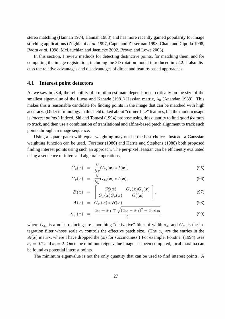
points through an image sequence.Using a square patch with equal weighting may not be the best choice. Instead, a Gaussian

weighting function can be used. Forstner (1986) and Harrisand Stephens (1988) both proposedfinding interest points using such an approach. The per-pixel Hessian can be efficiently evaluated

using a sequence of filters and algebraic operations,

Gx(x) =∂

∂xGσd

(x) ∗ I(x), (95)

Gy(x) =∂

∂yGσd

(x) ∗ I(x), (96)

B(x) =

G2x(x) Gx(x)Gy(x)

Gx(x)Gy(x) G2y(x)

, (97)

A(x) = Gσi(x) ∗B(x) (98)

λ0,1(x) =a00 + a11 ∓

√

(a00 − a11)2 + a01a10

2, (99)

whereGσdis a noise-reducing pre-smoothing “derivative” filter of width σd, andGσi

is the in-

tegration filter whose scaleσi controls the effective patch size. (Theaij are the entries in theA(x) matrix, where I have dropped the(x) for succinctness.) For example, Forstner (1994) uses

σd = 0.7 andσi = 2. Once the minimum eigenvalue image has been computed, localmaxima canbe found as potential interest points.

The minimum eigenvalue is not the only quantity that can be used to find interest points. A

27

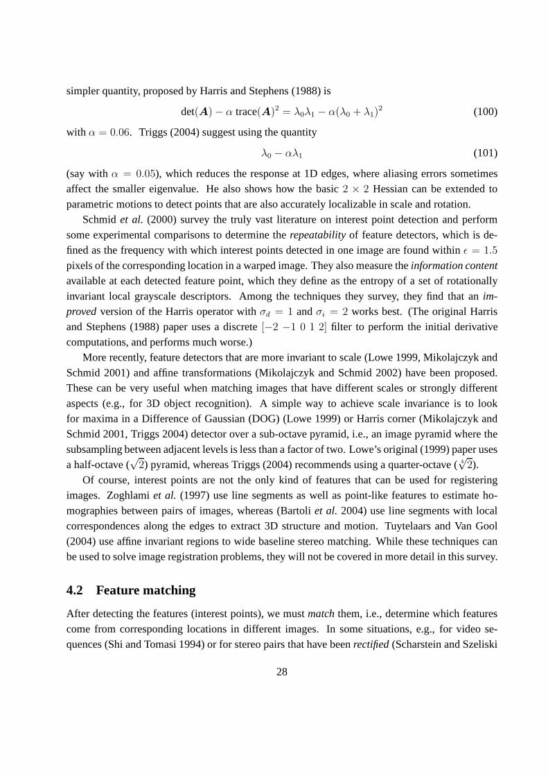
simpler quantity, proposed by Harris and Stephens (1988) is

det(A)− α trace(A)2 = λ0λ1 − α(λ0 + λ1)2 (100)

with α = 0.06. Triggs (2004) suggest using the quantity

λ0 − αλ1 (101)

(say withα = 0.05), which reduces the response at 1D edges, where aliasing errors sometimesaffect the smaller eigenvalue. He also shows how the basic2 × 2 Hessian can be extended to

parametric motions to detect points that are also accurately localizable in scale and rotation.Schmidet al. (2000) survey the truly vast literature on interest point detection and perform

some experimental comparisons to determine therepeatabilityof feature detectors, which is de-fined as the frequency with which interest points detected inone image are found withinε = 1.5

pixels of the corresponding location in a warped image. Theyalso measure theinformation content

available at each detected feature point, which they define as the entropy of a set of rotationally

invariant local grayscale descriptors. Among the techniques they survey, they find that anim-

provedversion of the Harris operator withσd = 1 andσi = 2 works best. (The original Harrisand Stephens (1988) paper uses a discrete[−2 −1 0 1 2] filter to perform the initial derivative

computations, and performs much worse.)More recently, feature detectors that are more invariant toscale (Lowe 1999, Mikolajczyk and

Schmid 2001) and affine transformations (Mikolajczyk and Schmid 2002) have been proposed.These can be very useful when matching images that have different scales or strongly different

aspects (e.g., for 3D object recognition). A simple way to achieve scale invariance is to lookfor maxima in a Difference of Gaussian (DOG) (Lowe 1999) or Harris corner (Mikolajczyk andSchmid 2001, Triggs 2004) detector over a sub-octave pyramid, i.e., an image pyramid where the

subsampling between adjacent levels is less than a factor oftwo. Lowe’s original (1999) paper usesa half-octave (

√2) pyramid, whereas Triggs (2004) recommends using a quarter-octave (4

√2).

Of course, interest points are not the only kind of features that can be used for registeringimages. Zoghlamiet al. (1997) use line segments as well as point-like features to estimate ho-

mographies between pairs of images, whereas (Bartoliet al. 2004) use line segments with localcorrespondences along the edges to extract 3D structure andmotion. Tuytelaars and Van Gool

(2004) use affine invariant regions to wide baseline stereo matching. While these techniques canbe used to solve image registration problems, they will not be covered in more detail in this survey.

4.2 Feature matching

After detecting the features (interest points), we mustmatchthem, i.e., determine which features

come from corresponding locations in different images. In some situations, e.g., for video se-quences (Shi and Tomasi 1994) or for stereo pairs that have beenrectified(Scharstein and Szeliski

28

2002), the local motion around each feature point may be mostly translational. In this case, the er-ror metrics introduced in§3.1 such asESSD orENCC can be used to directly compare the intensities

in small patches around each feature point. (The comparative study by Mikolajczyk and Schmid(2003) discussed below uses cross-correlation.) Because feature points may not be exactly located,

a more accurate matching score can be computed by performingincremental motion refinement asdescribed in§3.4, but this can be time consuming.

If features are being tracked over longer image sequences, their appearance can undergo larger

changes. In this case, it makes sense to compare appearancesusing anaffinemotion model. Shiand Tomasi (1994) compare patches using a translational model between neighboring frames, and

use the location estimate produced by this step to initialize an affine registration between the patchin the current frame and the base frame where a feature was first detected. In fact, features are

only detected infrequently, i.e., only in region where tracking has failed. In the usual case, an areaaround the currentpredictedlocation of the feature is searched with an incremental registration

algorithm. This kind of algorithm is adetect then trackapproach, since detection occurs infre-quently. It is appropriate for video sequences where the expected locations of feature points can bereasonably well predicted.

For larger motions, or for matching collections of images where the geometric relationshipbetween them is unknown (Schaffalitzky and Zisserman 2002,Brown and Lowe 2003), adetect

then matchapproach in which feature points are first detected in all images is more appropriate.Because the features can appear in different orientations and scale, a moreview invariantkind

of representation must be used. Mikolajczyk and Schmid (2003) review some recently developedview-invariant local image descriptors and experimentally compare their performance.

The simplest method to compensate for in-plane rotations isto find adominant orientation

at each feature point location before sampling the patch or otherwise computing the descriptor.Mikolajczyk and Schmid (2003) use the direction of the average gradient orientation, computed

within a small neighborhood of each feature point. The descriptor can be made invariant to scale byonly selecting feature points that are local maxima in scalespace, as discussed in§4.1. Making the

descriptors invariant to affine deformations (stretch, squash, skew) is even harder; Mikolajczyk andSchmid (2002) use the local moment matrix around a feature point to define a canonical frame.

Among the local descriptors that Mikolajczyk and Schmid (2003) compared, David Lowe’s(1999) Scale Invariant Feature Transform (SIFT) and Freeman and Adelson’s (1991) steerablefilters performed the best. SIFT features are computed by first estimating a local orientation using

a histogram of the local gradient orientations, which is potentially more accurate than just theaverage orientation. Once the local frame has been established, gradients are copied into different

orientation planes, and blurred resampled versions of these images as used as the features. Thisprovides the descriptor with some insensitivity to small feature localization errors and geometric

distortions (Lowe 1999).

29

Steerable filters are combinations of derivative of Gaussian filters that permit the rapid com-putation of even and odd (symmetric and anti-symmetric) edge-like and corner-like features at all

possible orientations (Freeman and Adelson 1991). Becausethey use reasonably broad Gaussians,they too are somewhat insensitive to localization and orientation errors. In their experimental

comparisons, Mikolajczyk and Schmid (2003) found that SIFTfeatures generally performed best,followed by steerable filters, and then cross-correlation (which could potentially be improved withan incremental refinement of location and pose). Differential invariants, whose descriptors are

insensitive to changes in orientation by design, did not do as well.

Rapid indexing and matching. The simplest way to find all corresponding feature points inan image pair is to compare all features in one image against all features in the other, using one

the local descriptors described above. Unfortunately, this is quadratic in the expected number offeatures, which makes it impractical for some applications.

More efficient matching algorithms can be devised using different kinds ofindexing schemes.Many of these are based on the idea of finding nearest neighbors in high-dimensional spaces. For

example, Nene and Nayar (1997) developed a technique they call slicing that uses a series of 1Dbinary searches to efficiently cull down a list of candidate points that lie within a hypercube of thequery point. They also provide a nice review of previous workin this area, including spatial data

structures such ask-d trees (Samet 1989). Beis and Lowe (1997) propose a Best-Bin-First (BBF)algorithm, which uses a modified search ordering for ak-d tree algorithm so that bins in feature

space are searched in the order of their closest distance from query location. Shakhnarovichet

al. (2003) extend a previously developed technique calledlocality-sensitive hashing, which uses

unions of independently computed hashing functions, to be more sensitive to the distribution ofpoints in parameter space, which they callparameter-sensitive hashing. Despite all of this promis-

ing work, the rapid computation of image feature correspondences is far from being a solvedproblem.

RANSAC and LMS. Once an initial set of feature correspondences has been computed, weneed to find a set that is will produce a high-accuracy alignment. One possible approach is to

simply compute a least squares estimate, or to use a robustified (iteratively re-weighted) versionof least squares, as discussed below (§4.3). However, in many cases, it is better to first find a good

starting set ofinlier correspondences, i.e., points that are all consistent withsome particular motionestimate.19

Two widely used solution to this problem are called Random SAmple Consensus, or RANSACfor short (Fischler and Bolles 1981) andleast median of squares(LMS) (Rousseeuw 1984). Both

19For direct estimation methods, hierarchical (coarse-to-fine) techniques are often used to lock onto thedominantmotionin a scene (Bergenet al.1992).

30

techniques start by selecting (at random) a subset ofk correspondences, which is then used tocompute a motion estimatep, as described in§4.3. Theresidualsof the full set of correspondences

are then computed asri = x′

i(xi; p)− x′i, (102)

where x′i are theestimated(mapped) locations, andx′

i are the sensed (detected) feature pointlocations.

The RANSAC technique then counts the number ofinliers that are withinε of their detected

location, i.e., whose‖ri‖ ≤ ε. (The ε value is application dependent, but often is around 1-3pixels.) Least median of squares finds the median value of the‖ri‖ values.

The random selection process is repeatedS times, and the sample set with largest numberof inliers (or with the smallest median residual) is kept as the final solution. Either the initial

parameter guessp or the full set of computed inliers is then passed on to the next data fitting stage.To ensure that the random sampling has a good chance of findinga true set of inliers, a sufficient

number of trialsS must be tried. Letp be the probability that any given correspondence is valid,

andP be the total probability of success afterS trials. The likelihood in one trial that allk randomsamples are inliers ispk. Therefore, the likelihood thatS such trials will all fail is

1− P = (1− pk)S (103)

and the required minimum number of trials is

S =log(1− P )

log(1− pk). (104)

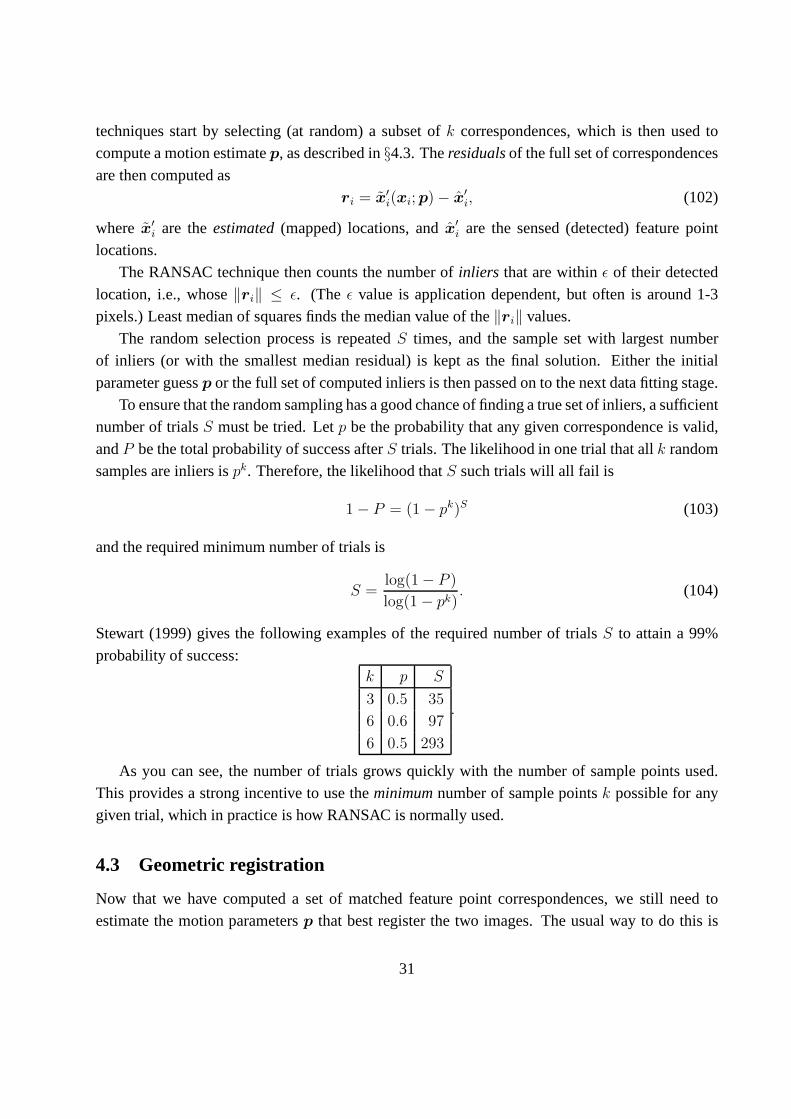
Stewart (1999) gives the following examples of the requirednumber of trialsS to attain a 99%

probability of success:k p S

3 0.5 35

6 0.6 97

6 0.5 293

.

As you can see, the number of trials grows quickly with the number of sample points used.This provides a strong incentive to use theminimumnumber of sample pointsk possible for anygiven trial, which in practice is how RANSAC is normally used.

4.3 Geometric registration

Now that we have computed a set of matched feature point correspondences, we still need toestimate the motion parametersp that best register the two images. The usual way to do this is

31

to use least squares, i.e., to minimize the sum of squared residuals given by (102). Many of themotion models presented in§2, i.e., translation, similarity, and affine, have alinear relationship

between the motion and the unknown parametersp.20 In this case, a simple linear regression (leastsquares) using normal equationsAp = b works well.21

For non-linearmeasurement equations such as the homography given in (84),rewritten here(for convenience) as

x′ =(1 + h00)x+ h01y + h02

h20x+ h21y + 1and y′ =

h10x+ (1 + h11)y + h12

h20x+ h21y + 1, (105)

a different solution is required. An initial guess for the 8 unknowns{h00, . . . , h21} can be obtainedby multiplying both sides of the equations through by the denominator, which yields the linear set

of equations,

x′ − xy′ − y

=

x y 1 0 0 0 −x′x −x′y0 0 0 x y 1 −y′x −y′y

h00

...

h21

. (106)

However, this is not optimal from a statistical point of view, since the denominator can vary quite

a bit from point to point.One way to compensate for this is tore-weighteach equation by the inverse of current estimate

of the denominator,D,

1

D

x′ − xy′ − y

=1

D

x y 1 0 0 0 −x′x −x′y0 0 0 x y 1 −y′x −y′y

h00

...h21

. (107)

While this may at first seem to be the exact same set of equations as (106), since least squares is

being used to solve the over-determined set of equations, the weightingsdo matter, and result in adifferent set of normal equations that perform better in practice (with noisy data).

The most principled way to do the estimation, however, is to directly minimize the squaredresidual equations (102) using the Gauss-Newton approximation, i.e., performing a first-order Tay-

lor series expansion inp, which yields,

x′i − x′

i(xi; p) = Jx′∆p (108)

or

x′ − x′y′ − y′

=1

D

x y 1 0 0 0 −x′x −x′y0 0 0 x y 1 −y′x −y′y

∆h00

...∆h21

. (109)

202-D Euclidean motion can be estimated with a linear algorithm by first estimating the cosine and sine entriesindependently, and then normalizing them so their magnitude is 1.

21For poorly conditioned problems, it is sometimes preferable to use QR decomposition on the set of linear equationsinstead of normal equation (Golub and Van Loan 1996). However, such conditions rarely arise in image registration.

32

While this looks similar to (107), it differs in two important respects. First, the left hand sideconsists of unweightedprediction errorsrather than pixel displacements, and the solution vector

is a perturbationto the parameter vectorp. Second the quantities insideJx′ involve predicted

feature locations(x′, y′) instead ofsensedfeature locations(x′, y′). Both of these are subtle, and

yet they lead to an algorithm that, when combined with properchecking for downhill steps (as inthe Levenberg-Marquardt algorithm), will converge to a minimum. (Iterating the (107) equationsis not guaranteed to do so, since it is not minimizing a well-defined energy function.)

Rotational panoramas. How to update the rotation matrix given by (17) using the incrementalupdate first described in (Szeliski and Shum 1997, Shum and Szeliski 2000).

Need to describe my preferred representation for rotations, which is quaternions.

Uncertainty weighting. How to incorporate a2 × 2 uncertainty matrix, and how this relates todirect methods.

Robust regression. How to apply an M-estimator, as given inERSD, but directly to the position

residuals. Why Gauss-Newton iteration (i.e., iterativelyre-weighted least squares) is required.

4.4 Direct vs. feature-based

How I used to be in the direct matching camp (Triggset al.2000), but since reading (Brown andLowe 2003) and working with feature based methods, I think they are preferable for large-motion

stitching applications. However, combining these with a patch-based refinement can lead to higheraccuracy and potentially better de-ghosting.

5 Global registration

How to take pairwise results and extend to full mosaic (Szeliski and Shum 1997, Shum and Szeliski2000, Hsu and Sawhney 1998, Sawhney and Kumar 1999, Coorg andTeller 2000)

5.1 Bundle adjustment

Basically taken from (Shum and Szeliski 2000), but with reference to general bundle adjustment

algorithms (Triggset al.1999)

33

5.2 Parallax removal

In (Shum and Szeliski 2000), this is calledlocal alignment

de-ghosting, i.e., parallax and lens distortion removal (Shum and Szeliski 2000) (uses interpo-lated block-based flow + bundle adjuster)

compensating for motion (Kanget al.2003)3D parallax: plane+parallax (Kumaret al.1994b, Sawhney 1994, Szeliski and Coughlan 1994,

Szeliski and Coughlan 1997) 3-D parallax (Kumaret al.1995, Szeliski and Kang 1995),MPPS (Uyttendaeleet al.2004, Kanget al.2004)

If we know the camera motion, then can use a 3D reconstruction. Place the camera in-between,and re-generate new locations.

5.3 Recognizing panoramas

First rapidly discover which pairs have sufficient overlap to be good candidates (Brown and Lowe

2003). Then, find connected components in this graph.In practice, may be erroneous matches, need a way to “back out” or make the process more

robust.Show example where solution is ambiguous: Doorway w/ tree orcathedral with windows vs.

moving persons

6 Compositing

Once we have registered all of the input images with respect to each other, we need to decide howto produce the final stitched (mosaic) image. This involves selecting a final compositing surface

(flat, cylindrical, spherical, etc.) and view (reference image). It also involves selecting which pixelscontribute to the final composite and how to optimally blend these pixels to minimize the visible

seams, blur, and ghosting.In this section, I review techniques that address these problems, namely compositing surface

parameterization, pixel/seam selection, blending, and exposure compensation. My emphasis ison fully automatedapproaches to the problem. Since the creation of high-quality panoramas andcomposites is as much anartistic endeavor as a computational one, various interactive toolshave

been developed to assist this process, e.g., (Agarwalaet al. 2004, Li et al. 2004a, Rotheret al.

2004), which I will not cover, except where they provide automated solutions to our problems.

34

6.1 Choosing a compositing surface

The first choice to be made is how to represent the final image. If only a few images are stitched

together, a natural approach is to select one of the images asthe referenceand to then warp allof the other images into the reference coordinate system. The resulting composite is called aflat

panorama, since the projection onto the final surface is still a perspective projection, and hencestraight lines remain straight (which is usually a desirable attribute).

For larger fields of view, however, we cannot maintain a flat representation without excessivelystretching pixels near the border of the image. (In practice, flat panoramas start to look severely dis-

torted once the field of view exceeds90◦ or so.) The usual choice for compositing larger panoramasis to use a cylindrical (Szeliski 1994, Chen 1995) or spherical (Szeliski and Shum 1997) projection,as described in§2.3. In fact, any surface used forenvironment mappingin computer graphics can

be used, including acube mapthat represents the full viewing sphere with the six square faces ofa box (Greene 1986, Szeliski and Shum 1997). Cartographers have also developed a number of

alternative methods for representing the globe .The choice of parameterization is somewhat application dependent, and involves a tradeoff

between keeping the local appearance undistorted (e.g., keeping straight lines straight) and provid-ing a reasonably uniform sampling of the environment. Automatically making this selection and

smoothly transitioning between representations based on the extent of the panorama is an interest-ing topic for future research.

View selection. Once we have chosen the output parameterization, we still need to determine

which part of the scene will becenteredin the final view. As mentioned above, for a flat composite,we can choose one of the images as a reference. Often, a reasonable choice is the one that isgeometrically most central. For example, for rotational panoramas represented as a collection

of 3D rotation matrices, we can choose the image whosez-axis is closest to the averagez-axis(assuming a reasonable field of view). Alternatively, we canuse the averagez-axis (or quaternion,

but this is trickier) to define the reference rotation.For larger (e.g., cylindrical or spherical) panoramas, we can still use the same heuristic if a

subset of the viewing sphere has been imaged. If the case of full 360◦ panoramas, a better choicemight be to choose the middle image from the sequence of inputs, or sometimes the first image,assuming this contains the object of greatest interest. In all of these cases, having the user control

the final view is often highly desirable. If the “up vector” computation described in§?? is workingcorrectly, this can be as simple as panning over the image or setting a vertical “center line” for the

final panorama.

35

Coordinate transformations. Once we have selected the parameterization and reference view,we still need to compute the mappings between the input and output pixels coordinates.

If the final compositing surface is flat (e.g., a single plane or the face of a cube map) and theinput images have no radial distortion, the coordinate transformation is the simple homography

described by (17). This kind of warping can be performed in graphics hardware by appropriatelysetting texture mapping coordinates and rendering a singlequadrilateral.

If the final composite surface has some other analytic form (e.g., cylindrical or spherical), we

need to convert every pixel in the final panorama into a viewing ray (3D point) and then mapit back into each image according to the projection (and optionally radial distortion) equations.

This process can be made more efficient by precomputing some lookup tables, e.g., the partialtrigonometric functions needed to map cylindrical or spherical coordinates to 3D coordinates, or

the radial distortion field at each pixel. It is also be possible to accelerate this process by computingexact pixel mappings on a coarser grid and then interpolating these values. An efficient way to

roughly know which portions of the final panorama are coveredby which input images can also behelpful.

When the final compositing surface is a texture-mapped polyhedron, a slightly more sophis-

ticated algorithm must be used (Szeliski and Shum 1997). Notonly do the 3D and texture mapcoordinates have to be properly handled, but a small amount of overdrawoutside of the triangle

footprints in the texture map is necessary, to ensure that the texture pixels being interpolated during3D rendering have valid values.

Sampling issues. While the above computations can yield the correct (fractional) pixel addresses

in each input image, we still need to pay attention to sampling issues. For example, if the finalpanorama has a lower resolution than the input images, pre-filtering the input images is neces-

sary to avoid aliasing. These issues have been extensively studied in both the image processingand computer graphics communities. The basic problem is to compute the appropriate pre-filter,which depends on the distance (and arrangement) between neighboring samples in a source image.

Various approximate solutions, such as MIP mapping (Williams 1983) or elliptically weightedGaussian averaging (Greene and Heckbert 1986) have been developed in the graphics commu-

nity. For highest visual quality, a higher order (e.g., cubic) interpolator combined with a spatiallyadaptive pre-filter may be necessary (Wanget al.2001). Under certain conditions, it may also be

possible to produce images with a higher resolution than theinput images using a process calledsuper-resolution(§7).

36

Figure 3: Final composites computed by a variety of algorithms: (a) average, (b) median, (c) feathered

average, (d)p-normp =?, (e) Vornoi, (f) weighted ROD vertex cover with feathering,(g) graph cut seams,

(h) graph cut seams with Poisson blending.

6.2 Pixel selection and weighting

Once the source pixels have been mapped onto the final composite surface, we must still decidehow to blend them in order to create an attractive looking panorama. If all of the images are in

perfect registration and identically exposed, this is an easy problem (any pixel or combinationwill do). However, for real images, visible seams (due to exposure differences), blurring (due to

mis-registration), or ghosting (due to moving objects) canoccur.Creating clean, pleasing looking panoramas involves both deciding which pixels to use and

how to weight or blend them. The distinction between these two stages is a little fluid, since per-

pixel weighting can be though of as a combination of selection and blending. In this section, Idiscuss spatially varying weighting, pixel selection (seam placement), and then more sophisticated

blending.

Feathering and center-weighting. The simplest way to create a final composite is to simplytake anaveragevalue at each pixel,

C(x) =∑

k

wk(x)Ik(x)

/

∑

k

wk(x) , (110)

whereIk(x) are thewarped(re-sampled) images andwk(x) is 1 at valid pixels and 0 elsewhere.

On computer graphics hardware, this kind of summation can beperformed in anaccumulation

buffer(using theA channel as the weight).

Simple averaging usually does not work very well, since exposure differences, mis-registra-tions, and scene movement are all very visible (Figure 3a). If rapidly moving objects are the only

problem, taking amedianfilter (which is a kind of pixel selection operator) can oftenbe used

37

to remove them (Irani and Anandan 1998) (Figure 3b). Conversely, center-weighting (discussedbelow) andminimum likelihoodselection (Agarwalaet al.2004) can sometimes be used to retain

multiple copies of a moving object.A better approach to averaging is to weight pixels near the center of the image more heavily or

to down-weight pixels near the edges. When an image has some cutout regions, down-weightingpixels near the edges of both cutouts and edges is preferable. This can be done by computing adistance mapor grassfire transform,

wk(x) =

∥

∥

∥

∥

∥

arg miny{‖y‖ | Ik(x + y) is invalid}

∥

∥

∥

∥

∥

, (111)

where each valid pixel is tagged with its Euclidean distanceto the nearest invalid pixel. TheEuclidean distance map can be efficiently computed using a two-pass raster algorithm (Danielsson

1980, Borgefors 1986). Weighted averaging with a distance map is often calledfeathering(Szeliskiand Shum 1997, Uyttendaeleet al. 2001), and does a reasonable job of blending over exposure

differences. However, blurring and ghosting can still be problems (Figure 3c). Note that weightedaveraging isnot the same as compositing the individual images with the classic over operation

(Porter and Duff 1984, Blinn 1994), even when using the weight values (normalized to sum upto one) asalpha(translucency) channels. This is because the over operation attenuates the valuesfrom more distant surfaces, and hence is not equivalent to a direct sum.22

One way to improve feathering is to raise the distance map values to some large power, i.e.,to usewp

k(x) in (110). The weighted averages then become dominated by thelarger values, i.e.,

they act somewhat like ap-norm. The resulting composite can often provide a reasonable tradeoffbetween visible exposure differences and blur (Figure 3d).

In the limit asp→∞, only the pixel with the maximum distance value gets selected,

C(x) = Il(x)(x), (112)

wherel = arg max

kwk(x) (113)

is the label assignmentor pixel selectionfunction that selects which image to use at each pixel.This hard pixel selection process produces a visibility mask-sensitive variant of the familiarVornoi

diagram, which assigns each pixel to the nearest image center in the set (Woodet al.1997, Peleg

et al. 2000). The resulting composite, while useful for artistic guidance and in high-overlappanoramas (manifold mosaics) tends to have very hard edges with noticeable seams when the

exposures vary (Figure 3e).

22However, if the final compositing order is known, itis possible to compute a set of alpha values that will do theright thing, but doing this is as much work as performing the original weighted blend.

38

Xiong and Turkowski (1998) use this Vornoi idea (local maximum of the grassfire transform)to select seams for Laplacian pyramid blending (which is discussed below). However, since the

seam selection is performed sequentially as new images are added in, some artifacts can occur.

Optimal seam selection. Computing the Vornoi diagram is one way to select theseamsbetweenregions where different images contribute to the final composite. However, Vornoi images totally

ignore the local image structure underlying the seam.A better approach is to place the seams in regions where the images agree, so that transitions

from one source to another are not visible. In this way, the algorithm avoids “cutting through”moving objects, where a seam would look unnatural (Davis 1998). For a pair of images, thisprocess can be formulated as a simple dynamic program starting from one (short) edge of the

overlap region and ending at the other (Milgram 1975, Milgram 1977, Davis 1998, Efros andFreeman 2001).

When multiple images are being composited, the dynamic program idea does not readily gen-eralize. (For square texture tiles being composited sequentially, Efros and Freeman (2001) run a

dynamic program along each of the four tile sides.)To overcome this problem, Uyttendaeleet al. (2001) observed that for well-registered images,

moving objects produce the most visible artifacts, namely translucent lookingghosts. Their systemtherefore decides which objects to keep, and which ones to erase. First, the algorithm comparesall overlapping input image pairs to determineregions of difference(RODs) where the images dis-

agree. Next, a graph is constructed with the RODs as verticesand edges representing ROD pairsthat overlap in the final composite. Since the presence of an edge indicates an area of disagree-

ment, vertices (regions) must be removed from the final composite until no edge spans a pair ofunremoved vertices. The smallest such set can be computed using avertex coveralgorithm. Since

several such covers may exist, aweighted vertex coveris used instead, where the vertex weights arecomputed by summing the feather weights in the ROD. The algorithm therefore prefers removingregions that are near the edge of the image, which reduces thelikelihood that objects which are

only partially visible will appear in the final composite. Once the required regions of differencehave been removed, the final composite is created using a feathered blend (Figure 3f).

A different approach to pixel selection and seam placement was recently proposed by Agarwalaet al. (2004). Their system computes the label assignment that optimizes the sum of two objective

functions. The first is a per-pixelimage objectivethat determines which pixels are likely to producegood composites,

CD =∑

xDl(x)(x), (114)

whereDl(x)(x) is thedata penaltyassociated with choosing imagel at pixelx. In their system,

users can select which pixels to use by “painting” over an image with the desired object or appear-

39

ance, which setsD(x, l) to a large value for all labelsl other than the one selected by the user.Alternatively, automated selection criteria can be used, such asmaximum likelihoodthat prefers

pixels which occur repeatedly (for object removal), orminimum likelihoodfor objects that occurinfrequently (for greatest object retention).

The second term is aseam objectivethat penalizes differences in labelings between adjacentimages,

CS =∑

(x,y)∈N

Sl(x),l(y)(x,y) (115)

whereSl(x),l(y)(x,y) is the image-dependentinteraction penaltyor seam costof placing a seam

between pixelsx andy, andN is the set ofN4 neighboring pixels. For example, the simplecolor-based seam penalty used in (Kwatraet al.2003, Agarwalaet al.2004) can be written as

Sl(x),l(y)(x,y) = ‖Il(x)(x)− Il(y)(x)‖+ ‖Il(x)(y)− Il(y)(y)‖. (116)

More sophisticated seam penalties can also look at image gradients or the presence of image edges(Agarwalaet al.2004). Seam penalties are widely used in other computer vision applications such

as stereo matching (Boykovet al.2001) to give the labeling function itscoherenceor smoothness.The sum of the two objective functions is often called theMarkov Random Field(MRF) energy,

since it arises as the negative log-likelihood of an MRF distribution (Geman and Geman 1984). Forgeneral energy functions, finding the minimum can be NP-hard(Boykov et al. 2001). However,

a variety of approximate optimization techniques have beendeveloped over the years, includingsimulated annealing(Geman and Geman 1984), graph cuts (Boykovet al.2001), and loopy belief

propagation (Tappen and Freeman 2003). Both Kwatraet al. (2003) and Agarwalaet al. (2004)use graph cuts, which involves cycling through a set of simplerα-expansionre-labelings, each ofwhich can be solved with a graph cut (max-flow) polynomial-time algorithm (Boykovet al.2001).

For the result shown in Figure 3g, Agarwalaet al. (2004) use a large data penalty for invalidpixels and 0 for valid pixels. Notice how the seam placement algorithm avoids regions of differ-

ences, including those that border the image and which mightresult in cut off objects. Graph cuts(Agarwalaet al. 2004) and vertex cover (Uyttendaeleet al. 2001) often produce similar looking

results, although the former is significantly slower since it optimizes over all pixels, while the latteris more sensitive to the thresholds used to determine regions of difference.

6.3 Blending

Once the seams have been placed and unwanted object removed,we still need to blend the imagesto compensate for exposure differences and other mis-alignments. The spatially-varying weighting

(feathering) previously discussed can often be used to accomplish this. However, it is difficult inpractice to achieve a pleasing balance between smoothing out low-frequency exposure variations

40

and retaining sharp enough transitions to prevent blurring(although using a high exponent doeshelp).

Laplacian pyramid blending. An attractive solution to this problem was developed by Burtand

Adelson (1983). Instead of using a single transition width,a frequency-adaptive width is usedby creating a band-pass (Laplacian) pyramid and making the transition widths a function of the

pyramid level. The process operates as follows.First, each warped image is converted into a band-pass (Laplacian) pyramid, which involves

smoothing each level with a1/16(1, 4, 6, 4, 1) binomial kernel, subsampling the smoothed image bya factor of 2, and subtracting the reconstructed (low-pass)image from the original. This creates areversible, overcomplete representation of the image signal. Invalid and edge pixels are filled with

neighboring values to make this process well defined.Next, themask(valid pixel) image associated with each source image is converted into a low-

pass (Gaussian) pyramid. These blurred and subsampled masks become the weights used to per-form a per-level feathered blend of the band-pass source images.

Finally, the composite image is reconstructed by interpolating and summing all of the pyramidlevels (band-pass images). The result of applying this pyramid blending is shown in Figure ?.

Gradient domain blending. An alternative approach to image blending is to perform the opera-

tions in thegradient domain. Reconstructing images from their gradient fields has a longhistory incomputer vision (Horn 1986), starting originally with workin brightness constancy (Horn 1974),

shape from shading (Horn and Brooks 1989), and photometric stereo (Woodham 1981). Morerecently, related ideas have been used for reconstructing images from their edges (Elder and Gold-erg 2001), removing shadows from images (Weiss 2001), andtone mappinghigh dynamic range

images by reducing the magnitude of image edges (gradients)(Fattalet al.2002).Perezet al. (2003) showed how a similar approach can be used to do seamless object inser-

tion in image editing applications. Rather than copying pixels, thegradientsof the new imagefragment are copied instead. The actual pixel values for thecopied image are then computed by

solving aPoisson equationthat locally matches the gradients while obeying the fixedDirichlet

(exact matching) conditions at the seam boundary. Perezet al. (2003) show that this is equivalentto computing an additivemembraneinterpolant of the mismatch between the source and destina-

tion images along the boundary. (The membrane interpolant is known to have nicer interpolationproperties for arbitrary-shaped constraints than frequency-domain interpolants (Nielson 1993).) In

prior work, Peleg (1981) also proposed adding a smooth function to force a consistency along theseam curve.

Agarwalaet al. (2004) extended this idea to a multi-source formulation, where it no longermakes sense to talk of a destination image whose exact pixel values must be matched at the seam.

41

Instead,eachsource image contributes its own gradient field, and the Poisson equation is solvedusingNeumannboundary conditions, i.e., dropping any equations that involve pixels outside the

boundary of the image.Rather than solving the Poisson partial differential equations, Agarwalaet al. (2004) directly

minimizevariational problem,

minC(x)‖∇C(x)−∇Il(x)(x)‖2. (117)

The discretized form of this equation is a set of gradient constraint equations

C(x + ı)− C(x) = Il(x)(x + ı)− Il(x)(x) and (118)

C(x + )− C(x) = Il(x)(x + )− Il(x)(x), (119)

whereı = (1, 0) and = (0, 1) are unit vectors in thex andy directions.23 They then solve theassociated sparse least squares problem. Since this systemof equations is only defined up to anadditive constraint, Agarwalaet al.(2004) ask the user to select the value of one pixel. In practice,

a better choice might be to weakly bias the solution towards reproducing the original color values.In order to accelerate the solution of this sparse linear system, (Fattalet al. 2002) use multi-

grid, whereas (Agarwalaet al. 2004) have recently been using hierarchical basis preconditionedconjugate gradient descent (Szeliski 1990). The resultingseam blending work very well in practice

(Figure 3h), although care must be taken when copying large gradient values near seams so that a“double edge” is not introduced.

Copying gradients directly from the source images after seam placement is just one approach

to gradient domain blending. The paper by Levinet al. (2004) examines several different variantson this approach, which they callGradient-domain Image STitching(GIST). The techniques they

examine include feathering (blending) the gradients from the source images, as well as using anL1 norm in performing the reconstruction of the image from the gradient field, rather than using

an L2 norm as in (117). Their preferred technique is the L1 optimization of a feathered (blended)cost function on the original image gradients (which they call GIST1-l1). While L1 optimization

using linear programming can be slow, a faster iterative median-based algorithm in a multigridframework works well in practice. Visual comparisons between their preferred approach and whatthey calloptimal seam on the gradients(which is equivalent to Agarwalaet al. (2004)’s approach)

show similar results, while significantly improving on pyramid blending and feathering algorithms.

Exposure compensation. Pyramid and gradient domain blending can do a good job of compen-sating for moderate amounts of exposure differences between images. However, when the exposure

differences become large, alternative approaches may be necessary.

23At seam locations, the right hand side is replaced by the average of the gradients in the two source images.

42

Uyttendaeleet al. (2001) iteratively estimate a local correction between each source imageand a blended composite. First, a block-based quadratic transfer function is fitted between each

source image and an initial feathered composite. Next, transfer functions are averaged with theirneighbors to get a smoother mapping, and per-pixel transferfunctions are computed bysplining

between neighboring block values. Once each source image has been smoothly adjusted, a newfeathered composite is computed, and the process is be repeated (typically 3 times). The resultsin (Uyttendaeleet al.2001) demonstrate that this does a better job of exposure compensation than

simple feathering, and can handle local variations in exposure due to effects like lens vignetting.

High dynamic range imaging. A more principled approach is to estimate a singlehigh dynamic

range(HDR) radiance map from of the differently exposed images (Mann and Picard 1995, De-bevec and Malik 1997, Mitsunaga and Nayar 1999). All of thesepapers assume that the input

images were taken with a fixed camera whose pixel values

Ik(x) = f(ckR(x); p) (120)

are the result of applying a parameterizedradiometric transfer functionf(R,p) to scaled radi-ance valuesckR(x). The exposure valuesck are either known (by experimental setup, or from a

camera’s EXIF tags), or are computed as part of the fitting process.The form of the parametric function differs in each of these papers. Mann and Picard (1995)

use a three-parameterf(R) = α+βRγ function, Debevec and Malik (1997) use a thin-plate cubicspline, while Mitsunaga and Nayar (1999) use a low-order (N ≤ 10) polynomial for theinverseof

the transfer function.To blend the estimated (noisy) radiance values into a final composite, Mann and Picard (1995)

use a hat function (accentuating mid-tone pixels), Debevecand Malik (1997) use the derivative of

the response function, while Mitsunaga and Nayar (1999) optimize the signal-to-noise ratio (SNR),which emphasizes both higher pixel values and larger gradients in the transfer function.

Once a radiance map has been computed, it is usually necessary to display it on a lower gamut(i.e., 8-bit) screen or printer. A variety oftone mappingtechniques have been developed for this

purpose, which involve either computing spatially varyingtransfer functions or reducing imagegradients to fit the the available dynamic range (Fattalet al. 2002, Durand and Dorsey 2002,

Reinhardet al.2002)Unfortunately, most casually acquired images may not be perfectly registered and may contain

moving objects. Kanget al. (2003) present an algorithm that combines global registration with

local motion estimation (optic flow) to accurately align theimages before blending their radianceestimates. Since the images may have widely different exposures, care must be taken when produc-

ing the motion estimates, which must themselves be checked for consistency to avoid the creationof ghosts and object fragments.

43

Even this approach, however, may not work when the camera is simultaneously undergoinglarge panning motions and exposure changes, which is a common occurrence in casually acquired

panoramas. Under such conditions, different parts of the image may be seen at one or more expo-sures. Devising a method to blend all of these different sources while avoiding sharp transitions

and dealing with scene motion is a challenging open researchproblem.In the long term, the need to compute high dynamic range images from multiple exposures may

be eliminated by advances in camera sensor technology (Nayar and Mitsunaga 2000). However,

the need to blend such images and to tone map them to a pleasingfinal result will likely remain.

7 Extensions and open issues

Multiple resolutions (zoom) and super-resolution (Kerenet al.1988, Irani and Peleg 1991, Cheese-

manet al. 1993, Mann and Picard 1994, Chiang and Boult 1996, Bascleet al. 1996, Capel andZisserman 1998, Capel and Zisserman 2000, Capel and Zisserman 2001, Smelyanskiyet al.2000).

Video stitching (Irani and Anandan 1998); adding temporal elements (Sarnoff’s mosaics withvideo (Lamplight?)); VideoBrush (Sawhneyet al. 1998); see also Salient Stills (Teodosio and

Bender 1993)) or (Massey & Bender, IBM Systems Journal 1996).Peleg’s manifold mosaics (Peleget al. 2000) and stereo mosaics (where)? Strip mosaics for

artistic rendering and multi-plane pan (Woodet al. 1997). Multi-center-of-projection images

(Rademacher and Bishop 1998).3-D parallax (Kumaret al.1995).

Concentric mosaics (Shum and He 1999, Shum and Szeliski 1999, Li et al.2004b).Other applications: document scanning with a mouse (Nakaoet al. 1998); retinal image mo-

saics (Canet al.2002).

Open issues. How to really make these things work automatically: repeated pattern, matchingsubsets, moving objects, parallax. Hard to get the last 3%. (Mention internal test data suite,

shipping in product.)Automated object removal: like intelligent PhotoMontage (semantic stitching, photographer’s

assistant)Large parallax: need to do 3D reconstruction. But, not possible if no overlap in some regions

(MPPS gets around this with a hack). Ideally, want 70% overlap to tie inter-frame motions strongly

together (also for better blending). Video-rate cameras with on-board stitching may some day solvethis...

44

References

De Castro, E. and Morandi, C. (1987). Registration of translated and rotated iimages using finite

fourier transforms.IEEE Transactions on Pattern Analysis and Machine Intelligence, PAMI-9(5),700–703.

OpenGL ARB. (1997). OpenGL Reference Manual : The Official Reference Document to

OpenGL, Version 1.1. Addison-Wesley, Reading, MA, 2 edition.

Agarwala, A.et al.. (2004). Interactive digital photomontage.ACM Transactions on Graphics,23(3), 292–300.

Anandan, P. (1989). A computational framework and an algorithm for the measurement of visual

motion. International Journal of Computer Vision, 2(3), 283–310.

Badra, F., Qumsieh, A., and Dudek, G. (1998). Rotation and zooming in image mosaicing. In

IEEE Workshop on Applications of Computer Vision (WACV’98), pages 50–55, IEEE ComputerSociety, Princeton.

Baker, S. and Matthews, I. (2004). Lucas-kanade 20 years on:A unifying framework: Part1: The quantity approximated, the warp update rule, and the gradient descent approximation.

International Journal of Computer Vision, 56(3), 221–255.

Baker, S.et al.. (2003a).Lucas-Kanade 20 Years On: A Unifying Framework: Part 2. Technical

Report CMU-RI-TR-03-01, The Robotics Institute, CarnegieMellon University.

Baker, S.et al.. (2003b).Lucas-Kanade 20 Years On: A Unifying Framework: Part 3. TechnicalReport CMU-RI-TR-03-35, The Robotics Institute, CarnegieMellon University.

Baker, S.et al.. (2004). Lucas-Kanade 20 Years On: A Unifying Framework: Part 4. TechnicalReport CMU-RI-TR-04-14, The Robotics Institute, CarnegieMellon University.

Bartoli, A., Coquerelle, M., and Sturm, P. (2004). A framework for pencil-of-points structure-from-motion. InEighth European Conference on Computer Vision (ECCV 2004), pages 28–40,

Springer-Verlag, Prague.

Bascle, B., Blake, A., and Zisserman, A. (1996). Motion deblurring and super-resolution from an

image sequence. InFourth European Conference on Computer Vision (ECCV’96), pages 573–582, Springer-Verlag, Cambridge, England.

45

Beis, J. S. and Lowe, D. G. (1997). Shape indexing using approximate nearest-neighbour searchin high-dimensional spaces. InIEEE Computer Society Conference on Computer Vision and

Pattern Recognition (CVPR’97), pages 1000–1006, San Juan, Puerto Rico.

Benosman, R. and Kang, S. B., editors. (2001).Panoramic Vision: Sensors, Theory, and Appli-

cations, Springer, New York.

Bergen, J. R., Anandan, P., Hanna, K. J., and Hingorani, R. (1992). Hierarchical model-based

motion estimation. InSecond European Conference on Computer Vision (ECCV’92), pages 237–252, Springer-Verlag, Santa Margherita Liguere, Italy.

Black, M. J. and Anandan, P. (1996). The robust estimation ofmultiple motions: Parametric andpiecewise-smooth flow fields.Computer Vision and Image Understanding, 63(1), 75–104.

Black, M. J. and Jepson, A. D. (1998). EigenTracking: robustmatching and tracking of articulatedobjects using a view-based representation.International Journal of Computer Vision, 26(1), 63–

84.

Black, M. J. and Rangarajan, A. (1996). On the unification of line processes, outlier rejection,

and robust statistics with applications in early vision.International Journal of Computer Vision,19(1), 57–91.

Blinn, J. F. (1994). Jim Blinn’s corner: Compositing, part 1: Theory. IEEE Computer Graphics

and Applications, 14(5), 83–87.

Borgefors, G. (1986). Distance transformations in digitalimages. Computer Vision, Graphics

and Image Processing, 34(3), 227–248.

Boykov, Y., Veksler, O., and Zabih, R. (2001). Fast approximate energy minimization via graphcuts. IEEE Transactions on Pattern Analysis and Machine Intelligence, 23(11), 1222–1239.

Brown, D. C. (1971). Close-range camera calibration.Photogrammetric Engineering, 37(8),855–866.

Brown, L. G. (1992). A survey of image registration techniques. Computing Surveys, 24(4),325–376.

Brown, M. and Lowe, D. (2003). Recognizing panoramas. InNinth International Conference on

Computer Vision (ICCV’03), pages 1218–1225, Nice, France.

Burt, P. J. and Adelson, E. H. (1983). A multiresolution spline with applications to image mosaics.ACM Transactions on Graphics, 2(4), 217–236.

46

Can, A.et al.. (2002). A feature-based, robust, hierarchical algorithmfor registering pairs ofimages of the curved human retina.IEEE Transactions on Pattern Analysis and Machine Intelli-

gence, 24(3), 347–364.

Capel, D. and Zisserman, A. (1998). Automated mosaicing with super-resolution zoom. In

IEEE Computer Society Conference on Computer Vision and Pattern Recognition (CVPR’98),pages 885–891, Santa Barbara.

Capel, D. and Zisserman, A. (2000). Super-resolution enhancement of text image sequences. In

Fifteenth International Conference on Pattern Recognition (ICPR’2000), pages 600–605, IEEEComputer Society Press, Barcelona, Spain.

Capel, D. and Zisserman, A. (2001). Super-resolution from multiple views using learnt imagemodels. InIEEE Computer Society Conference on Computer Vision and Pattern Recognition

(CVPR’2001), pages 627–634, Kauai, Hawaii.

Cham, T. J. and Cipolla, R. (1998). A statistical framework for long-range feature matching in

uncalibrated image mosaicing. InIEEE Computer Society Conference on Computer Vision and

Pattern Recognition (CVPR’98), pages 442–447, Santa Barbara.

Cheeseman, P., Kanefsky, B., Hanson, R., and Stutz, J. (1993). Super-Resolved Surface Recon-

struction From Multiple Images. Technical Report FIA-93-02, NASA Ames Research Center,Artificial Intelligence Branch.

Chen, S. E. (1995). QuickTime VR – an image-based approach tovirtual environment navigation.Computer Graphics (SIGGRAPH’95), , 29–38.

Chiang, M.-C. and Boult, T. E. (1996). Efficient image warping and super-resolution. InIEEE

Workshop on Applications of Computer Vision (WACV’96), pages 56–61, IEEE Computer Society,

Sarasota.

Coorg, S. and Teller, S. (2000). Spherical mosaics with quaternions and dense correlation.Inter-

national Journal of Computer Vision, 37(3), 259–273.

Cox, I. J., Roy, S., and Hingorani, S. L. (1995). Dynamic histogram warping of image pairs forconstant image brightness. InIEEE International Conference on Image Processing (ICIP’95),

pages 366–369, IEEE Computer Society.

Danielsson, P. E. (1980). Euclidean distance mapping.Computer Graphics and Image Process-

ing, 14(3), 227–248.

47

Davis, J. (1998). Mosaics of scenes with moving objects. InIEEE Computer Society Conference

on Computer Vision and Pattern Recognition (CVPR’98), pages 354–360, Santa Barbara.

Debevec, P. E. and Malik, J. (1997). Recovering high dynamicrange radiance maps from pho-tographs.Proceedings of SIGGRAPH 97, , 369–378. ISBN 0-89791-896-7. Held in Los Angeles,

California.

Dellaert, F. and Collins, R. (1999). Fast image-based tracking by selective pixel integration. InICCV Workshop on Frame-Rate Vision, pages 1–22.

Durand, F. and Dorsey, J. (2002). Fast bilateral filtering for the display of high-dynamic-rangeimages.ACM Transactions on Graphics (TOG), 21(3), 257–266.

Efros, A. A. and Freeman, W. T. (2001). Image quilting for texture synthesis and transfer. InFiume, E., editor,SIGGRAPH 2001, Computer Graphics Proceedings, pages 341–346, ACM

Press / ACM SIGGRAPH.

El-Melegy, M. and Farag, A. (2003). Nonmetric lens distortion calibration: Closed-form solu-

tions, robust estimation and model selection. InNinth International Conference on Computer

Vision (ICCV 2003), pages 554–559, Nice, France.

Elder, J. H. and Golderg, R. M. (2001). Image editing in the contour domain. pages 291–296.

Fattal, R., Lischinski, D., and Werman, M. (2002). Gradientdomain high dynamic range com-pression.ACM Transactions on Graphics (TOG), 21(3), 249–256.

Fischler, M. and Bolles, R. (1981). Random sample consensus: A paradigm for model fitting withapplications to image analysis and automated cartography.Communications of the ACM, 24(6),

381–395.

Forstner, W. (1986). A feature-based correspondence algorithm for image matching.Int.l Arch.

Photogrammetry & Remote Sensing, 26(3), 150–166.

Forstner, W. (1994). A framework for low level feature extraction. InThird European Conference

on Computer Vision (ECCV’94), pages 383–394, Springer-Verlag, Stockholm, Sweden.

Freeman, W. T. and Adelson, E. H. (1991). The design and use ofsteerable filters. IEEE

Transactions on Pattern Analysis and Machine Intelligence, 13(9), 891–906.

Fuh, C.-S. and Maragos, P. (1991). Motion displacement estimation using an affine model forimage matching.Optical Engineering, 30(7), 881–887.

48

Geman, S. and Geman, D. (1984). Stochastic relaxation, Gibbs distribution, and the Bayesianrestoration of images.IEEE Transactions on Pattern Analysis and Machine Intelligence, PAMI-

6(6), 721–741.

Gennert, M. A. (1988). Brightness-based stereo matching. In Second International Conference

on Computer Vision (ICCV’88), pages 139–143, IEEE Computer Society Press, Tampa.

Golub, G. and Van Loan, C. F. (1996).Matrix Computation, third edition. The John Hopkins

University Press, Baltimore and London.

Greene, N. (1986). Environment mapping and other applications of world projections.IEEE

Computer Graphics and Applications, 6(11), 21–29.

Greene, N. and Heckbert, P. (1986). Creating raster Omnimaximages from multiple perspective

views using the elliptical weighted average filter.IEEE Computer Graphics and Applications,6(6), 21–27.

Hager, G. D. and Belhumeur, P. N. (1998). Efficient region tracking with parametric models ofgeometry and illumination.IEEE Transactions on Pattern Analysis and Machine Intelligence,

20(10), 1025–1039.

Hampel, F. R.et al.. (1986). Robust Statistics : The Approach Based on Influence Functions.

Wiley, New York.

Hannah, M. J. (1974).Computer Matching of Areas in Stereo Images. Ph.D. thesis, Stanford

University.

Hannah, M. J. (1988). Test results from SRI’s stereo system.In Image Understanding Workshop,

pages 740–744, Morgan Kaufmann Publishers, Cambridge, Massachusetts.

Hansen, M., Anandan, P., Dana, K., van der Wal, G., and Burt, P. (1994). Real-time scene

stabilization and mosaic construction. InIEEE Workshop on Applications of Computer Vision

(WACV’94), pages 54–62, IEEE Computer Society, Sarasota.

Harris, C. and Stephens, M. J. (1988). A combined corner and edge detector. InAlvey Vision

Conference, pages 147–152.

Hartley, R. I. and Zisserman, A. (2004).Multiple View Geometry. Cambridge University Press,Cambridge, UK.

Horn, B. K. P. (1974). Determining lightness from an image.Computer Graphics and Image

Processing, 3(1), 277–299.

49

Horn, B. K. P. (1986).Robot Vision. MIT Press, Cambridge, Massachusetts.

Horn, B. K. P. and Brooks, M. J. (1989).Shape from Shading. MIT Press, Cambridge, Mas-sachusetts.

Horn, B. K. P. and Schunck, B. G. (1981). Determining opticalflow. Artificial Intelligence, 17,185–203.

Hsu, P. R. and Sawhney, H. S. (1998). Influence of global constraints and lens distortion on poseand appearance recovery from a purely rotating camera. InIEEE Workshop on Applications of

Computer Vision (WACV’98), pages 154–159, IEEE Computer Society, Princeton.

Huber, P. J. (1981).Robust Statistics. John Wiley & Sons, New York.

Huffel, S. v. and Vandewalle, J. (1991).The Total Least Squares Problem: Computational Aspects

and Analysis. Society for Industrial and Applied Mathematics, Philadephia.

Irani, M. and Anandan, P. (1998). Video indexing based on mosaic representations.Proceedings

of the IEEE, 86(5), 905–921.

Irani, M. and Peleg, S. (1991). Improving resolution by image registration.Graphical Models

and Image Processing, 53(3), 231–239.

Irani, M., Hsu, S., and Anandan, P. (1995). Video compression using mosaic representations.Signal Processing: Image Communication, 7, 529–552.

Jia, J. and Tang, C.-K. (2003). Image registration with global and local luminance alignment. InNinth International Conference on Computer Vision (ICCV 2003), pages 156–163, Nice, France.

Kang, S. B. (2001). Radial distortion snakes.IEICE Trans. Inf. & Syst., E84-D(12), 1603–1611.

Kang, S. B.et al.. (2003). High dynamic range video.ACM Transactions on Graphics, 22(3),319–325.

Kang, S. B., Szeliski, R., and Uyttendaele, M. (2004).Seamless Stitching using Multi-Perspective

Plane Sweep. Technical Report MSR-TR-2004-48, Microsoft Research.

Keren, D., Peleg, S., and Brada, R. (1988). Image sequence enhancement using sub-pixel dis-

placements. InIEEE Computer Society Conference on Computer Vision and Pattern Recognition

(CVPR’88), pages 742–746, IEEE Computer Society Press, Ann Arbor, Michigan.

Kuglin, C. D. and Hines, D. C. (1975). The phase correlation image alignment method. InIEEE

1975 Conference on Cybernetics and Society, pages 163–165, New York.

50

Kumar, R., Anandan, P., and Hanna, K. (1994a). Direct recovery of shape from multiple views: Aparallax based approach. InTwelfth International Conference on Pattern Recognition (ICPR’94),

pages 685–688, IEEE Computer Society Press, Jerusalem, Israel.

Kumar, R., Anandan, P., and Hanna, K. (1994b). Shape recovery from multiple views: a par-

allax based approach. InImage Understanding Workshop, pages 947–955, Morgan KaufmannPublishers, Monterey.

Kumar, R., Anandan, P., Irani, M., Bergen, J., and Hanna, K. (1995). Representation of scenes

from collections of images. InIEEE Workshop on Representations of Visual Scenes, pages 10–17,Cambridge, Massachusetts.

Kwatra, V.et al.. (2003). Graphcut textures: Image and video synthesis using graph cuts.ACM

Transactions on Graphics, 22(3), 277–286.

Le Gall, D. (1991). MPEG: A video compression standard for multimedia applications.Commu-

nications of the ACM, 34(4), 44–58.

Lee, M.-C.et al.. (1997). A layered video object coding system using sprite and affine motionmodel. IEEE Transactions on Circuits and Systems for Video Technology, 7(1), 130–145.

Levin, A., Zomet, A., Peleg, S., and Weiss, Y. (2004). Seamless image stitching in the gradientdomain. InEighth European Conference on Computer Vision (ECCV 2004), pages 377–389,Springer-Verlag, Prague.

Li, Y. et al.. (2004a). Lazy snapping.ACM Transactions on Graphics, 23(3), 303–308.

Li, Y. et al.. (2004b). Stereo reconstruction from multiperspective panoramas.IEEE Transactions

on Pattern Analysis and Machine Intelligence, 26(1), 44–62.

Lowe, D. G. (1999). Object recognition from local scale-invariant features. InSeventh Interna-

tional Conference on Computer Vision (ICCV’99), pages 1150–1157, Kerkyra, Greece.

Lucas, B. D. and Kanade, T. (1981). An iterative image registration technique with an application

in stereo vision. InSeventh International Joint Conference on Artificial Intelligence (IJCAI-81),pages 674–679, Vancouver.

Mann, S. and Picard, R. W. (1994). Virtual bellows: Constructing high-quality images from

video. InFirst IEEE International Conference on Image Processing (ICIP-94), pages 363–367,Austin.

51

Mann, S. and Picard, R. W. (1995). On being ‘undigital’ with digital cameras: Extending dynamicrange by combining differently exposed pictures. InIS&T’s 48th Annual Conference, pages 422–

428, Society for Imaging Science and Technology, Washington, D. C.

Matthies, L. H., Szeliski, R., and Kanade, T. (1989). Kalmanfilter-based algorithms for estimat-

ing depth from image sequences.International Journal of Computer Vision, 3, 209–236.

McLauchlan, P. F. and Jaenicke, A. (2002). Image mosaicing using sequential bundle adjustment.Image and Vision Computing, 20(9-10), 751–759.

Meehan, J. (1990).Panoramic Photography. Watson-Guptill.

Mikolajczyk, K. and Schmid, C. (2001). Indexing based on scale invariant interest points. In

Eighth International Conference on Computer Vision (ICCV 2001), pages 525–531, Vancouver,Canada.

Mikolajczyk, K. and Schmid, C. (2002). An affine invariant interest point detector. InSev-

enth European Conference on Computer Vision (ECCV 2002), pages 128–142, Springer-Verlag,

Copenhagen.

Mikolajczyk, K. and Schmid, C. (2003). A performance evaluation of local descriptors. In

IEEE Computer Society Conference on Computer Vision and Pattern Recognition (CVPR’2003),pages ?–?, Madison, WI.

Milgram, D. L. (1975). Computer methods for creating photomosaics. IEEE Transactions on

Computers, C-24(11), 1113–1119.

Milgram, D. L. (1977). Adaptive techniques for photomosaicking. IEEE Transactions on Com-

puters, C-26(11), 1175–1180.

Mitsunaga, T. and Nayar, S. K. (1999). Radiometric self calibration. InIEEE Computer Soci-

ety Conference on Computer Vision and Pattern Recognition (CVPR’99), pages 374–380, FortCollins.

Nakao, T., Kashitani, A., and Kaneyoshi, A. (1998). Scanning a document with a small cam-era attached to a mouse. InIEEE Workshop on Applications of Computer Vision (WACV’98),pages 63–68, IEEE Computer Society, Princeton.

Nayar, S. K. and Mitsunaga, T. (2000). High dynamic range imaging: Spatially varying pixelexposures. InIEEE Computer Society Conference on Computer Vision and Pattern Recognition

(CVPR’2000), pages 472–479, Hilton Head Island.

52

Nene, S. and Nayar, S. K. (1997). A simple algorithm for nearest neighbor search in highdimensions.IEEE Transactions on Pattern Analysis and Machine Intelligence, 19(9), 989–1003.

Nielson, G. M. (1993). Scattered data modeling.IEEE Computer Graphics and Applications,13(1), 60–70.

Oppenheim, A. V., Schafer, R. W., and Buck, J. R. (1999).Discrete-Time Signal Processing.

Pearson Education, 2nd edition.

Peleg, S. (1981). Elimination of seams from photomosaics.Computer Vision, Graphics, and

Image Processing, 16, 1206–1210.

Peleg, S.et al.. (2000). Mosaicing on adaptive manifolds.IEEE Transactions on Pattern Analysis

and Machine Intelligence, 22, 1144–1154.

Perez, P., Gangnet, M., and Blake, A. (2003). Poisson imageediting. ACM Transactions on

Graphics, 22(3), 313–318.

Porter, T. and Duff, T. (1984). Compositing digital images.Computer Graphics (SIGGRAPH’84),18(3), 253–259.

Quam, L. H. (1984). Hierarchical warp stereo. InImage Understanding Workshop, pages 149–155, Science Applications International Corporation, NewOrleans.

Rademacher, P. and Bishop, G. (1998). Multiple-center-of-projection images. InComputer

Graphics Proceedings, Annual Conference Series, pages 199–206, ACM SIGGRAPH, Proc. SIG-GRAPH’98 (Orlando).

Rehg, J. and Witkin, A. (1991). Visual tracking with deformation models. InIEEE Interna-

tional Conference on Robotics and Automation, pages 844–850, IEEE Computer Society Press,Sacramento.

Reinhard, E.et al.. (2002). Photographic tone reproduction for digital images. ACM Transactions

on Graphics (TOG), 21(3), 267–276.

Rother, C., Kolmogorov, V., and Blake, A. (2004). ”grabcut”- interactive foreground extraction

using iterated graph cuts.ACM Transactions on Graphics, 23(3), 309–314.

Rousseeuw, P. J. (1984). Least median of squares regresssion. Journal of the American Statistical

Association, 79, 871–880.

Rousseeuw, P. J. and Leroy, A. M. (1987).Robust Regression and Outlier Detection. Wiley, NewYork.

53

Samet, H. (1989).The Design and Analysis of Spatial Data Structures. Addison-Wesley, Read-ing, Massachusetts.

Sawhney, H. S. (1994). 3D geometry from planar parallax. InIEEE Computer Society Confer-

ence on Computer Vision and Pattern Recognition (CVPR’94), pages 929–934, IEEE Computer

Society, Seattle.

Sawhney, H. S. and Ayer, S. (1996). Compact representation of videos through dominant multiplemotion estimation.IEEE Transactions on Pattern Analysis and Machine Intelligence, 18(8), 814–

830.

Sawhney, H. S. and Kumar, R. (1999). True multi-image alignment and its application to mosaic-

ing and lens distortion correction.IEEE Transactions on Pattern Analysis and Machine Intelli-

gence, 21(3), 235–243.

Sawhney, H. S., Hsu, S., and Kumar, R. (1998). Videobrush: Experiences with consumer videomosaicing. InIEEE Workshop on Applications of Computer Vision (WACV’98), pages 56–62,

IEEE Computer Society, Princeton.

Schaffalitzky, F. and Zisserman, A. (2002). Multi-view matching for unordered image sets, or“How do I organize my holiday snaps?”. InSeventh European Conference on Computer Vision

(ECCV 2002), pages 414–431, Springer-Verlag, Copenhagen.

Scharstein, D. and Szeliski, R. (2002). A taxonomy and evaluation of dense two-frame stereo

correspondence algorithms.International Journal of Computer Vision, 47(1), 7–42.

Schmid, C., Mohr, R., and Bauckhage, C. (2000). Evaluation of interest point detectors.Interna-

tional Journal of Computer Vision, 37(2), 151–172.

Shakhnarovich, G., Viola, P., and Darrell, T. (2003). Fast pose estimation with parameter sensitive

hashing. InNinth International Conference on Computer Vision (ICCV 2003), pages 750–757,Nice, France.

Shi, J. and Tomasi, C. (1994). Good features to track. InIEEE Computer Society Conference on

Computer Vision and Pattern Recognition (CVPR’94), pages 593–600, IEEE Computer Society,Seattle.

Shum, H.-Y. and He, L.-W. (1999). Rendering with concentricmosaics. InSIGGRAPH’99,pages 299–306, ACM SIGGRAPH, Los Angeles.

Shum, H.-Y. and Szeliski, R. (1999). Stereo reconstructionfrom multiperspective panoramas. InSeventh International Conference on Computer Vision (ICCV’99), pages 14–21, Kerkyra, Greece.

54

Shum, H.-Y. and Szeliski, R. (2000). Construction of panoramic mosaics with global and localalignment. International Journal of Computer Vision, 36(2), 101–130. Erratum published July

2002, 48(2):151-152.

Simoncelli, E. P., Adelson, E. H., and Heeger, D. J. (1991). Probability distributions of optic flow.

In IEEE Computer Society Conference on Computer Vision and Pattern Recognition (CVPR’91),pages 310–315, IEEE Computer Society Press, Maui, Hawaii.

Slama, C. C., editor. (1980).Manual of Photogrammetry. American Society of Photogrammetry,

Falls Church, Virginia, fourth edition.

Smelyanskiy, V. N., Cheeseman, P., Maluf, D. A., and Morris,R. D. (2000). Bayesian super-

resolved surface reconstruction from images. InIEEE Computer Society Conference on Com-

puter Vision and Pattern Recognition (CVPR’2000), pages 375–382, Hilton Head Island.

Stein, G. (1997). Lens distortion calibration using point correspondences. InIEEE Computer

Society Conference on Computer Vision and Pattern Recognition (CVPR’97), pages 602–608,

San Juan, Puerto Rico.

Stewart, C. V. (1999). Robust parameter estimation in computer vision. SIAM Reviews, 41(3),513–537.

Szeliski, R. (1989).Bayesian Modeling of Uncertainty in Low-Level Vision. Kluwer AcademicPublishers, Boston.

Szeliski, R. (1990). Fast surface interpolation using hierarchical basis functions.IEEE Transac-

tions on Pattern Analysis and Machine Intelligence, 12(6), 513–528.

Szeliski, R. (1994). Image mosaicing for tele-reality applications. InIEEE Workshop on Appli-

cations of Computer Vision (WACV’94), pages 44–53, IEEE Computer Society, Sarasota.

Szeliski, R. (1996). Video mosaics for virtual environments. IEEE Computer Graphics and

Applications, 16(2), 22–30.

Szeliski, R. and Coughlan, J. (1994). Hierarchical spline-based image registration. InIEEE Com-

puter Society Conference on Computer Vision and Pattern Recognition (CVPR’94), pages 194–201, IEEE Computer Society, Seattle.

Szeliski, R. and Coughlan, J. (1997). Spline-based image registration. International Journal of

Computer Vision, 22(3), 199–218.

55

Szeliski, R. and Kang, S. B. (1995). Direct methods for visual scene reconstruction. InIEEE

Workshop on Representations of Visual Scenes, pages 26–33, Cambridge, Massachusetts.

Szeliski, R. and Shum, H.-Y. (1997). Creating full view panoramic image mosaics and texture-mapped models.Computer Graphics (SIGGRAPH’97 Proceedings), , 251–258.

Tappen, M. F. and Freeman, W. T. (2003). Comparison of graph cuts with belief propagation forstereo, using identical MRF parameters. InNinth International Conference on Computer Vision

(ICCV 2003), pages 900–907, Nice, France.

Teodosio, L. and Bender, W. (1993). Salient video stills: Content and context preserved. InACM

Multimedia 93, pages 39–46, Anaheim, California.

Tian, Q. and Huhns, M. N. (1986). Algorithms for subpixel registration. Computer Vision,

Graphics, and Image Processing, 35, 220–233.

Triggs, B. (2004). Detecting keypoints with stable position, orientation, and scale under illumina-

tion changes. InEighth European Conference on Computer Vision (ECCV 2004), pages 100–113,Springer-Verlag, Prague.

Triggs, B.et al.. (1999). Bundle adjustment — a modern synthesis. InInternational Workshop

on Vision Algorithms, pages 298–372, Springer, Kerkyra, Greece.

Triggs, B., Zisserman, A., and Szeliski, R., editors. (2000). Vision Algorithms: Theory and

Practice, Springer, Berlin. Proceedings of the International Workshop on Vision Algorithms,

Corfu, Greece, September 1999.

Tuytelaars, T. and Van Gool, L. (2004). Matching widely separated views based on affine invariant

regions.International Journal of Computer Vision, 59(1), 61–85.

Uyttendaele, M.et al.. (2004). Image-based interactive exploration of real-world environments.

IEEE Computer Graphics and Applications, 24(3).

Uyttendaele, M., Eden, A., and Szeliski, R. (2001). Eliminating ghosting and exposure arti-

facts in image mosaics. InIEEE Computer Society Conference on Computer Vision and Pattern

Recognition (CVPR’2001), pages 509–516, Kauai, Hawaii.

Wang, L., Kang, S. B., Szeliski, R., and Shum, H.-Y. (2001). Optimal texture map reconstructionfrom multiple views. InIEEE Computer Society Conference on Computer Vision and Pattern

Recognition (CVPR’2001), pages 347–354, Kauai, Hawaii.

Watt, A. (1995).3D Computer Graphics. Addison-Wesley, third edition.

56

Weber, J. and Malik, J. (1995). Robust computation of optical flow in a multi-scale differentialframework.International Journal of Computer Vision, 14(1), 67–81.

Weiss, Y. (2001). Deriving intrinsic images from image sequences. InEighth International

Conference on Computer Vision (ICCV 2001), pages 7–14, Vancouver, Canada.

Williams, L. (1983). Pyramidal parametrics.Computer Graphics, 17(3), 1–11.

Wood, D. N. et al.. (1997). Multiperspective panoramas for cel animation. InComputer

Graphics Proceedings, Annual Conference Series, pages 243–250, ACM SIGGRAPH, Proc. SIG-GRAPH’97 (Los Angeles).

Woodham, R. J. (1981). Analysing images of curved surfaces.Artificial Intelligence, 17, 117–

140.

Xiong, Y. and Turkowski, K. (1997). Creating image-based VRusing a self-calibrating fish-

eye lens. InIEEE Computer Society Conference on Computer Vision and Pattern Recognition

(CVPR’97), pages 237–243, San Juan, Puerto Rico.

Xiong, Y. and Turkowski, K. (1998). Registration, calibration and blending in creating high qual-ity panoramas. InIEEE Workshop on Applications of Computer Vision (WACV’98), pages 69–74,

IEEE Computer Society, Princeton.

Zabih, R. and Woodfill, J. (1994). Non-parametric local transforms for computing visual cor-respondence. InThird European Conference on Computer Vision (ECCV’94), pages 151–158,

Springer-Verlag, Stockholm, Sweden.

Zoghlami, I., Faugeras, O., and Deriche, R. (1997). Using geometric corners to build a 2D

mosaic from a set of images. InIEEE Computer Society Conference on Computer Vision and

Pattern Recognition (CVPR’97), pages 420–425, San Juan, Puerto Rico.

57