I-Chen Lin, Assistant ProfessorDept. of CS, National Chiao Tung University

Image-based Modeling and Rendering:10. Image & View Morphing

• Image Warping

• Image Morphing

• View Morphing

Outline

Reference:

• Prof. S. Seitz and P. Heckbert (CMU), Image-based modeling and rendering course notes.

• T. Beier, S. Neely, "Feature Based Image Metamorphosis," Proc. SIGGRAPH'92, pp. 35-42, 1992.

• S. M. Seitz, C. R. Dyer, "View Morphing", Proc. SIGGRAPH’96, pp. 21-30.

• Rearranging pixels of a picture.– It’s useful for both image processing and for computer graphics

(namely, for texture mapping).

• Finding corresponding points in the source and destination images.

• This function is called the “mapping” or “transformation”.

Image Warping

Image Warping (cont.)

u

v source

x

y destination

Forward mapping : (x, y) = f (u, v)

Inverse mapping : (u, v) = f’ (x, y)

• How to create the mapping systematically?

• Simple mappings– affine mapping

– projective mapping

– bilinear mapping

– ………

Mapping types

• u=axy+bx+cy+d• v=exy+fx+gy+h

• If a=e=0 then you get affine as a special case.

• Allows a square to be distorted into any quadrilateral.• 8 degrees of freedom.

• Not recommended for if you need the inverse.

Bilinear Mappings

Bilinear Interpolation

• An inexpensive, continuous function that interpolates data on a square grid.– At (0,0), (1,0), (0,1), and (1,1), the corner values are p00, p10, p01,

p11.– pxy = (1-x)*(1-y)*p00 + x*(1-y)*p10 + (1-x)*y*p01 + x*y*p11

• Another form,– px0 = p00 + x*(p10-p00)– px1 = p01 + x*(p11-p01)– pxy = px0 + y*(px1-px0)

• What’s the different between these two forms?

• How to warp an image with a more complex function?

• If the source and destination is of structural similarity

– piecewise affine over a triangulation.

– piecewise projective over a quadrilaterization.

– piecewise bilinear over a rectangular grid.

More Complex Situations

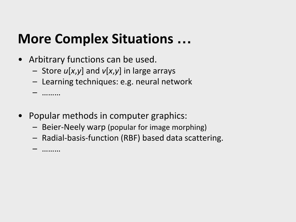
• Arbitrary functions can be used.– Store u[x,y] and v[x,y] in large arrays– Learning techniques: e.g. neural network– ………

• Popular methods in computer graphics:– Beier-Neely warp (popular for image morphing)

– Radial-basis-function (RBF) based data scattering.– ………

More Complex Situations …

• Short for “metamorphosis”.• Early films used cross-dissolving only, but that looks artificial,

non-physical.

• Morph = warp the shape + cross-dissolve the colors.

• If the mappings are defined, cross-dissolving can simply be performed by interpolation.

Morphing

Proposed by Thaddeus Beier, Shawn Neely

Prof. ACM SIGGRAPH’92, pp. 35-42.

Feature-Based Image Metamorphosis

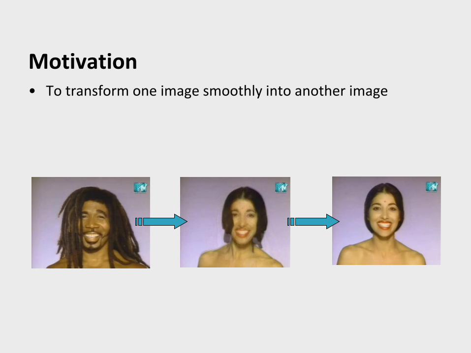
• To transform one image smoothly into another image

Motivation

Overview

Image warping

Image warping

Color Blending

• How to find a controllable mapping function with little manual assistance?

• What’s the problem of mesh-based warping tech.?

• How about the concept of “field”?

Concepts (Beier-Neely warp )

• Features– Points– Lines– Curves– ……

• Fields– Linear– quadratic– ……

How to control the mapping?

Source destination

Using control lines

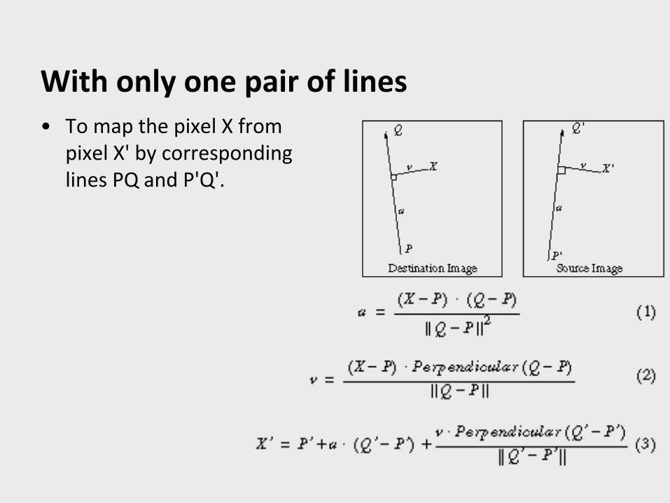
With only one pair of lines• To map the pixel X from

pixel X' by corresponding lines PQ and P'Q'.

With only one pair of lines• Scan every pixels on the destination image and compute the

corresponding pixels on the source image.

An example (only one pair of lines)

• Transforms each pixel coordinate by a rotation, translation ,and/or scale.

• The image is scaled along the direction of lines by the ratio of the length of the line.

• Pure rotation and translation.

• Affine transformations. (uniform scales and shear are not possible to specify.)

The properties of this approach

With multiple pairs of lines• Specifying more complex transformations.

• The displacement Di = Xi’-X.

• A weighted average of these displacements is calculated.

With multiple pairs of lines (cont.)

For each pixel X in the destination

DSUM = (0,0) weightsum = 0

For each line Pi Qicalculate u,v based on Pi Qicalculate X'i based on u,v and Pi'Qi' calculate displacement Di = Xi' - Xi for this line dist = shortest distance from X to Pi Qiweight = (length^p / (a + dist))^b DSUM += Di * weight weightsum += weight

X' = X + DSUM / weightsumdestinationImage(X) = sourceImage(X')

With multiple pairs of lines (cont.)

An example with two line pairs

Morphing between two images

1. Assign the control lines.2. CL(t) = (1-t)CL(0)+t CL(1)3. Generate I0(t), I1(t) according to CL(t)4. I(t) = (1-t)I0(t) + t I1(t)

Source

CL(0)

I(0)

Destination

CL(1)

I(1)

CL(t)

I0(t)

CL(t)

I1(t)

• Interpolating the endpoints of each line.– A rotating line would shrink.

• Interpolating the center position and orientation of each line.– This isn’t very obvious to the user, who might be surprised by how the

lines interpolate.

Two different ways of interpolating

source

destination

intermediate

• It’s much more expressive.

• The animator simply has to describe how lines in a source image are mapped into lines in a destination image.

• The mesh warping is much less intuitive.

Advantages

• This algorithm must compute the effect of every feature line on the movement of that pixel. slow!

• In contrast, mesh warping has only local control .

• Sometimes unexpected interpolations are generated.

• pixel may be far away from all lines.

Disadvantages

Disadvantage (cont.)• The algorithm might make a mistake in computing how that

pixel should move during morphing.

• Need a set of line segments at key frames for each sequence.

Animated sequences

A sequence from Michael Jackson’s MTV “Black or White”

Questions• Is this warping/morphing tech. applicable to all kinds of image

transitions?

2D image morphing

What we want :

• Finding out when image morphing tech. is “correct” (between perspective views)?

• How to extend the image morphing method?

Questions (cont.)

Proposed by S. M. Seitz, C. R. Dyer

Proc. SIGGRAPH’96, pp. 21-30.

View Morphing

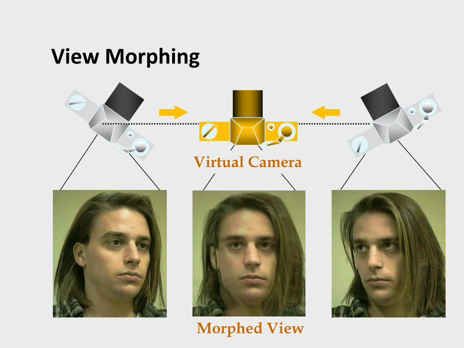
View Morphing

Morphed View

Virtual Camera

View Morphing (cont.)

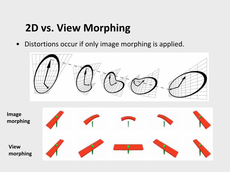
2D vs. View Morphing

• Distortions occur if only image morphing is applied.

Image morphing

View morphing

• 3D modeling with stereo vision techniques.– What’re the advantages and disadvantages?

• Image morphing– Shape-distorting.

• 3D shapes often results in shapes that are mathematically quite different.

– Unless …….

– Is there any special case that image morphing works “correct” for perspective views?

Synthesizing Novel Views

Synthesizing Novel Views (cont.)• Image morphing for perspective views.

– Delicately designing the transition of control lines.• Still requiring an approximate model.

– Parallel views– Linear image interpolation should produce new

perspective views when camera moves parallel to the image plane.

Parallel Views

• Linear image interpolation should produce new perspective views when camera moves parallel to the image plane.

0100

000

000

0

0

0 f

f

M

Projection Matrix M = [ H | -HC ] P^ = MP

Assume

C0 = (0,0,0) C1 = (CX, CY, 0)

0100

00

00

11

11

1 Y

X

Cff

Cff

M

Parallel Views (cont.)

PMZ

PMZ

sPMZ

sspps

s

1

11)1()1( 1010

10)1( sMMsM s

p0 I0 , p1 I1 , P = [X Y Z 1]T

p = (1-s) p0 + s p1 = ?

Cs = (sCX, sCY, 0)

fs = (1-s) f0+s f1

Parallel Views (cont.)• Interpolating images produced from

parallel cameras– Producing the illusion of simultaneously

moving the camera on the line C0C1.

– Moving the optic center and zooming continuously.

• How about non-parallel views?

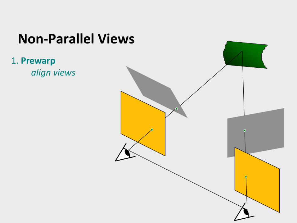
Non-Parallel Views

1. Prewarpalign views

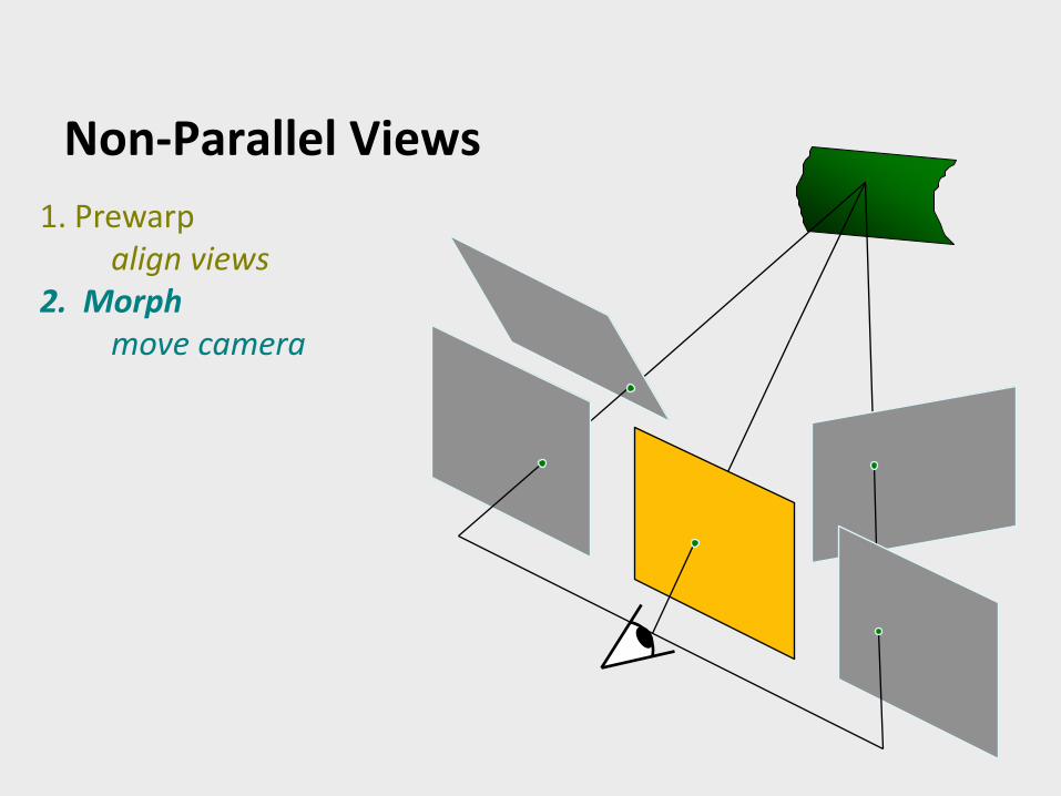
Non-Parallel Views

1. Prewarpalign views

2. Morphmove camera

Non-Parallel Views

1. Prewarpalign views

2. Morph move camera

3. Postwarppoint camera

View Morphing1. Pre-warp:

– Warp the source and destination image to form parallel views.

2. Morphing:– Interpolating the

prewarped images.

3. Post-warp– Warp the interpolated

image to form the Is

1

12

2

3

H0-1

H1-1

Hs

View Morphing (cont.)• For simplicity, the pre-warped images are of f = 1.

0100

010

001

ˆ0

0

0 Y

X

C

C

M

0100

010

001

ˆ1

1

1 Y

X

C

C

M

• Prewarping + morphing + postwarping– Multiple image resampling blurring

• Folds– Occlusion, visibility.

• Holes

Problems

• Prewarping + morphing + postwarping– Multiple image resampling blurring– Solution1: supersampling.– Solution2: aggregate warp.– ……

• Folds– Occlusion, visibility.– Solution1: Comparing Z values (Z-buffer).– Solution2: Disparity– ……

• Holes– Solution1: interpolating (or extrapolating) neighboring pixels.– Solution2: additional images.– ……

Problems (cont.)

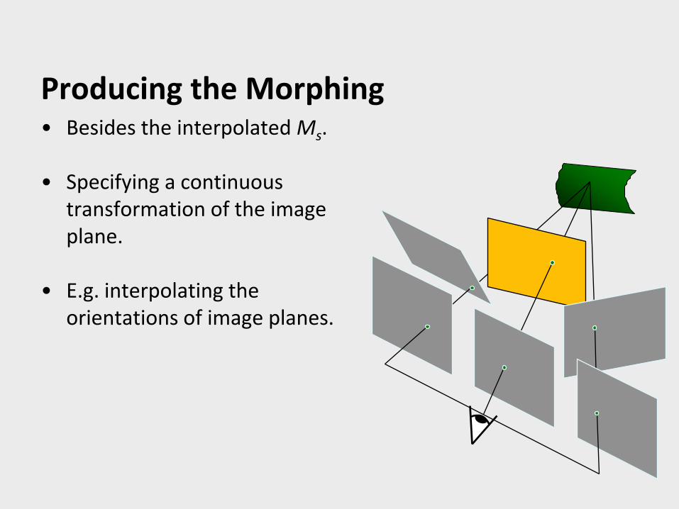
• Besides the interpolated Ms.

• Specifying a continuous transformation of the image plane.

• E.g. interpolating the orientations of image planes.

Producing the Morphing

• Provides– A mobile virtual camera– Better image morphs

• Requires no prior knowledge– No 3D shape information– No dense correspondence– No camera information– No training on other images

• Cons– Limited to interpolation– Problems with occlusions (leads to ghosting)– Prewarp can be unstable (need good F-estimator)

Features of View Morphing

• Visualization– User-controlled virtual camera

• Image postprocessing• Image databases

– Frontal face images for recognition ...

Applications

• Camera calibration– E.g. Camera calibration tool box (for Matlab)– http://www.vision.caltech.edu/bouguetj/calib_doc/

• Through point correspondences– Estimating the fundamental matrix F (or essential matrix E)– We will introduce in the later lecture notes…

How to estimate H?