image enhancement in the frequency domain · image enhancement in the frequency domain gz chapter 4...

Image Enhancement in the frequency domain

GZ Chapter 4

Contents

•  In this lecture we will look at image enhancement in the frequency domain –  The Fourier series & the Fourier transform –  Image Processing in the frequency domain

•  Image smoothing •  Image sharpening

–  Fast Fourier Transform

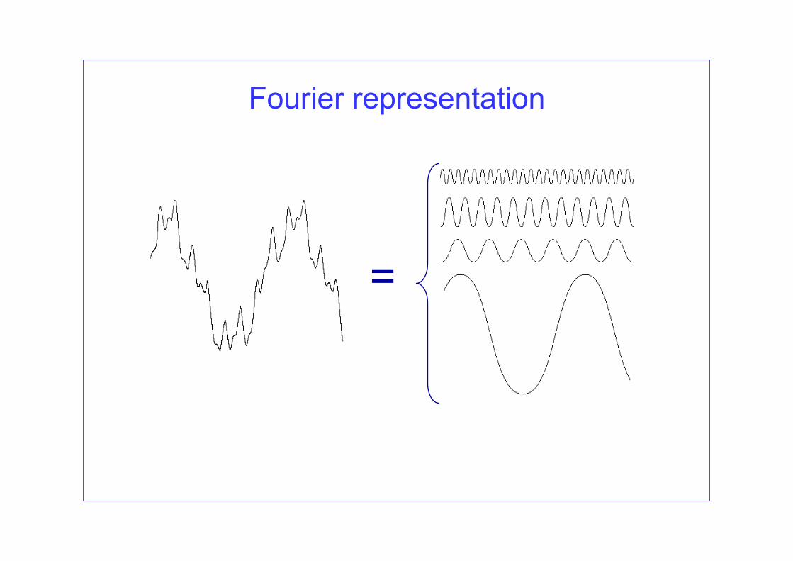
Fourier representation

=

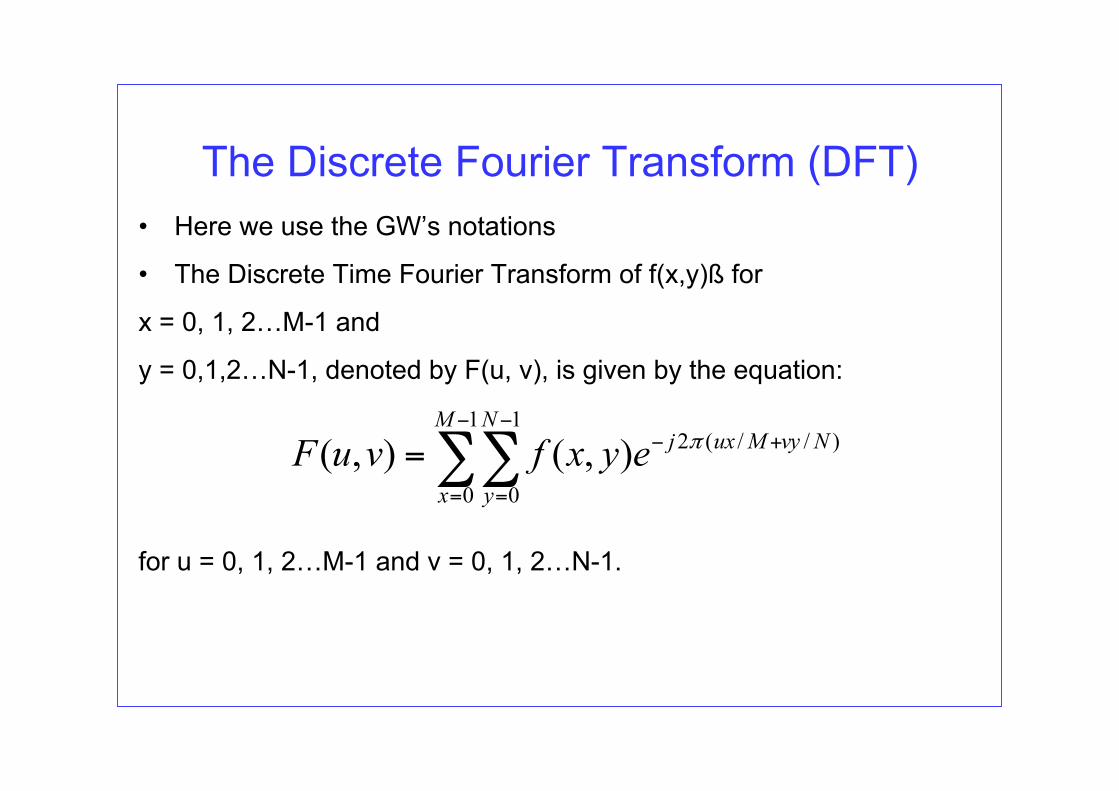
The Discrete Fourier Transform (DFT) •  Here we use the GW’s notations

•  The Discrete Time Fourier Transform of f(x,y)ß for

x = 0, 1, 2…M-1 and

y = 0,1,2…N-1, denoted by F(u, v), is given by the equation:

for u = 0, 1, 2…M-1 and v = 0, 1, 2…N-1.

∑∑−

=

−

=

+−=1

0

1

0

)//(2),(),(M

x

N

y

NvyMuxjeyxfvuF π

The Inverse DFT

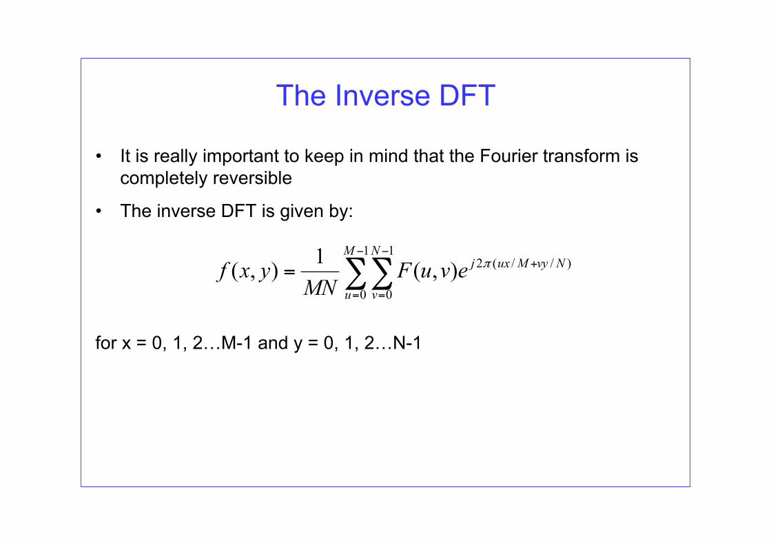
•  It is really important to keep in mind that the Fourier transform is completely reversible

•  The inverse DFT is given by:

for x = 0, 1, 2…M-1 and y = 0, 1, 2…N-1

∑∑−

=

−

=

+=1

0

1

0

)//(2),(1),(M

u

N

v

NvyMuxjevuFMN

yxf π

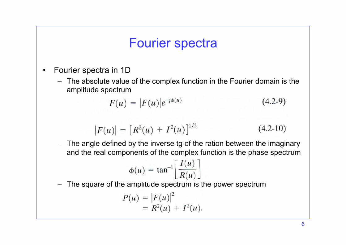
Fourier spectra

•  Fourier spectra in 1D –  The absolute value of the complex function in the Fourier domain is the

amplitude spectrum

–  The angle defined by the inverse tg of the ration between the imaginary and the real components of the complex function is the phase spectrum

–  The square of the amplitude spectrum is the power spectrum

6

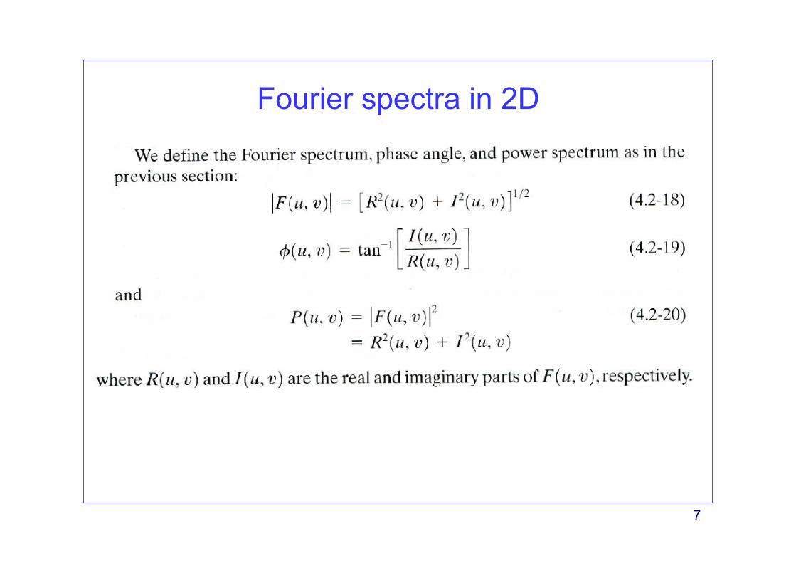
Fourier spectra in 2D

7

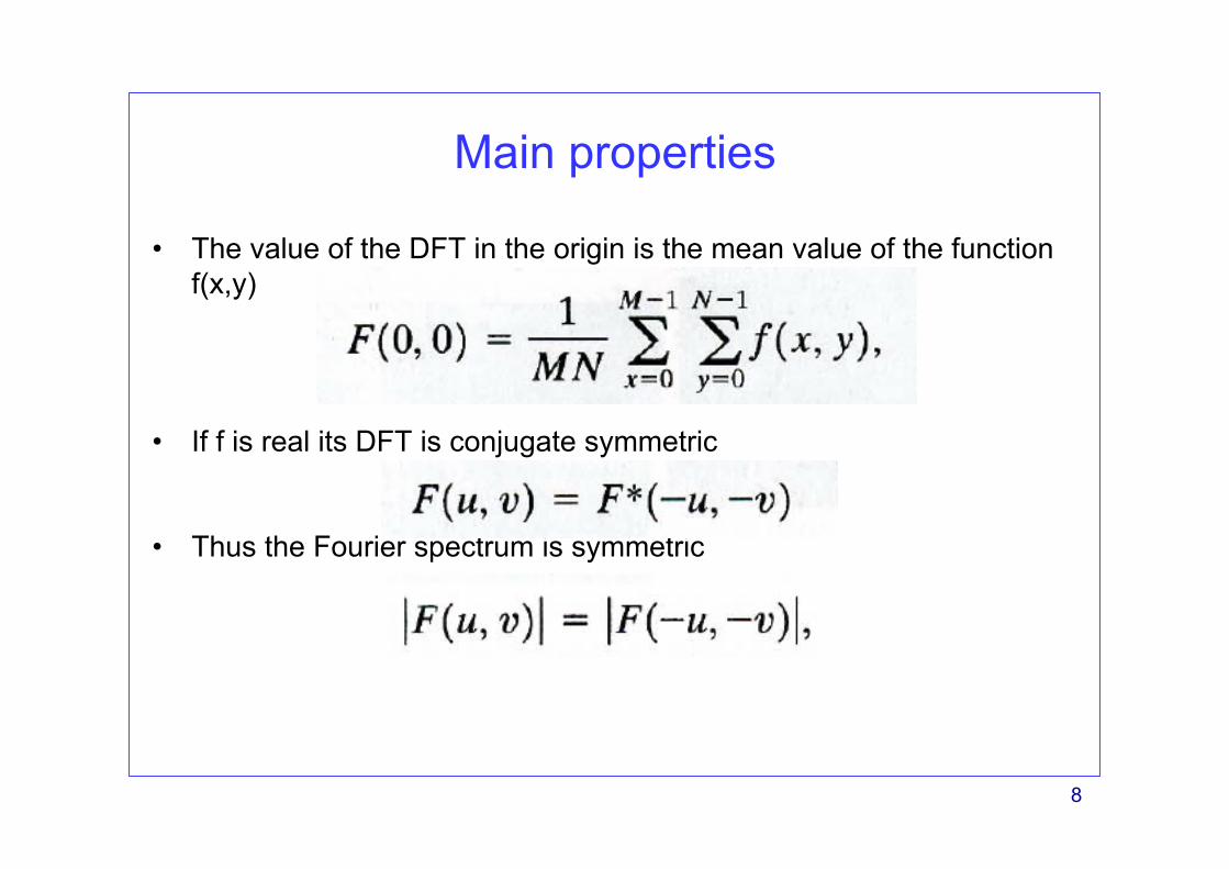
Main properties

•  The value of the DFT in the origin is the mean value of the function f(x,y)

•  If f is real its DFT is conjugate symmetric

•  Thus the Fourier spectrum is symmetric

8

Basics of filtering in the frequency domain

•  To filter an image in the frequency domain: –  Compute F(u,v) the DFT of the image –  Multiply F(u,v) by a filter function H(u,v) –  Compute the inverse DFT of the result

Some Basic Frequency Domain Filters Low Pass Filter (smoothing)

High Pass Filter (edge detection)

Filtering in Fourier domain

•  H(u,v) is the filter transfer function, which is the DFT of the filter impulse response

•  The implementation consists in multiplying point-wise the filter H(u,v) with the function F(u,v)

•  Real filters are called zero phase shift filters because they don’t change the phase of F(u,v)

11

Filtered image

•  The filtered image is obtained by taking the inverse DFT of the resulting image

•  It can happen that the filtered image has spurious imaginary components even though the original image f(x,y) and the filter h(x,y) are real. These are due to numerical errors and are neglected

•  The final result is thus the real part of the filtered image

12

Smoothing: low pass filtering

Edge detection: high-pass filtering Original image

Edge detection: greylevel image

15

Filtered image

16

Hints for filtering

•  Color images are usually converted to graylevel images before filtering. This is due to the fact that the information about the structure of the image (what is in the image) is represented in the luminance component

•  Images are usually stored as “unsigned integers”. Some operations could require the explicit cast to double or float for being implemented

•  The filtered image in general consists of double values, so a cast to unsigned integer could be required before saving it in a file using a predefined format. This could introduce errors due to rounding operations.

17

Frequency Domain Filters

•  The basic model for filtering is:

G(u,v) = H(u,v)F(u,v)

•  where F(u,v) is the Fourier transform of the image being filtered and H(u,v) is the filter transform function

•  Filtered image

•  Smoothing is achieved in the frequency domain by dropping out the high frequency components –  Low pass (LP) filters – only pass the low frequencies, drop the high

ones –  High-pass (HP) filters – olny pass the frequencies above a minimum

value

f x, y( ) =ℑ−1 F u,v( ){ }

LP and HP filtering

19

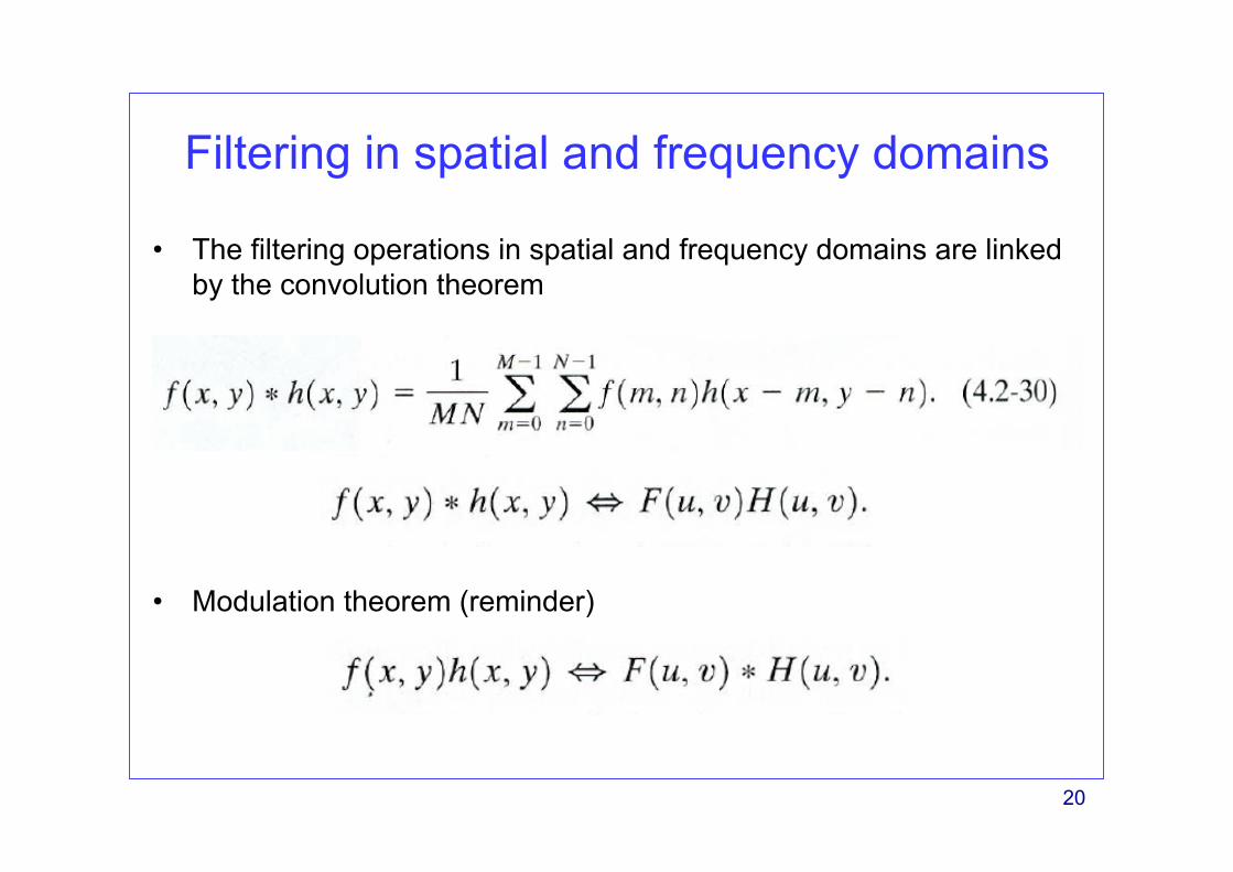
Filtering in spatial and frequency domains

•  The filtering operations in spatial and frequency domains are linked by the convolution theorem

•  Modulation theorem (reminder)

20

Another proof of the convolution theorem

•  Starting from the digital delta function, we will prove that the filtering operation in the signal domain is obtained by the convolution of the signal with the filter impulse response h(x,y)

•  Consider the digital delta function, so an impulse function of strength A located in (x0,y0)

•  Shifting (or sampling) property

21

Getting to the impulse response

•  FT of the delta function located in the origin

•  Now, let’s set f(x,y)=δ(x,y) and calculate the convolution between f and a filter h(x,y)

22

Getting to the impulse response

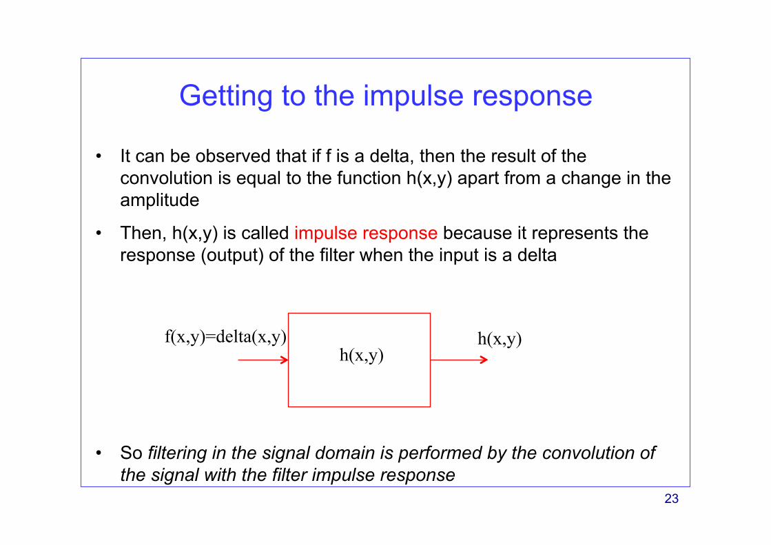
•  It can be observed that if f is a delta, then the result of the convolution is equal to the function h(x,y) apart from a change in the amplitude

•  Then, h(x,y) is called impulse response because it represents the response (output) of the filter when the input is a delta

•  So filtering in the signal domain is performed by the convolution of the signal with the filter impulse response

23

f(x,y)=delta(x,y) h(x,y)

h(x,y)

Filtering: summary

24

Ideal Low Pass Filter

•  Simply cut off all high frequency components that are a specified distance D0 from the origin of the transform

•  changing the distance changes the behaviour of the filter

Ideal Low Pass Filter (cont…)

•  The transfer function for the ideal low pass filter can be given as:

•  where D(u,v) is given as:

⎩⎨⎧

>

≤=

0

0

),( if 0),( if 1

),(DvuDDvuD

vuH

2/122 ])2/()2/[(),( NvMuvuD −+−=


•  Above we show an image, it’s Fourier spectrum and a series of ideal low pass filters of radius 5, 15, 30, 80 and 230 superimposed on top of it


Original image

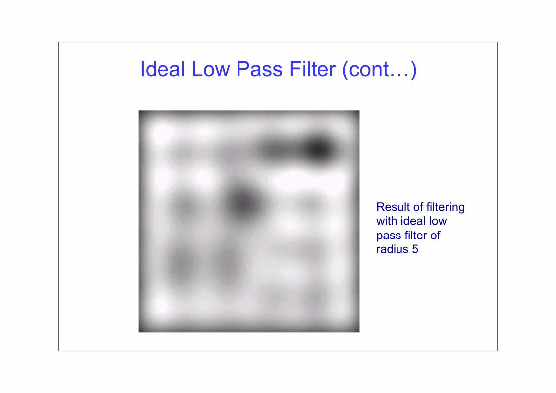
Result of filtering with ideal low pass filter of radius 5



Result of filtering with ideal low

pass filter of radius 80



Butterworth Lowpass Filters

•  The transfer function of a Butterworth lowpass filter of order n with cutoff frequency at distance D0 from the origin is defined as:

nDvuDvuH 2

0 ]/),([11),(

+=

Butterworth Lowpass Filter (cont…)

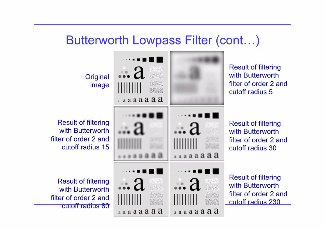
Original image

Result of filtering with Butterworth filter of order 2 and cutoff radius 5



Result of filtering with Butterworth

filter of order 2 and cutoff radius 80




Original image


Gaussian Lowpass Filters

•  The transfer function of a Gaussian lowpass filter is defined as:

20

2 2/),(),( DvuDevuH −=

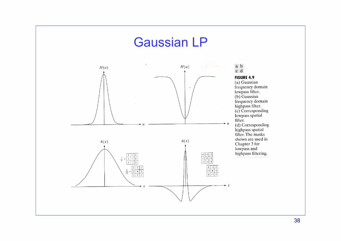
Gaussian LP

38

Gaussian Lowpass Filters (cont…)

Original image

Result of filtering with Gaussian filter with cutoff radius 5



Result of filtering with

Gaussian filter with cutoff radius 85

Result of filtering with Gaussian

filter with cutoff radius 15

Lowpass Filters Compared




Result of filtering with Gaussian

filter with cutoff radius 15

Lowpass Filtering Examples

•  A low pass Gaussian filter is used to connect broken text

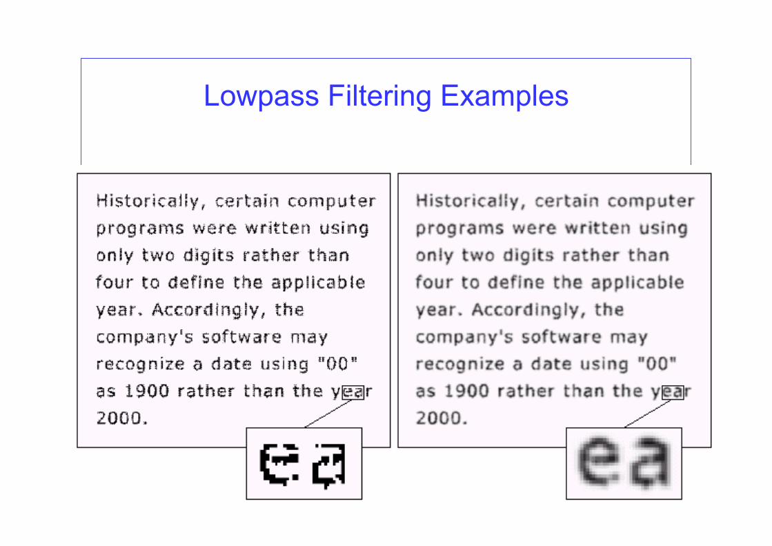
Lowpass Filtering Examples

Lowpass Filtering Examples (cont…)

•  Different lowpass Gaussian filters used to remove blemishes in a photograph

D0=100

D0=80

Lowpass Filtering Examples (cont…)

Original image

Gaussian lowpass filter

Processed image

Spectrum of original image

Sharpening in the Frequency Domain

•  Edges and fine details in images are associated with high frequency components

•  High pass filters – only pass the high frequencies, drop the low ones

•  High pass frequencies are precisely the reverse of low pass filters, so:

•  Hhp(u, v) = 1 – Hlp(u, v)

Ideal High Pass Filters

•  The ideal high pass filter is given as:

•  where D0 is the cut off distance as before

⎩⎨⎧

>

≤=

0

0

),( if 1),( if 0

),(DvuDDvuD

vuH

Ideal High Pass Filters (cont…)

Results of ideal high pass filtering with D0

= 15


= 30


= 80

Butterworth High Pass Filters

•  The Butterworth high pass filter is given as:

•  where n is the order and D0 is the cut off distance as before

nvuDDvuH 2

0 )],(/[11),(

+=

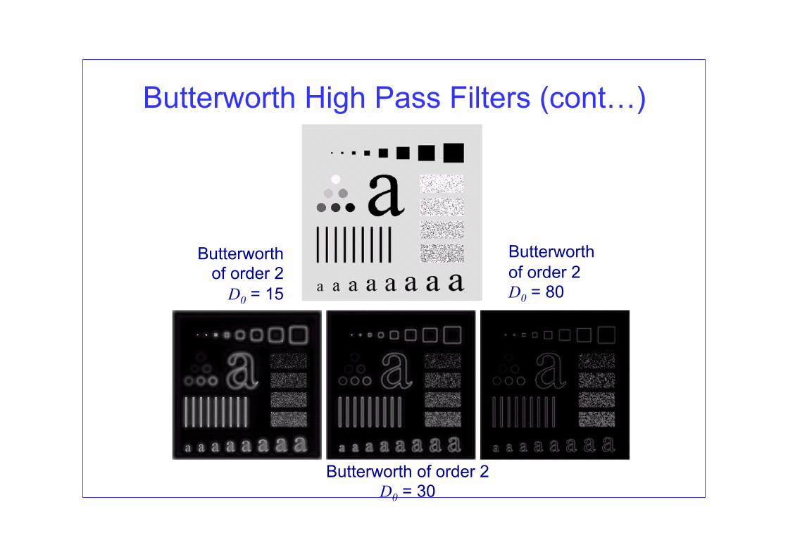
Butterworth High Pass Filters (cont…)

Butterworth of order 2 D0 = 15



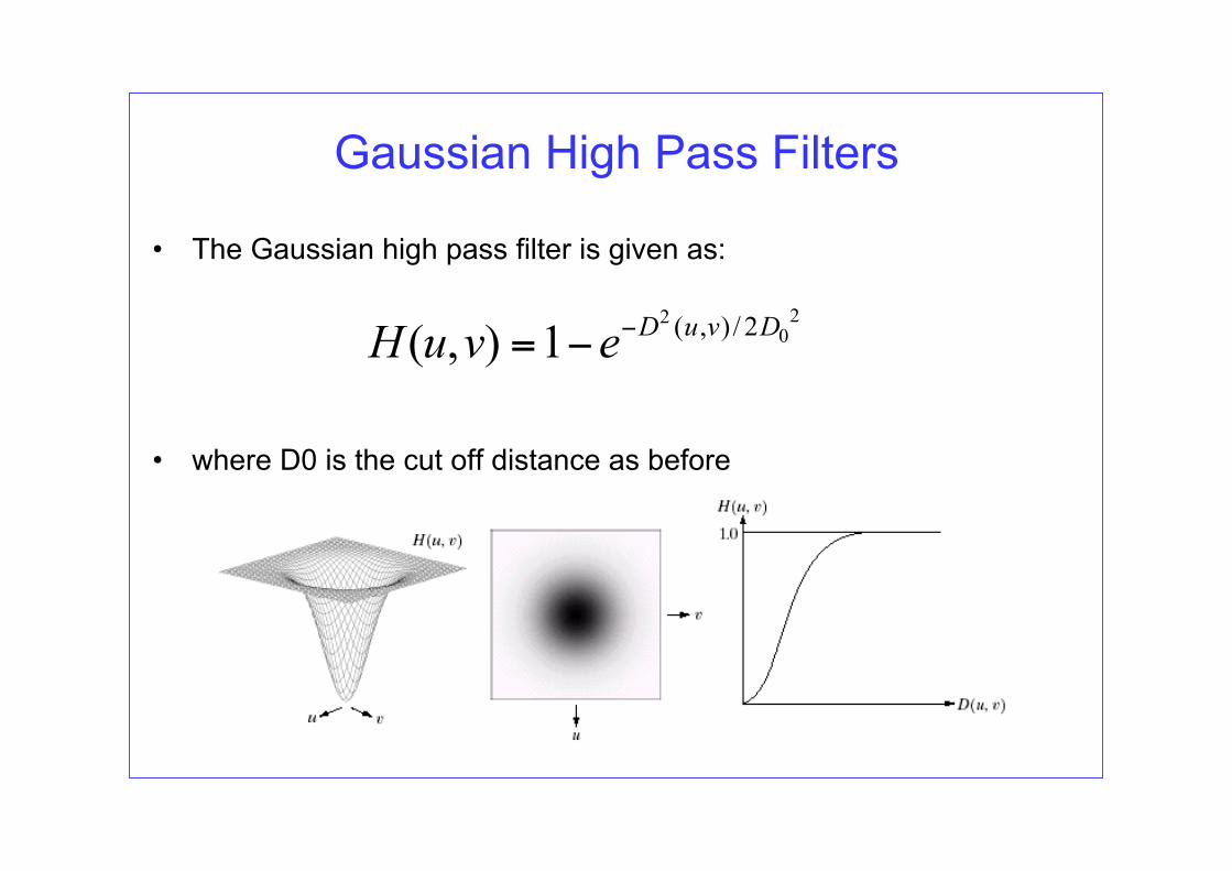
Gaussian High Pass Filters

•  The Gaussian high pass filter is given as:

•  where D0 is the cut off distance as before

20

2 2/),(1),( DvuDevuH −−=

Gaussian High Pass Filters (cont…)

Gaussian high pass D0 = 15



High pass filters comparison

52

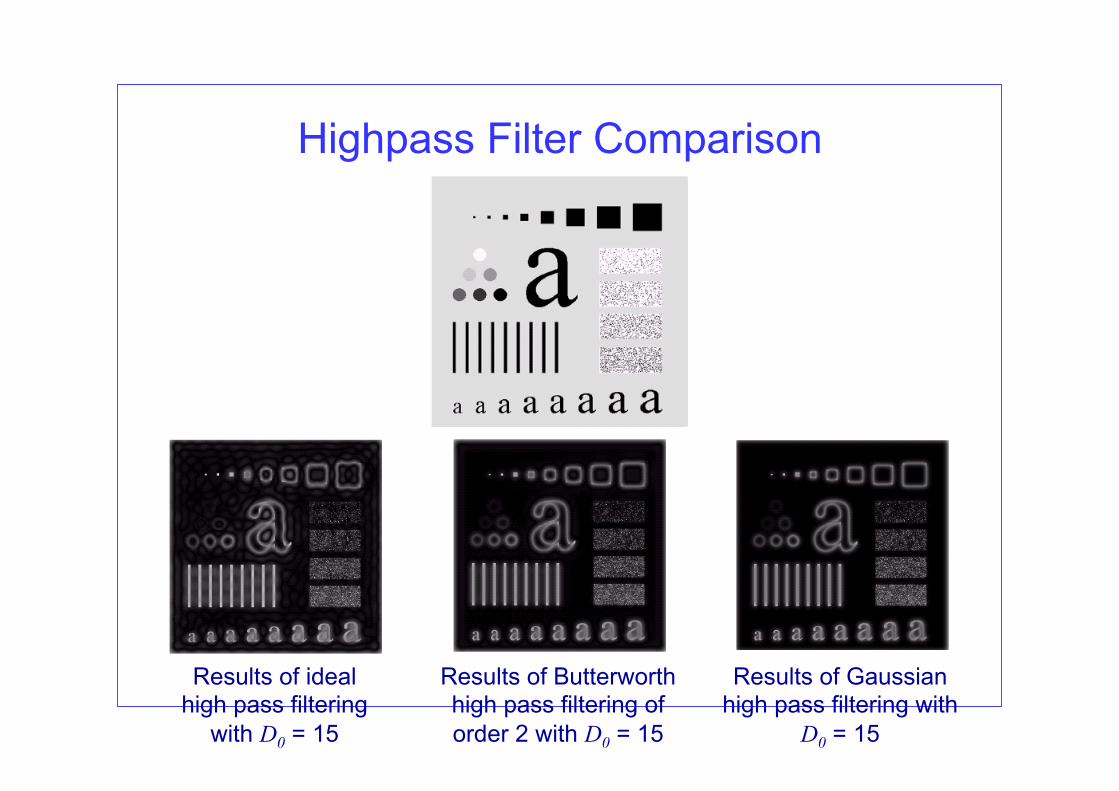
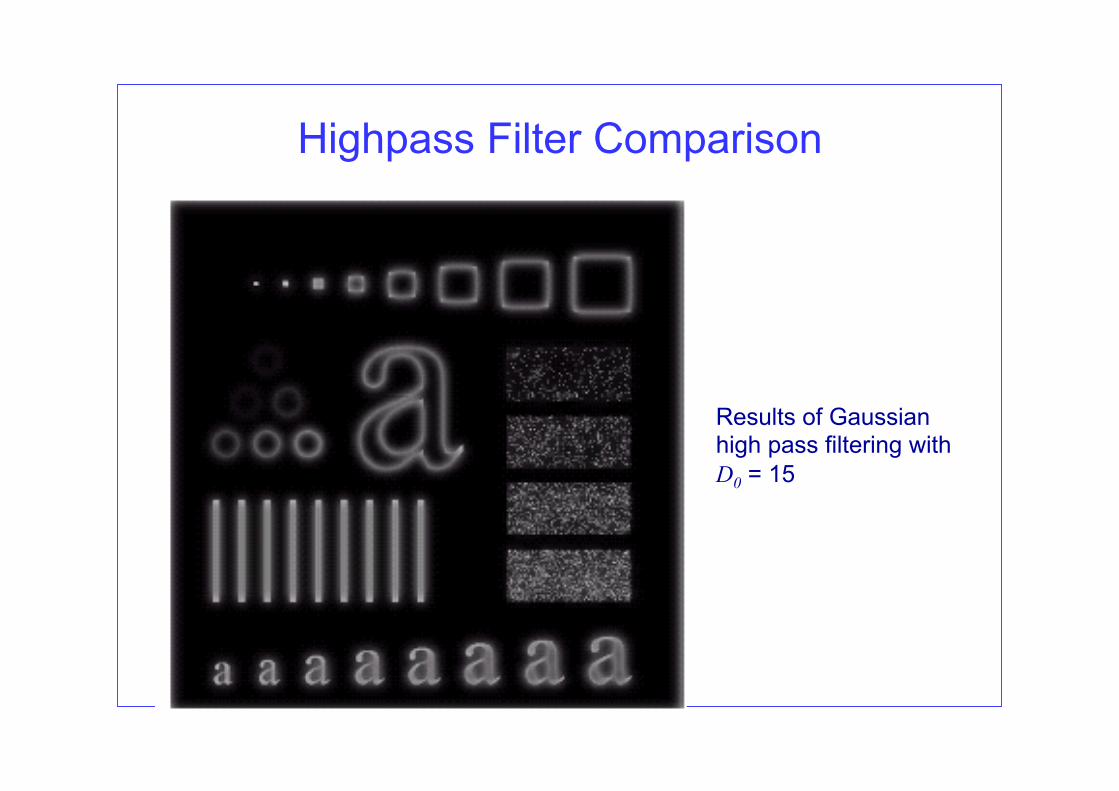
Highpass Filter Comparison

Results of ideal high pass filtering

with D0 = 15

Results of Gaussian high pass filtering with

D0 = 15

Results of Butterworth high pass filtering of order 2 with D0 = 15


Results of ideal high pass filtering with D0 = 15


Results of Butterworth high pass filtering of order 2 with D0 = 15


Results of Gaussian high pass filtering with D0 = 15

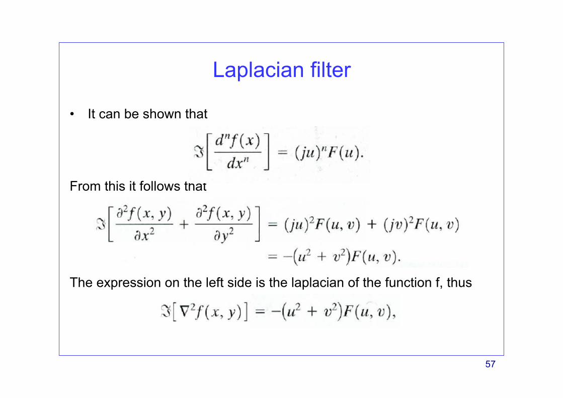
Laplacian filter

•  It can be shown that

From this it follows that

The expression on the left side is the laplacian of the function f, thus

57

Laplacian filter

•  Thus, the Laplacian can be implemented in the Fourier domain by using the filter

58

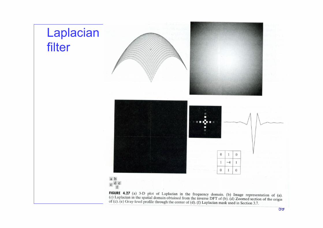
Laplacian filter

59

Laplacian filter

60

High boost filtering

•  A special case of unsharp masking

•  Idea: HP filters cut the zero frequency component, namely the mean value. The resulting image is zero mean and looks very dark

•  High boost filtering “sums” the original image to the result of HPF in order to get an image with sharper (emphasized) edges but with same range of gray values as the original one

•  In formulas –  High pass

–  High boost

61

Signal domain

Frequency domain


fhb x, y( ) = Af x, y( )− flp x, y( )fhb x, y( ) = Af x, y( )− f x, y( )+ f x, y( )− flp x, y( ) == A−1( ) f x, y( )+ fhp x, y( )

62

Reworking the formulas

For A=1 the high-boost corresponds to the HP For A>1 the contribution of the original image becomes larger


•  Note: high pass filtering is also called unsharp filtering

•  In the Fourier domain

63

Hhb u,v( ) = A−1( )H u,v( )+Hhp u,v( )


64

Laplacian

A=2 A=2.7

High boost + histogram equalization

65

Butterworth

High boost equalization

Rest of Chapter 4

•  2D Fourier transform and properties

•  Convolution and correlation

•  Need for padding

•  Fast Fourier Transform (FFT)

66

image enhancement in the frequency domain · image enhancement in the frequency domain gz chapter 4...

Documents