image formation - university of toronto · image formation goal: introduce the elements of camera...

Image Formation

Goal: Introduce the elements of camera models, optics, and image

formation.

Motivation: Camera models, together with radiometry and reflectance

models, allow us to formulate the dependence of image color/intensity

on material reflectance, surface geometry, and lighting.

• Based on these models, we can formulate the inference of scene

properties such as surface shape, reflectance, and scene lighting,

from image data.

• Here we consider the “forward” model. That is, assuming vari-

ous scene and camera properties, what should we observe in an

image?

Readings: Part I (Image Formation and Image Models) of Forsyth

and Ponce.

Matlab Tutorials: colourTutorial.m (in UTVis)

2503: Image Formation c©A.D. Jepson and D.J. Fleet Page: 1

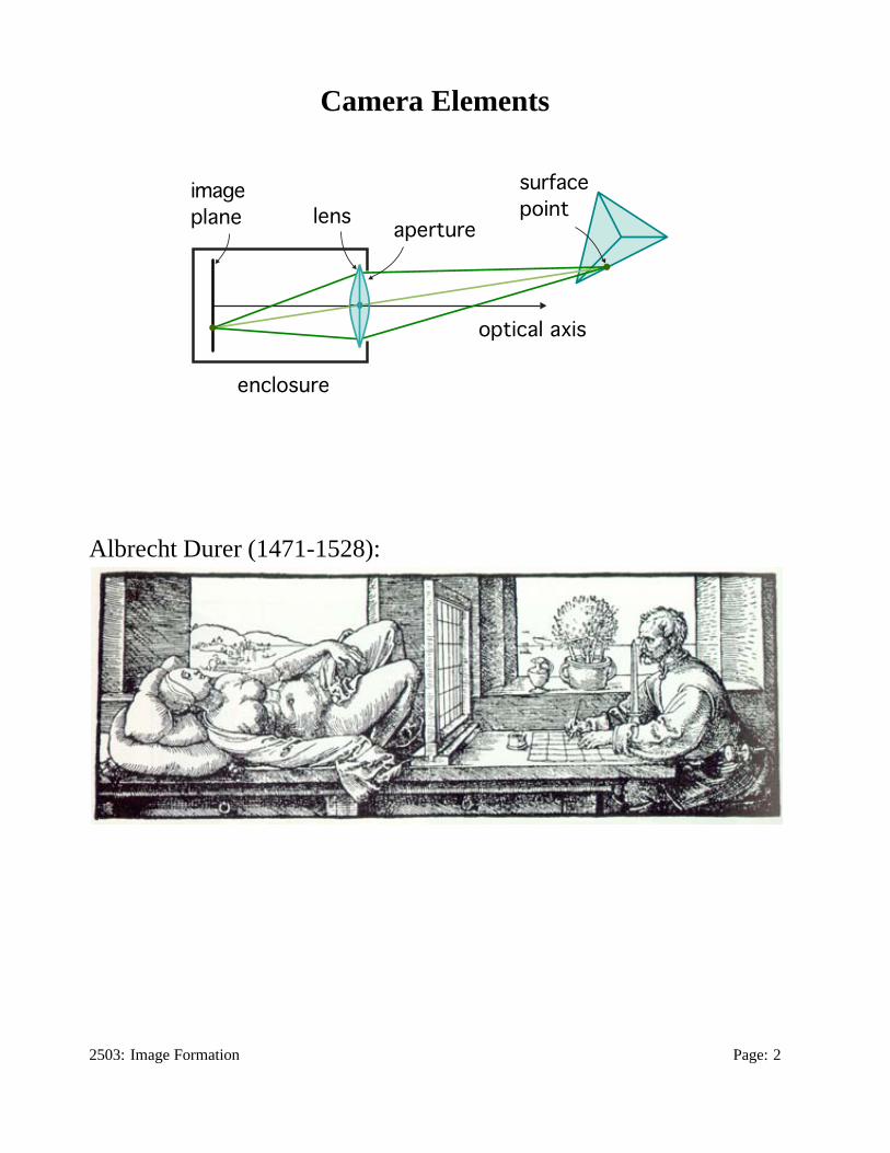
Camera Elements

image

plane lensaperture

surface

point

optical axis

enclosure

Albrecht Durer (1471-1528):

2503: Image Formation Page: 2

Thin Lens

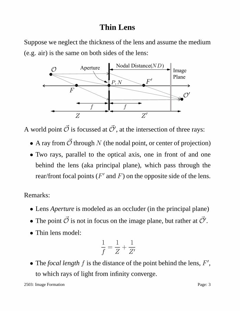
Suppose we neglect the thickness of the lens and assume the medium

(e.g. air) is the same on both sides of the lens:

F′

F

O

O′

f

P,N

f

Z Z′

ApertureImage

Plane

Nodal Distance( )ND

A world point ~O is focussed at~O′, at the intersection of three rays:

• A ray from ~O throughN (the nodal point, or center of projection)

• Two rays, parallel to the optical axis, one in front of and one

behind the lens (aka principal plane), which pass through the

rear/front focal points (F ′ andF ) on the opposite side of the lens.

Remarks:

• LensAperture is modeled as an occluder (in the principal plane)

• The point ~O is not in focus on the image plane, but rather at~O′.

• Thin lens model:

1

f=

1

Z+

1

Z ′

• Thefocal length f is the distance of the point behind the lens,F ′,

to which rays of light from infinity converge.


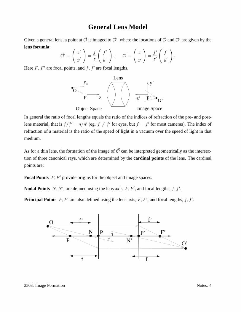
General Lens Model

Given a general lens, a point at~O is imaged to~O′, where the locations of~O and ~O′ are given by the

lens forumla:

~O′ ≡

(

z′

y′

)

=f

z

(

f ′

y

)

, ~O ≡

(

z

y

)

=f ′

z′

(

f

y′

)

.

HereF , F ′ are focal points, andf , f ′ are focal lengths.

Lens

z z’

y’y

O

O’F’

Object Space Image Space

F

In general the ratio of focal lengths equals the ratio of the indices of refraction of the pre- and post-

lens material, that isf/f ′ = n/n′ (eg. f 6= f ′ for eyes, butf = f ′ for most cameras). The index of

refraction of a material is the ratio of the speed of light in avacuum over the speed of light in that

medium.

As for a thin lens, the formation of the image of~O can be interpreted geometrically as the intersec-

tion of three canonical rays, which are determined by thecardinal points of the lens. The cardinal

points are:

Focal Points F, F ′ provide origins for the object and image spaces.

Nodal Points N, N ′, are defined using the lens axis,F, F ′, and focal lengths,f, f ′.

Principal Points P, P ′ are also defined using the lens axis,F, F ′, and focal lengths,f, f ′.

O

O’

f’

ff

f’

F

F’P’N’

PN

2503: Image Formation Notes: 4

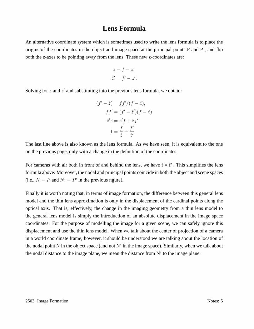
Lens Formula

An alternative coordinate system which is sometimes used towrite the lens formula is to place the

origins of the coordinates in the object and image space at the principal points P and P’, and flip

both the z-axes to be pointing away from the lens. These new z-coordinates are:

z = f − z,

z′ = f ′ − z′.

Solving forz andz′ and substituting into the previous lens formula, we obtain:

(f ′ − z) = ff ′/(f − z),

ff ′ = (f ′ − z′)(f − z)

z′z = z′f + zf ′

1 =f

z+

f ′

z′

The last line above is also known as the lens formula. As we have seen, it is equivalent to the one

on the previous page, only with a change in the definition of the coordinates.

For cameras with air both in front of and behind the lens, we have f = f’. This simplifies the lens

formula above. Moreover, the nodal and principal points coincide in both the object and scene spaces

(i.e.,N = P andN ′ = P ′ in the previous figure).

Finally it is worth noting that, in terms of image formation,the difference between this general lens

model and the thin lens approximation is only in the displacement of the cardinal points along the

optical axis. That is, effectively, the change in the imaging geometry from a thin lens model to

the general lens model is simply the introduction of an absolute displacement in the image space

coordinates. For the purpose of modelling the image for a given scene, we can safely ignore this

displacement and use the thin lens model. When we talk about the center of projection of a camera

in a world coordinate frame, however, it should be understood we are talking about the location of

the nodal point N in the object space (and not N’ in the image space). Similarly, when we talk about

the nodal distance to the image plane, we mean the distance from N’ to the image plane.


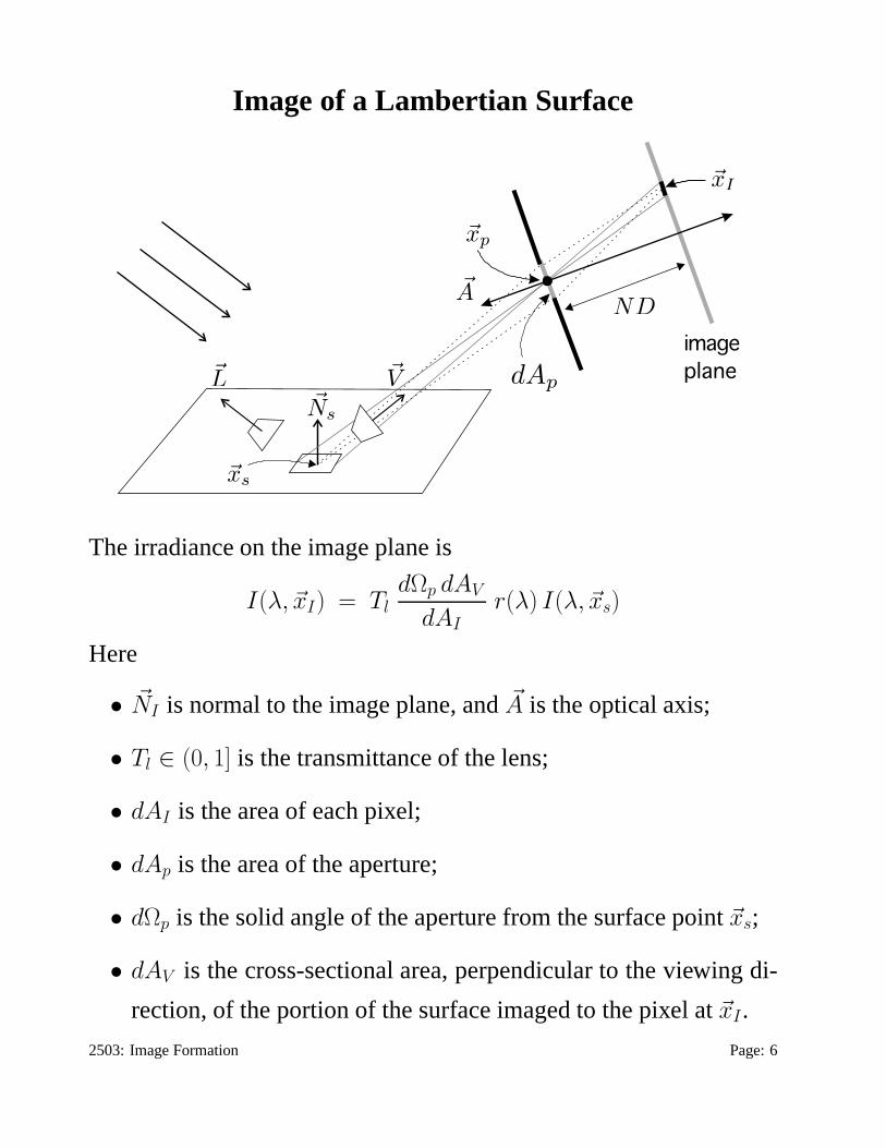
Image of a Lambertian Surface

!L !V

!A

!xI

!xs

!xp

ND

!Ns

image

planedAp

The irradiance on the image plane is

I(λ, ~xI) = TldΩp dAV

dAIr(λ) I(λ, ~xs)

Here

• ~NI is normal to the image plane, and~A is the optical axis;

• Tl ∈ (0, 1] is the transmittance of the lens;

• dAI is the area of each pixel;

• dAp is the area of the aperture;

• dΩp is the solid angle of the aperture from the surface point~xs;

• dAV is the cross-sectional area, perpendicular to the viewing di-

rection, of the portion of the surface imaged to the pixel at~xI .


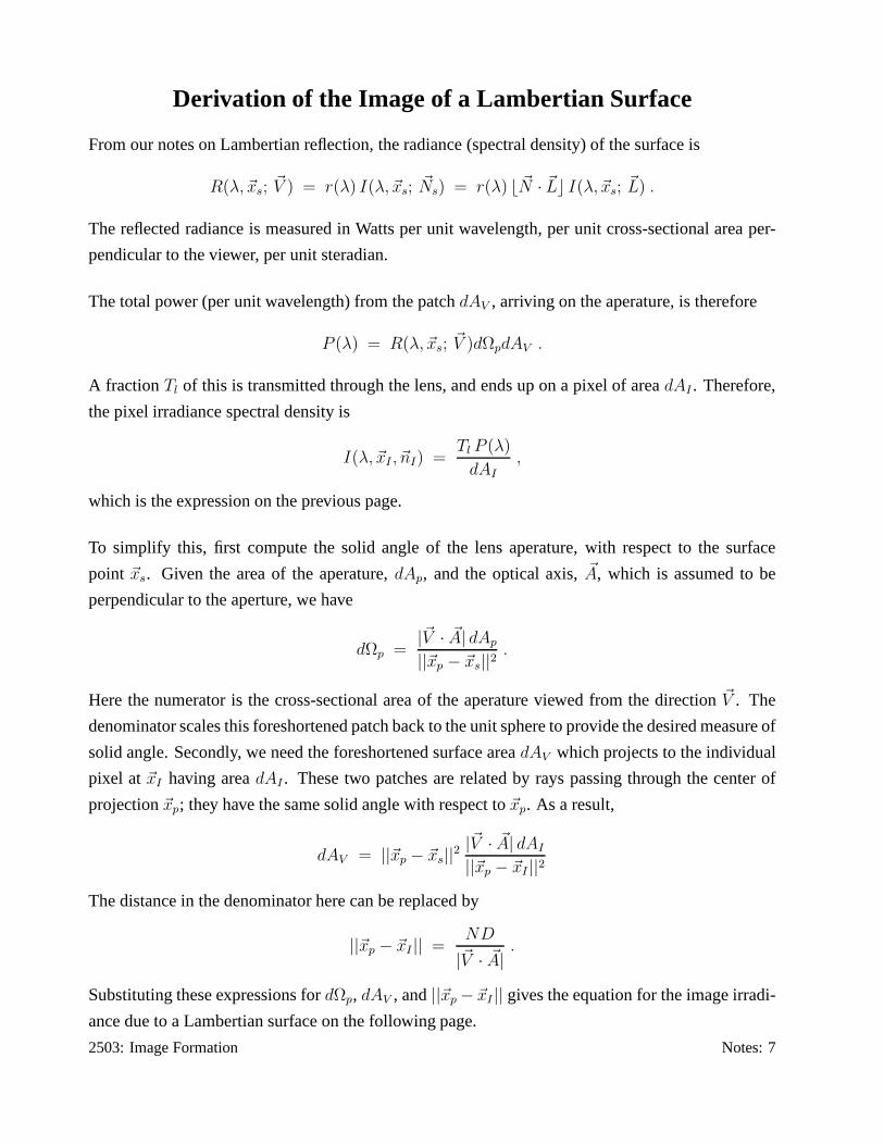
Derivation of the Image of a Lambertian Surface

From our notes on Lambertian reflection, the radiance (spectral density) of the surface is

R(λ, ~xs; ~V ) = r(λ) I(λ, ~xs; ~Ns) = r(λ) ⌊ ~N · ~L⌋ I(λ, ~xs; ~L) .

The reflected radiance is measured in Watts per unit wavelength, per unit cross-sectional area per-

pendicular to the viewer, per unit steradian.

The total power (per unit wavelength) from the patchdAV , arriving on the aperature, is therefore

P (λ) = R(λ, ~xs; ~V )dΩpdAV .

A fraction Tl of this is transmitted through the lens, and ends up on a pixelof areadAI . Therefore,

the pixel irradiance spectral density is

I(λ, ~xI , ~nI) =Tl P (λ)

dAI

,

which is the expression on the previous page.

To simplify this, first compute the solid angle of the lens aperature, with respect to the surface

point ~xs. Given the area of the aperature,dAp, and the optical axis,~A, which is assumed to be

perpendicular to the aperture, we have

dΩp =|~V · ~A| dAp

||~xp − ~xs||2.

Here the numerator is the cross-sectional area of the aperature viewed from the direction~V . The

denominator scales this foreshortened patch back to the unit sphere to provide the desired measure of

solid angle. Secondly, we need the foreshortened surface areadAV which projects to the individual

pixel at~xI having areadAI . These two patches are related by rays passing through the center of

projection~xp; they have the same solid angle with respect to~xp. As a result,

dAV = ||~xp − ~xs||2|~V · ~A| dAI

||~xp − ~xI ||2

The distance in the denominator here can be replaced by

||~xp − ~xI || =ND

|~V · ~A|.

Substituting these expressions fordΩp, dAV , and||~xp − ~xI || gives the equation for the image irradi-

ance due to a Lambertian surface on the following page.


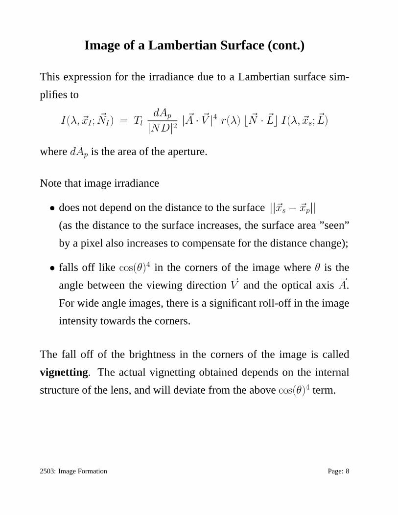
Image of a Lambertian Surface (cont.)

This expression for the irradiance due to a Lambertian surface sim-

plifies to

I(λ, ~xI ; ~NI) = TldAp

|ND|2| ~A · ~V |4 r(λ) ⌊ ~N · ~L⌋ I(λ, ~xs; ~L)

wheredAp is the area of the aperture.

Note that image irradiance

• does not depend on the distance to the surface||~xs − ~xp||

(as the distance to the surface increases, the surface area ”seen”

by a pixel also increases to compensate for the distance change);

• falls off like cos(θ)4 in the corners of the image whereθ is the

angle between the viewing direction~V and the optical axis~A.

For wide angle images, there is a significant roll-off in the image

intensity towards the corners.

The fall off of the brightness in the corners of the image is called

vignetting. The actual vignetting obtained depends on the internal

structure of the lens, and will deviate from the abovecos(θ)4 term.


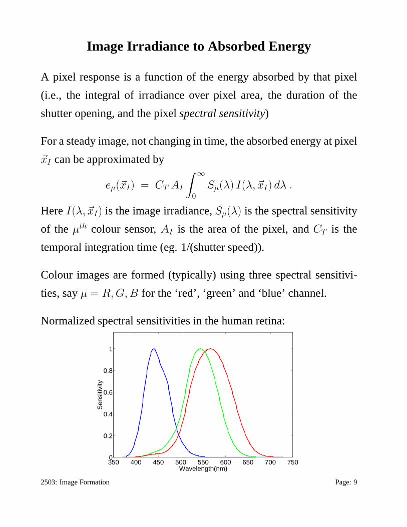
Image Irradiance to Absorbed Energy

A pixel response is a function of the energy absorbed by that pixel

(i.e., the integral of irradiance over pixel area, the duration of the

shutter opening, and the pixelspectral sensitivity)

For a steady image, not changing in time, the absorbed energyat pixel

~xI can be approximated by

eµ(~xI) = CT AI

∫ ∞

0

Sµ(λ) I(λ, ~xI) dλ .

HereI(λ, ~xI) is the image irradiance,Sµ(λ) is the spectral sensitivity

of the µth colour sensor,AI is the area of the pixel, andCT is the

temporal integration time (eg. 1/(shutter speed)).

Colour images are formed (typically) using three spectral sensitivi-

ties, sayµ = R, G, B for the ‘red’, ‘green’ and ‘blue’ channel.

Normalized spectral sensitivities in the human retina:

350 400 450 500 550 600 650 700 7500

0.2

0.4

0.6

0.8

1

Wavelength(nm)

Sen

sitiv

ity


Absorbed Energy to Pixel Response

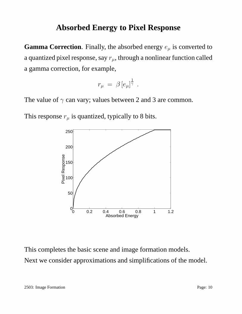
Gamma Correction. Finally, the absorbed energyeµ is converted to

a quantized pixel response, sayrµ, through a nonlinear function called

a gamma correction, for example,

rµ = β [eµ]1

γ .

The value ofγ can vary; values between 2 and 3 are common.

This responserµ is quantized, typically to 8 bits.

0 0.2 0.4 0.6 0.8 1 1.20

50

100

150

200

250

Absorbed Energy

Pix

el R

espo

nse

This completes the basic scene and image formation models.

Next we consider approximations and simplifications of the model.


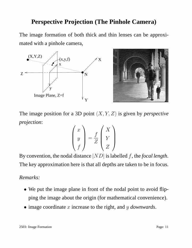
Perspective Projection (The Pinhole Camera)

The image formation of both thick and thin lenses can be approxi-

mated with a pinhole camera,

X

Z

Y

(X,Y,Z)(x,y,f)

N

y

x

Image Plane, Z=f

The image position for a 3D point(X, Y, Z) is given byperspective

projection:

x

y

f

=f

Z

X

Y

Z

By convention, the nodal distance|ND| is labelledf , thefocal length.

The key approximation here is that all depths are taken to be in focus.

Remarks:

• We put the image plane in front of the nodal point to avoid flip-

ping the image about the origin (for mathematical convenience).

• image coordinatex increase to the right, andy downwards.


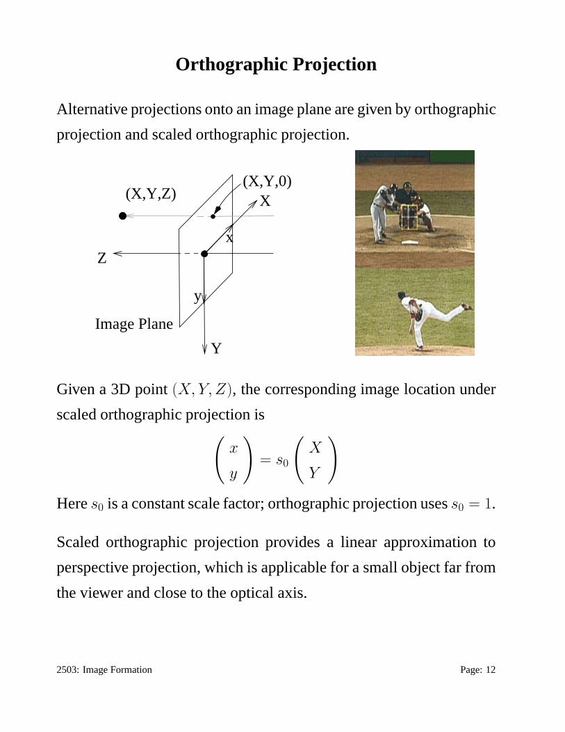
Orthographic Projection

Alternative projections onto an image plane are given by orthographic

projection and scaled orthographic projection.

(X,Y,Z)

Zx

Image Plane

X

y

Y

(X,Y,0)

Given a 3D point(X, Y, Z), the corresponding image location under

scaled orthographic projection is(

x

y

)

= s0

(

X

Y

)

Heres0 is a constant scale factor; orthographic projection usess0 = 1.

Scaled orthographic projection provides a linear approximation to

perspective projection, which is applicable for a small object far from

the viewer and close to the optical axis.


Coordinate Frames

Consider the three coordinate frames:

• a world coordinate frame~Xw,

• a camera coordinate frame,~Xc,

• an image coordinate frame,~p.

The world and camera frames provide standard 3D orthogonal co-

ordinates. The image coordinates are written as a 3-vector,~p =

(p1, p2, 1)T , with p1 andp2 the pixel coordinates of the image point.

Camera Coordinate Frame. The origin of the camera coordinates

is at the nodal point of the camera (say at~dw in world coords). Thez-

axis is taken to be the optical axis of the camera (with pointsin front

of the camera having a positivez value).

Image formation requires that we specify two mappings, i.e., from

world to camera coordinates, and fromcamera to image coordinates.


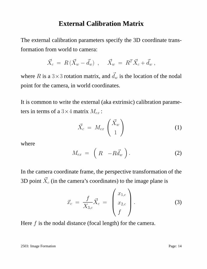
External Calibration Matrix

The external calibration parameters specify the 3D coordinate trans-

formation from world to camera:

~Xc = R ( ~Xw − ~dw) , ~Xw = RT ~Xc + ~dw ,

whereR is a3×3 rotation matrix, and~dw is the location of the nodal

point for the camera, in world coordinates.

It is common to write the external (aka extrinsic) calibration parame-

ters in terms of a3×4 matrixMex :

~Xc = Mex

(

~Xw

1

)

(1)

where

Mex =(

R −R~dw

)

. (2)

In the camera coordinate frame, the perspective transformation of the

3D point ~Xc (in the camera’s coordinates) to the image plane is

~xc =f

X3,c

~Xc =

x1,c

x2,c

f

. (3)

Heref is the nodal distance (focal length) for the camera.


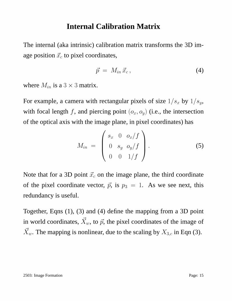
Internal Calibration Matrix

The internal (aka intrinsic) calibration matrix transforms the 3D im-

age position~xc to pixel coordinates,

~p = Min ~xc , (4)

whereMin is a3 × 3 matrix.

For example, a camera with rectangular pixels of size1/sx by 1/sy,

with focal lengthf , and piercing point(ox, oy) (i.e., the intersection

of the optical axis with the image plane, in pixel coordinates) has

Min =

sx 0 ox/f

0 sy oy/f

0 0 1/f

. (5)

Note that for a 3D point~xc on the image plane, the third coordinate

of the pixel coordinate vector,~p, is p3 = 1. As we see next, this

redundancy is useful.

Together, Eqns (1), (3) and (4) define the mapping from a 3D point

in world coordinates,~Xw, to ~p, the pixel coordinates of the image of~Xw. The mapping is nonlinear, due to the scaling byX3,c in Eqn (3).


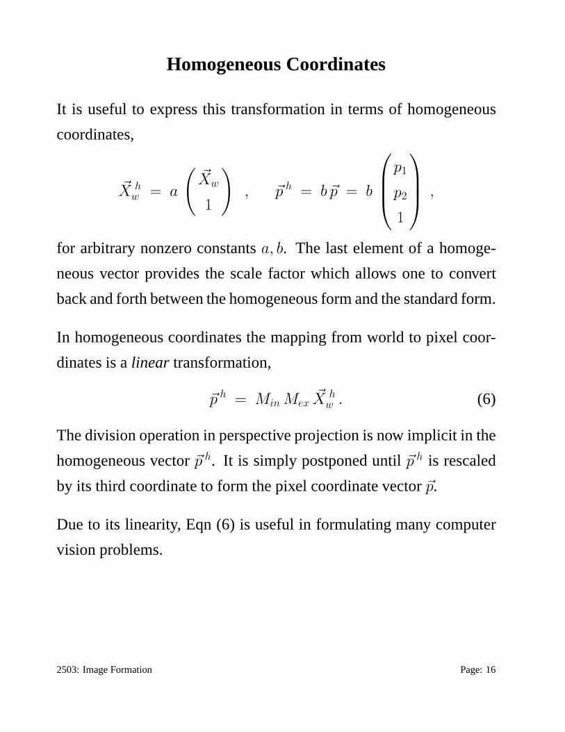
Homogeneous Coordinates

It is useful to express this transformation in terms of homogeneous

coordinates,

~X hw = a

(

~Xw

1

)

, ~p h = b ~p = b

p1

p2

1

,

for arbitrary nonzero constantsa, b. The last element of a homoge-

neous vector provides the scale factor which allows one to convert

back and forth between the homogeneous form and the standardform.

In homogeneous coordinates the mapping from world to pixel coor-

dinates is alinear transformation,

~p h = Min Mex~X h

w . (6)

The division operation in perspective projection is now implicit in the

homogeneous vector~p h. It is simply postponed until~p h is rescaled

by its third coordinate to form the pixel coordinate vector~p.

Due to its linearity, Eqn (6) is useful in formulating many computer

vision problems.


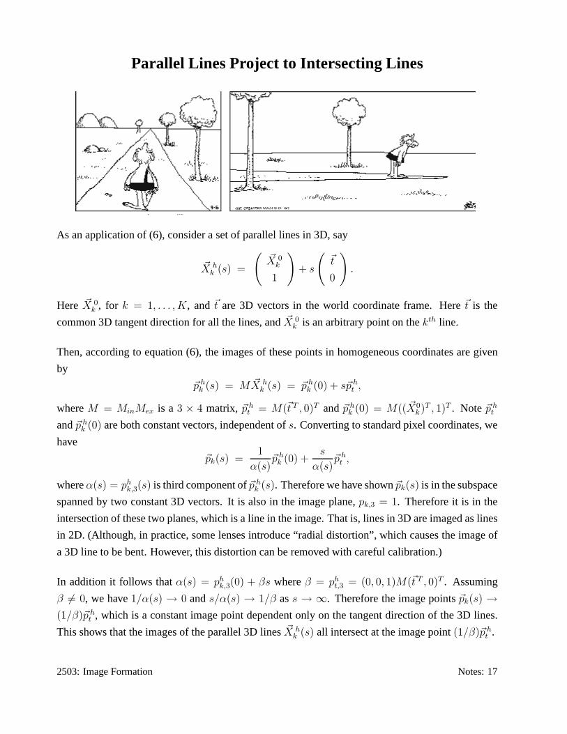
Parallel Lines Project to Intersecting Lines

As an application of (6), consider a set of parallel lines in 3D, say

~X hk (s) =

(

~X 0

k

1

)

+ s

(

~t

0

)

.

Here ~X 0

k , for k = 1, . . . , K, and~t are 3D vectors in the world coordinate frame. Here~t is the

common 3D tangent direction for all the lines, and~X 0

k is an arbitrary point on thekth line.

Then, according to equation (6), the images of these points in homogeneous coordinates are given

by

~p hk (s) = M ~X h

k (s) = ~p hk (0) + s~p h

t ,

whereM = MinMex is a 3 × 4 matrix, ~p ht = M(~t T , 0)T and~p h

k (0) = M(( ~X0

k)T , 1)T . Note~p ht

and~p hk (0) are both constant vectors, independent ofs. Converting to standard pixel coordinates, we

have

~pk(s) =1

α(s)~p h

k (0) +s

α(s)~p h

t ,

whereα(s) = phk,3(s) is third component of~p h

k (s). Therefore we have shown~pk(s) is in the subspace

spanned by two constant 3D vectors. It is also in the image plane,pk,3 = 1. Therefore it is in the

intersection of these two planes, which is a line in the image. That is, lines in 3D are imaged as lines

in 2D. (Although, in practice, some lenses introduce “radial distortion”, which causes the image of

a 3D line to be bent. However, this distortion can be removed with careful calibration.)

In addition it follows thatα(s) = phk,3(0) + βs whereβ = ph

t,3 = (0, 0, 1)M(~t T , 0)T . Assuming

β 6= 0, we have1/α(s) → 0 ands/α(s) → 1/β ass → ∞. Therefore the image points~pk(s) →

(1/β)~p ht , which is a constant image point dependent only on the tangent direction of the 3D lines.

This shows that the images of the parallel 3D lines~X hk (s) all intersect at the image point(1/β)~p h

t .


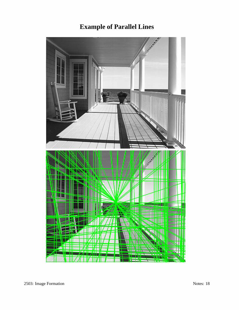
Example of Parallel Lines


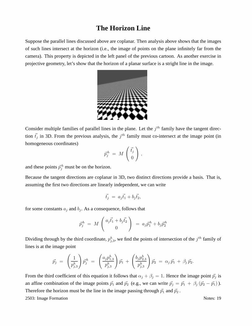
The Horizon Line

Suppose the parallel lines discussed above are coplanar. Then analysis above shows that the images

of such lines intersect at the horizon (i.e., the image of points on the plane infinitely far from the

camera). This property is depicted in the left panel of the previous cartoon. As another exercise in

projective geometry, let’s show that the horizon of a planarsurface is a stright line in the image.

Consider multiple families of parallel lines in the plane. Let thejth family have the tangent direc-

tion ~tj in 3D. From the previous analysis, thejth family must co-intersect at the image point (in

homogeneous coordinates)

~p hj = M

(

~tj

0

)

,

and these points~p hj must be on the horizon.

Because the tangent directions are coplanar in 3D, two distinct directions provide a basis. That is,

assuming the first two directions are linearly independent,we can write

~tj = aj~t1 + bj

~t2,

for some constantsaj andbj . As a consequence, follows that

~p hj = M

(

aj~t1 + bj

~t2

0

)

= aj~ph1

+ bj~ph2

Dividing through by the third coordinate,phj,3, we find the points of intersection of thejth family of

lines is at the image point

~pj =

(

1

phj,3

)

~p hj =

(

ajph1,3

phj,3

)

~p1 +

(

bjph2,3

phj,3

)

~p2 = αj ~p1 + βj ~p2.

From the third coefficient of this equation it follows thatαj + βj = 1. Hence the image point~pj is

an affine combination of the image points~p1 and~p2 (e.g., we can write~pj = ~p1 + βj (~p2 − ~p1) ).

Therefore the horizon must be the line in the image passing through~p1 and~p2 .


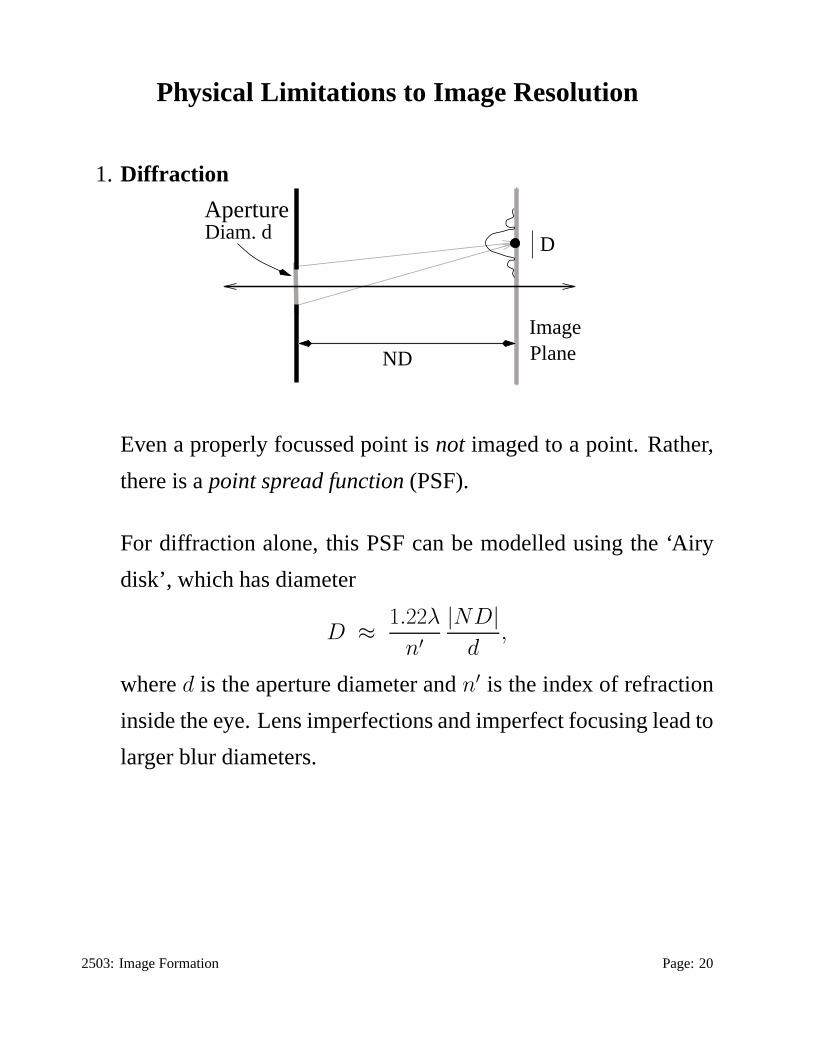
Physical Limitations to Image Resolution

1. Diffraction

Image

ND Plane

DDiam. dAperture

Even a properly focussed point isnot imaged to a point. Rather,

there is apoint spread function (PSF).

For diffraction alone, this PSF can be modelled using the ‘Airy

disk’, which has diameter

D ≈1.22λ

n′

|ND|

d,

whered is the aperture diameter andn′ is the index of refraction

inside the eye. Lens imperfections and imperfect focusing lead to

larger blur diameters.


Diffraction Limit (cont.)

For human eyes (see Wyszecki & Stiles, Color Science, 1982):

• the index of refraction within the eye isn′ = 1.33;

• the nodal distance is|ND| ≈ 16.7mm (accommodated at∞);

• the pupil diameter isd ≈ 2mm (adapted to bright conditions);

• a typical wavelength isλ ≈ 500nm.

Therefore the diameter of the Airy disk is

D ≈ 4µ = 4 × 10−6m

This compares closely to the diameter of a foveal cone (i.e. the small-

est pixel), which is between1µ and4µ. So, human vision operates at

the diffraction limit.

By the way, a2µ pixel spacing in the human eye corresponds to hav-

ing a 300 × 300 pixel resolution of the image of your thumbnail at

arm’s length. Compare this to the typical sizes of images used by

machine vision systems, usually about1000 × 1000.


2. Photon Noise

The average photon flux (spectral density) at the image (in units

of photons per sec, per unit wavelength, per image area) is

I(λ, ~xI ; ~NI)λ

hc

Hereh is Planck’s constant andc is the speed of light.

The photon arrivals can be modelled with Poisson statistics, so

the variance is equal to the mean photon catch.

Even in bright conditions, foveal cones have a significant photon

noise component (a std. dev.≈ 10% of the signal, for unshaded

scenes).

3. Defocus

An improperly focussed lens causes the PSF to broaden. Geo-

metrical optics can be used to get a rough estimate of the size.

4. Motion Blur

Given temporal averaging, the image of a moving point forms a

streak in the image, causing further blur.

Conclude: There is a limit to how small standard cameras and eyes

can be made (but note multi-faceted insect eyes). Human vision op-

erates close to the physical limits of resolution (ditto forinsects).


image formation - university of toronto · image formation goal: introduce the elements of camera...

Documents