image harmonization - about

Image Harmonization

Processing math: 100%

Overall Pipeline

2/35Processing math: 100%

Motivation

Multi-site imaging studies are becoming increasingly common.

Combining imaging data across sites introduces non-biological sources of variationthat arise from the use of different scanner hardware and acquisition protocols.

Scanner effects or site effects are similar to batch effects in the genomics literature

·

·

E.g., field strength, manufacturer, subject positioning-

·

Known to affect measurement of regional volumes, cortical thickness, voxel-basedmorphometry, …

More generally, structural, functional, diffusion tensor, and other types of imagesand features extracted from them may exhibit scanner effects

-

-


Motivation

Need to eliminate or account for scanner effects in downstream statistical analyses

Several methods for estimating and removing unwanted sources of variation due tosite/scanner have been adapted to neuroimaging data.

In this tutorial we will use ComBat (Johnson, Li, and Rabinovic 2007; Fortin et al. 2018)to harmonize cortical thicknesses from the ADNI data.

·

Most critical if sites or scanners are imbalanced with respect to other variablessuch as age, sex, race, clinical status

Simply including scanner as a confounding variable may not work well (Rao etal. 2017)

-

-

·

·

ComBat has been shown to effectively reduce scanner-to-scanner variability whilepreserving biological associations.

-


ADNI Cortical Thickness Data

The Alzheimer’s Disease Neuroimaging Initiative (ADNI) is a multi-million dollar studyfunded by public and private sources.

The goals of the ADNI are to better understand progression from normal aging to mildcognitive impairment (MCI) and early Alzheimer’s disease (AD) and determine effectivebiomarkers for disease diagnosis, monitoring, and treatment development.

We estimated cortical thicknesses from a subset of initial subject visits (N=187)

Our subset consists of images aquired from scanners at 17 different sites

·

National Institute on Aging, the National Institute of Biomedical Imaging andBioengineering, the Food and Drug Administration, private pharmaceuticalcompanies, and non-profit organizations.

-

·

·

Mix of male/female aged 56-91

Mix of healthy controls (46), MCI (93), and AD (48) diagnoses at baseline

-

-

·

Mix of field strength, manufacturer, and model-


ADNI Data Access

http://adni.loni.usc.edu/data-samples/access-data/


http://adni.loni.usc.edu/data-samples/access-data/

Image taken from http://www.martinos.org/neurorecovery/technology.htm

Cortical Thickness

There are several different ways tomeasure cortical thickness

General idea is to measure perpendicularfrom the white/gray matter boundary tothe pial surface

Cortical thickness is an importantimaging-based biomarker for numerouspsychological and neurodegenerativediseases: Alzheimer’s and otherdementias, Schizophrenia, MS, addiction,…

·

·

·


http://www.martinos.org/neurorecovery/technology.htm

ANTS Cortical Thickness Pipeline (antsCorticalThickness.sh)

DiReCT: Diffeomorphic Registration based CT measurement (Das et al. 2009)

With results from Atropos, can use cort_thickness in extrantsr package

·

·


Cortical Thickness Regions

Multi-atlas label fusion applied using 20 OASIS template T1s manually labeled with theDesikan-Killiany-Tourville (DKT) cortical labeling protocol (www.mindboggle.info).

·

label roi 1 X1002 “left caudal anterior cingulate” 2 X1003 “left caudal middle frontal” 3 X1005 “left cuneus” 4 X1008 “left inferior parietal” 5 X1017 “left paracentral” 6 X1022 “left postcentral” 7 X1023 “left posterior cingulate” 8 X1024 “left precentral” 9 X1025 “left precuneus” 10 X1027 “left rostral middle frontal” 11 X1028 “left superior frontal” 12 X1029 “left superior parietal” 13 X1030 “left superior temporal” 14 X1031 “left supramarginal” 15 X1035 “left insula”



Scanner is often confounded with biological covariates of interest.·


ComBat Model

ComBat (Johnson, Li, and Rabinovic 2007; Fortin et al. 2018) assumes the imagingfeature measurements can be modeled as a linear combination of the biologicalvariables and the scanner effects with an error term that includes a multiplicativescanner-specific scaling factor: yi,j,v = αv + X

Ti,jβv + γj,v + δj,vϵi,j,v

·

yi,j,v is average cortical thickness in ROI v from subject i, scanner j

XTi,j

is a vector of fixed covariates for subject i scanned on scanner j

αv, βv are the intercept and slope vector of covariates for measurement v

γj,v is the location shift of scanner j on measurement v

δj,v is the multiplicative effect of scanner j on measurement v

E(ϵi,j,v) = 0

-

-

-

-

-

-


ComBat Harmonization

ComBat uses empirical Bayes estimation to improve quality of scanner-specificparameter estimates when sample sizes are small

Then, the ComBat-harmonized cortical thicknesses are defined asy

ComBati,j,v= yi,j,v − ˆαv − X

Ti,jˆβv − γ∗j,v

δ∗j,v + ˆαv + X

Ti,jˆβv

·

Let γ∗j,v

and δ∗j,v

denote the EB estimates of γj,v and δj,v, respectively.-

·


Applying ComBat

Need utils.R and combat.R from https://github.com/Jfortin1/ComBatHarmonization·

source('utils.R') source('combat.R')

The model matrix should contain covariates of biological interest.·

modelData = read.csv('modelData.csv') head(modelData)

subject age sex dx scanner 1 002_S_0413 76.4329 F Normal 3_PHILIPS_Intera_2 2 002_S_0559 79.4658 M Normal 3_PHILIPS_Intera_2 3 002_S_0729 65.2986 F MCI 3_PHILIPS_Intera_2 4 002_S_0816 70.9534 M AD 3_PHILIPS_Intera_2 5 002_S_0954 69.5041 F MCI 3_PHILIPS_Intera_2 6 002_S_1018 70.8055 F AD 3_PHILIPS_Intera_2

We will include age, sex, and diagnosis.·

mod = model.matrix(~age+factor(sex)+factor(dx), data=modelData)


https://github.com/Jfortin1/ComBatHarmonization

Applying ComBat

Let’s read in the cortical thickness data.·

ctData = read.csv('imageData.csv') head(ctData)[,1:10]

subject X1002 X1003 X1005 X1008 X1017 X1022 1 002_S_0413 2.349515 1.957340 1.6771022 2.929418 1.893073 1.733991 2 002_S_0559 2.814481 1.768518 0.9173002 2.297948 1.612640 2.071636 3 002_S_0729 2.788202 2.108902 1.6343228 3.154604 2.219242 1.984391 4 002_S_0816 2.753477 2.168249 1.7955870 2.880065 1.973897 2.042263 5 002_S_0954 2.523273 1.664635 1.0189855 2.077749 1.236037 1.468252 6 002_S_1018 2.596688 2.216399 1.9206076 2.424231 1.744081 1.800574 X1023 X1024 X1025 1 2.365209 1.968747 2.474627 2 2.606214 1.838712 2.345573 3 2.578613 1.782150 2.055732 4 2.188748 1.990839 2.992091 5 1.329828 1.468782 1.623318 6 2.165901 1.947617 2.611285


Applying ComBat

The imaging data needs to be in a separate matrix where rows are features andcolumns are subjects.

Let’s remove the subject column and transpose the ctData object.

·

·

img = t(ctData[,1]) head(img)[,1:10]

[,1] [,2] [,3] [,4] [,5] [,6] [,7] X1002 2.349515 2.8144805 2.788202 2.753477 2.523273 2.596688 1.833424 X1003 1.957340 1.7685180 2.108902 2.168249 1.664635 2.216399 1.696198 X1005 1.677102 0.9173002 1.634323 1.795587 1.018986 1.920608 1.228951 X1008 2.929418 2.2979484 3.154604 2.880065 2.077749 2.424231 2.712218 X1017 1.893073 1.6126404 2.219242 1.973897 1.236037 1.744081 1.760396 X1022 1.733991 2.0716363 1.984391 2.042263 1.468252 1.800574 1.712189 [,8] [,9] [,10] X1002 2.960386 3.191757 1.6549346 X1003 2.220978 2.294089 1.1845660 X1005 1.638375 1.760091 0.6901224 X1008 2.727885 2.280574 1.2541459 X1017 2.105533 1.890207 1.0815922 X1022 2.095173 1.480126 0.8755437


Applying ComBat

Given a model matrix, scanner information, and image data matrix, ComBat justrequires a single line of code:

·

harmonized = combat(dat=img, batch=modelData$scanner, mod=mod)

[combat] Performing ComBat with empirical Bayes [combat] Found 17 batches [combat] Adjusting for 4 covariate(s) or covariate level(s) [combat] Standardizing Data across features [combat] Fitting L/S model and finding priors [combat] Finding parametric adjustments [combat] Adjusting the Data

4 covariates: age, sex (2-level factor), and diagnosis (3-level factor).·


ComBat Harmonized Data

The combat() function returns a list.

Harmonized data are returned as a matrix with the same dimensions as the imagedata input (rows are features, columns are subjects).

·

·

head(harmonized$dat.combat)[,1:10]

[,1] [,2] [,3] [,4] [,5] [,6] [,7] X1002 2.076337 2.5552595 2.525369 2.495758 2.2556688 2.331964 1.5558972 X1003 1.635520 1.4235185 1.805149 1.870055 1.3177142 1.929260 1.3508204 X1005 1.293296 0.6417266 1.256812 1.403631 0.7206567 1.502427 0.9123136 X1008 2.302387 1.6780318 2.524931 2.252803 1.4591354 1.801200 2.0869015 X1017 1.465025 1.1773251 1.797372 1.547696 0.7929384 1.314142 1.3274822 X1022 1.247649 1.6198378 1.528395 1.594847 0.9498901 1.333454 1.2174725 [,8] [,9] [,10] X1002 2.699030 3.152924 1.7187182 X1003 1.922145 2.437532 1.4111655 X1005 1.260755 1.965677 0.8954355 X1008 2.103707 2.521345 1.4713336 X1017 1.682005 2.106027 1.3144201 X1022 1.650527 1.808523 1.1827775


Compare prior distributions to EB estimated parameter distributions

Location: harmonized$gamma.hat versus harmonized$gamma.star

Scale: harmonized$delta.hat versus harmonized$delta.staryi,j,v = αv + X

Ti,jβv + γj,v + δj,vϵi,j,v

·

·



Before ComBat·



After ComBat·



Before ComBat·



After ComBat·



Before ComBat·



After ComBat·


Example: Test for Site Effects Before ComBat

modelData$sex = factor(modelData$sex) modelData$dx = factor(modelData$dx) modelData$scanner = factor(modelData$scanner)

preComBat = left_join(modelData, ctData, by='subject') preRInsula = lm(X2035 ~ age + sex + dx + scanner, data=preComBat) summary(aov(preRInsula))

Df Sum Sq Mean Sq F value Pr(>F) age 1 3.14 3.1389 14.240 0.000224 *** sex 1 0.03 0.0322 0.146 0.702615 dx 2 2.20 1.0984 4.983 0.007914 ** scanner 16 19.27 1.2042 5.463 2.9e09 *** Residuals 166 36.59 0.2204 Signif. codes: 0 '***' 0.001 '**' 0.01 '*' 0.05 '.' 0.1 ' ' 1

coef(preRInsula)[2:4]

age sexM dxMCI 0.006900201 0.110151118 0.084916212


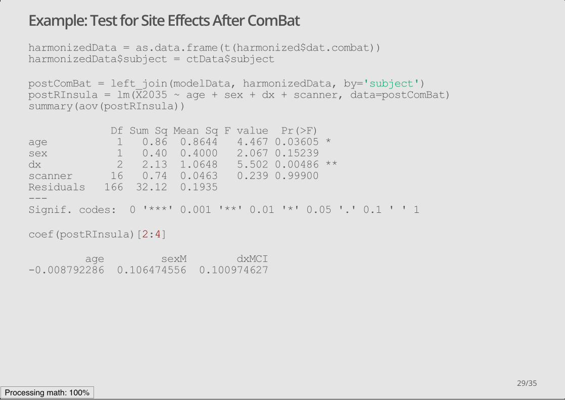
Example: Test for Site Effects After ComBat

harmonizedData = as.data.frame(t(harmonized$dat.combat)) harmonizedData$subject = ctData$subject

postComBat = left_join(modelData, harmonizedData, by='subject') postRInsula = lm(X2035 ~ age + sex + dx + scanner, data=postComBat) summary(aov(postRInsula))

Df Sum Sq Mean Sq F value Pr(>F) age 1 0.86 0.8644 4.467 0.03605 * sex 1 0.40 0.4000 2.067 0.15239 dx 2 2.13 1.0648 5.502 0.00486 ** scanner 16 0.74 0.0463 0.239 0.99900 Residuals 166 32.12 0.1935 Signif. codes: 0 '***' 0.001 '**' 0.01 '*' 0.05 '.' 0.1 ' ' 1

coef(postRInsula)[2:4]

age sexM dxMCI 0.008792286 0.106474556 0.100974627


Conclusions

Data harmonization is an important step in any image analysis that combines datafrom different sites and/or scanners.

ComBat has been successfully applied to DTI and cortical thickness data to removescanner effects while preserving biological associations of interest (Fortin et al. 2017,2018).

To obtain valid statistical inference in downstream analyses, uncertainty in ComBatharmonization should be considered

·

·

ComBat code is located at https://github.com/Jfortin1/ComBatHarmonization

Available in R and MATLAB

-

-

·


https://github.com/Jfortin1/ComBatHarmonization

Wrap-up

We’ve covered all (or most) image pre-procssing steps in a typical image pre-processing pipeline, starting with raw nifti images.

Everything was done in R!

·

·


What we didn’t cover

fMRI: see fmri library

Other imaging modalities, e.g., CT, PET

Voxel-wise testing: see voxel library

Other population-level statistical inference:

Statistical/machine learning: see caret library

·

·

MALF segmentation is robust-

·

·

·


What can you do next?

Resources

Further modeling and statistical analysis.

Register images to a template to do population inference.

General R

·

·

·

Build your own R libraries for image analysis.

Rmarkdown for reproducible reports

R shiny apps

-

-

-

Neurohacking tutorial on Coursera

Neuroconductor: central repository for image analysis R libraries

·

·


Website

http://johnmuschelli.com/imaging_in_r


ReferencesDas, Sandhitsu R, Brian B Avants, Murray Grossman, and James C Gee. 2009. “Registration Based Cortical ThicknessMeasurement.” 45 (3). Elsevier:867–79.

Fortin, Jean-Philippe, Nicholas Cullen, Yvette I Sheline, Warren D Taylor, Irem Aselcioglu, Philip A Cook, Phil Adams,et al. 2018. “Harmonization of Cortical Thickness Measurements Across Scanners and Sites.” 167.Elsevier:104–20.

Fortin, Jean-Philippe, Drew Parker, Birkan Tunc, Takanori Watanabe, Mark A Elliott, Kosha Ruparel, David R Roalf, etal. 2017. “Harmonization of Multi-Site Diffusion Tensor Imaging Data.” 161. Elsevier:149–70.

Johnson, W Evan, Cheng Li, and Ariel Rabinovic. 2007. “Adjusting Batch Effects in Microarray Expression Data UsingEmpirical Bayes Methods.” 8 (1). Oxford University Press:118–27.


image harmonization - about

Documents