image segmentation and matching using the binary object forest

Image segmentation and matching using the binary

object forest

David Nichol* and Merrilyn Fiebig’

This paper examines a robust method of image disparity analysis based on matching features derived from a graph theory technique of image segmentation. It is aimed partic~iar~y at tracking objects which exhibit large interframe motion. The approach proposed involves using multiple thresholds in an image to obtain a set of binary ‘slices’. These are processed to find all connected elementary regions in each slice. The topological relationships between aIf elementary regions (‘binary objects’) can be described bv a set of trees. This set of trees constitute the binary object forest (BOF) for a given image. After appl_ving this segmentation procedure to each image in turn, matching is performed between features (nodes) in the resulting BOFs to identify areas of change and then to extract moving objects.

Keywords: d~spar~ty analysis, ~oresponden~e, motion detection, image segmentation

INTRODUCTION

The present paper addresses the correspondence aspect of image disparity analysis. This problem is concerned with identifying which parts of one image correspond to which parts of another. It arises particularly when images are acquired as a time sequence, and it is desired to analyze temporal changes. Such changes may be due to sensor motion or to object motion or to both. The topic of especial interest in the present discussion is the detection of objects which have moved a large distance between frames of the image sequence, but the techniques described have wider application. Disparity analysis is a very active area of research but, in general, the matching techniques fall into either gradient or feature-based methods. Examples if the former are

*Information Technology Division, Electronics Research Labora- tory, ‘Optoelectronics Division, Surveillance Research Laboratory. DSTO, Salisbury. SA 5108. Australia

Pqwr received: 15 ~~~~~s~ I&W. Revised paper received: 2f Ja~~ar.v 1941

given in References 1 and 2, and the latter in References 3,4 and 5. In the case of the latter (but not the former), preliminary feature extraction is performed on the images to be analyzed and matching is attempted between the resulting features. Thus any such approach involves an extraction and a matching phase. If the features selected correspond to objects, or parts of objects, in the physical world then information about object and sensor motion is derivable from the extracted disparity vectors. (A line drawn from the centre of a feature in one image to the centre of the corresponding feature in the second is called the disparity vector for that feature). If sufficient vectors are obtained on a rigid object then the three dimensional motion of the object is estimable”. The binary object forest (BOF) technique discussed below falls into the feature based category of disparity analysis. However, feature extraction in this approach involved a complete image segmentation and the features used are elementary connected regions (binary objects or atoms) which arise during segmentation. The binary object forest is the set of trees which arises when (dyadic) topological relationships between atoms are described in graph form. Feature matching is performed by comparing nodes of the BOFs derived from the sequence of images to be processed and disparity vectors are drawn between the centroids of the corresponding BOF vertices. It is shown that simple matching rules, together with a local smoothness constraint, are sufficient to track objects which have moved large distances (100 pixels or more) between adjacent frames. This is achieved consistently even when the objects are moving against complex backgrounds. Obviously, this segmentation technique is low level in the sense that no image content (semantic) information is used in extracting features. In this way it is similar to the region adjacency graph (RAG) approach to analyzing single images”-’ ’ Other similar- ities are discussed below. Many other feature matching methods also use some graph theory formalism (e.g. References 12-14, 21), but these are typically higher level (using surface orientation, or primitive shapes for example) than the present method. High IeveI extrac-

0262-8856/93/003139-11 0 1991 Butterworth-Heinemann Ltd (subject to Crown 0)

vol9 no 3 june 1991 139

tion results in fewer feature but other, extra-image, information must be used in the process which is generahy much more complex. The BOF technique does not need any prior knowledge of the image and thus is very general. The penalty for this is that the number of nodes in the BOF (as in the RAG) can be large. Typically a 512~512 image yields ~0~0 vertices. Nevertheless it is shown that, provided suitable data structures are employed, even BOFs as complex as this can be handled quite easily to produce the required matching. In the discussion below a comparison is made with two well-known feature matching methods using example images showing large motion disparity. It is shown that the BOF technique is significantly more effective and robust than the other methods on these images. Additionally, it is shown that, despite the large number of vertices in the derived BOFs, the total processing time is Sig~ificantIy less than for the other methods. Finally, it should be noted that as the BOF segmentation of an image is complete, in the sense that every pixel is assigned to a region, then the technique may well be applicable to other image analysis problems which require region segmentation.

OUTLINE OF BINARY OBJECT FOREST DISPARITY ANALYSIS

A schematic outline of BOF segmentation is shown in Figure 3. The method involves ‘slicing’ each input image into a series of binary images (one for each threshold used). Similar multi-level thresholding is quite common in microscopy’“*‘” though this usually involves two thresholds per slice (‘density slicing’). An

(* inttialise *)

Input image f of size MxN Set initial values k := 0, label := 0

DOWHfLEk<K+l BEGIN

(I slicing *)

stage 1

Stage 2 Stage 3

Stage 4

Stage 5

Slice fusing threshold f3 k to binary image W(k)

Find and label connected objects in W(k)

Transfer label information to label map Map(k)

T’J

+ (*tindSST*}

For each object A ( label j ) get location (x, y) of any pixel in A If A is a l-object put j* := Map(k), if A is aO-object j*= Map(k-1) SubSetb] := j* This determines the subset are. Repeat until all object subset relations are found

I

k:=k+I

END

Extraction of binary object forest

Figure 1. The overall scheme for extraction of the binary object forest

140

example of slicing using four single thresholds on an aerial photograph is shown in Figure 2. Each binary image is searched for connected regions ~binary objects’ or ‘atoms’) of constant truth-value (1 or 0). Each binary object found is iabelled and information about its position, area, grey-level, etc., recorded. Topological information, such as object enclosure in a given plane and subset relationships between adjacent slices, is also obtained, and it will be shown can be compactly stored as a number of trees which together constitute the binary object forest (BOF).

The proposed disparity analysis involves determining the BOF of each two images from a sequence and then trying to match subgraphs of one with subgraphs of the other. If matching subgraphs are found corresponding to part of a moving object visible in both images then information about object motion is obtainable. Each matching vertex yields a provisional disparity vector in a motion analysis plot. Such plots are obtained as follows. If the centroid of binary object A in Image 1 is (xn, yA) and the centroid of the matching binary object B in Image 2 is (xg, yB) then a disparity vector is drawn between (,xAr yil) and (x B, yH) in the motion analysis plot.

In the following discussion the segmentation/feature extraction phase of processing is described first. This involves finding the binary objects in each thresholded image, describing the topological relationships between binary objects in the same binary image and describing the subset relations between objects in adjacent images. In the feature matching phase a search is made for matching atoms/vertices in the BOFs of each image pair. Conflict resolution and local smoothing may be needed to reduce multiple and erroneous matching.

BINARY OBJECT EXTRACTION

In this section the preliminary processing to extract elementary connected regions is described. These correspond to stages 1 to 3 of the overall scheme as shown in Figure 2.

Image slicing

Suppose the original image is sampled at M x N points (M and N are positive integers) on a domain D, and is represented by a function p(x).

If image slicing is performed at K thresholds (A,, AZ, . . . hk, . . , AK), where A, <AZ<. . . <Ak. . . <A,, then this process maps the input image f(x) into K binary valued images W,(x), Wz(x), . . ., Wk(x), . . . W,(x) such that:

W,(x) = 1 if f(x)2Ak

= 0 otherwise. (1)

For convenience the binary image corresponding to slicing at level Ak will be referred to as ‘slice k’ of f(x). It will also be convenient to make two further slices, W<,(x) and WK+i(x), which contain all OS and all Is respectively. The corresponding thresholds are to some extent arbitrary but must be such that

A,df(x) andAK+l > f(x) for all x E Df (2)

image and vision computing

I

Figure 2. Binary slices corresponding to thresholds 100, 115, 130 and 145 in an 8 bit image

As noted in the feature matching section below, the actual thresholds used were obtained by setting them to be equally spaced within +2 standard deviations of the mean. For the sort of imagery to be discussed this was entirely satisfactory. For attempting to match radically different forms of images, for example radar and infrared, a similar choice of threshold has been found to be satisfactory provided that matching is permitted between objects in different slices.

Binary objects

Informally. we have defined a binary object as a connected region of constant truth value. To be

~019 no 3 june 1941

connected pixels must be neighbours and have the same truth value. As far as neighbourhood is concerned the usual practice of defining the pixel neighbours ofx to be the set (y~O<~x-y~<2} will be followed. This definition allows diagonal as well as orthogonal neighbours which can lead to a non-planar region adjacency graph r. To avoid this a further rule is used whereby diagonals between pixels of value I are given prece- dence over diagonals with pixels of value 0.

Binary object labelling

After slicing ail images are searched for binary objects and each object found is given a unique iabie, In the

141

present implementation the search is made from slice 0 to slice K+ 1 and within each slice searching is left-to- right, top-to-bottom”. The labels are simply the natural numbers 1, 2, 3, . . ., assigned in the same order as the objects are encountered. If the image is displayed with x increasing from left to right and y increasing from top to bottom then it is possible to define an index function for object A of the form:

@A = k~~+y~~+x~ (3)

where k is the slice where object A is located and x = (x,, yA) is the top leftmost pixel of A. In Appendix 1 it is shown that this index function is useful in speeding up the extraction of enclosing relationships.

REGION ENCLOSURE TREE

This section corresponds to stage 4 of Figure 2. We are now in a position to consider the relationships between objects in each binary image slice W. The most obvious relationship is u~~uce~cy which can be defined thus:

Definition 1. Two objects A and E (in the same slice) are adjucent if there exists a pixel x belonging to A and a pixel y belonging to B such that x and y are neighbours.

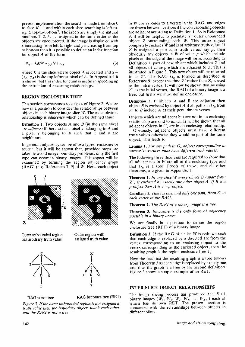
In general, adjacency can be of two types: enclosure or touch”, but it will be shown that, provided steps are taken to avoid image boundary problems, only the first type can occur in binary images. This aspect will be examined by forming the region adjacency graph (RAG) (e.g. References 7, 9) of W. Here, each object

Outer unbounded region has arbitrary truth value

B -A-F

/I\ CDG

I C D G

1 E

RAG is not tree RAG becomes tree (RET)

Figure 3. If the outer unbounded region is not assigned a truth value then the boundary objects touch each other and the RAG is not a tree

Outer region with assigned truth value

142

in W corresponds to a vertex in the RAG, and edges are drawn between vertices if the corresponding objects are adjacent according to Definition 1. As in Reference 9, it will be helpful to postulate an outer unbounded object 2 surrounding each W. This outer object completety encloses Wand is of arbitrary truth-value. If Z is assigned a particular truth value, say p, then obviously any objects in W of value p which include pixels on the edge of the image will form, according to Definition 1, part of new object which includes Z and all objects of value p which are adjacent to Z. This is illustrated in Figure 3. This new object will be referred to as Z’. The RAG G, is formed as described in Reference 9, except this time Z’ rather than Z, is used as the initial vertex. It will now be shown that by using Z’ as the intial vertex, the RAG of a binary image is a tree; but firstly we must define enclosure.

munition 2. If objects A and B are adjacent then object B is enclosed by object A if all paths in G, from Z’ to B include A as their penultimate vertex.

Objects which are adjacent but are not in an enclosing relationship are said to touch. It will be shown that all adjacent objects in G, are in an enclosing relationship.

Obviously, adjacent objects must have different truth values otherwise they would be part of the same object. This leads to:

Lemma 1. For any path in G, objects corresponding to successive vertices must have different truth values.

The following three theorems are required to show that all adjacencies in W are all of the enclosing type and that G, is a tree. Proofs of these, and all other theorems, are given in Appendix 1.

Theorem 1. In any slice W every object B (apart from Z’) is enclosed by exactly one other object A. If B is a p-object then A is a =p-object.

Corollary 1. There is one, and only one path, from Z’ to each vertex in the RAG.

Theorem 2. The RAG of a binary image is a tree.

Theorem 3. Enclosure is the only form of ffdjacency possible in a binary image.

We are finally in a position to define the region enclosure tree (RET) of a binary image.

Definition 3. If the RAG of a slice W is redrawn such that each edge is replaced by a directed arc from the vertex corresponding to an enclosing object to the vertex corresponding to the enclosed object, then the resulting graph is the region enclosure tree T,.

Now the fact that the resulting graph is a tree follows from Theorem 3 as each edge is replaced by exactly one arc; thus the graph is a tree by the second definition. Figure 3 shows a simple example of an RET.

INTER-SLICE OBJECT RELATIONSHIPS

The image slicing process has produced the K-t 1 binary images (W& WI, W2. W,, . . . , W,,,) each of which has its own RET. The present section is concerned with the relationships between objects in different slices.

image and vision computing

< 82 < 03

Key: l-object 0 O-object QQ

w” I i

5 i 5’ i i i ‘:\iJ” A F D W K+l

O-object subset tree 1 -object subset tree

Figure 4. As the threshold 0 is increased l-objects will shrink and O-objects expand

Theorem 4. The set of pixels representing each p-object in slice W,, where 0 <k < K + 1, is the subset of a set of pixels representing a p-object in either W,_, (for l-objects) or W, +, (for O-objects).

This situation is illustrated in Figure 4. It is now possible to form the object subset graphs of the image f(x). The l-object subset graph is obtained by forming a graph with vertices corresponding to all l-objects in the set of K + 2 slices and drawing directed arcs from each object to subset objects in the higher threshold adjacent slice. Obviously no arc will be drawn from W,,, as there is no higher threshold slice. Similarly the O-object subset graph is formed by drawing arcs between objects and their subset objects in lower slices. No arcs will be drawn from Wo, as there is no lower slice. In Appendix I the following theorem is proved:

Theorem 5. The O-object subset graph and the l-object subset graph are both trees.

Figure 4 shows a simple example of such subset trees.

BINARY OBJECT FOREST

It has been shown that the topological relationship between binary objects in a single slice can be described by the region enclosure tree. It was also shown that the subset relationships between objects in adjacent slices can be described by the object subset tree (OST). Thus an image f(x) thresholded into K + 2 slices can be described by K + 2 region enclosure trees and 2 object subset trees (one for each type of object).

In Stage 5, the subset tree relationship is determined. After each Stage 3, the object labels are entered into a label map which is a two dimensional array of size Mx N. Thus to find which object a given pixel in slice W has been assigned to, examine the corresponding element in this map. Beside the current map, the label map for the previous slice is also retained for Stage 5 processing. From Theorem 4 it follows that each l-object in the current map will be the subset of a l-object in previous map, and vice versa for O-objects. Thus, if in Stage 3 the location of a single pixel (the top- left say) had been saved for each object, then by examining the same pixel in the relevant adjacent label map the subset arc can be identified. Thus by tempor- arily retaining the subset maps of the current and prior slices the subset tree can be readily extracted.

FEATURE MATCHING

Defintion 4. If an image f(x) is thresholded into K + 2 As mentioned, the approach used is to obtain the BOF slices then the graph consisting of the K + 2 region of each of a pair of images taken from a sequence and enclosure tree plus the 2 object subset trees is the to then try to match various substructures in each of the binary object fore.yt (BOF) of f(x). resulting graphs. Figure 5 illustrates the general prin-

IMPLEMENTATION

Extraction of the BOF is comparatively straightfor- ward. Essentially, this is because all relationships are described by trees, and thus each binary object is only enclosed by a single object and is the subset object of only one object. Thus the BOF is completely specified by finding these two arcs for each object-vertex and then storing them in a suitable structure. It will be shown that the extraction and storage process can be achieved by sequentially slicing the image and record- ing the relationship within in each slice and between one adjacent slice.

Figure 1 shows the overall schema used to extract the BOF. After reading in the raw image in Stage 1 image slicing is performed, at threshold hk, in Stage 2. This produces a binary image W(k). During Stage 3 binary objects are detected, labelled and various object parameters measured and recorded. This information is stored in one dimensional arrays such that the value of a particular parameter X for the object labelied i is given by the ith element of the array. The actual parameters measured depend on the application but typically will include object area. x and y centroid and other basic statistics. Housekeeping information, for use in later stages, is also stored in Stage 3. For example, the x and y coordinates of the top-left pixel of each object are saved for use in Stage 5.

The RET is determined in Stage 4. As mentioned above, it is only necessary to find a single arc for each object A to specify the RET completely. This arc is easily found as it is the arc (AB) drawn from A to the (unique) adjacent object B which has a label less than that of a. This follows from:

Theorem 6. If the set of adjacent objects to object A has labels L= {i,, iz, i3, . .} then the object B which encloses A is the only object in L which has a lower label than A.

The proof of this is given in Appendix 1. Once this has been performed for each object in a given slice the RET for that slice is determined completely. This process is repeated for each slice.

vol9 no 3 june 1991 143

G H C D

well be produced by random noise. Empirically it was found that MinSize = 4 (pixels) resulted in a satisfactory ratio of good-to-bad matches. R2 Same threshold: as the lighting conditions did not change much during the typical sequences used it was possible to reduce the search time considerably by trying only to match objects generated by the same threshold. However, as the thresholds were chosen to be equally spaced within f2~r of the image mean then some immunity to changing light levels is obtained automatically. As previously mentioned, for a radically different pair of images matching between different threshold objects may become necessary. Typically, 8 thresholds were used. R3 Upper bound on area differences: matching is not attempted if differences in area between objects was greater than 15%. R4 Maximum shift: searching a larger area for matching obviously increases the risk of erroneous matches. However, for the cases of interest large

Level 2 Region 5 Enclosure Trees

t A

Figure 5. This shows the RETs produced by slicing each image from a pair at a given threshold. The proposed feature matching involves finding corresponding substructure in the various trees of the BOF. In this case the object CAR is described by the subtree (BCD) in one slice and by (FGH) in the second

cipal involved. This shows the RETs which results from slicing the image pair at a single threshold. The subgraph with vertices label list (B CD) in Image 1 represents the same physical object as the list (FG H) in Image 2. One of the attractions of BOF analysis is that such substructure is more or less independent of the background and, because only topological relationships are described, they have a high degree of robustness to scale and rotation, as well as translation. There are various possible substructure matching strategies but only the simplest case, vertex matching, is considered in the present discussion. For example, in Figure 5 searches are made for matches between individual vertices of the two trees. The fact that, besides the individual matches BIF, CIG and DIH, there is also a higher level match between (B C)I(FGH) is used only implicitly in the postprocessing smoothing stage where isolated matches are rejected. BOF analysis on a typical 512 x 512 8 bit image will yield 10000 binary objects for 8 thresholds. Obviously, trying to match each of the corresponding set of 10000 vertices will be time consuming. To reduce such time penalties a set of rules is used to suppress matching attempts which are unlikely to succeed. The rules used, together with typical parameter values, are:

Rl Minimum area: objects smaller than MinSize are not considered. The idea here is to reduce the search time by not considering objects which may

Figure 6. Image pair A. The target object has moved approximately 100 pixels between frames

144 image and vision computing

movements were expected so this limit was set very large (typically several hundred pixels). No minimum shift was specified.

Provisional matches between the two sets of vertices were made if the pair of vertices pass Rl to R4. These matching rules were deliberately kept simple to mini- mise processing time. Generally, however, this leads to some mismatches. The following additional rules were used to suppress these:

R5 Conflict resolution: if two or more similar matches from an object in the first frame to objects in the second frame are obtained then resolve this by comparing local correlations over a small area (5 X 5) for each possible match. R6 Local smoothness: in the first phase of this rule, disparity vectors are removed if they are isolated. The text used is that a similar vector must be found whose head and tail are less than n, pixels from the candidate vector. This test distance n, was typically

Figure 7. Image pair B. Both objects have moved approximately IO0 pixels between frames

10 pixels. In the next phase vectors are removed if they were not of similar length and direction to the majority of other vectors chosen by the same distance test. Only a weak test of ‘similarity’ was used; typically this was that x and y components be within +.5 pixels.

Of course, many other, more complex, matching rules (using shape or BOF substructure for example) could be used; however, it was found these simple ones gave very satisfactory results for a wide range of images. More complex rules would obviously require more processing time.

EXAMPLES

The BOF matching technique has been applied success- fully to many different types of images. Figures 6 and 7 show examples of images used. These were obtained by directly digitizing the output of a video camera viewing a scene. Figure 6, which will be referred to as Pair A, is an outdoor scene containing a single moving object a significant distance in a moderately complex background. Figure 7 (Pair B) is a tabletop scene showing two moving objects. The background is simple but as

Figure 8. Disparity vectors found between frames for image pairs A and B using BOF matching. Only one erroneous vector is found

vol9 no 3 june 1991 145

well as translational motion there is significant motion towards the camera.

Slicing was performed on each of the 8 bit image pairs using 8 equally spaced thresholds between _+Za about the mean greylevel. This yielded 8760 atoms in Pair A and 5795 atoms in Pair 3. As well as enclosure and subset relationships, parameters describing,object truth value, centroid, threshold, area, euler number and so on were stored as previously described. Match- ings were performed between the BOF vertices according to the above rules (and parameter values). Figure 8 shows the disparity vectors in a motion analysis plot obtained using the above rules on the BOFs derived from the image Pairs A and B. For comparison with existing techniques these images have also been processed using the well known Barnard and Thompson algorithm’ and one developed by Prazdn lg. Both these use the Moravec interest operator 2X to find locally complex regions which are likely to be suitable for matching. Figures 9 and 10 show the disparity vectors obtained using these two methods on the example image pairs. There are of course various parameters in both these methods which could be

Figure IO. disparity vectors found between frames for image Pairs A and B using the Prazdny algorithm. zany correct matches ark made for both moving and stationary objects. However there are also a number of grossly erroneous vectors

Figure 9. Disparity vectors found between frames for image Pairs A and B using the hazard and Thompson algorithm. Although many correct background vectors were found there were oniy a few on the moving objects

changed; the examples shown use the values which were found to give the best results on these images.

To try to compare objectively the different algor- ithms all disparity vectors obtained for each method on each image pair were classified as either correct/target, corre~t/background or erroneous. For the first two categories the ‘correctness’ was determined by comparing the computed displacement with the estimated target shifts determined using interactive techniques. It is estimated that these measured vectors were accurate to the nearest two pixels. To allow for measurement errors a latitude of zt2 pixels was alowed for target vectors. There was little movement in the backgrounds due to camera jitter, wind and similar effects. To allow for this, and also to ease the burden of scoring, background vectors of three or less pixels were scored as ‘correct’. All vectors which did not meet these criterion were classified as ‘erroneous’. Table 1 shows the results of such analysis on image pairs A and B.

The number of correct target vectors found by the BOF technique was adequate for both image pairs. The parameter values used for both image pairs were the


Table 1. Disparity vector classification

Pair

A A A

A A A

B

B

B

Method/set number Total vectors Correct/target Correct/background Erroneous

Prazdny 1 274 6 249 19 Prazdny 2 238 6 220 I2 Prazdny 3 213 5 197 11

Bamard/Thompson 1 198 0 198 0 Barnard/Thompson 2 464 0 464 0 Barnard/Thompson 3 202 2 198 2

BOF I 174 7 167 0

Prazdny 4 147 45 81 27

Barnard/Thompson 4 281 6 260 IS

BOF 2 86 33 52 I

default values given in Rl-R6. As previously mentioned? the minimization, and preferably the eiimina- tion, of rogue vectors is an extremely important requirement for disparity analysis. From this viewpoint the BOF algorithm performed very well for both A and B with only one error produced. The total number of matches found was somewhat less for this method than for the other techniques. However, the number of erroneous vectors accepted was considerably less.

Using the recommended parameters’ the Barnard and Thompson algorithm performed perfectly, in the sense of not producing erroneous vectors, for Pair A. However, no target vectors were found in either image using the recommended parameters. The row of Table 1 listed as ‘Barnard/Thompson 1’ corresponds to these parameters for A. It was thought that this problem might be due to insufficient interest points falling on the vehicle. If so then initial matches found might be removed during the recursive matching refinement process (equivalent to the ‘local smoothness’ Rule of the BOF). To test this the number of interest points requested was increased to 2000 for A but as can be seen in Table 1 (‘Barnard/Thompson 2’) this still yielded no vectors on the moving object. To achieve the vectors shown in Figure 8 (‘Barnard/Thompson 3’ and ‘Barnard/Thompson 4’) it was necessary to reduce the parameter c. used in assigning initial probabiIities, from the recommended value of 10.0 to 0.00001 (many intermediate values were also tested). However, as can be seen in Figure 9, this reduction also produces erroneous vectors.

The method of Prazdny also uses the Moravec interest points as an initial step. In A an adequate number of moving object matches were made but at the expense of a significant numbers of erroneous matches. This problem was reduced somewhat by increasing the a priori minimum probabilities from the recommended 0.2 to 0.5 to 0.9. These correspond to ‘Prazdny l’, ‘Prazdny 2’ and ‘Prazdny 3’. ‘Prazdny 4’ used the value of 0.9 on B. A large number of correct object vectors was found, though once again at the cost of significant erroneous vectors.

Finally. it is worth noting that in terms of CPU processing time the BOF technique was considerably faster than the other two methods. Obviously algorithm timings depend very strongly on their implementation but as the CPU times involved for the BOF, Prazdny and Barnard and Thompson methods were found to be (approximately) in the ratio of 1:4:10 then this differ- ence is probably significant.

v&Y no 3 june $991

CONCLUDING REMARKS

The binary object forest technique appears to be a useful approach to the image disparity analysis problem, especially for the case of image pairs exhibiting large interframe object motion. The method seems to be robust with little or no change in parameters required between different image types. It is also worth noting that as the vertex matching scheme described above basically used only areas and intensities for comparison there is considerable ‘reserve power’ in the BOF method. If certain types of images generate too many false alarms using these basic criteria then more complex matching, using shape measurements for example, could be invoked. Also, in view of the success of single vertex matching, it has not been necessary to explore the advantages of matching high order substructure in the present paper. For images containing many moving objects which change scale radically between frames (for example due to significant motion along the sensor-object axis), it may well be desirable to match substructures consisting of several vertices and arcs. Potentially this could lead to the minimizing of false matches without the use of postprocessing techniques such as smoothing. This aspect is explored in a subsequent paper”.

ACKNOWLEDGEMENT

We would like to thank our colleague, Janet Aisbett, for the very useful discussion concerning interpretation of the algorithm comparison experiments.

REFERENCES

1 Nagel, H-H ‘Displacement vectors derived from second-order intensity variations in image sequences’ Comput Vision Graph. & Image Pro- cess. Vol 21 (1983) pp 85-117

2 Horn, B and &hunk, B ‘Determining optical flow’, Ariifbztell. Vol 17 (1981) pp 185-203

3 Grimson, W E L ‘Binocular shading and visual surface reconstruction’, Comput Vision Graph. & Image Process. Vol 28 (1983) pp 19-43

4 Price, K E ‘Relaxation matching techniques - a comparison’, IEEE Trans. PAMI Vol 7 (1985) pp 617-623

5 Barnard, S T and Thompson, W B ‘Disparity analysis images’, IEEE Trans. PAMI Vol2 (1980) pp 333-340

147

6

7

8

9

10

11

12

13

14

15

16

17

18

19

20

21

22

Adiv, G ‘Determining three-dimensional motion and structure from optical flow generated by several moving objects’, IEEE Trans. PAMZ Vol 7 (1985) pp 384-401 Pavlidis, T Structural Pattern Recognition Springer-Verlag, Berlin (1977) Feldman, J A and Yakimovsky, Y ‘A semantics- based region analyser’ Artif Zntell. Vo15 (1973) pp 349-371 Niehol, D G ‘Autonomous extraction of an eddy- like structure from infrared images of the ocean’, IEEE Trans. Geoscience and Remote Sensing Vol 25 (1987) pp 28-34 Nichoi, D G, Fiebig, M J, Whatmough, R J and Whitbread, P J ‘Some image processing aspects of a military geographic information system’, Austra- lian Computer J. Vol 19 (1987) pp 154-160 Nichol, D G ‘Region adjacency analysis of remotely sensed imagery’ ht. J. Remote Sensing (1990) Jacobus, C L, Chien, R T and Selander J M ‘Motion detection and analysis of matching graphs of intermediate-level primitives’, IEEE Trans. PAMI Vo12 (1980) pp 495-510 Gu, W K, Yang, J Y and Huang, T S ‘Matching perspective views of a 3-D object using circuits’, Prnc Seventh Int. Conf Pattern Recognition Vat 1 (1984) pp 441-443 Bertold, M and Long, P ‘Graph matching by parallel optimization methods: An application to stereo vision’, Proc. Seventh Int. Conf. Pattern Recognition Vol 2 (1984) pp 841-843 Preston Jr., K ‘Gray level processing by cellulat logic transforms’, IEEE Trans. PAMI, Vol 5 (1983) pp 55-58 Ripley, B D Spatial Statistics Wiley, New York, NY, USA (1981) Aisbett, J E ‘Optical flow with an intensity weight- ed smoothing’, IEEE Trans. PAMI Vol 11 (1989) pp 512-522 Berge, C Graphs and Hypergraphs North- Holland, Amsterdam, Netherlands (1973) Prazdny, K ‘Egomotion and relative depth map flow from optical flow’, Biological Cybernetics Vol 36 (1980) pp 87-102 Moravec, H P ‘Towards automatic visual obstacle avoidance’, Proc. Fifth Int. Joint Conf. on Artif. Intell. (1987) p 584 Boyer, K L and Kakm, AC ‘Structurai stereopsis for 3-D vision’, IEEE Trans. PAMZ Vol 10 (1988) pp 144-166 Nichol, D G and Fiebig, M J ‘Tracking multiple moving objects by binary object forest segmentation’, submitted to Image & Vision Comput. (1990)

APPENDIX 1

Theorem 1. In any slice W every object B ~apart from 2’) is enclosed by exactly one other object A. If B is a p-object then A is a =p-object.

Proof. Consider a p-object B in slice W (see Figure Al). A pixel x of B is said to form part of its outer boundary if a path, which does not include any other pixel of B can be drawn from any x to any pixel of Z’.

Proof. It will first be shown that a path exists between 2’ and any vertex B. Consider an arbitrary walk between Z’ and B. This can be found, for example, by drawing a line in W from a pixel of Z’ to a pixel of B and noting which objects are traversed. Suppose this walk is ,u = (Z’, C,, C,, . . . C,,, B). NOW the Ci are not necessarily distinct but this walk can be turned into a path by the following method:

Starting from Cr, move along the walk noting the first and last occurrence of each vertex. If a vertex occurs once only then leave the vertex unchanged. Otherwise, remove the sequence of vertices between the first up to, and including, the last occurrence of a vertex. This new walk p”’ is clearly connected and each vertex occurs only once; it is thus a path which completes the first part of the proof.


: . ..“.,;

‘. .: :.: ., ,.,.

.’ : ...... ; ,..y,

: ::, . ..I... . . : . . . :.

:, ..

:

:. :

.:.

.:

Z :,:. ,,,

. . :

P Figure Al. Ail paths to a p-object B from Z must pass through a connected set of =p-pixels. As these pixels are connected they must form part of an enclosing =p-object A. This object is obvio~ly unique. Path Y to B from Z must include A. q : p-object; 0: p-object (partial); Cl: unspecified; Cl: unbounded

Now the pixels of B which form its outer boundary are clearly connected and of truth-value p. Consider the set of pixels which are adjacent to, but ‘outside’, this boundary. (A pixel y is outside B if a path can be drawn to any pixel in 2’ without including a pixel from B). These are all of truth-value =p and are connected. Thus from Definition 1 they must be part of a single object, say A. Obviously, at1 paths to B must include A as the penultimate object and A must, by definition, enclose B. This process can be repeated for all objects in W, including boundary objects which are either part of, or enclosed by, Z’, and the Theorem follows. q

Corollary 1. There is one, and only one path, from Z’ to each vertex in the RA G.

From the above discussion it follows that a path ,u~ = (Z’, A,, A2, . . . A,, B) exists from Z’ to any vertex B. From Theorem 1 and Definition 3 it follows that B must be enclosed by A, and only by A,. Similarly, A,_, is the only object that encloses A,. Repeating this process for each preceding vertex shows that ,u~ is unique, which proves the Corollary. q

Theorem 2. The RAG of a binary image is a tree.

Proof. The standard defintion of a tree is that it is connected graph without cycles”. Now it has been shown that a path exists from Z’ to each vertex of G,, and thus G, is connected. Suppose a cycle (B, C,, C2, . ., C,,, B) exists in G, where m> 1 (by defintion of a cycle). Consider the path ,UC, from Z’ to Ci (I did m). Now as each vertex, apart from the first, of a cycle is distinct then the paths FB = (,u,-, C;+,, . . ., C,,, B) and ,u’,, = (C;, C1_,, . . ., C,, B) must be both legitimate and distinct. But this implies there are two paths from Z’ to B which contradicts Corollary 1. Thus no cycles can exist in G, and the RAG must be a tree. 0

Theorem 3. Enclosure is the only form of adjacency possible in a binary image.

Proof. An equivalent definition of a tree to the one above is that it is a graph with no cycles and NW- I arcs. where NW is the total number of vertices’s. As it has been proved that G, is a tree, then this must also hold. Now from Theorem 1 each object of W, except Z’, is enclosed by exactly one object. As enclosure implies adjacency there are thus NW- 1 corresponding edges of G,,. Thus there cannot be any other edges, or adjacencies. corresponding to the non-enclosing kind. Cl

Theorem 4. The set of pixels representing each p-object in slice W,, where 0 < k < K + 1, is the subset of a set of pixels representing a p-object in either r;V,_, (for I-objects) or W,,, (for 0 objects).

Proof. Suppose object Ak is a l-object in slice Wk and this consists of K’ pixels Ak = {x,, x2, x3, . . ., xKsf. From the above it follows that f(xk,‘) 3’Ak for all xk. E A,. Now as A >A&] then this will certainly hold for the same pixels in slice W,_, . Obviously, the object connectivity requirements must also hold in Wk_,, but as the threshold has been lowered there may be additional pixels in w&i which are connected to pixels of the set Ak. Thus the original set of pixels, and any extra pixels which meet the connectivity and threshold requirements of Definition 1. will form a l-object Ak_, in W,_, Clearly. A,, C-Ax_, and the Theorem follows for l-objects.

A similar argument, but considering slice Wk+,, proves the theorem for O-objects. •i

Theorem 5. The O-object subset graph and the l-object subset graph are both trees.

Proof. Consider any l-object Ak in slice ty, where O< k< K + 1 (k is chosen so that at least one l-object exists in wk). From Theorem 4 it follows that Ak is the subset Of an object Ak_i in Wk_i. Similarly, Ak_, is the subset of an object Ak-~z in W,_1. Eventually, a set of

l-objects is found such that Ak CAk_1 CAk_zC-. . . LA1 !Z W;,. From the definition of a l-subset graph arcs must exist ‘between verices corresponding to each object in this list. Thus a path (Ak. Ak-, , Ak-2, . . , A I. W,,) exists between any vertex Ali and WO. Thus the l-object subset graph is connected (and has a root W(J.

Now if the total number of l-objects is N’, then as each object except W,, is the subset of one (and only one) other object, then the total number of arcs in the graph must be N’ - 1. It follows that the l-object subset graph is a tree T’,V with root WC,.

Similarly, it can be shown that the O-object subset graph is a tree ToS with root W,,,. cl

Theorem 6. If the set of adjacent objects to object A has labels L = (i,, i2, iY, . . .> then the object B which encloses A is the only object in L which a has a tower label than A.

The proof of this follows from the following lemmas:

Lemma 2. A is enclosed by exactly one of the objects corresponding to labels in the set L = {i,, i2, i3, . . .) and encloses the remainder (if any).

Proof. From Theorem 3 it follows that A must be in an enclosure relationship with its adjacent objects. From Theorem 1 one, and only one, of these adjacent objects encloses A and hence A must enclose any remaining objects. c7

Lemma 3. Each binary object has a distinct index function 0, and if the indices of all objects found are placed in monoton~ca~[y increasing ~~eqi~en~e (8,) f&, 63, . ., di, . . , 0,) then the iih term of this sequence corresponds to the object labelled i where 1 d i S I and I is the total number of objects.

Proof. The first part is obvious as a given pixel in a given slice can only belong to one object. The second part follows as it is also clear that 0 will increase monotonically with each new object found. Cl

Lemma 4. If object A with label in encloses object B with label in then iA <in.

Proof. &IppOSe x8 = (Xg, yB) iS the top-left pixel Of B and consider the pixel x’ = (-x8, y, - 1). Now x’ cannot be in B otherwise xH would not be the top-left pixel. As A encloses B then x’ must be in A (otherwise it would be possible to generate a path from Z’ to B which did not have A as its penultimate vertex).

If XA = (XA, yA) is the top left hand pixel of A, then the index functions of these three pixels are, from equation (3):

8s= kMN+ybN+x,

0’ = kMN+yb(N- 1)+-xX,

OA = kMN~yaNix~. (Al)

As x’ is in A, then 6A6@’ and as, from (Al), 6’<8,, then it follows that N<eR, Hence, from Lemma 3.

i,<i,. (AZ)

The proof of the theorem follows immediatley. •1

vol9 no 3 june 1991 149

image segmentation and matching using the binary object forest

Documents