image segmentation and reconstruction of 3d surfaces from ... · image segmentation and...
TRANSCRIPT

Rui Antonio Henrique Fernandes da Rocha
Image segmentation and reconstruction of
3D surfaces from carotid ultrasound images.
Tese submetida aFaculdade de Engenharia da Universidade do Porto
para a obtencao do grau deDoutor em Engenharia Electrotecnica e de Computadores
Dissertacao realizada sob a supervisao doProfessor Doutor Aurelio Joaquim de Castro Campilho
e do Professor Doutor Jorge Alves da SilvaDepartamento de Engenharia Electrotecnica e de Computadores
Faculdade de Engenharia da Universidade do Porto
Julho de 2007


Dedicated to my family


ACKNOWLEDGMENTS
The author would like to thank:
Dr. Elsa Azevedo and Dr. Rosa Santos, from the Faculty of Medicine of theHospital de S. Joao do Porto, for providing most of the images and the manualsegmentations used to validate the results.
Dr. Gabriela Lopes from the SMIC (Servico Medico de Imagem Computorizada),for some of the images used in this work.
Professor Joao Sanches and Master Jose Seabra, from the Department of Elec-trical and Computer Engineering of the Instituto Superior Tecnico de Lisboa, forsharing a few 3D volumes.
Professor Aaron Fenster, from the Imaging Research Laboratories, Robarts Re-search Institute, London, Ontario, Canada, for sharing one of the used 3D volumes.
The Division of Signal and Image of the INEB (Instituto de Engenharia Bio-medica) of the University of Porto, for providing the material conditions to do thework.
My supervisors, Professor Aurelio Campilho and Professor Jorge Alves da Silva,from the Department of Electrical and Computer Engineering of the Faculty ofEngineering of the University of Porto, for their friendship, guidance, support andinspiration.

ABSTRACT
A new algorithm is proposed for the automatic segmentation of the common carotidwall in ultrasound images. It uses the random sample consensus (RANSAC) methodto estimate the most significant cubic splines or ellipses fitting the edge map of alongitudinal or a transversal section, respectively. Periodic spline fitting is also in-vestigated for transversal sections. The geometric model (spline or ellipse) consensusis evaluated through a new gain function, which integrates the responses to differentdiscriminating characteristics of the carotid boundary: the proximity of the geomet-ric model to any edge pixel and to valley shaped edge pixels; the consistency betweenthe orientation of the normal to the geometric model and the intensity gradient; andthe distance to a rough estimate of the lumen boundary.
To obtain an edge map with reduced noise and a good localization of the edges, anew robust non-linear smoothing filter was conceived. It preserves weaker intensityedges if they have low curvature, which is a common characteristic of anatomicalstructures. The smoothing filter combines the image curvature with an edge de-tector, known as the instantaneous coefficient of variation (ICOV), more suited toultrasound imaging than the intensity gradient norm. Robust statistics methods areused to improve the automatic stopping of the smoothing and to produce sharperboundaries.
For the detection of the lumen boundary, a new dynamic programming modelwas conceived for longitudinal sections and adapted to transversal sections, wherethe boundary is a closed curve. It looks for the path that maximizes the accumulatedICOV strength, previously normalized in the direction normal to the lumen axis. Ahybrid geometric active contour is also introduced. It uses a smooth thresholdingsurface and the image intensity topology to reduce some segmentation errors, left bythe dynamic programming algorithm, and to guide the smoothing of the detectedlumen boundary.
A new approach and several implementation details are investigated for the au-tomatic reconstruction of 3D surfaces of the common carotid. The surfaces arecomputed from the wall and lumen boundary contours segmented in each frame ofa data set acquired with a 3D ultrasound freehand system.
A level set algorithm is proposed for the computation of new slices from the re-constructed 3D surfaces. A cross sectional area minimization approach is introducedto compute reliable estimates of slices normal to the longitudinal axis of the carotidartery.
Statistics for the segmentation results are computed for each case, using an imagedata base manually segmented by a medical expert as the ground truth.

RESUMO
Um novo algoritmo e proposto para a segmentacao automatica da parede da carotidacomum em imagens de ultrasons. Este usa o metodo do consenso de amostraaleatoria (RANSAC-random sample consensus) para estimar os splines cubicos ouas elipses com ajuste mais significativo ao mapa de contornos de uma seccao longi-tudinal ou transversal, respectivamente. O ajuste de splines periodicos e tambeminvestigado para seccoes transversais. O consenso do modelo geometrico (spline ouelipse) e avaliado atraves de uma nova funcao de ganho, que integra as respostasa diferentes caracterısticas discriminantes da fronteira da carotida: a proximidadedo modelo geometrico de qualquer pixel de contorno e de pixels de contornos comforma de vale; a consistencia entre a orientacao da normal ao modelo geometrico eo gradiente de intensidade; e a distancia a uma estimativa grosseira da fronteira dolumen.
Para obter um mapa de contornos com ruıdo reduzido e uma boa localizacaodos contornos, foi concebido um novo e robusto filtro nao linear de suavizacao.Este preserva contornos de intensidade mais fraca se tiverem baixa curvatura, umacaracterıstica comum de estruturas anatomicas. O filtro de suavizacao combina acurvatura da imagem com um detector de contornos, conhecido por coeficiente devariacao instantanea (ICOV-instantaneous coefficient of variation), mais adequadoa imagens de ultrasons do que a norma do gradiente de intensidade. Sao usadosmetodos de estatıstica robusta para melhorar a paragem automatica da suavizacaoe para produzir fronteiras de maior contraste.
Para a deteccao da fronteira do lumen, foi concebido um novo modelo de pro-gramacao dinamica para seccoes longitudinais e adaptado para seccoes transversais,onde a fronteira e uma curva fechada. O algoritmo procura o caminho que maximizao valor acumulado do ICOV, previamente normalizado na direccao normal ao eixodo lumen. Um contorno geometrico hıbrido e tambem introduzido. Este usa umasuperfıcie suave de limiarizacao e a topologia da intensidade da imagem para reduziralguns erros de segmentacao, deixados pelo algoritmo de programacao dinamica, epara guiar a suavizacao da fronteira do lumen detectada.
Uma nova abordagem e diversos detalhes de implementacao sao investigados paraa reconstrucao automatica de superfıcies 3D da carotida comum. As superfıcies saocalculadas a partir dos contornos da parede da carotida e da fronteira do lumensegmentados em cada imagem do conjunto de dados adquirido com um sistema deultrasons 3D de maos livres.
E proposto um algoritmo baseado em conjuntos de nıvel para o calculo de novasfatias a partir das superfıcies 3D reconstruıdas. Uma abordagem de minimizacao da

x
area transversal e introduzida para calcular estimativas fiaveis de fatias normais aoeixo longitudinal da arteria da carotida.
Sao calculadas estatısticas para os resultados da segmentacao, para cada caso,usando como referencia uma base de dados de imagens segmentadas manualmentepor um medico especialista.

RESUME
Un algorithme nouveau est propose pour la segmentation de la carotide commune surimages ultrasonores. On utilise la methode du consensus a echantillons aleatoires(RANSAC-Random Sample Consensus) pour estimer la courbe spline cubique oul’ellipse qui est adaptee a carte des contours detectes sur une coupe longitudinaleou transversale, respectivement. Le consensus du modele geometrique (spline ouellipse) est evalue a travers d’une nouvelle fonction de gain qui integre les reponses adifferentes caracteristiques discriminantes de la frontiere de la carotide: la proximitedu modele geometrique a quelqu’un pixel du contour et aux pixels qui restent envallees, la consistance entre l’orientation de la normale au modele geometrique etle gradient des niveaux de gris, et la distance a une approximation grossiere de lafrontiere du lumen.
Pour obtenir une carte de contours avec moins de bruit et une localisationprecise des contours, nous avons concu un nouveau filtre de lissage non-lineaire.Il preserve les contours les plus faibles s’ils ont une courbature reduite, qui est unecaracteristique commune des structures anatomiques. Le filtre de lissage combinela courbature de l’image avec un detecteur de contours, connu par coefficient devariation instantanee (ICOV-Instantaneous Coefficient of Variation). Methodes dela statistique robuste sont utilisees pour ameliorer le critere d’arret du lissage et lanettete des contours.
Pour la detection de la frontiere du lumen, un nouveau modele de programmationdynamique a ete concu pour les coupes longitudinales et il fut adapte aux coupestransversales, ou la frontiere est une courbe fermee. Il cherche le chemin dont laforce accumulee de l’ICOV, normalisee auparavant dans la direction normale a l’axedu lumen, est maximale. Il use une surface de seuillage lisse et la topologie desniveaux de gris de l’image pour reduire quelques erreurs de segmentation, dues al’algorithme de programmation dynamique, et pour guider le lissage de la frontieredu lumen detectee.
Une nouvelle approche et plusieurs details d’implementation sont explores pourla reconstruction automatique de la surface 3D de la carotide commune. Les surfacessont calculees a partir des frontieres de la carotide e du lumen, obtenues par segmen-tation de chacune des images d’un ensemble obtenu avec un systeme d’echographie3D mode main-livre.
An algorithme base sur la methode d’ensembles de niveau zero (level sets) estpropose pour determiner de nouveaux coupes sur les surfaces reconstruites. Uneapproche de minimisation de l’aire de la coupe transversale est introduite pourobtenir des estimations fiables de coupes normales a l’axe longitudinal de l’artere

xii
carotide.Mesures statistiques des resultats de la segmentation sont calculees, ayant comme
reference un ensemble d’images qui ont ete segmentees manuellement par un medecinspecialiste.

LIST OF ABBREVIATIONS
2D - Two dimensional3D - Three dimensionalA-mode - Amplitude modeB-mode - Brightness modeCCA - Common carotid arteryCT - Computer TomographyCVA - Cerebrovascular accidentDP - Dynamic programmingECA - External carotid arteryGDM - Geometric deformable modelGVF - Gradient vector flowICA - Internal carotid arteryICOV - Instantaneous coefficient of variationIMT - Intima-media thicknessIVUS - Intravascular ultrasoundLMCE - Local minimum cross entropyMAD - Median absolute deviationMCE - Minimum cross entropyMRI - Magnetic Resonance ImagingPDE - Partial differential equationPET - Positron Emission TomographyRANSAC - Random sample consensusROI - Region of interestSDL - Signed distance to the lumen boundarySEM - Stochastic expectation-maximizationSMCE - Sequential minimum cross entropyTV - Total variation


LIST OF FIGURES
2.1 B-mode ultrasound image . . . . . . . . . . . . . . . . . . . . . . . . 72.2 Color-coded duplex sonography . . . . . . . . . . . . . . . . . . . . . 82.3 3D freehand ultrasound system . . . . . . . . . . . . . . . . . . . . . 102.4 Anatomy of the carotid . . . . . . . . . . . . . . . . . . . . . . . . . . 11
4.1 Block diagram of the approach . . . . . . . . . . . . . . . . . . . . . . 254.2 Localization of the lumen axis . . . . . . . . . . . . . . . . . . . . . . 264.3 Determination of the SDL in a longitudinal section . . . . . . . . . . 274.4 Determination of the SDL in a transversal section . . . . . . . . . . . 284.5 Edge maps produced by non-1––------linear image filtering . . . . . . 314.6 Dominant direction of the gradient . . . . . . . . . . . . . . . . . . . 334.7 Edge map cleaning . . . . . . . . . . . . . . . . . . . . . . . . . . . . 354.8 Valley edges . . . . . . . . . . . . . . . . . . . . . . . . . . . . . . . . 364.9 Segmentation with a periodic 2D spline . . . . . . . . . . . . . . . . . 414.10 Ellipse parameters . . . . . . . . . . . . . . . . . . . . . . . . . . . . 424.11 Radial carotid lines . . . . . . . . . . . . . . . . . . . . . . . . . . . . 434.12 Fuzzy functions used in the gain function . . . . . . . . . . . . . . . . 484.13 Simplex method applied to ellipses . . . . . . . . . . . . . . . . . . . 504.14 Segmented carotid walls in longitudinal sections . . . . . . . . . . . . 544.15 Segmented carotid walls in transversal sections . . . . . . . . . . . . . 554.16 Manual versus automatic segmentation . . . . . . . . . . . . . . . . . 564.17 Failures in the segmentation of the wall . . . . . . . . . . . . . . . . . 584.18 Error statistics for the wall segmentation . . . . . . . . . . . . . . . . 594.19 CPU statistics for the wall segmentation . . . . . . . . . . . . . . . . 59
5.1 Segmentation examples for the Otsu’s algorithm . . . . . . . . . . . . 655.2 Segmentation examples for the Kittler’s algorithm . . . . . . . . . . . 665.3 Segmentation examples for the Kapur’s algorithm . . . . . . . . . . . 675.4 Segmentation examples for the Sahoo’s algorithm . . . . . . . . . . . 685.5 Segmentation examples for the Yen’s algorithm . . . . . . . . . . . . 695.6 The triangle algorithm . . . . . . . . . . . . . . . . . . . . . . . . . . 695.7 Segmentation examples for the triangle algorithm . . . . . . . . . . . 705.8 Segmentation examples for the MCE algorithm . . . . . . . . . . . . 705.9 Segmentation examples for the SMCE algorithm . . . . . . . . . . . . 725.10 Segmentation examples for the LMCE algorithm . . . . . . . . . . . . 725.11 Image with a dark plaque and nonuniform illumination . . . . . . . . 735.12 Rice image with nonuniform illumination . . . . . . . . . . . . . . . . 73
xvi List of Figures
5.13 Interpolating data in Yanowitz’ algorithm . . . . . . . . . . . . . . . 755.14 Thresholding surfaces . . . . . . . . . . . . . . . . . . . . . . . . . . . 765.15 Segmentation examples for the Yanowitz’ algorithm . . . . . . . . . . 775.16 A polyline . . . . . . . . . . . . . . . . . . . . . . . . . . . . . . . . . 785.17 Strong edge map . . . . . . . . . . . . . . . . . . . . . . . . . . . . . 805.18 Complete edge map . . . . . . . . . . . . . . . . . . . . . . . . . . . . 815.19 Cleaned edge maps . . . . . . . . . . . . . . . . . . . . . . . . . . . . 815.20 Edge map used in dynamic programming . . . . . . . . . . . . . . . . 815.21 Dynamic programming for longitudinal sections . . . . . . . . . . . . 825.22 Dynamic programming with hypoechogenic plaque . . . . . . . . . . . 835.23 Dynamic programming for transversal sections . . . . . . . . . . . . . 845.24 Advantage of the geometric term . . . . . . . . . . . . . . . . . . . . 855.25 Disadvantage of the geometric term . . . . . . . . . . . . . . . . . . . 865.26 Segmentation with the original Chan-Vese model . . . . . . . . . . . 895.27 Inhibiting the detection of new holes . . . . . . . . . . . . . . . . . . 915.28 Leakage of the active contour . . . . . . . . . . . . . . . . . . . . . . 925.29 Thresholding surface for the hybrid model . . . . . . . . . . . . . . . 935.30 Segmentation with the hybrid Chan-Vese model . . . . . . . . . . . . 935.31 Error statistics for the lumen segmentation . . . . . . . . . . . . . . . 955.32 CPU statistics for the lumen segmentation . . . . . . . . . . . . . . . 955.33 Lumen area error statistics for thresholding segmentation . . . . . . . 96
6.1 A 3D volume acquired with a 3D freehand system . . . . . . . . . . . 1016.2 Segmented 3D contours of a 3D volume . . . . . . . . . . . . . . . . . 1036.3 Matching points between ellipses . . . . . . . . . . . . . . . . . . . . 1046.4 Matching points between contours of the lumen boundary . . . . . . 1056.5 Wall surface alignment . . . . . . . . . . . . . . . . . . . . . . . . . . 1066.6 Wall surface smoothing . . . . . . . . . . . . . . . . . . . . . . . . . . 1096.7 Weighted average interpolation surface . . . . . . . . . . . . . . . . . 1116.8 Thin-plate interpolation surface . . . . . . . . . . . . . . . . . . . . . 1126.9 Interpolated lumen contour . . . . . . . . . . . . . . . . . . . . . . . 1126.10 Interpolated lumen surface . . . . . . . . . . . . . . . . . . . . . . . . 1136.11 Interpolated lumen contour with sharp edges . . . . . . . . . . . . . . 1146.12 Slicing a 3D surface . . . . . . . . . . . . . . . . . . . . . . . . . . . . 1166.13 Slicing normal to a 3D surface . . . . . . . . . . . . . . . . . . . . . . 1186.14 Reconstructed wall surfaces . . . . . . . . . . . . . . . . . . . . . . . 1196.15 Reconstructed lumen surfaces . . . . . . . . . . . . . . . . . . . . . . 1206.16 Carotid area along the medial axis . . . . . . . . . . . . . . . . . . . 1216.17 Lumen area along the medial axis . . . . . . . . . . . . . . . . . . . . 1226.18 Plaque area along the medial axis . . . . . . . . . . . . . . . . . . . . 1226.19 Area stenosis index along the medial axis . . . . . . . . . . . . . . . . 1236.20 Relative area error for the carotid wall in each frame . . . . . . . . . 1236.21 Relative area error for the carotid lumen in each frame . . . . . . . . 124

CONTENTS
Acknowledgments . . . . . . . . . . . . . . . . . . . . . . . . . . . . . . . . vi
Abstract . . . . . . . . . . . . . . . . . . . . . . . . . . . . . . . . . . . . . . viii
Resumo . . . . . . . . . . . . . . . . . . . . . . . . . . . . . . . . . . . . . . xi
Resume . . . . . . . . . . . . . . . . . . . . . . . . . . . . . . . . . . . . . . xiii
List of Abbreviations . . . . . . . . . . . . . . . . . . . . . . . . . . . . . . xiv
List of Figures . . . . . . . . . . . . . . . . . . . . . . . . . . . . . . . . . . xvi
1. Introduction . . . . . . . . . . . . . . . . . . . . . . . . . . . . . . . . . . 1
1.1 Motivation . . . . . . . . . . . . . . . . . . . . . . . . . . . . . . . . . 1
1.2 Aims . . . . . . . . . . . . . . . . . . . . . . . . . . . . . . . . . . . . 2
1.3 Contributions . . . . . . . . . . . . . . . . . . . . . . . . . . . . . . . 2
1.4 Overview of the thesis . . . . . . . . . . . . . . . . . . . . . . . . . . 3
2. Ultrasound Imaging . . . . . . . . . . . . . . . . . . . . . . . . . . . . . 5
2.1 A-mode . . . . . . . . . . . . . . . . . . . . . . . . . . . . . . . . . . 6
2.2 B-mode . . . . . . . . . . . . . . . . . . . . . . . . . . . . . . . . . . 6
2.3 Eco-Doppler techniques . . . . . . . . . . . . . . . . . . . . . . . . . . 7
2.3.1 Doppler frequency-dependent mode . . . . . . . . . . . . . . . 7
2.3.2 Doppler intensity-dependent mode . . . . . . . . . . . . . . . 8
2.4 3D systems . . . . . . . . . . . . . . . . . . . . . . . . . . . . . . . . 8
2.4.1 Current techniques . . . . . . . . . . . . . . . . . . . . . . . . 9
2.4.2 The freehand 3D system . . . . . . . . . . . . . . . . . . . . . 9
2.5 Ultrasound imaging of the carotid . . . . . . . . . . . . . . . . . . . . 10
2.5.1 Atherosclerosis . . . . . . . . . . . . . . . . . . . . . . . . . . 10
2.5.2 Detection of atherosclerosis . . . . . . . . . . . . . . . . . . . 11
3. State of the art . . . . . . . . . . . . . . . . . . . . . . . . . . . . . . . . 13
3.1 Segmentation of the carotid in 2D B-mode images . . . . . . . . . . . 16
3.2 Segmentation of the carotid in 3D B-mode volumes . . . . . . . . . . 19

xviii Contents
4. Segmentation of the carotid wall in B-mode images . . . . . . . . . 21
4.1 Introduction . . . . . . . . . . . . . . . . . . . . . . . . . . . . . . . . 21
4.2 Overview of the approach . . . . . . . . . . . . . . . . . . . . . . . . 22
4.3 Lumen axis and ROI selection . . . . . . . . . . . . . . . . . . . . . . 24
4.4 Determination of the SDL . . . . . . . . . . . . . . . . . . . . . . . . 25
4.5 Non-linear image filtering . . . . . . . . . . . . . . . . . . . . . . . . 27
4.6 Edge map . . . . . . . . . . . . . . . . . . . . . . . . . . . . . . . . . 31
4.6.1 Dominant gradient direction . . . . . . . . . . . . . . . . . . . 32
4.6.2 Edge map cleaning . . . . . . . . . . . . . . . . . . . . . . . . 33
4.6.3 Valley edge map . . . . . . . . . . . . . . . . . . . . . . . . . 34
4.7 Random Sample Consensus (RANSAC) . . . . . . . . . . . . . . . . . 35
4.7.1 RANSAC-based carotid wall segmentation . . . . . . . . . . . 37
4.7.2 Carotid wall model in longitudinal sections . . . . . . . . . . . 38
4.7.3 Carotid wall model in transversal sections . . . . . . . . . . . 40
4.7.4 Gain function . . . . . . . . . . . . . . . . . . . . . . . . . . . 45
4.8 Simplex search . . . . . . . . . . . . . . . . . . . . . . . . . . . . . . 48
4.9 Results . . . . . . . . . . . . . . . . . . . . . . . . . . . . . . . . . . . 50
4.10 Concluding remarks . . . . . . . . . . . . . . . . . . . . . . . . . . . . 60
5. Segmentation of the carotid lumen in B-mode images . . . . . . . 61
5.1 Introduction . . . . . . . . . . . . . . . . . . . . . . . . . . . . . . . . 61
5.2 Overview of the approach . . . . . . . . . . . . . . . . . . . . . . . . 62
5.3 Thresholding . . . . . . . . . . . . . . . . . . . . . . . . . . . . . . . 62
5.3.1 Otsu’s method . . . . . . . . . . . . . . . . . . . . . . . . . . 64
5.3.2 Kittler’s method . . . . . . . . . . . . . . . . . . . . . . . . . 65
5.3.3 Kapur’s method . . . . . . . . . . . . . . . . . . . . . . . . . . 66
5.3.4 Sahoo’s method . . . . . . . . . . . . . . . . . . . . . . . . . . 67
5.3.5 Yen’s method . . . . . . . . . . . . . . . . . . . . . . . . . . . 68
5.3.6 Triangle method . . . . . . . . . . . . . . . . . . . . . . . . . 68
5.3.7 Minimum cross entropy method . . . . . . . . . . . . . . . . . 69
5.3.8 Sequential minimum cross entropy method . . . . . . . . . . . 71
5.3.9 Local minimum cross entropy method . . . . . . . . . . . . . . 71
5.3.10 Yanowitz’s method . . . . . . . . . . . . . . . . . . . . . . . . 72
5.4 Dynamic programming . . . . . . . . . . . . . . . . . . . . . . . . . . 77
5.4.1 Dynamic programming for longitudinal sections . . . . . . . . 82
5.4.2 Dynamic programming for transversal sections . . . . . . . . . 82
5.4.3 Weight of the geometric term in the cost function . . . . . . . 84
5.5 Smoothing the detected lumen boundaries . . . . . . . . . . . . . . . 85
5.5.1 The Chan-Vese active contour . . . . . . . . . . . . . . . . . . 87
5.5.2 Hybrid Chan-Vese active contour . . . . . . . . . . . . . . . . 89
5.6 Results . . . . . . . . . . . . . . . . . . . . . . . . . . . . . . . . . . . 92
5.7 Concluding remarks . . . . . . . . . . . . . . . . . . . . . . . . . . . . 97

Contents xix
6. Reconstruction of the carotid 3D surface . . . . . . . . . . . . . . . . 996.1 Introduction . . . . . . . . . . . . . . . . . . . . . . . . . . . . . . . . 996.2 Overview of the approach . . . . . . . . . . . . . . . . . . . . . . . . 1006.3 The freehand 3D volume . . . . . . . . . . . . . . . . . . . . . . . . . 1016.4 Segmentation of the 3D volume . . . . . . . . . . . . . . . . . . . . . 1026.5 Rendering of the 3D surfaces . . . . . . . . . . . . . . . . . . . . . . . 1036.6 Matching points between consecutive curves . . . . . . . . . . . . . . 1046.7 Alignment of the segmented carotid wall contours . . . . . . . . . . . 1056.8 Smoothing of the carotid wall surface . . . . . . . . . . . . . . . . . . 1076.9 Readjustment of the lumen position . . . . . . . . . . . . . . . . . . . 109
6.9.1 Weighted average interpolation surface . . . . . . . . . . . . . 1106.9.2 Thin-plate interpolation surface . . . . . . . . . . . . . . . . . 110
6.10 Surface slices . . . . . . . . . . . . . . . . . . . . . . . . . . . . . . . 1146.11 Slicing normal to the medial axis of the artery . . . . . . . . . . . . . 1166.12 3D measures . . . . . . . . . . . . . . . . . . . . . . . . . . . . . . . . 1176.13 Results . . . . . . . . . . . . . . . . . . . . . . . . . . . . . . . . . . . 1186.14 Concluding remarks . . . . . . . . . . . . . . . . . . . . . . . . . . . . 121
7. Conclusions and future research . . . . . . . . . . . . . . . . . . . . . 125
A. Ellipse Normal . . . . . . . . . . . . . . . . . . . . . . . . . . . . . . . . 129
B. RANSAC proof . . . . . . . . . . . . . . . . . . . . . . . . . . . . . . . . 131
C. Plane and normal line . . . . . . . . . . . . . . . . . . . . . . . . . . . 133
D. Numerical scheme for the image filter . . . . . . . . . . . . . . . . . 135
E. Numerical scheme for the Chan-Vese active contour . . . . . . . . 137
F. Successful segmentations of the carotid wall . . . . . . . . . . . . . . 139
G. Unsuccessful segmentations of the carotid wall . . . . . . . . . . . . 143
H. Successful segmentations of the carotid lumen . . . . . . . . . . . . 145
I. Unsuccessful segmentations of the carotid lumen . . . . . . . . . . . 149
Bibliography . . . . . . . . . . . . . . . . . . . . . . . . . . . . . . . . . . . 163


Chapter 1
INTRODUCTION
1.1 Motivation
The diagnosis of atherosclerosis is one of the most important medical exams for the
prevention of cardiovascular events, like myocardial infarction and stroke [1, 2].
A good way to make this diagnosis is the B-mode ultrasound imaging of the
carotid artery, with the advantage of requiring a cheaper technology and a much
safer procedure for the patient than alternative methods, like X-ray angiography
or intravascular ultrasound (IVUS). However, B-mode medical images have very
poor quality, which makes them a huge challenge for automatic segmentation. In
the particular case of the carotid examination, additional difficulties arise, like the
possible presence of plaques in diseased vessels. Despite some previous attempts
[3–11], there is still no standard procedure for the automatic detection of the carotid
boundaries in B-mode images. Therefore, they have to be manually segmented by
a specialist, which is time consuming and prone to subjective segmentation results.
The recent 3D ultrasound systems offer a more powerful analysis and can reveal
pathologies that could be missed in a single 2D image [12]. The 3D data may be
acquired with a 3D ultrasound freehand system, which is very flexible and cheaper
than other 3D systems. In freehand systems, the pixels of the set of acquired B-scans
are not uniformly distributed in space. This 3D data set may be interpolated onto
a regular voxel array, but there are several important advantages in performing
the segmentation directly in the individual 2D B-scans. For instance, B-scans are
easier to interpret by medical doctors and have better quality than the interpolated
3D voxel arrays, thus allowing better segmentations and easier correction by the
specialist [12]. Afterwords, the 3D surfaces can be reconstructed from the carotid
boundaries segmented in each frame of the image set.
These facts explain the great interest and increasing effort, manifested by the
scientific community in the last years, in the development of algorithms for the

2 Chapter 1. Introduction
automatic segmentation of carotid B-mode ultrasound images.
1.2 Aims
The main purpose of this work is to develop algorithms for:
1. the automatic segmentation of the carotid wall and lumen boundaries, in ul-
trasound B-mode images;
2. the automatic reconstruction of the 3D surfaces of the carotid wall and lumen
boundary from sequences of previously segmented B-mode images, acquired
with 3D ultrasound freehand systems.
1.3 Contributions
Several new algorithms are introduced for the automatic segmentation of the com-
mon carotid wall and lumen boundary, in B-mode images, as well as for the auto-
matic reconstruction of the corresponding 3D surfaces, in particular:
1. A complete new approach for the automatic detection of the common carotid
wall boundary, based on a RANSAC search of the best fit of a contour prior
in the carotid image. The integration of global constraints makes it more
powerful and more robust to noise than other published approaches that use
local constraints.
2. A non-linear smoothing filter for ultrasound images that combines the ICOV
(instantaneous coefficient of variation) edge detector with the local intensity
curvature, producing better preservation of important edges than previously
published filters.
3. An ICOV based dynamic programming model for the detection of the lumen
boundary in longitudinal sections of the carotid, as well as its adaptation to
transversal sections, where the boundary is a closed curve.
4. A hybrid geometric active contour, which uses a smooth thresholding surface
and the image intensity topology to: reduce some errors left by the dynamic
programming segmentation; guide the smoothing of the detected boundary.

1.4. Overview of the thesis 3
5. Several new implementation details in the reconstruction of 3D surfaces, re-
lated to the alignment of the contours segmented in the B-scans and to the
smoothing of the obtained surfaces.
6. A level set algorithm for the computation of new slices directly from the re-
constructed 3D surfaces.
7. A cross sectional area minimization approach to obtain reliable estimates of
surface slices normal to the carotid longitudinal axis, which are important to
compute 3D measures of the blood vessel.
Some work related to the segmentation of the carotid lumen in B-mode images
was published in [13].
1.4 Overview of the thesis
Chapter 2 makes a brief introduction to current ultrasound medical imaging tech-
nology, with focus on 2D imaging of the carotid artery and 3D freehand systems. It
also includes a short description of atherosclerosis and discusses its diagnosis with
ultrasound imaging of the carotid.
Chapter 3 gives a picture of the state of the art in automatic segmentation
methodologies for ultrasound medical imaging. Their main areas of application are
also referred. Specific ultrasound image properties and processing difficulties are
brought to light, as well as the most successful methods used to deal with them.
Both 2D and 3D approaches are analyzed, with focus on applications to the detection
of atherosclerosis in B-scans of the carotid.
A detailed presentation of the proposed segmentation algorithms, for the auto-
matic detection of the carotid wall and lumen boundary in B-mode images, is given
in chapters 4 and 5, respectively. In both cases, several statistical results are given
for the quantitative assessment of the segmentation performance, using as ground
truth a set of images manually segmented by a medical expert.
Algorithms for the reconstruction of 3D surfaces from previously segmented
B-scans are presented in chapter 6. Here, the problem of reslicing the obtained
3D surfaces is also discussed and new algorithms are proposed for this task. Exam-
ples of 3D measures of lumen stenosis and plaque area are given and tested with
real 3D data sets.

4 Chapter 1. Introduction
Finally, in chapter 7, some conclusions are presented and topics for future re-
search are suggested.

Chapter 2
ULTRASOUND IMAGING
Ultrasound imaging has been used in medical diagnosis for many years [14]. Recent
improvements in ultrasound image resolution have strongly increased the interest of
clinicians in this medical imaging modality. It is becoming a very common alterna-
tive to other imaging modalities that offer better quality images at the cost of much
more expensive equipment and higher risk to the patient [12].
Ultrasound signals are sound vibrations with frequencies above 20 kHz. In vas-
cular diagnosis, ultrasound signals have frequencies between 1 and 20 MHz [14].
In ultrasound image acquisition systems, a transducer is used to transform elec-
tronic signals into acoustic waves, and vice-versa, according to the piezoelectric
principle. The transducer transmits acoustic waves in the direction of the tissues
of interest and receives the echoes of the signals from different tissue structures at
different depths. The resolution of the image is proportional to the frequency of the
signal [14].
Ultrasound medical imaging relies on different acoustic impedances of adjacent
anatomical tissues. The impedance of a medium is its resistance to the propagation
of the signal, and is defined as the product of the propagation speed by the density
of the medium. The echo signal received at the transducer depends on the propa-
gation speed of the sound wave in each tissue and on their reflective and scattering
properties [14].
The sound velocity depends on the medium in which it propagates. In soft
human tissue the average speed is 1540 m/s [14].
A reflection of the acoustic signal occurs at smooth interfaces between medi-
ums with different impedances. A part of the incident signal is transmitted to the
next medium and another part is reflected back. The reflection is stronger for a
large angle of incidence of the signal and for large differences in the impedances of
the two adjacent mediums. A perpendicular angle gives the best reflection. Some
well-reflecting media (e.g., air, bone and calcified tissue) can induce total reflection,

6 Chapter 2. Ultrasound Imaging
causing acoustic shadows beneath them [14].
At rough interfaces between the media, a part of the signal is reflected in several
directions, a phenomenon known as backscattering that is very important in the
detection of many tissues, like blood cells [14].
Acoustic signals also suffer attenuation during their propagation in a medium.
The attenuation gets stronger with increasing medium depth and signal frequency.
An even image over the entire imaging depth can be obtained by appropriate instru-
ment adjustments. However, the electronic amplification of the echo signal cannot
be too high because it also increases the noise [14].
The backscattered signals produced by irregular surfaces arrive at the receiver
with small time differences, resulting in interference noise between the received sig-
nals [15]. This noise, known as speckle, affects the amplitude of the received signal
and has multiplicative nature. Its statistical distribution depends on the number of
scatterers [15,16].
2.1 A-mode
Ultrasound imaging is based on the pulse-echo technique, consisting in the emission
of short bursts of ultrasound waves (pulses) and the subsequent reception of the
reflected and scattered echoes. The time between the transmission of the pulse and
the reception of the echo is called pulse-echo cycle and is used to determine the
distance of the echo source to the transmitter [14].
In A-mode ultrasonography, the amplitude (A) of the echo is displayed as a
function of time.
2.2 B-mode
In B-mode images, the probe contains several piezoelectric elements, each of which
generates an ultrasound pulse. The amplitudes of the received echoes are then
rendered as levels of brightness (B) in a 2D gray scale image, like the one in Fig. 2.1.
The best B-mode images are acquired with perpendicular incidence of the pulses,
which is the optimum angle of reflection. Its resolution depends on the number of
piezoelectric elements in the probe and on the operating frequency [14].
The construction of B-mode images involves some image filtering and logarith-
mic compression of the intensity dynamic range [15], which affects the statistical

2.3. Eco-Doppler techniques 7
Fig. 2.1: B-mode ultrasound image.
distribution of the noise. In these images, speckle noise appears in the form of small
granularities, with approximately regular spatial distribution [17].
2.3 Eco-Doppler techniques
Echo-Doppler imaging is the standard technique used in clinical practice to study
the dynamics of the blood in the lumen of vessels.
Doppler sonography is based on the doppler effect, which states that the fre-
quency of a received acoustic signal depends on the moving direction and speed of
the source. The frequency of the received signal is lower or higher than the trans-
mitted signal if the source is moving away or toward the receiver, respectively. The
frequency shift is proportional to the speed of the source [14].
Color-coded duplex sonography techniques are very useful in clinical practice
to perform combined morphological and hemodynamic analysis in scanned vessels.
Here, the spatial distribution of the blood flow velocity is coded as a colored area,
which is superimposed on the B-mode image obtained for the scanned section of the
vessel. Due to hardware limitations, there is a trade-off between the quality of the
B-mode component and the quality of color-coded flow component of the duplex
image [14].
2.3.1 Doppler frequency-dependent mode
A color-coded flow image can be obtained by color coding the Doppler frequencies
of the mean flow velocity, as illustrated in Fig. 2.2. The color coding depends on
the flow direction. One color is used for flows toward the probe and another color
8 Chapter 2. Ultrasound Imaging
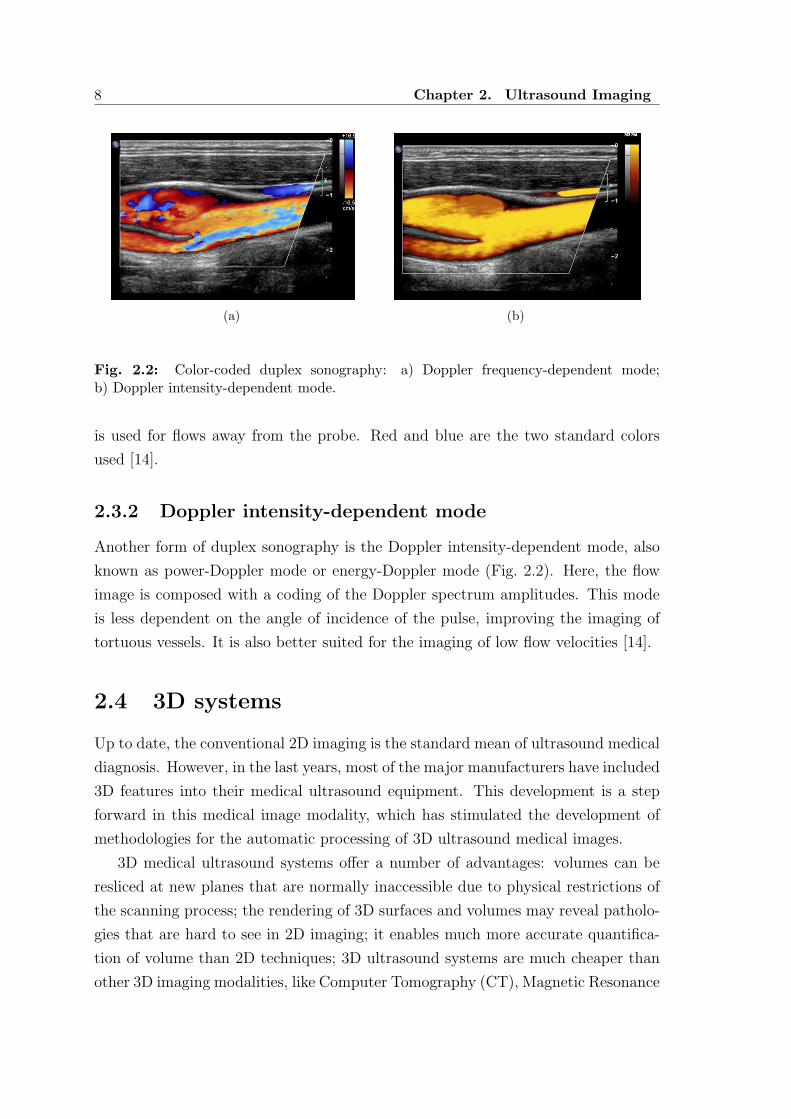
(a) (b)
Fig. 2.2: Color-coded duplex sonography: a) Doppler frequency-dependent mode;b) Doppler intensity-dependent mode.
is used for flows away from the probe. Red and blue are the two standard colors
used [14].
2.3.2 Doppler intensity-dependent mode
Another form of duplex sonography is the Doppler intensity-dependent mode, also
known as power-Doppler mode or energy-Doppler mode (Fig. 2.2). Here, the flow
image is composed with a coding of the Doppler spectrum amplitudes. This mode
is less dependent on the angle of incidence of the pulse, improving the imaging of
tortuous vessels. It is also better suited for the imaging of low flow velocities [14].
2.4 3D systems
Up to date, the conventional 2D imaging is the standard mean of ultrasound medical
diagnosis. However, in the last years, most of the major manufacturers have included
3D features into their medical ultrasound equipment. This development is a step
forward in this medical image modality, which has stimulated the development of
methodologies for the automatic processing of 3D ultrasound medical images.
3D medical ultrasound systems offer a number of advantages: volumes can be
resliced at new planes that are normally inaccessible due to physical restrictions of
the scanning process; the rendering of 3D surfaces and volumes may reveal patholo-
gies that are hard to see in 2D imaging; it enables much more accurate quantifica-
tion of volume than 2D techniques; 3D ultrasound systems are much cheaper than
other 3D imaging modalities, like Computer Tomography (CT), Magnetic Resonance

2.4. 3D systems 9
Imaging (MRI) or Positron Emission Tomography (PET); it is not ionizing nor in-
vasive and the risk to the patient is very small; and it allows better documentation
of the examination [12].
The 3D ultrasound imaging has been applied to a number of medical areas, some
of which are: cardiology; obstetrics; prostate volumes; detection of atherosclerosis
in the carotid artery; breast masses; liver tissues; kidney tissues [12,16].
Despite its advantages, 3D ultrasound diagnosis is not yet a common technique
in routine clinical practice. There are some issues that have to be further improved,
in particular: the inability to acquire large volumes; the sensitivity of the 3D sensors
to metallic objects; long processing times; and demanding protocols for scanning.
Nevertheless, it is believed that this picture will change in the near future [12].
2.4.1 Current techniques
In 3D ultrasound systems, image volumes are usually acquired by sweeping a conven-
tional 2D probe over the area of interest and tracking the position and orientation
of the resulting B-scans. Acquisition systems can be grouped according to: a) the
way they determine the position of the B-scan; b) the restrictions imposed to the
motion of the probe. Commercialized 3D scanning protocols can be of the following
type: linear drawback; rotational; fan; linear; volume; freehand. A short description
of their characteristics and typical applications can be found in [12].
2.4.2 The freehand 3D system
The most popular protocol is the 3D freehand system (Fig. 2.3) because it is the
cheapest and the most flexible, since the probe is moved by hand in an arbitrary
manner. Its main drawbacks are the difficulty to avoid motion artifacts and the
need to attach a position sensor to the probe. Motion artifacts can be caused
by movements of the patient (e.g., respiration or cardiac pulses) or an irregular
pressure of the probe during the manual sweeping. The attachment of an external
position sensor to the probe is not desirable because it disturbs the clinical routine.
Moreover, most position sensors are magnetic devices that are sensitive to metallic
objects. However, some manufactures are now beginning to commercialize new
freehand probes with integrated 3D sensors.
An important issue is whether to work with voxels (3D equivalent of pixels) or
directly with the non-regularly spaced data obtained with the 3D freehand system.
There are many mature tools for displaying and analyzing voxel arrays [12], but this

10 Chapter 2. Ultrasound Imaging
Fig. 2.3: 3D freehand ultrasound system.
approach has several problems: the B-scans have to be resampled onto a regular
voxel array before any further processing; slices obtained from interpolated voxel
arrays are rarely as good as the original B-scans; high resolution voxel arrays requires
large storage space in memory; B-scans are more familiar to experts, facilitating the
detection of boundaries between different tissues. The main disadvantage of working
directly with the irregularly spaced data is the heavier computational effort that its
processing demands.
2.5 Ultrasound imaging of the carotid
2.5.1 Atherosclerosis
Atherosclerosis is an inflammatory disease of blood vessels caused by the accumu-
lation of lipoproteins in artery walls. This deposit of lipids is known as plaque
(Fig.2.4) and may include calcified tissues [18].
The formation of plaque causes a stenosis (narrowing) of the artery, reducing
the blood supply to the organ it feeds. If a piece of the plaque is released, it may
cause the formation of a thrombus that will rapidly slow or stop the blood flow,
leading to an infarction, the death of the tissues fed by the artery. Two well known
types of infarction are: the myocardial infarction (heart attack); and the stroke,
a cerebrovascular accident (CVA) that results in the loss of brain functions [1, 2].
These cardiovascular accidents are frequently fatal and for those who survive the
therapeutic options are limited. Early diagnosis and treatment is crucial to prevent
more serious stages of the disease [18].
The intima-media thickness (IMT) of extracranial carotid arteries is an index
of individual atherosclerosis and is used in clinical practice for cardiovascular risk
2.5. Ultrasound imaging of the carotid 11
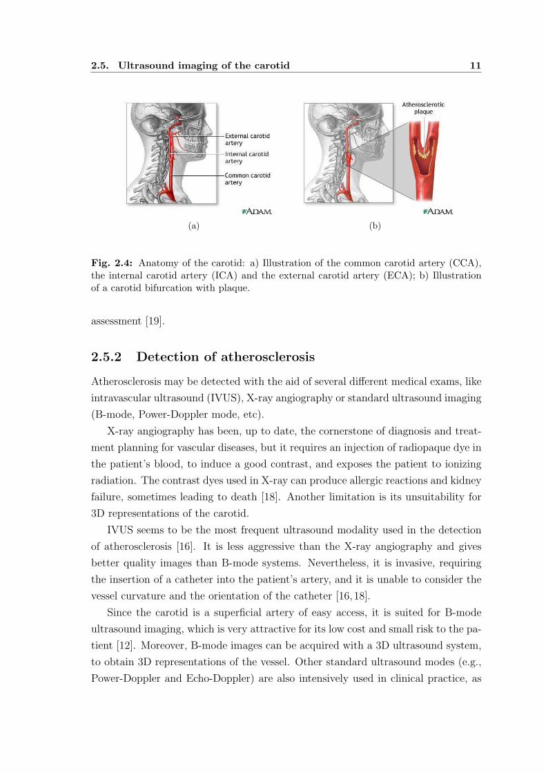
(a) (b)
Fig. 2.4: Anatomy of the carotid: a) Illustration of the common carotid artery (CCA),the internal carotid artery (ICA) and the external carotid artery (ECA); b) Illustrationof a carotid bifurcation with plaque.
assessment [19].
2.5.2 Detection of atherosclerosis
Atherosclerosis may be detected with the aid of several different medical exams, like
intravascular ultrasound (IVUS), X-ray angiography or standard ultrasound imaging
(B-mode, Power-Doppler mode, etc).
X-ray angiography has been, up to date, the cornerstone of diagnosis and treat-
ment planning for vascular diseases, but it requires an injection of radiopaque dye in
the patient’s blood, to induce a good contrast, and exposes the patient to ionizing
radiation. The contrast dyes used in X-ray can produce allergic reactions and kidney
failure, sometimes leading to death [18]. Another limitation is its unsuitability for
3D representations of the carotid.
IVUS seems to be the most frequent ultrasound modality used in the detection
of atherosclerosis [16]. It is less aggressive than the X-ray angiography and gives
better quality images than B-mode systems. Nevertheless, it is invasive, requiring
the insertion of a catheter into the patient’s artery, and it is unable to consider the
vessel curvature and the orientation of the catheter [16,18].
Since the carotid is a superficial artery of easy access, it is suited for B-mode
ultrasound imaging, which is very attractive for its low cost and small risk to the pa-
tient [12]. Moreover, B-mode images can be acquired with a 3D ultrasound system,
to obtain 3D representations of the vessel. Other standard ultrasound modes (e.g.,
Power-Doppler and Echo-Doppler) are also intensively used in clinical practice, as

12 Chapter 2. Ultrasound Imaging
complements to B-mode imaging. However, B-mode images give the best picture of
the anatomical structure of the scanned tissues. Therefore, they are the best option
for automatic segmentation of the carotid tissues.
In ultrasound images, the carotid wall is characterized by echogenic lines sep-
arated by a hypoechogenic space, an intensity valley shaped edge known as the
’double line’ pattern. In longitudinal sections of the carotid, the artery wall ap-
pears as smooth open contours that extend from one image side to the other. In
transversal sections the wall contour has an ellipsoidal shape. The carotid lumen ap-
pears as a dark region, sometimes speckled with brighter granularities due to noise.
The plaque, when present, is localized between the artery wall and the lumen, has
variable response to the echo and frequently shows a texture similar to the tissues
surrounding the artery.
The bifurcation of the carotid (Fig.2.4) and the internal carotid artery (ICA)
are more prone to atherosclerosis, due to stronger hemodynamic stresses in the
bifurcation and branching zones. Unfortunately, it is difficult to visualize the ’double
line’ pattern at these locations. For these reasons, the common carotid artery (CCA)
has received special focus of IMT measurements in B-mode ultrasound imaging
[20], not only in the clinical practice but also in the development of segmentation
algorithms, by the image processing community.

Chapter 3
STATE OF THE ART
Automatic segmentation methods have been intensively applied to a wide variety of
medical imaging modalities, like X-ray, magnetic resonance imaging (MRI), X-ray
computed tomography (CT) and ultrasound.
The ultrasound modality presents a huge challenge to automatic segmentation
due to its very poor quality, when compared with other medical imaging modalities.
Ultrasound images are characterized by [12,16,18]: strong speckle noise, non-uniform
echo intensity, low contrast, movement artifacts, gaps in organ boundaries due echo
dropouts and shadows. These difficulties are behind the minor attention given to
ultrasound diagnosis, when compared to other image modalities. However, in the last
years there has been a large increase in the interest in medical ultrasound imaging,
as a result of advances in its quality and resolution, allied to several advantages
relative to other modalities, like its portability, its non-invasive nature and safety
for the patient, not to mention the fact that it is a much cheaper modality. This
fact is well illustrated in [16], a very recent and comprehensive survey of the state of
the art in the field of ultrasound image segmentation, and in the interesting paper
of Gee et al. [12] about freehand 3D ultrasound systems.
As demonstrated in [16], unlike what happens in other imaging modalities, gen-
eral methods of image segmentation usually fail in ultrasound images. It seems
that the segmentation approaches that try to model the image physics have been
more successful. This survey also shows that most of the effort has been focused
on the segmentation of echocardiography, breast ultrasound, transrectal ultrasound
(TRUS), intravascular ultrasound (IVUS), and ultrasound imaging in obstetrics and
gynecology. On the other hand, the number of published works on 2D segmenta-
tion is far more extensive than 3D approaches, which are taking their first steps.
The authors also make some pertinent observations about the validation in this
field, namely: a) the manual delineation on clinical images is by far the most pop-
ular means of performance assessment, although it generally introduces inter- and

14 Chapter 3. State of the art
intra-expert variability; b) there is no standardization of performance measures,
which hinders the direct comparison of different methods; c) there are no standard
databases on which different groups can compare methods; d) many of the papers do
not validate their results on a database and those who do it frequently use databases
with less than 50 cases.
Concerning the methodology used, ultrasound segmentation algorithms may be
grouped according to the considered specific constraints, in particular, the way
speckle noise is dealt with, the used shape priors and the chosen image features,
like the echo intensity, its gradient and texture measures. In most cases, a combina-
tion of several of these constraints gives better results. The choice of which to use
is application specific.
Whether the segmentation is done in 2D or in 3D, level set active contours
[21–23], also known as geometric snakes, have become the dominant tool in medical
imaging, due to its many advantages, like the easy integration of regional statis-
tics, the topological preservation and their powerful ability to accurately detect
anatomical boundaries and surfaces with arbitrary shapes. This fact can be con-
firmed in [24], a very interesting survey and comparative analysis of parametric and
geometric snakes applied to medical image processing. However, their success in
ultrasound images usually depends on the ability to incorporate some shape prior
restriction into the evolution of the active contour. Otherwise, the snake will often
leak through gaps in the boundaries of the tissues.
This review will focus on the work done on the segmentation of ultrasound images
of the carotid. For a wider and detailed perspective of the methodologies used in
other fields of ultrasound image segmentation we suggest Noble’s survey [16].
There are a number of very interesting examples of shape-based segmentation
[25–39], most of which have been applied with success to ultrasound images. Shape
priors are very popular in ultrasound images because large parts of the data are
often missing or corrupted by strong noise. But, as pointed out in [16], the appli-
cation of shape constraints to disease cases (like carotids with plaque) is still an
open issue. In the particular case of the carotid artery, we may also be faced with
the large variability of the shape, which depends not only on its deformation due
to pressure but also on the position and orientation of the acquired slices. In fact,
unlike most other applications where the whole organ is imaged, different B-scans
of the carotid may correspond to different parts of the artery, with quite different
anatomy. In the segmentation of 3D volumes, the shape variability may become
simpler. But this is a serious and discouraging problem if the vessel boundaries

15
are segmented frame by frame. Things get worse if the B-scans are acquired with
arbitrary orientation. However, this is not the case in clinical practice, where the
B-scans are always approximately normal or parallel to the major axis of the artery.
These orientations give the best picture of the vascular structure. In fact, these ori-
entations are also convenient when acquiring sequences of frames with 3D freehand
systems, to minimize the losses in the visibility of the boundaries between different
tissues.
Speckle noise is inherent to ultrasound imaging and appears in the form of a
granular texture of the echogenic regions. This texture appearance does not cor-
respond to underlying tissue structure but the speckle intensity depends on the
scanned tissue [16]. Therefore, it may be used to improve the segmentation. It
is also frequently viewed as just noise to be reduced. The acquisition process of
ultrasound images starts with a coherent summation of the echo signals produced
by tissue scatterers. The density and spatial distribution of the scatterers depend
on the scanned tissues and determine the statistical distribution of the speckle.
Several statistical distributions (e.g., Rayleigh distribution [40, 41], Rice distribu-
tion [40, 42], K-distribution [43, 44], generalized K-distribution [44, 45] and homo-
dyned K-distribution [44,45]) have been proposed in literature to model the speckle
noise under several scattering conditions. Most of these models are very complex to
analyze and are applicable only to non-compressed signals. However, log-compressed
ultrasound images are the most common in clinical practice, due to their reduced
intensity dynamic range. Statistics of the log-compressed ultrasound signals have
also been proposed [46, 47]. Extensive work has been published on speckle reduc-
tion (most of which use wavelets [48–50] and anisotropic diffusion [51–54]) and tissue
characterization from speckle [15,42,43,55–61]. Speckle does not seem to bring much
information to the segmentation of the carotid artery in B-mode images. Therefore,
in this case, it is usually viewed as just noise.
Texture measures may give good discriminating features and have been used
with success in the classification of several tissues in clinical ultrasound images,
such as breast masses, liver tissues, kidney tissues and the prostate tissues [16].
There has also been some success in the classification of different kinds of carotid
plaques using texture measures [62, 63]. But texture based segmentation is much
more difficult and may not be possible for B-mode images of the carotid. The degree
of discrimination in carotid plaques is very low and large regions of interest have to
be considered in the extraction of their features. There is also strong evidence [64]
that echogenic plaques and the tissues surrounding the artery have, in general, very
16 Chapter 3. State of the art
similar texture properties. On the other hand, hypoechogenic plaques can easily be
misclassified as part of the lumen region. In fact, we may find some weak speckle
noise inside the lumen that is stronger than the echo produced by hypoechogenic
plaques. Our experiments with banks of Gabor filters [65, 66] confirmed the strong
similarity between echogenic regions of interest.
The echo intensity gradient is the most frequent edge detector [67] in general
image segmentation. But it was conceived for images affected by additive noise.
Therefore, in spite of its popularity in ultrasound image segmentation, it is not well
suited for ultrasound images, where the noise has a multiplicative nature. A better
edge detector, known as the instantaneous coefficient of variation (ICOV) [51, 52],
has been specifically conceived for these images. The echo intensity along with its
gradient are the most frequently used features in the segmentation of B-mode images
of the carotid.
3.1 Segmentation of the carotid in 2D B-mode
images
In the particular case of the ultrasound diagnosis of atherosclerosis, IVUS seems to
be the most frequent modality [16]. It is less aggressive than the X-ray angiography
and gives better quality images than freehand B-mode systems. Nevertheless, it is
still invasive, requiring the insertion of a catheter into the patient’s artery, and it is
unable to consider the vessel curvature and the orientation of the catheter [16,18].
In spite of the attractive advantages of freehand B-mode imaging of the carotid,
there isn’t much literature on its automatic segmentation, probably due to the ex-
treme difficulty in the automatic detection of the carotid boundaries in these images.
In fact, although Noble’s survey [16] is very recent and comprehensive, it dedicates
only five lines to this particular problem.
In the first published attempts to detect the carotid boundaries in ultrasound
images [3–5], a previous manual segmentation of the boundary was needed. The
location of the boundary was then refined, according to the local value of a single
image feature, like the echo intensity or the intensity gradient. These approaches
suffered from two important weaknesses: first, the large manual intervention needed,
which is time consuming and prone to subjective segmentation results; second, the
utilization of a single image feature is usually not enough to correctly detect the
carotid boundaries in B-mode images, characterized by strong speckle noise, echo

3.1. Segmentation of the carotid in 2D B-mode images 17
dropouts and large discontinuities in the boundaries.
More powerful approaches were proposed in [6, 7]. A common characteristic
of these approaches is the minimization of a global cost function through dynamic
programming (DP). The cost function may integrate multiple image features, like the
echo intensity and its gradient, and a local geometric constraint to guide and smooth
the estimated contour. Each feature or constraint is represented by a cost term and
the relative importance of each term is determined by a weighting factor previously
determined in a training stage. These models produce more robust segmentations
with less human intervention, specially in the case of [6]. In a later study [68], the
DP algorithm proposed in [6] also demonstrated better performance when compared
with some alternative approaches, like the maximum gradient algorithm [5] and the
matched filter algorithm [69].
More recently, an improvement of [6] was proposed in [8]. The main novelties
are the embedding of the DP algorithm in a multiscale scheme, to get a first rough
estimate of the carotid wall boundaries, and the incorporation of an external force
as a new term in the cost function, which allows the human intervention over the
selected best path, in case of incorrect detection. This model was tested against a
large data set with promising results and has the advantage of being relatively fast.
But it has several important drawbacks: its performance is significantly affected by
the presence of plaque and other boundaries; frequently, human correction is also
needed when the quality of the images is poorer; the determination of the optimal
weight vector requires an exhaustive search in the weight space and a different
vector has to be computed for each boundary; a retraining of the system may have
to be done for images acquired with different ultrasonic equipment, although the
authors reported consistent results, without retraining, for an image set taken with
a different scanner; DP implementations are not suited for the incorporation of
global smoothness constraints, which are more powerful than local ones, nor to deal
with deep concavities or sharp saliences that may appear in the boundary of the
plaque; finally, the DP algorithm is not directly applicable to closed contours, which
is possibly the reason why the segmentation of transversal sections of the carotid
was not referred.
Another family of algorithms [9–11] tried to apply parametric snakes [70] to the
detection of the carotid boundaries. Active contours have been used with success
in other fields of medical image segmentation. However, for several reasons, they
do not seem to be the best choice for the segmentation of the carotid wall. First,
they usually require a manual initialization of the snake in the close vicinity of the

18 Chapter 3. State of the art
carotid boundaries. This implies intensive human intervention and the algorithms
appear more like methods for refinement of the boundary location and less like
automatic segmentation algorithms. Second, the propagation force is frequently
based on intensity gradients and, therefore, they tend to be very vulnerable to the
attraction by false edges, located between the initialized snake and the boundary to
be detected. Third, these snakes usually leak at wall gaps where there is no gradient
or it is too weak.
In [9], the leaking problem was solved by discarding all images with big boundary
gaps. They also excluded the images where the lumen boundary or the carotid wall
boundary could not be defined visually. The snake has to be initialized manually
and very close to the far end lumen boundary or the far end wall boundary, the
only boundaries detected in this work. The intensity gradient was the only image
feature considered in the energy of the snake. Some statistics computed for a large
data base of longitudinal sections showed a smaller variability than manual tracings
done by experts.
A more sophisticated external force was used in [10, 11], but also based on the
intensity gradient, which means the snake is still sensitive to local noise and bound-
ary gaps. Once again, the segmentation was done only for the far end boundaries of
the carotid, in longitudinal sections. The user just has to specify the starting and
the end points of the snake, significantly reducing the human intervention. A small
rectangular region of interest is selected automatically, such that the former two
points are included in this region. Then, for each vertical line inside this region, the
first edge found in the downward direction is taken as a pixel of the lumen boundary.
From this initial contour, the snake finds the final location of the lumen boundary.
To detect the wall boundary, the snake is displaced downwards about 0.05 cm and a
new search is done for the global minimum of the snake’s energy. Some results were
presented but the work lacks a validation with statistical meaning.
Quite different approaches were proposed in [71, 72]. In [71], the authors pre-
sented a new scheme for the segmentation of the carotid in B-mode images, based on
the multi-resolution analysis and watershed techniques. In [72], the segmentation
was based on a fuzzy region growing algorithm and thresholding. In both cases,
only the lumen region was segmented and the results were illustrated with a single
image. Both algorithms lack a quantitative validation in clinical images.

3.2. Segmentation of the carotid in 3D B-mode volumes 19
3.2 Segmentation of the carotid in 3D B-mode
volumes
A few works have been published on 3D segmentation of the carotid boundaries from
B-mode volumes. But this topic is still in its beginning and it is usually limited to
the segmentation of the lumen region, leaving out the detection of the wall boundary.
Gill et al. [73] proposed a semi-automatic segmentation of the carotid lumen in
3D ultrasound images, using a dynamic balloon model, which is manually initialized
inside the lumen region. The semi-automatic segmentation obtained for a 3D data
set proved to be close to the fully manual segmentation.
Zahalka and Fenster [74] used a radial search scheme, relative to a seed manually
placed inside the lumen, to get an initial estimate of the lumen boundary. Then, in a
second step, a geometric deformable model (GDM) was applied to obtain a smoothed
final contour. The algorithm was tested in two data sets with good results. However,
the images of these data sets seem to have very low noise in the lumen region and do
not have hypoechogenic plaques. It is not clear how these algorithms would behave
on normal clinical images.
Baillard et al. [75] assumed a normal distribution for the intensity inside the
lumen and a shifted Rayleigh distribution for the intensity in echogenic tissues. The
lumen volume was then segmented with a Stochastic Expectation-Maximization
(SEM) algorithm [76, 77], embedded in a 3D level set scheme. This is a simple
representation of the tissues that does not account for speckle noise inside the lumen
nor large boundary gaps caused by echo dropouts. Moreover, it cannot detect the
wall boundaries and the superposition of the different probability density functions
may give biased estimates of the decision level. The results were only illustrated by
two examples and no quantitative measures were presented in this case.
In [78], the authors reconstructed the carotid wall and the lumen boundary
surfaces from sequences of B-scans acquired with a 3D freehand system. But the
B-scans are manually segmented.
A recent and interesting work can be found in [79,80], where the carotid surfaces
were semi-automatically reconstructed from sequences of B-scans of the artery. Both
the carotid wall and the lumen boundary were segmented, which is a step forward,
when compared to the other referred automatic approaches. However, a gradient
vector flow (GVF) snake [81] was used to detect the carotid boundaries. Therefore,
as other snakes moved under gradient-based forces, the GVF snake may have to
be initialized close to the boundary to be detected, when there are nearby edges

20 Chapter 3. State of the art
originated by noise or from other boundaries. On the other hand, these snakes tend
to leak through boundary gaps, where there is no gradient or it is too weak. Finally,
being a parametric snake, it may need additional processing when a topological
change happens.

Chapter 4
SEGMENTATION OF THE CAROTID
WALL IN B-MODE IMAGES
4.1 Introduction
Automatic segmentation of ultrasound medical images is extremely difficult, due to
their complexity and poor quality. When compared to other applications of med-
ical ultrasound imaging, the segmentation of the carotid artery in B-mode images
presents additional difficulties, like the possible presence of plaque (disease tissue),
which is often difficult to discriminate from other adjacent tissues. In other medi-
cal ultrasound applications, shape-based segmentation is often used with success to
deal with gaps in the boundaries of the examined organ, caused by echo dropouts
and shadows. However, the presence of plaque is an obstacle to the shape-based
segmentation of the carotid. Another obstacle to this segmentation method is the
impossibility to scan the whole organ, which means that different B-scans may corre-
spond to different parts of the artery, with different anatomy. Even in the absence of
plaque, the carotid wall is still very challenging to detect, since it frequently appears
as a diffuse boundary between two echogenic tissues, with large discontinuities.
In spite of several attempts to automatically segment the carotid in B-mode
images, this problem is still far from being well resolved. As a consequence, a
manual segmentation of these images, performed by an experienced medical doctor,
is the usual adopted procedure (see, for instance, [63, 78]), which is a tedious and
time consuming task and tends to give subjective results.
The chapter starts with an overview of the method proposed for the automatic
detection of the carotid wall in B-mode images, followed by several sections where
the algorithm is described in detail, step by step. Finally, several results, computed
from an image data base, and some concluding remarks are presented.

22 Chapter 4. Segmentation of the carotid wall in B-mode images
4.2 Overview of the approach
In face of the difficulties previously described for model-based detection of the
carotid wall in ultrasound images, the ideal segmentation model should not be too
flexible, in order to keep a strong robustness to noise and missing data, nor too rigid
to correctly follow the desired boundary over its whole contour path. Moreover, it
should avoid any gradient based motion, like in snake-based models. These require-
ments suggest looking for the best globally most significant smooth curve, according
to some cost or gain function.
With these requirements in mind, we introduce a new segmentation algorithm
for the detection of the CCA wall in ultrasound images, which looks for the best
smooth curves in the image, according to a new gain function. Our algorithm is
robust to speckle noise, irregular contrast due to echo dropouts and occlusions of
the lumen caused by the plaque. Moreover, it also has the capability of adapting to
flexible tubular shapes.
As in previous works on the segmentation of ultrasound images of the carotid
[6, 8–11, 68], our algorithm was designed for sections of the CCA. But it can also
be used in sections of the internal carotid artery (ICA) or the external carotid
artery (ECA), as long as the image quality is not too poor. As we will show, our
segmentation algorithm can be applied both to transversal and longitudinal sections.
The idea of looking for the most significant path is common to the dynamic pro-
gramming algorithm proposed in [6], but our approach is quite different and presents
several advantages. First, our model includes a global smoothness constraint which
is not easily integrated in the dynamic programming approach. Second, the user
does not have to specify a different region of interest (ROI) for each boundary.
Third, our model does not need a previously determined reference path used as
geometric constraint.
Next we give a global description of our algorithm, leaving most of the details
for further discussion in subsequent sections.
It would be impractical to evaluate all possible paths. So, as an alternative to
look for the best path, we use the very popular random sample consensus (RANSAC)
algorithm [82], which works quite well in practice.
In longitudinal sections, the smooth curve model is a cubic spline with only a
few control points, which has enough stiffness to stay robust to noise but is also
flexible enough to correctly follow the carotid wall along its whole axis, even when
it is severely bended. The locations of the spline control points are dynamically

4.2. Overview of the approach 23
chosen by the algorithm.
In transversal sections, an ellipse is used as the wall model since the wall contour
in these sections has an elliptical shape.
The wall model consensus is measured by a new gain function that integrates
the responses to the most discriminating characteristics of the carotid boundary:
the proximity of the wall model to points of step edges; the proximity to valley edge
points; the consistency between the orientation of the normal to the wall model and
the orientation of the intensity gradient; and the distance to the detected lumen
boundary.
Ideally, the distance to the lumen boundary should be represented by a signed
distance function, here designated by SDL, with negative sign inside the lumen.
It has been shown in [13] that thresholding algorithms may be used to segment
the lumen in B-mode images of the carotid. Nevertheless, this usually produces
more than one dark region, one of which is the lumen region. Moreover, in some
B-mode images of the carotid there may be connections between the lumen region
and other dark regions due to large gaps in the carotid wall. This makes it difficult to
isolate the lumen region from the other dark regions and we end up with the signed
distance to the boundaries of all dark regions. However, if we have an estimate of
the lumen axis position, we may use it to select the surrounding region boundaries
and significantly improve the estimate of the signed distance function.
The proposed algorithm requires a rough location of the lumen axis. This can
easily be computed if we already have an approximate segmentation of the lumen.
Unfortunately, this may not be possible due to the difficulties, discussed above, in
isolating the lumen region. So, in transversal sections, the user has to choose one
single point near the centroid of the lumen. In longitudinal sections, the user has
to choose between 2 and 4 points roughly near the lumen medial axis, depending
on the curvature of the carotid wall. If the carotid has low curvature along the
medial axis, one point at each extremity will be enough. Nevertheless, this is faster
and easier than selecting the whole ROI or initializing a snake close to the carotid
boundary we want to detect.
We also introduce a new robust non-linear image filter, suited to ultrasound im-
ages, to compute an edge map with reduced noise and good localization of the edges.
Our filter combines the properties of Tauber’s anisotropic diffusion filter [53], which
is well suited to ultrasound images in general, with a curvature dependent diffu-
sion property that improves the preservation of objects with low curvature, like the
carotid boundaries. The curvature dependence of the filter borrows concepts from

24 Chapter 4. Segmentation of the carotid wall in B-mode images
Total Variation theory [83, 84] and is incorporated through the Marquina-Osher’s
scheme for a mean curvature motion filter [85]. As in the Tauber’s model, our fil-
ter also incorporates: an edge detector known as the instantaneous coefficient of
variation (ICOV) [51, 52], more suited to the multiplicative nature of the speckle
noise; the Tukey’s function as the ’edge stopping’ function, to improve the auto-
matic stopping of the diffusion and produce sharper boundaries; and the median
absolute deviation (MAD) as a base for the edge scale estimator.
Figure 4.1 shows a block diagram with the main steps of our algorithm, when
applied to longitudinal sections. For transversal sections the procedure is very simi-
lar, except that instead of splines we have ellipses, instead of the lumen medial axis
we have the lumen centroid and, finally, the dominant gradient direction block is not
used. The input is an ultrasound image of the CCA, from which the lumen medial
axis or the lumen centroid is obtained. The lumen medial axis is used to automati-
cally select a ROI from the image and to improve the estimate of the signed distance
to the lumen boundary. This signed distance computation also relies on a binary
image computed from the ROI through a thresholding algorithm. The non-linear
image filter is applied to the ROI to get a smooth image for which a gradient map
and an edge map are computed. The spline model depends on the gradient orien-
tation at the control points. So, the gradient map is substituted by the map of the
local dominant gradient direction, with reduced error in the gradient orientation.
The edge map is cleaned of all edges incompatible with the carotid walls and then
used, in conjunction with the ROI and the dominant gradient map, to compute the
valley edge map. Finally, the cleaned edge map, the valley edge map, the dominant
gradient map and the signed distance to the lumen boundary are used as inputs to
the gain function, during the RANSAC search. The outputs are the best splines
found, above and bellow the lumen axis, according to the specified gain function.
The wall model can be further improved, in a subsequent step, through a function
minimization in the vicinity of the solution found by the RANSAC search.
4.3 Lumen axis and ROI selection
The whole procedure starts with the user pointing out the approximate location of
the lumen axis. This is done by clicking over the image with the mouse.
In transversal sections, only one click is necessary, near the centroid of the lumen.
In longitudinal sections, the user has to enter at least one point at each extremity of
the longitudinal axis. If the axis is significantly bended, then one or two additional

4.4. Determination of the SDL 25
Fig. 4.1: Block diagram with the main steps of the proposed algorithm.
points should be entered along the lumen axis. This is the only human interaction
needed. If the user enters more than one point, the algorithm assumes the image is
a longitudinal section and completes the medial axis by cubic spline interpolation.
Figure 4.2 illustrates the procedure for two sections of the CCA.
In the segmentation of 3D volumes, formed by sequences of B-scans, the user
intervention is only required in the first frame. For the other frames, the estimation
of the lumen axis location is done automatically, inferring this information from the
segmentation of the previous frame.
Once the approximate location of the lumen axis is known, the ROI is selected,
as shown in Fig. 4.2 (b) and Fig. 4.2 (d). Assuming the artery boundaries will not be
at a distance, d, from the lumen axis, larger than a certain threshold, dmax, the ROI
may be chosen as the smallest rectangular box containing all image pixels within
distance dmax to the lumen axis. This distance threshold can be estimated from the
largest carotid found in an image data base. By limiting the image processing to
this ROI, the computational effort is reduced.
4.4 Determination of the SDL
The signed distance to the lumen boundary is determined over the selected ROI
box.
As will be demonstrated in chapter 5, the triangle thresholding algorithm [86] is
a quick way to compute a good rough estimate of the lumen region. Therefore, it

26 Chapter 4. Segmentation of the carotid wall in B-mode images
(a) (b)
(c) (d)
Fig. 4.2: Localization of the lumen axis by the user: a) A longitudinal section of theCCA; b) The ROI box (in red) for the longitudinal section, the interpolated lumen medialaxis (green curve) and the four points entered by the user, represented as large green dotsover the axis curve; c) A transversal section of the CCA; d) The ROI box (in red) forthe transversal section and the single point entered by the user, represented a large greencross inside the lumen region.

4.5. Non-linear image filtering 27
(a) (b)
(c) (d)
Fig. 4.3: Determination of the SDL in a longitudinal section: a) Binary image computedfrom the ROI box; b) Estimated lumen region; c) Boundary of the estimated lumen region;d) |SDL| represented as an intensity map.
is used to estimate an intensity threshold, with which a binary version of the ROI
is computed. The binary images obtained for the ROI’s of Fig. 4.2 (b) and (d) are
shown in Fig. 4.3 (a) and Fig. 4.4 (a), respectively.
Using the lumen axis specified by the user as a reference, an estimate of the
lumen region is computed as the set of black pixels in the binary image that can be
reached from the lumen axis through a vertical line, in longitudinal sections, or a
radial Bresenham line [87], in transversal sections. This procedure is illustrated in
Fig. 4.3 (b) and Fig. 4.4 (b).
Figure. 4.3 (c) and Fig. 4.4 (c) show the boundary pixels of the estimated lumen
region, determined as the set of pixels of the lumen region that have at least one
4-neighbor outside the lumen.
Finally, the Euclidean distance map to the lumen boundary is computed with
the second algorithm described in [88], setting to negative the distances inside the
lumen region. Figure 4.3 (d) and Fig. 4.4 (d) show the intensity maps of |SDL|,for the longitudinal section and the transversal section, respectively. Here, larger
absolute distances were represented by brighter intensities.
4.5 Non-linear image filtering
To get the edge map from the ultrasound image, a smooth version of the original
image is first computed, using low-pass filtering. Then, an edge detector is applied
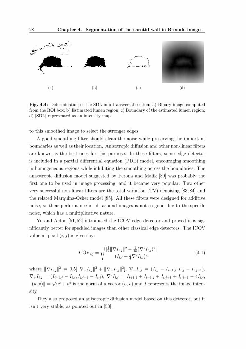
28 Chapter 4. Segmentation of the carotid wall in B-mode images
(a) (b) (c) (d)
Fig. 4.4: Determination of the SDL in a transversal section: a) Binary image computedfrom the ROI box; b) Estimated lumen region; c) Boundary of the estimated lumen region;d) |SDL| represented as an intensity map.
to this smoothed image to select the stronger edges.
A good smoothing filter should clean the noise while preserving the important
boundaries as well as their location. Anisotropic diffusion and other non-linear filters
are known as the best ones for this purpose. In these filters, some edge detector
is included in a partial differential equation (PDE) model, encouraging smoothing
in homogeneous regions while inhibiting the smoothing across the boundaries. The
anisotropic diffusion model suggested by Perona and Malik [89] was probably the
first one to be used in image processing, and it became very popular. Two other
very successful non-linear filters are the total variation (TV) denoising [83, 84] and
the related Marquina-Osher model [85]. All these filters were designed for additive
noise, so their performance in ultrasound images is not so good due to the speckle
noise, which has a multiplicative nature.
Yu and Acton [51, 52] introduced the ICOV edge detector and proved it is sig-
nificantly better for speckled images than other classical edge detectors. The ICOV
value at pixel (i, j) is given by:
ICOVi,j =
√
|12‖∇Ii,j‖2 − 1
16(∇2Ii,j)2|
(Ii,j + 14∇2Ii,j)2
(4.1)
where ‖∇Ii,j‖2 = 0.5[‖∇−Ii,j‖2 + ‖∇+Ii,j‖2], ∇−Ii,j = (Ii,j − Ii−1,j, Ii,j − Ii,j−1),
∇+Ii,j = (Ii+1,j − Ii,j, Ii,j+1 − Ii,j), ∇2Ii,j = Ii+1,j + Ii−1,j + Ii,j+1 + Ii,j−1 − 4Ii,j,
‖(u, v)‖ =√u2 + v2 is the norm of a vector (u, v) and I represents the image inten-
sity.
They also proposed an anisotropic diffusion model based on this detector, but it
isn’t very stable, as pointed out in [53].

4.5. Non-linear image filtering 29
To decide which edges are boundaries, we need an estimate of the image edge
scale, σe. We expect that most of the image pixels belong to homogeneous regions,
with low ICOV values. Boundaries will be outliers, with large ICOV values. As
in [53,90], we appeal to tools of robust statistics to estimate σe, by computing a scale
of the image ICOV based on its median absolute deviation (MAD). In particular,
we use the measure proposed in [53], which is better formulated than in [90] and is
given by
σe = CMADΩ
(ICOV) + medΩ
(ICOV)
= CmedΩ
|ICOV − medΩ
(ICOV)| + medΩ
(ICOV)(4.2)
where medΩ
(r) is the median of r over the image domain, Ω, and C = 1.4826 is a
constant, derived from the fact that the MAD of a zero-mean normal distribution
with unit variance is 1/1.4826. The measure proposed in [90] is not correct because
it uses just the first term of equation 4.2. Therefore, it measures the deviation of
the data sample relative to its median, which cannot be directly compared with the
data of the sample [53].
In [90], Black and his colleagues showed that the anisotropic diffusion is the gra-
dient descent of an estimation problem with a particular robust error norm taken
from the robust statistic field, which deals with problems where the data has large
errors or outliers. They also showed that diffusion with Tukey’s norm function
produces sharper boundaries than the diffusion with the Lorentzian norm (corre-
sponding to the Perona-Malik model [89]) and the L1 norm (which is equivalent to
the TV formulation of Rudin and Osher [83, 84]). Tauber [53] used these results to
propose a new anisotropic diffusion model for ultrasound images:
∂I(x,y;t)∂t
= div [c(x, y; t)∇I(x, y; t)]I(x, y; 0) = I0(x, y)
∂I(x,y;t)∂−→n
= 0 ∀(x,y)∈∂Ω
(4.3)
where t is the time, div represents the divergence, ∇I is the intensity gradient, I0 is
the initial image, at time t = 0, ∂Ω is the image boundary, −→n is the outward normal
at the image boundary and c(x, y; t) is the diffusion coefficient, here computed as

30 Chapter 4. Segmentation of the carotid wall in B-mode images
the value of the Tukey’s function for a pixel (x, y), at time t, and given by
c(x, y; t) =
12
[
1 −(
ICOV(x,y;t)σs(t)
)2]2
ICOV < σs
0 ICOV ≥ σs
(4.4)
The model described by equation 4.3 uses the Tukey’s error norm [90] as the
’edge stopping’ function and the ICOV edge detector. One must set σs =√
5σe
in order to obtain forward diffusion when ICOV < σe and edge enhancement when
ICOV > σe [53, 90].
In ultrasound images, the Tauber’s filter offers significant improvement, when
compared to other models, in the detection of boundaries of objects. This is a
direct consequence of using the ICOV edge detector, well adapted to multiplicative
noise, and robust statistics to decide where the diffusion should take place and where
it should be inhibited. Nevertheless, it has the inconvenience of destroying some
important anatomical boundaries when they have low contrast at bright regions,
where the ICOV is weak. An example of this problem can be seen in Fig. 4.5 (b),
where the Tauber’s model destroyed the weak valley edge pointed by the arrow inside
the circle. To overcome this problem, we borrow concepts from the TV theory [83,84]
and introduce the following model
∂I(x,y;t)∂t
= c(x, y; t)κ(x, y; t)‖∇I(x, y; t)‖I(x, y; 0) = I0(x, y)
∂I(x,y;t)∂−→n
= 0 ∀(x,y)∈∂Ω
(4.5)
where c(x, y; t) is the Tukey’s function given by equation 4.4 and κ(x, y) is the mean
curvature, updated at each time step and given by
κ(x, y) = div
( ∇I(x, y)‖∇I(x, y)‖
)
(4.6)
Equation 4.5 includes the curvature information and keeps the important prop-
erties of Tauber’s filter. It can be seen as a curvature flow with the Tauber’s tensor
placed as a spatially varying parameter. As in the Tauber’s model, the diffusion
is inhibited or completely stopped at places where the ICOV is high. But it also
inhibits diffusion where the curvature is small, as is usually expected for anatomical
structures. On the other hand, the noise is strongly smoothed out because it usually
has high curvature and low ICOV. As can be seen in Fig. 4.5 (c), our filter not only

4.6. Edge map 31
(a) (b) (c)
Fig. 4.5: Edge maps produced by non-linear image filtering: a) Part of a longitudinalsection of a CCA, with a weak valley edge pointed by an arrow; b) The edge map producedby the Tauber’s anisotropic filter shows a completely destroyed valley edge inside themarking circle and some degradation of its position outside the circle; c) The edge mapproduced by our filter shows a better preservation and localization of the weak valley edge.
produces well localized edges but it is also able to preserve important anatomical
boundaries that are destroyed by the Tauber’s filter.
We used a similar numerical scheme to the one found in [53] for the PDE in
equation 4.3 and the numerical scheme proposed in [85] for equation 4.5.
4.6 Edge map
Once we have a smooth image, obtained with the proposed non-linear image filter,
we need to select the stronger edges. We use the non-maxima suppression with
hysteresis algorithm, a popular scheme introduced in [67] that works well. How-
ever, in our case, the gradient norm is replaced by the ICOV. In other words,
instead of using ‖∇I‖(cos(θ), sin(θ)), where θ is the gradient orientation, we use
ICOV (cos(θ), sin(θ)), thus replacing the gradient norm by the ICOV for the edge
strength, but keeping the gradient orientation information. In the non-maxima sup-
pression, the edge map will be the set of pixels that are local maxima of the ICOV
in the direction of the gradient and have ICOV value above a specified threshold, T1.
The hysteresis consists in keeping also weaker edges that are local maxima as long as
they have an ICOV value above a second threshold, T2 < T1, and are connected to
the stronger edges by some path of edge pixels. We use equation 4.2 to compute σe
for the final smooth image and set T1 = σe. A good range for the second threshold

32 Chapter 4. Segmentation of the carotid wall in B-mode images
is T1/3 < T2 < T1/2 [67]. Therefore, we set T2 = 0.4T1. Finally, the edge map
is processed by the morphological thinning algorithm introduced in [91], which is
known to produce good results.
4.6.1 Dominant gradient direction
An additional step that became necessary at this stage, for the subsequent spline
fitting in longitudinal sections of the carotid, was the reduction of the gradient
orientation errors. This error reduction may be achieved through the computation
of the local dominant gradient direction, at each image pixel. This step will not be
necessary for transversal sections, but all other edge map operations, described in
the next subsections, are common to both longitudinal and transversal sections of
the carotid.
The dominant gradient direction is computed with an iterative procedure. Let
∇Ini,j be the intensity gradient for pixel (i, j), at iteration n, and ∇In−1
k the gradient
for the kth pixel in the 8-neighborhood of (i, j), at iteration n−1. We compute ∇Ini,j
as the average of ∇In−1k , for k = 1, 2, ..., 9:
∇Ini,j =
1
9
9∑
k=1
∇In−1k (4.7)
To avoid the interference of close contours with very different orientation (e.g.,
as in valley shaped edges), gradients with opposite direction to the gradient of the
central pixel should not be included in the gradient average. We consider that two
vectors have opposite direction if their inner product is negative, which is equivalent
to an angle larger than 90 between them. Let βk be the angle between the gradient
of the central pixel, (i, j), and the gradient of each of its 8 neighbors. Then, βk
should be less than 45 in order to guarantee a positive inner product for all pairs
of gradients used in equation 4.7.
We expect that pixels in homogeneous regions will have no local dominant direc-
tion, unless they are close to a region boundary. This will also happen for some of
the detected edge pixels, due to noise. Where there is no local dominant direction,
its value may drift, from iteration to iteration, and may not stabilize. The changes
of the gradient orientation at these pixels may be seen as outliers when compared
to the rest of the population, for which the gradient change becomes smaller at each
iteration. On the other hand, a small fraction of the edge pixels (whose detection
depends on the gradient direction) will disappear and new ones will arise as the gra-
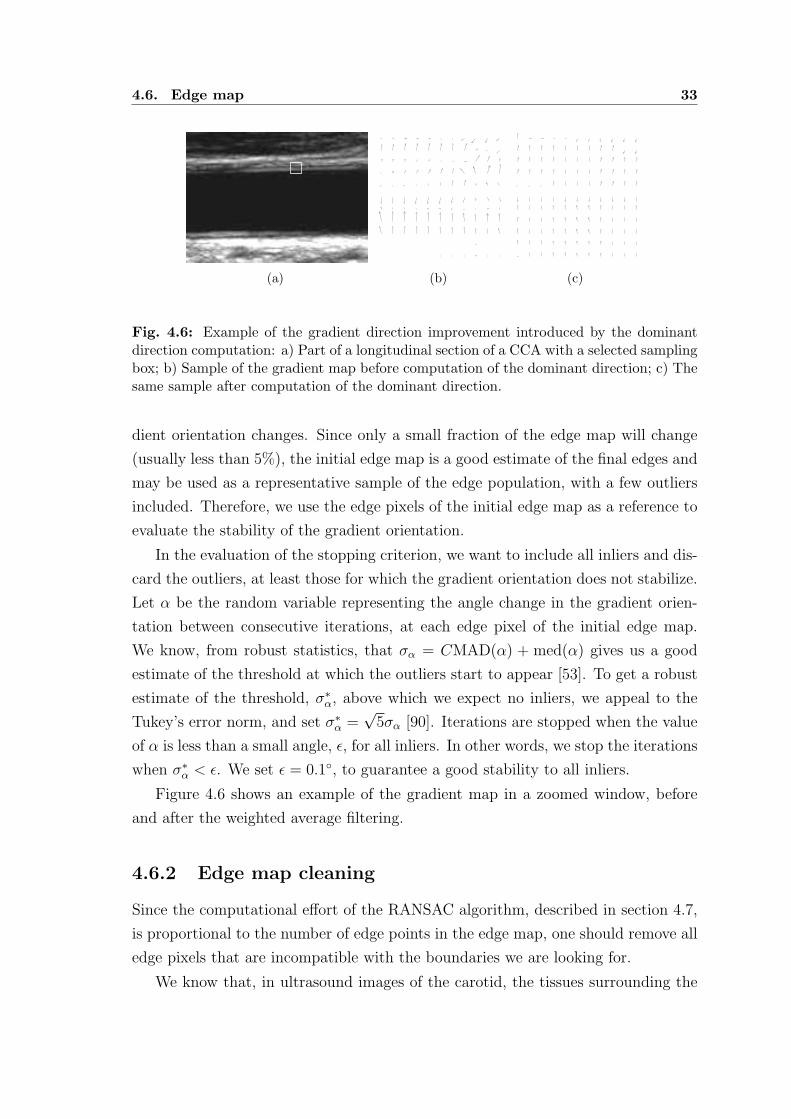
4.6. Edge map 33
(a) (b) (c)
Fig. 4.6: Example of the gradient direction improvement introduced by the dominantdirection computation: a) Part of a longitudinal section of a CCA with a selected samplingbox; b) Sample of the gradient map before computation of the dominant direction; c) Thesame sample after computation of the dominant direction.
dient orientation changes. Since only a small fraction of the edge map will change
(usually less than 5%), the initial edge map is a good estimate of the final edges and
may be used as a representative sample of the edge population, with a few outliers
included. Therefore, we use the edge pixels of the initial edge map as a reference to
evaluate the stability of the gradient orientation.
In the evaluation of the stopping criterion, we want to include all inliers and dis-
card the outliers, at least those for which the gradient orientation does not stabilize.
Let α be the random variable representing the angle change in the gradient orien-
tation between consecutive iterations, at each edge pixel of the initial edge map.
We know, from robust statistics, that σα = CMAD(α) + med(α) gives us a good
estimate of the threshold at which the outliers start to appear [53]. To get a robust
estimate of the threshold, σ∗α, above which we expect no inliers, we appeal to the
Tukey’s error norm, and set σ∗α =
√5σα [90]. Iterations are stopped when the value
of α is less than a small angle, ε, for all inliers. In other words, we stop the iterations
when σ∗α < ε. We set ε = 0.1, to guarantee a good stability to all inliers.
Figure 4.6 shows an example of the gradient map in a zoomed window, before
and after the weighted average filtering.
4.6.2 Edge map cleaning
Since the computational effort of the RANSAC algorithm, described in section 4.7,
is proportional to the number of edge points in the edge map, one should remove all
edge pixels that are incompatible with the boundaries we are looking for.
We know that, in ultrasound images of the carotid, the tissues surrounding the

34 Chapter 4. Segmentation of the carotid wall in B-mode images
artery wall from the outside are brighter than the tissues inside the artery. Therefore,
we should neglect all edges with gradient pointing to the interior of the artery.
This can be easily done if we have a rough estimate of the lumen axis, computed
automatically or specified by the user. Let γ(i, j) be the angle, at a given pixel, (i, j),
between the intensity gradient and the gradient of the distance map to the medial
axis or the lumen centroid. If γmax is the threshold above which the probability of
finding an edge pixel of the carotid wall is virtually zero, then all edge pixels for
which γ(i, j) > γmax may be removed from the edge map.
All edge pixels in the image ROI, described in section 4.3, that have a distance
to the lumen axis larger than a certain threshold, dmax, are also removed from the
edge map.
The ICOV edge detector tends to produce many false edges in dark regions
when the image is very noisy, due to its higher sensitivity at lower intensities. We
may clean many of these false edges using the signed distance map to the lumen
boundary, SDL, described in section 4.4. All pixels with signed distance outside
the range SDLmin < SDL < SDLmax are removed. The determination of these two
thresholds will be discussed in section 4.9.
Figure 4.7 shows an example of the edge map before and after the selection of
the important edges using the above mentioned criteria.
In longitudinal sections, the cleaned edge map is divided into two independent
edge maps, one with the edges above and the other with the edges below the medial
axis, which are separately fed to the RANSAC algorithm. This partitioning is not
done in transversal sections.
4.6.3 Valley edge map
One of the discriminating characteristics of the carotid boundary is its typical in-
tensity profile in the shape of a valley, also called ’double line’ pattern [20]. To use
this information we compute the image valley edge map.
As illustrated in Fig. 4.8 (a), we start by searching, up to a certain distance,
L, the first local intensity maximum in both directions along the line defined by
each edge point, e, and the intensity gradient at that point, ∇I(e). The intensity
profile of a valley edge has two intensity peaks, a and b, being one of these usually
shorter than the other. Due to the strong noise in these images, some step edges
may also have a double peak intensity profile, but their lower peak will be weak.
Therefore, all profiles with only one peak or a weak lower peak should be classified

4.7. Random Sample Consensus (RANSAC) 35
(a) (b)
(c) (d)
Fig. 4.7: Example of the edge map cleaning: a) Longitudinal B-scan of the CCA; b) Es-timated medial axis, ROI box and lumen boundary superimposed on a faded version ofimage (a); c) Complete edge map of the ROI; d) Edge map of the ROI after cleaning.
as step edges. The other intensity profiles, with a strong lower peak, will be valley
edges. To detect the strong lower peaks, we may use an approach similar to the
edge detection scheme described for the edge map, at the beginning of this section.
If we use hysteresis and if A is a random variable representing the amplitude of
the lower peak, we may set the high threshold to TA = CMAD(A) + med(A) and
the low threshold to 0.4TA. However, experimentation showed that using only the
lower threshold is better because it captures more valley edges without a significant
increase in noise. Therefore, in our algorithm, an edge pixel is classified as a valley
edge if A > 0.4TA. As an example, the valley edge map for the ROI of Fig. 4.7 is
presented in Fig. 4.8 (b).
4.7 Random Sample Consensus (RANSAC)
Since the introduction of the RANSAC algorithm [82], a huge amount of work has
been published concerning improvements to the algorithm or its use in different ar-
eas, including computer vision. A brief list of possible applications of the RANSAC
algorithm may be found in [92]. We could not find any application to the segmen-
tation of ultrasound images of the carotid.

36 Chapter 4. Segmentation of the carotid wall in B-mode images
e−L e + Lea b de
I
(a) (b)
Fig. 4.8: Valley edges: a) Illustration of an intensity valley, where: I is the intensity, e isthe location of the edge, de is the distance from the edge in the direction of its intensitygradient, ∇I(e), a is the location of the small peak, b is the location of the large peak,and L is the maximum distance of search; b) Valley edge map for the ROI of Fig. 4.7.
This algorithm deals with the problem of estimating the parameters of a model
from a data set containing a large number of outliers. Its main attraction comes
from the fact that it is simple and works well in practice. It works by repeatedly
extracting from the set of data points a random sample, with the minimum size
required to determine the model parameters. For example, if the model is a straight
line, samples of two points will be drawn, while samples of 5 points are needed if the
model is an ellipse. The consensus of the model, determined for the drawn sample,
is evaluated for the rest of the population. The model with the best consensus is
selected. The number of inliers, defined as the data points closer to the model than
a certain threshold, is the most common criterion for the consensus evaluation. The
process is terminated when there is a high confidence of having drawn at least one
good sample.
One way of estimating the minimum number of samples necessary to get this
confidence is to determine the number of samples that guarantees a low probability
of obtaining only bad samples [93]. Another way is to add a few standard-deviations
to the expected number of samples necessary to get a good sample [93]. We adopted
this last formulation, which is expressed as:
k > µ+Nσ
> ω−n +N
√1 − ωn
ωn
>(
1 +N√
1 − ωn)
/ωn
(4.8)
where k is the number of drawn samples, µ is the expected number of draws re-

4.7. Random Sample Consensus (RANSAC) 37
quired to get one good sample, σ is the corresponding standard-deviation, n is the
size of the sample, ω is the probability of a good point and N is the number of
standard-deviations added to the mean.
The idea behind this formulation comes from the fact that, if x is a random
variable, with mean µ and standard-deviation σ, we have [93]
P (|x− µ| ≥ ε) ≤(σ
ε
)2
(4.9)
where ε is a positive value. Making ε = Nσ, we get
P (|x− µ| ≥ Nσ) ≤ 1
N2(4.10)
In theory, the addition of a few standard-deviations to the mean should be enough.
However, in practice, the number of necessary draws is frequently higher, due to the
errors affecting the inliers.
4.7.1 RANSAC-based carotid wall segmentation
We need an estimate of the proportion of inliers, ω, in the data set. The usual
procedure is to classify as good samples those that lead to a model with a good
data consensus and use the ratio between the number of good samples and the total
number of drawn samples as an estimate of ωn, the probability of a good sample.
In our case, the value of the gain function described in subsection 4.7.4 proved to
be, in practice, a more reliable estimate of ω. This is also more convenient because
it doesn’t need any extra computations.
Another important difference of our approach, compared to more conventional
implementations of the RANSAC algorithm, is the fact that we take advantage from
a priori knowledge concerning the spatial distribution of the inliers. In longitudinal
sections of the CCA, the carotid boundaries can be represented as functions of the
type y = f(x). Therefore, samples of points with repeated abscissas, i.e., along the
same vertical line, cannot be good samples and should not be considered. In the case
of transversal sections of the CCA, the carotid wall contour has an ellipsoidal shape
and samples of points along radial line segments centered at the contour centroid
should be discarded. With this property in mind, instead of a set of n points,
we draw a set of n abscissas, in longitudinal sections, or n orientations taking the
centroid as the origin, in transversal sections. Throughout the text, both cases will
be generally called samples of n line segments.

38 Chapter 4. Segmentation of the carotid wall in B-mode images
Usually, there are several edge points for each line segment (see Fig. 4.11). The
samples of edge points are built from a set of n randomly chosen line segments.
The kth point of the sample is taken from the kth line segment. Each sample of line
segments will usually produce a large number of point samples, given by∏n
k=1mk,
where mk is the number of edge points found in the kth line segment.
Some of the line segments may not have a good point. The probability of finding
a good point is
ωp = P (’good line segment’)P (’good point’/’good line segment’) (4.11)
After drawing a sample of n line segments, we could proceed and choose, randomly,
one edge point from each drawn line segment, to get the final sample of n points, and
set ω = ωp in equation 4.8. But it is more efficient to set ω = P (’good line segment’)
and to evaluate all combinations of n edge points for each sample of n line segments
(see appendix B for a proof).
In our implementation, the minimum number of samples of line segments is
estimated dynamically and the procedure is terminated when the number of drawn
samples exceeds the estimated minimum.
4.7.2 Carotid wall model in longitudinal sections
The chosen model to look for in the image is the classical complete cubic spline,
which proved to be able to adequately follow the CCA boundaries in longitudinal
sections.
Determination of the spline parameters
Each spline has only 5 control points, corresponding to 4 cubic polynomials, which
are enough to give the model some flexibility while keeping it robust to noise. This
also means the RANSAC samples will have a size n = 5.
For each sample of 5 points, we have to compute the spline parameters. This
implies solving a 5×5 system of linear equations, which can be done very efficiently
with the Crout factorization algorithm for tridiagonal systems [94].
The spline determination relies on the intensity gradient orientation at the end
points, requiring a good degree of confidence in the gradient orientation at each edge
point. This confidence is achieved through the estimation of the local dominant
direction of the gradient, as described in subsection 4.6.1. An alternative approach

4.7. Random Sample Consensus (RANSAC) 39
would be to complete the spline at the expense of two extra points, avoiding the
gradient information in the spline determination. In fact, we have tried this approach
with success. However, this solution has the drawback of requiring larger samples
and, subsequently, a significant increase in the computational effort of the RANSAC
algorithm.
RANSAC sample
The samples of edge points are built from a set of 5 vertical line segments, defined
by a set of 5 random abscissas. The segments go from the estimated medial axis of
the lumen to a certain distance threshold, dmax, above or bellow the axis, depending
on the searched contour being located above or bellow the lumen, respectively.
Normal to the spline
The spline normal is easy to compute, once the spline parameters are determined.
We build the function F (x, y) = y−Pj(x) for the lower carotid boundary or F (x, y) =
Pj(x)− y for the upper boundary, where Pj(x) is the polynomial defining the spline
at x. Then, at point (x0, y0), the normal vector will be (Fx(x0, y0), Fy(x0, y0)) and
the slope will be −Fx(x0, y0)/Fy(x0, y0), where Fx and Fy are the partial derivatives
of F . Obviously, a sample of points is immediately rejected if Fy = 0 for any of its
points.
Digital spline
The spline points usually fall between pixel positions, therefore requiring an interpo-
lation of the image information, which introduces some additional computations in
the evaluation of the spline consensus. The digital spline is an integer-valued version
where each real-valued spline point is represented by the closest pixel in a digital
image. It is easily obtained by rounding the real-valued spline at each abscissa.
The digital spline is used in the consensus evaluation because no interpolation is
required and it is enough to find a good estimate of the best spline fit. As discussed
in section 4.8, the best spline returned by the RANSAC algorithm can be refined
afterwords, using the real-valued spline, interpolation and a minimization algorithm.
Bail-out tests
The spline consensus evaluation has a significant contribution to the total com-
putational effort of the RANSAC algorithm. To alleviate this burden we use two

40 Chapter 4. Segmentation of the carotid wall in B-mode images
bail-out tests. The first one rejects any sample of n abscissas not well spread along
the columns of the image, in order to guarantee a good support for the spline model.
This restriction may be introduced in a very efficient way by excluding from the list
of image columns the column corresponding to the last drawn abscissa and all its
neighbor columns, up to a specified distance, ∆, before drawing another abscissa.
To get a good distribution of the random values over the interval, [a, b], of image
columns, we set ∆ = b−a2(n+1)
, where n is the size of the sample. In longitudinal
sections we have ∆ = (m− 1)/12, where m is the number of columns in the image,
since n = 5 (4 polynomials), a = 1 and b = m. The second bail-out test rejects
any sample of n points if the angle, θ, between the gradient intensity and the spline
normal is larger than a certain threshold, σθ, at any point of the sample. The value
of σθ will be discussed in section 4.9. The spline consensus is computed only for
samples that are not rejected by the bail-out tests.
4.7.3 Carotid wall model in transversal sections
Inspired by the wall model adopted in longitudinal sections, a periodic cubic spline
was tried for transversal sections. In this case, the model is completely determined
by the 2D coordinates of the sample of points drawn from the edge map. This means
the gradient information is not needed to determine the spline parameters.
The periodic cubic spline was implemented as the curve (x(t), y(t)), parameter-
ized by 0 ≤ t ≤ 2π. For a sample of n points ordered by ascending value of t, an
additional point, (xn+1, yn+1), is created such that tn+1 = t1+2π, x(tn+1) = x(t1) and
y(tn+1) = y(t1). The determination of each periodic cubic spline requires the resolu-
tion of two systems of n+ 1 linear equations, one for x(t) and another for y(t). The
first system is completed with the conditions x′(tn+1) = x′(t1) and x′′(tn+1) = x′′(t1),
where x′(t) and x′′(t) represent the first and second order derivatives of x at t, respec-
tively. Analogously, the second system of equations is completed with the restrictions
y′(tn+1) = y′(t1), and y′′(tn+1) = y′′(t1). These systems are not tridiagonal, so they
cannot be solved by the Crout factorization algorithm [94]. But they are almost
tridiagonal and efficient numerical schemes based on the LU factorization [94] can
still be used.
The complete spline tends to take the shortest smooth path between the n sample
points. This path may turn away from the wall contour between the control points.
Still, if n is large enough, this model produces good segmentations. Experimentation
showed the algorithm usually gives bad results when n < 5. Some typical results

4.7. Random Sample Consensus (RANSAC) 41
(a) (b) (c)
Fig. 4.9: Segmentation of a transversal section with a periodic 2D spline: a) Image tosegment; b) Best cubic spline for n = 4; c) Best cubic spline for n = 5.
are presented in Fig. 4.9.
Unfortunately, for n = 5, it usually takes several minutes, in a modern computer,
to finish each segmentation. Naturally, with a larger sample size things become much
worse. This motivated us to look for an alternative model.
In transversal sections, the carotid wall contour has an approximate ellipsoidal
shape. In fact, the ellipse model was used in manual segmentation in a recently
published work [78]. The ellipse turned out to be a good model prior because it
produces good enough results and it is several times faster than the periodic spline.
Determination of the ellipse parameters
As shown in Fig. 4.10, an ellipse is completely defined by five parameters: A, the
length of its major semi-axis; B, the length of its minor semi-axis; xc, the abscissa
of its centroid; yc, the ordinate of its centroid; and θ, the rotation angle.
The ellipse can also be represented implicitly as the zero level set of the function
F (x, y) = ax2 + bxy + cy2 + dx+ ey + f (4.12)
The equation F (x, y) = 0 is known as the general conic equation and we have an
ellipse if b2 − 4ac < 0 [95]. This implicit representation is more attractive in the
computation of the ellipse parameters and the normals to the ellipse, which will be
needed in the RANSAC search.
The conic parameters can be determined uniquely from five points in the plane,
(xi, yi), 1 ≤ i ≤ 5. If we divide equation F (x, y) = 0 by a, its first coefficient becomes
unity and we get an equivalent equation with only five unknowns. Therefore, we

42 Chapter 4. Segmentation of the carotid wall in B-mode images
x
y
(xc, yc)
AB
θ
Fig. 4.10: Ellipse parameters.
may choose a = 1 and determine the other coefficients of F (x, y) by solving the
following system of five linear equations:
xiyib+ y2i c+ xid+ yie+ f = −x2
i ; 1 ≤ i ≤ 5 (4.13)
RANSAC sample
Each RANSAC sample will have size n = 5, which is the number of points needed
to determine the ellipse. For transversal contours, the samples of edge points are
built from a set of 5 radial line segments, with random orientations, centered at the
estimated lumen centroid and going up to a maximum distance dmax, as illustrated
in Fig. 4.11. First, 5 random orientations are chosen, one for each radial segment.
Then, we look for edge points along each radial line segment, digitized with a Bre-
senham algorithm [87]. The kth point of the sample is taken from the kth radial
segment.
Normal to the ellipse
The gradient of the conic function, ∇F (x, y) = (Fx(x, y), Fy(x, y)), is normal to the
ellipse. Moreover, it points outwards if a = 1 (see appendix A for a proof).
Digital ellipse
The ellipse may be computed as the set of points (x, y), parametrized by φ as

4.7. Random Sample Consensus (RANSAC) 43
Fig. 4.11: Radial carotid lines: a) Image to be segmented; b) Edge map, radial lines andintersected edges points.
[
x
y
]
= R(θ)
[
Acos(φ)
Bsin(φ)
]
+
[
xc
yc
]
(4.14)
where R(θ) is a rotation matrix and 0 ≤ φ < 2π. But this approach has three
disadvantages. First, the 5 ellipse parameters in equation 4.14 need to be computed
from the conic parameters obtained from the linear system 4.13. Second, one needs
to compute two trigonometric functions and one geometric transformation for each
ellipse point. Third, the ellipse points usually fall between pixel positions and the
image information has to be interpolated.
The digital ellipse is enough to find a good estimate of the best ellipse fit and the
computation complexity is much lower. The best ellipse returned by the RANSAC
algorithm can be improved afterwords, as discussed in subsection 4.8.
One way to get the positions of the set of pixels of the digital ellipse is to adapt
the midpoint algorithm [87] to the general conic equation and apply it over the
entire elliptical path. But we propose the following algorithm, which looks simpler:
1. Choose one of the five pixels in the random sample as the first point, P1, of
the digital ellipse.
2. Look for the 8-neighbor of P1 that is closer to the ellipse. This will be the
second point, P2, of the digital ellipse. A good estimate of the distance, d,

44 Chapter 4. Segmentation of the carotid wall in B-mode images
from an ellipse to a point, (x0, y0), is given by [95]
d(x0, y0) =F (x0, y0)
‖∇F (x0, y0)‖(4.15)
A less reliable distance estimate is d(x0, y0) = F (x0, y0) [95]. But this one is
computationally lighter and is enough for our needs, since we only want to
compare distances in the close vicinity of the zero level set of F (x, y).
3. A new point, Pi+1, of the digital ellipse is searched only in five of the 8 neigh-
bors of the last saved point, Pi, chosen as a function of the direction formed
by the last pair of saved points, Pi−1 and Pi. For instance, if Pi−1 is the pixel
to the west of Pi, then the candidates to Pi+1 are the pixels to the north,
northeast, east, southeast and south of Pi.
4. If the new point is different from the first, save it and go back to the previous
step. Otherwise, don’t save the new point and finish.
Bail-out tests
As in longitudinal sections, some bail-out tests were introduced in transversal sec-
tions, before the RANSAC consensus evaluation, to reduce the total computational
effort of the RANSAC search.
Four bail-out tests were used here. The first one comes before the conic compu-
tation. It rejects any sample of 5 radial segments not well spread along the range
[0, 2π[, in order to guarantee a good support for the ellipse model. To implement
this restriction in an efficient way, the angle interval is previously divided into a list
of 360 integers, αk, from 0 to 359 degrees. The last drawn angle is excluded from
the list as well as all the neighboring angles, up to a specified distance, ∆, before
drawing another angle from the remaining list. By analogy to what was done in the
longitudinal case, we set ∆ = 2π−02(n+1)
= π/6, where n = 5 is the size of the sample for
ellipses. After the fifth extraction, each of the 5 angle estimates, αk, is relaxed from
the integer restriction by a second random extraction in the interval [αk − 1, αk + 1].
This way, any real-valued angle can be generated. All random values are generated
from a uniform distribution.
The remaining three bail-out tests are applied to the conic generated by each
sample of 5 points. The conic is immediately rejected if any of the following condi-
tions is true:

4.7. Random Sample Consensus (RANSAC) 45
1. b2 − 4ac ≥ 0, which means the conic is not an ellipse.
2. The ellipse is too eccentric. The eccentricity of an ellipse (Fig. 4.10) is given by
ε =√
1 − (B/A)2, where 0 ≤ ε < 1. It is minimum for a circle, where A = B
and ε = 0, and increases with the length difference between the major (A)
and minor (B) axis. The wall contours in transversal sections have very low
eccentricity since the slices are approximately normal to the major axis of the
artery. This knowledge is used to reject any generated ellipse with eccentricity
above a certain threshold.
3. The angle, θ, between the gradient intensity and the outward normal to the
ellipse is larger than a certain threshold, σθ, at any point of the sample.
The values of σθ and the eccentricity threshold will be discussed in section 4.9.
Some other differences from the spline model
The local dominant direction filter, used in longitudinal sections and described in
subsection 4.6.1, has two drawbacks. First, it is an iterative process with a relatively
slow speed of convergence, making it computationally heavy. Second, the larger
weight of the gradients with stronger magnitude makes sense in noisy images and
works fine in longitudinal sections, where the contours of interest have a roughly
linear nature. But this property of the filter will introduce some undesirable bias
in contours with strong non-linearity, like the wall contour in transversal sections.
On the other hand, the determination of the ellipse parameters does not need the
gradient information. Therefore, in transversal sections, the local dominant filter is
not used. This means that some of the segmentation parameters will have different
values for longitudinal and transversal sections. These parameters will be presented
in section 4.9.
In transversal sections there is only one contour to look for. So, there is no
need to split the edge map into parts. The whole cleaned edge map is fed to the
RANSAC-based segmentation algorithm.
4.7.4 Gain function
To measure the consensus of the spline, in longitudinal sections, or the consensus
of the ellipse, in transversal sections, we use a specially conceived gain function,

46 Chapter 4. Segmentation of the carotid wall in B-mode images
presented in equation 4.16, which integrates the response to several discriminat-
ing characteristics of the carotid boundaries. Next we will describe the selected
characteristics and discuss their introduction in the gain function.
One good discriminating characteristic for carotid boundaries is the valley shaped
edge property. In fact, it has already been explored in previous works on CCA
segmentation [6, 68]. However, most of the times these valley edges are missing
in large extensions of the CCA wall. Moreover, this type of edges can also be
found in other anatomical structures surrounding the CCA and they are frequently
surpassed in edge strength by other boundaries. This means that it is not a good
idea to support our model entirely on this single property and that a direct edge
strength evaluation may be deceiving. It seems a better idea to look for any type of
edges, giving more emphasis to valley edges and edges closer to the detected lumen
boundary. To reduce the influence of other anatomical boundaries in the image, a
larger absolute value of the SDL (signed distance to the lumen boundary) should
receive a stronger penalty. However, due to the eventual presence of plaque inside
the carotid, this penalty should have a slower growth for positive distances (outside
the lumen). There should also be a good orientation consistency between the normal
to the carotid wall model and the intensity gradient. These observations led us to a
gain function that integrates the responses to the following characteristics:
1. distance, de, of the carotid wall model (spline or ellipse) to edge points in
general;
2. distance, dve, to valley type edge points;
3. angle, θ, between the orientation of the normal to the wall model and the
intensity gradient;
4. signed distance, SDL, to the lumen boundary, with negative distances inside
the lumen.
The way we integrate these characteristics into the gain function should reflect
the probability of each wall model point to belong to the carotid boundary. Bearing
in mind that the valley edge property is not always present, a wall model point,
Pk, is a good candidate to the carotid boundary if it is close to a valley edge pixel
or a step edge pixel, and it has an intensity gradient orientation similar to the
orientation of the normal to the wall model and it falls inside the expected distance
limits to the lumen boundaries. Moreover, the chance of each wall model point being

4.7. Random Sample Consensus (RANSAC) 47
a good candidate should increase as each characteristic becomes stronger, reaching
the maximum at the best fit. The best wall model should be the one with the highest
global score for the sum of all its points.
Taking all this into consideration, we arrived at the following global gain function:
G =1
2m
m∑
k=1
[g1(Pk) + g2(Pk)] g3(Pk)g4(Pk) (4.16)
where m is the number of Pk points of the digital model (spline or ellipse) and
gj(Pk), 1 ≤ j ≤ 4, is a fuzzy function representing the contribution of characteristic
j at point Pk.
In equation 4.16, the first three fuzzy functions are g1(Pk) = f(de(Pk)), g2(Pk) =
f(dve(Pk)) and g3(Pk) = f(θ(Pk)), where f(z) is the Tukey’s function, given in
equation 4.17, with scale σ = σd for characteristics de and dve and scale σ = σθ for
characteristic θ.
f(z) =
[
1 −(
zσ
)2]2
z < σ
0 z ≥ σ(4.17)
The scale, σ, of each fuzzy function represents the threshold of the corresponding
characteristic above which we no longer expect to find any pixel of the carotid
boundary.
The fourth fuzzy function of equation 4.16 gives preference to curves that are
closer to the lumen boundary, giving larger tolerance to distances outside the lumen.
This is expressed as
g4(Pk) =
f−(−SDL(Pk)) SDL(Pk) < 0
f+(SDL(Pk)) SDL(Pk) ≥ 0(4.18)
where f−(z) and f+(z) are given by equation 4.17, with scales σ = σ− and σ = σ+,
respectively.
The shapes of our fuzzy functions, plotted in Fig. 4.12, are inspired in the Tukey’s
function for several reasons: a) its success in the field of robust statistics concerning
the treatment of random variables with unknown distribution and the presence of
outliers [53]; b) the existence of a robust estimator, based on the MAD statistic, for
the scale of the fuzzy function; c) its computational lightness.
This gain function has values in the range [0, 1], where unity means a perfect fit.

48 Chapter 4. Segmentation of the carotid wall in B-mode images
σ
1
(a)
σ− 0 σ+
1
(b)
Fig. 4.12: Fuzzy functions used in the gain function: a) f(z); b) f−(z) and f+(z).
Its score reflects, in a fuzzy way, the percentage of good points along the path of the
wall model. Therefore, it is well suited to be used as an estimate of the probability,
ω, of a good line segment, discussed in section 4.7. A good point is classified in a
fuzzy way, which depends on several properties besides the distance to the model.
This may seem a conservative estimate of ω, when compared to the usual approach
discussed in section 4.7, but it leads to a more realistic estimate of ω, due to the
large data errors usually present in these images. It also implies a more realistic
estimate of the minimum number of samples to be drawn, given by equation 4.8.
4.8 Simplex search
The best splines and ellipses found by the RANSAC search can be further improved
using the real-valued wall model, 2D interpolation and a function minimization with
an algorithm like the Nelder-Mead simplex method [96].
The bilinear interpolation is simple and good enough for this purpose.
The points of the real-valued spline are easily obtained by computing the spline
value at each image column.
The computation of the real-valued ellipse points is not so simple. We start by
computing the first quadrant points of the ellipse at its standard position (without
translation or rotation), choosing the independent variable according to the curve
slope and incrementing this variable by unit steps. This is done using the following
algorithm:

4.8. Simplex search 49
1. (x1, y1) = (0, B)
2. i = 1
3. while B2xi ≤ A2yi do
(a) i = i+ 1
(b) xi = xi−1 + 1
(c) yi = B√
1 − (xi/A)2
4. yi = ceil(yi−1) − 1, where ceil(z) is the smallest integer greater or equal to z.
5. xi = A√
1 − (yi/B)2
6. while yi > 0 do
(a) i = i+ 1
(b) yi = yi−1 − 1
(c) xi = A√
1 − (yi/B)2
The points of the other three quadrants are obtained by symmetry. Finally, the
rotation and translation are applied to the whole set of ellipse points in the standard
position. This procedure gives an approximately uniform spatial distribution of the
ellipse points along the elliptical path, such that the distance between consecutive
points is close to the distance between two adjacent image pixels.
The simplex algorithm finds a minimum of an unconstrained multivariable func-
tion. Therefore, the gain function of equation 4.16 is previously converted to a
cost function, C, by changing its sign to negative. The cost function for the ellipse
model becomes a function of 5 variables, given by C = −G(A,B, xc, yc, θ). The
spline model is defined by the coordinates of the 5 control points so, its cost function
depends on 10 variables and is given by C = −G(x1, y1, x2, y2, x3, y3, x4, y4, x5, y5).
The model estimate returned by the RANSAC algorithm usually falls quite close
to the global minimum of the cost function. Therefore, it is a good start for the
simplex search, which will converge to a close local minimum, as exemplified in
Fig. 4.13. In a modern computer, the Nelder-Mead simplex method [96] finds the
local minimum in just a fraction of a second. Unfortunately, the surface of the cost
function frequently has several close local minima near the global minimum. As a
consequence, the simplex method may not converge to the global minimum, even if

50 Chapter 4. Segmentation of the carotid wall in B-mode images
(a) (b)
Fig. 4.13: Simplex method applied to ellipses. The dots represent the best ellipse foundby the RANSAC algorithm. The continuous line is the local maximum of the gain functionfound by the simplex method.
the search starts in its neighborhood. This means there is no guaranty the solution
estimated by the RANSAC algorithm will lead the simplex method to the global
minimum. On the other hand, the improvement introduced by the simplex search
is usually so small that no significant loss will occur if we stick to the RANSAC
solution.
4.9 Results
The non-linear image smoothing filter (see equation 4.5) was discretized with the
numerical scheme proposed in [85] (see appendix D), where the grid size, h, was nor-
malized to one. The time step was set to ∆t = 0.25, which offers a good convergence
speed without loosing numerical stability. The value of the edge scale, σe (see equa-
tion 4.2), as well as the slope of the corresponding curve, decrease monotonously with
increasing iterations. The change in σe is proportional to the amount of smoothing
generated by the last iteration. Therefore, iterations are stopped when the slope
of the σe curve falls bellow the threshold 10−5, after which the smoothing increases
very slowly.
As stated in [52], the ICOV edge detector was conceived for decompressed
B-mode images, which can be estimated by taking the exponential of the com-
pressed B-mode image divided by 25. This decompressed image is used only for the

4.9. Results 51
estimation of the ICOV.
We need a value for N , in equations 4.8 and 4.10, that gives us a high confidence
of finding a good sample. In literature related to the RANSAC algorithm (e.g.,
[92,93]) it is common to find 1/N2 ≈ 0.05, which gives N ≈ 4.5. In our case, N = 5
is usually enough to capture at least one good sample.
There are several other parameters that have to be determined, in particular:
1. dmax, the maximum distance to the lumen medial axis (section 4.3);
2. γmax, the maximum value allowed for the angle γ, defined in subsection 4.6.2;
3. SDLmin, the low threshold for SDL, the signed distance to the lumen boundary
(subsection 4.6.2);
4. SDLmax, the high threshold for SDL (subsection 4.6.2);
5. L, the maximum distance from each edge pixel in the valley edge map com-
putation (subsection 4.6.3);
6. σd;
7. σθ;
8. σ−;
9. σ+.
where the last four parameters are the scales used in each fuzzy function of the gain
function (subsection 4.7.4).
To estimate values for each of the above parameters, we used a set of images
manually segmented by a medical expert, for which the resolution was normalized
to 0.09 mm, a common resolution used in clinical practice. With the help of the
expert, a set of 67 B-mode images of the carotid was selected, from 30 different
patients, of which 17 are transversal sections. An image was selected if the medical
doctor was able to make at least a rough outline of the whole boundary, both for the
carotid wall and the lumen boundary. This means the sample includes cases where
the location of the carotid boundaries had to be partially inferred due to gaps along
those boundaries. Given the poorer quality of transversal sections, the selection
criterion was more difficult to satisfy in these sections than in longitudinal ones. This
explains the reduced representation of transversal sections in the selected sample. In
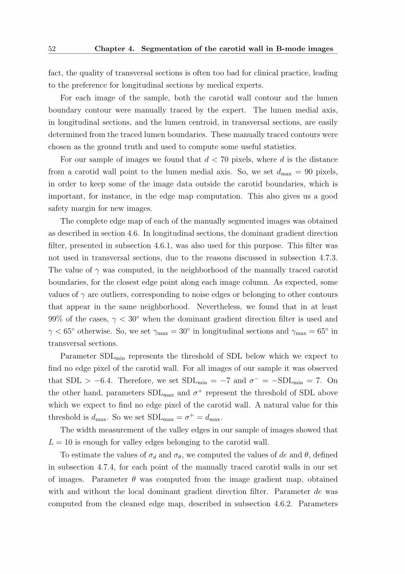
52 Chapter 4. Segmentation of the carotid wall in B-mode images
fact, the quality of transversal sections is often too bad for clinical practice, leading
to the preference for longitudinal sections by medical experts.
For each image of the sample, both the carotid wall contour and the lumen
boundary contour were manually traced by the expert. The lumen medial axis,
in longitudinal sections, and the lumen centroid, in transversal sections, are easily
determined from the traced lumen boundaries. These manually traced contours were
chosen as the ground truth and used to compute some useful statistics.
For our sample of images we found that d < 70 pixels, where d is the distance
from a carotid wall point to the lumen medial axis. So, we set dmax = 90 pixels,
in order to keep some of the image data outside the carotid boundaries, which is
important, for instance, in the edge map computation. This also gives us a good
safety margin for new images.
The complete edge map of each of the manually segmented images was obtained
as described in section 4.6. In longitudinal sections, the dominant gradient direction
filter, presented in subsection 4.6.1, was also used for this purpose. This filter was
not used in transversal sections, due to the reasons discussed in subsection 4.7.3.
The value of γ was computed, in the neighborhood of the manually traced carotid
boundaries, for the closest edge point along each image column. As expected, some
values of γ are outliers, corresponding to noise edges or belonging to other contours
that appear in the same neighborhood. Nevertheless, we found that in at least
99% of the cases, γ < 30 when the dominant gradient direction filter is used and
γ < 65 otherwise. So, we set γmax = 30 in longitudinal sections and γmax = 65 in
transversal sections.
Parameter SDLmin represents the threshold of SDL below which we expect to
find no edge pixel of the carotid wall. For all images of our sample it was observed
that SDL > −6.4. Therefore, we set SDLmin = −7 and σ− = −SDLmin = 7. On
the other hand, parameters SDLmax and σ+ represent the threshold of SDL above
which we expect to find no edge pixel of the carotid wall. A natural value for this
threshold is dmax. So we set SDLmax = σ+ = dmax.
The width measurement of the valley edges in our sample of images showed that
L = 10 is enough for valley edges belonging to the carotid wall.
To estimate the values of σd and σθ, we computed the values of de and θ, defined
in subsection 4.7.4, for each point of the manually traced carotid walls in our set
of images. Parameter θ was computed from the image gradient map, obtained
with and without the local dominant gradient direction filter. Parameter de was
computed from the cleaned edge map, described in subsection 4.6.2. Parameters

4.9. Results 53
σd and σθ are scales of Tukey’s functions. Therefore, they may be computed as
σd =√
5 [CMAD(de) + med(de)] and σθ =√
5 [CMAD(θ) + med(θ)], respectively.
We found the value σθ ≈ 11, when the dominant gradient filter is used, or σθ ≈ 36,
when this filter is not used. In both cases we found σd ≈ 4 since this parameter is
not significantly influenced by the gradient map.
Two parameters of the bail-out tests used in the RANSAC algorithm were also
determined from the image data base, in particular:
1. The limit for the angle, θ, between the intensity gradient and the normal to
the carotid wall model (spline or ellipse) at the sample points. Its value is
given by the threshold σθ, also used in the gain function and already discussed
above.
2. The maximum eccentricity, ε, allowed for an ellipse. We haven’t found any case
of a transversal section of the carotid with eccentricity above 0.7. So, an ellipse
is immediately rejected if ε ≥ 0.75, a threshold that includes a comfortable
safety margin. In other words, an ellipse is rejected if its minor axis is less
than approximately 66% of the major axis.
Some examples of the carotid walls segmented by our model are presented in
Fig. 4.14-4.16, including a case of successful segmentation in the presence of graph-
ical markings placed by the medical doctor during the image acquisition. In the
examples of Fig. 4.16, a comparison is made between the manual contours and the
ones obtained with our algorithm.
The value of the gain function (equation 4.16) obtained for the lower spline in
Fig. 4.14 (f) is an example of an underestimated probability of a good abscissa
due to the influence of a thick carotid plaque. In this case, the plaque region
pushes the lumen boundary away from the wall boundary, reducing the value of
the SDL factor (fourth fuzzy function) in the gain function. A consequence of this
underestimated probability is an increase in the number of samples analyzed by
the RANSAC algorithm, which means an increase in the confidence of the fitted
wall model, at the cost of some additional computational effort. The quality of the
segmentation is not affected. In fact, the segmentation result in this example is quite
good, illustrating the robustness of the algorithm to the presence of large plaques.
The gain function usually shows a weaker response in transversal sections be-
cause: a) in these sections the dominant gradient orientation filter is not used and,
therefore, the intensity gradient has a larger variability; b) the ellipse model is not

54 Chapter 4. Segmentation of the carotid wall in B-mode images
(a) (b)
(c) (d)
(e) (f)
(g) (h)
Fig. 4.14: Examples of segmented carotid walls in longitudinal B-scans of the CCA:a) Carotid with no plaque; b) Faded version of (a) and the best computed splines, inblack, above and below the lumen, with gain function Ga ≈ 71.3% and Gb ≈ 81.9%,respectively; c) Carotid with no plaque; d) Faded version of (c) and best splines, withGa ≈ 57.2% and Gb ≈ 68.9%; e) Carotid with extensive plaque; f) Faded version of(e) and best splines, with Ga ≈ 62.5% and Gb ≈ 54.0%; g) Carotid with plaque andgraphical markings placed during acquisition; h) Faded version of (g) and best splines,with Ga ≈ 45.7% and Gb ≈ 50.3%.
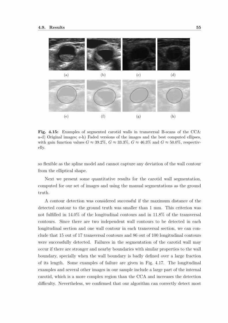
4.9. Results 55
(a) (b) (c) (d)
(e) (f) (g) (h)
Fig. 4.15: Examples of segmented carotid walls in transversal B-scans of the CCA:a-d) Original images; e-h) Faded versions of the images and the best computed ellipses,with gain function values G ≈ 39.2%, G ≈ 33.3%, G ≈ 46.3% and G ≈ 50.0%, respectiv-elly.
so flexible as the spline model and cannot capture any deviation of the wall contour
from the elliptical shape.
Next we present some quantitative results for the carotid wall segmentation,
computed for our set of images and using the manual segmentations as the ground
truth.
A contour detection was considered successful if the maximum distance of the
detected contour to the ground truth was smaller than 1 mm. This criterion was
not fulfilled in 14.0% of the longitudinal contours and in 11.8% of the transversal
contours. Since there are two independent wall contours to be detected in each
longitudinal section and one wall contour in each transversal section, we can con-
clude that 15 out of 17 transversal contours and 86 out of 100 longitudinal contours
were successfully detected. Failures in the segmentation of the carotid wall may
occur if there are stronger and nearby boundaries with similar properties to the wall
boundary, specially when the wall boundary is badly defined over a large fraction
of its length. Some examples of failure are given in Fig. 4.17. The longitudinal
examples and several other images in our sample include a large part of the internal
carotid, which is a more complex region than the CCA and increases the detection
difficulty. Nevertheless, we confirmed that our algorithm can correctly detect most

56 Chapter 4. Segmentation of the carotid wall in B-mode images
(a)
(b)
(c) (d)
Fig. 4.16: Example of manual (green) and automatic (red) contours of the CCA walls:a) Longitudinal section; b) Contours for the longitudinal section; c) Transversal section;d) Contour for the transversal section.

4.9. Results 57
of the wall boundaries. In appendices F and G, several other examples of successful
and unsucessful segmentations are presented.
The following statistics were computed for the successful segmentations. Fig-
ure 4.18 (a) gives the boxes and whiskers for the maximum distance error, Derr,
between the ground truth and the contour segmented automatically. This measure
shows the maximum deviation from the ground truth. It is reliable in the present
case, since the proposed segmentation model is robust to isolated outliers. In longi-
tudinal sections, Derr is computed twice, one measure for the upper boundary and
another for the lower one. In this case, the distance between the detected curve and
the ground truth curve is simply the vertical distance between these two curves at
each abscissa. In transversal sections, both the detected curve and the ground truth
are densely sampled. Then, for each point of the detected curve, the distance to the
ground truth is set as the smallest distance to the points of the ground truth.
Figure 4.18 (b) shows similar statistics for the relative area error, Aerr, defined
by the following expression
Aerr = 1 − A ∩ Aref
A ∪ Aref
(4.19)
where A is the area inside the automatically segmented contour and Aref is the area
of reference (the ground truth). This measure was used as a complement of Derr,
to evaluate the global quality of each segmentation. In longitudinal sections, Aerr
is computed only when both longitudinal contours were correctly detected, which
happened in 37 of the 50 longitudinal images in the sample. As expected, the error
is larger in transversal sections, where the wall boundaries are more likely to be
missing in the image. This increases the uncertainty in the location of the real
boundary, making it difficult to evaluate the real error. In general, a segmentation
of a transversal section can be considered acceptable if the ellipse fits the visible
contours reasonably well and gives an overall acceptable location of the boundary.
Although Matlab is not the best platform for efficiency, the CPU statistics pre-
sented in Fig. 4.19 give an idea of the relative computational weight of the main
tasks in the wall segmentation. The simulations were done with a PC equipped with
an Intel Core 2 Duo processor at 2.13 GHz and a 2GB RAM. The RANSAC algo-
rithm usually takes longer to segment transversal sections. This should not come
as a surprise, considering the lower quality of the wall boundaries and of the ellipse
fitting, when compared to the boundaries in longitudinal sections and the spline
fitting.

58 Chapter 4. Segmentation of the carotid wall in B-mode images
(a) (b)
(c) (d)
(e) (f)
Fig. 4.17: Examples of failure in the segmentation of the carotid wall: a) Longitudinalsection; b) Detected (red) and manually traced (green) wall contours for (a); c) Lon-gitudinal section; d) Detected (red) and manually traced (green) wall contours for (c)e) Transversal section; f) Detected (red) and manually traced (green) wall contour for (e).

4.9. Results 59
Transversal Longitudinal
0.2
0.4
0.6
0.8
Der
r (m
m)
(a)
Transversal Longitudinal
2
4
6
8
10
12
14
Aer
r (%
)
(b)
Fig. 4.18: Error statistics for the wall segmentation: a) Derr b) Aerr.
SF GDF RANSAC Total0
50
100
Tim
e (s
)
(a)
SF RANSAC Total0
50
100
Tim
e (s
)
(b)
Fig. 4.19: CPU statistics for the wall segmentation for the non-linear image smoothingfilter (SF), the dominant gradient direction filter (GDF), the RANSAC algorithm and thetotal time: a) Longitudinal sections; b) Transversal sections.

60 Chapter 4. Segmentation of the carotid wall in B-mode images
4.10 Concluding remarks
We have introduced a new algorithm for the segmentation of the carotid wall in both
longitudinal and transversal B-mode sections of the CCA. This algorithm looks for
the best smooth global path in the image, according to a newly proposed gain
function, which integrates the response to several discriminating characteristics of
the carotid wall in B-mode images. Our implementation of the RANSAC algorithm
makes the search of the best path more efficient.
The complete cubic spline and the ellipse proved to be good geometric model
priors for longitudinal and transversal sections, respectively. The 2D spline fitting
seems to be a better geometric model than the ellipse for the wall boundary in
transversal sections, but its computational complexity is too high.
Several presented examples and quantitative evaluations showed that our seg-
mentation algorithm is robust to the highly degrading factors typical of these images,
like the heavy noise, missing data and occlusions of the lumen region by plaque, pro-
ducing good estimates of the wall boundaries, comparable to the contours manually
traced by a specialist.
The results proved the high degree of discrimination of the selected characteris-
tics for the wall boundary. But some additional information is needed to improve
the robustness of the algorithm to other neighboring anatomical boundaries. This
missing information is probably of contextual or anatomical nature.

Chapter 5
SEGMENTATION OF THE CAROTID
LUMEN IN B-MODE IMAGES
5.1 Introduction
There are several properties of the B-mode images of the carotid that make the
automatic detection of the lumen very difficult, in particular: a) gaps in the carotid
boundaries due to echo dropouts are very common; b) there is usually a large echo
and contrast variability over the image domain; c) the noise inside the lumen may
be as strong as the echo produced by some parts of the tissues inside the carotid
wall; d) some plaques are hypoechogenic, appearing as very dark regions, making
its detection extremely difficult, even for a human observer.
Unfortunately, unlike the carotid wall, the lumen region cannot be represented by
a geometric prior due to the possible presence of plaque. Therefore, the shape-based
active contours are of no use here. We will keep to the simple active contour,
without any shape restriction, which is still very powerful and useful in the lumen
segmentation.
A new algorithm for an effective and automatic segmentation of the carotid lumen
in B-mode images is proposed. It combines the speed of thresholding algorithms
with the accuracy, flexibility and robustness of a successful geometric active contour
model.
The chapter begins with a small overview of the proposed algorithm. Several
thresholding algorithms are presented and tested in the segmentation of the lumen
in B-mode images. Then, the proposed algorithm is described in detail. The chapter
ends with a section of results, computed from an image data base, and a section of
concluding remarks.

62 Chapter 5. Segmentation of the carotid lumen in B-mode images
5.2 Overview of the approach
The proposed algorithm consists of three main steps. First, an estimate of the
lumen boundary contour is computed with a dynamic programming algorithm. This
estimated contour is usually a good approximation of the correct location of the
lumen boundary and is very fast to compute. Nevertheless, it is often rugged and
cannot capture all details of the lumen boundary when it has deep concavities or
sharp saliences. Therefore, an additional processing is needed to improve these
issues. This is done by a region-based geometric active contour.
The chosen active contour groups the image pixels according to their echo inten-
sity. Therefore, it requires the knowledge of an intensity threshold at each pixel of
the image. So, the estimation of this threshold is the second step of our algorithm.
A single intensity threshold usually produces poor results when the illumination of
an image is not constant. To cope with the intensity variability throughout the
image domain, a smooth thresholding surface is computed. It is derived from the
intensity values at the edge pixels that belong to the contour obtained with the
dynamic programing algorithm.
Finally, a two-phase piecewise constant geometric active contour [97, 98] is ini-
tialized at the location estimated by the dynamic programming algorithm. Then, it
evolves in the image plane according to the intensity topology and the thresholding
surface. The active contour reduces the noise, produces smoother estimates of the
lumen boundary and improves its position accuracy.
To avoid leakage through large gaps in the carotid boundary, the evolution of
the active contour is restrained to the region inside the previously segmented wall
contour.
5.3 Thresholding
Thresholding is one of the most popular segmentation approaches for images in
which the objects of interest have different intensity from the background. It has
the advantages of being very fast and frequently producing quite good segmentation
results. Therefore, we thought it would be interesting to evaluate its performance
in the segmentation of the carotid lumen in B-mode images.
The number of published thresholding algorithms is so large that it would be an
enormous effort to evaluate them all. A very comprehensive and recent survey can
be found in [99]. In this work, the authors used several figures of merit to evaluate

5.3. Thresholding 63
the performance of each thresholding algorithm and ranked them according to their
overall average quality score. Two ranking tables were presented, one for document
images and another for non-document images. We selected several algorithms be-
tween the best 10 in the rank presented for non-document images, in particular:
Kittler’s algorithm [100] (1st in the rank); Kapur’s algorithm [101] (2nd in the rank);
Sahoo’s algorithm [102] (3rd in the rank); Yen’s algorithm [103] (4th in the rank);
Otsu’s algorithm [104] (6th in the rank); Yanowitz’s algorithm [105] (8th in the rank);
Li’s algorithm [106] (10th in the rank).
Some of the listed algorithms were chosen not only for their good ranking posi-
tion but also due to some particular properties that make them attractive for our
application. The Otsu’s algorithm was included for being a very popular model,
usually used as a reference to compare other algorithms. Yanowitz’s algorithm was
the local thresholding algorithm with the highest score. In fact, it was the only one
of its group to appear in the first 20 places. It was chosen because its local approach
makes it more effective for images with poor and nonuniform illumination. Finally,
Li’s algorithm is known to produce better segmentations than most other single
global thresholding algorithms, when some assumptions about the populations’ dis-
tributions, size and variance are not valid [106].
To this list of selected thresholding algorithms, we added the triangle algorithm
[86, 107], which is known to work well when the image histogram has a single large
peak and a long tail, as is typical of B-mode images of the carotid. Two new
algorithms were conceived and tested, in particular, the sequential and the local
minimum cross entropy algorithms.
With the exception of the Otsu’s algorithm, which is available in Matlab’s image
processing toolbox, all these thresholding algorithms were implemented in Matlab.
The rest of this section gives a brief description of each of the selected algorithms,
as well as examples of their application to B-mode images of the carotid. At the
end of the chapter, some statistics will be presented for their performance in these
images.
Now we introduce some notation and important definitions. LetN be the number
of image pixels, G = 0, 1, 2, . . . , L − 1 the set of intensity levels in the gray scale
image, k ∈ G an intensity level, and h(k) the image histogram. The probability,
p(k), of intensity k in the image, the total intensity mean, µ, and the total intensity
variance, σ2, are given by:
p(k) =h(k)
N(5.1)

64 Chapter 5. Segmentation of the carotid lumen in B-mode images
µ =L−1∑
k=0
kp(k) (5.2)
σ2 =L−1∑
k=0
(k − µ)2p(k) (5.3)
Let T be the intensity threshold that segments the image into two classes, C1 =
(x, y) : 0 ≤ k ≤ T and C2 = (x, y) : T < k < L. A useful quantity is
µ(T ) =T
∑
k=0
kp(k) (5.4)
Finally, the probability of class one, P1(T ), the probability of class two, P2(T ), the
intensity mean of each class, µ1(T ) and µ2(T ), and their intensity variances, σ21(T )
and σ22(T ), are given by
P1(T ) =T
∑
k=0
p(k), P2(T ) =L−1∑
k=T+1
p(k) = 1 − P1(T ) (5.5)
µ1(T ) =
∑T
k=0 kp(k)
P1(T ), µ2(T ) =
∑L−1k=T+1 kp(k)
P2(T )=
µ− µ(T )
1 − P1(T )(5.6)
σ21(T ) =
∑T
k=0 [k − µ1(T )]2 p(k)
P1(T ), σ2
2(T ) =
∑L−1k=T+1 [k − µ2(T )]2 p(k)
P2(T )(5.7)
5.3.1 Otsu’s method
Otsu’s algorithm [104] assumes a bimodal histogram and similar populations and
variances for both classes. It looks for the intensity threshold, T , that maximizes
the separability of the two classes, measured by one of the following equivalent
criteria: λ = σ2B/σ
2W or η = σ2
B/σ2 or κ = σ2/σ2
W, where σ2 is the total variance
of the image, σ2B = P1(T )P2(T ) [µ1(T ) − µ2(T )]2 is the variance between classes
and σ2W = P1(T )σ2
1(T ) + P2(T )σ22(T ) is the variance within classes. The optimum
threshold, Topt, can be computed in a very efficient way as
Topt = arg maxT∈G
η(T )
= arg maxT∈G
[µP1(T ) − µ(T )]2
σ2P1(T )[1 − P1(T )]
(5.8)

5.3. Thresholding 65
(a) (b)
(c) (d)
Fig. 5.1: Examples of Otsu’s thresholding: a) B-mode image of the carotid with insignif-icant speckle noise in the lumen; b) Binary image produced by the Otsu’s threshold forimage (a); c) B-mode image of the carotid with some speckle noise in the lumen; b) Binaryimage produced by the Otsu’s threshold for image (c)
Two segmentation examples are presented in Fig. 5.1, one for an image with
some speckle noise inside the lumen and another for an image with insignificant
speckle noise in the lumen.
5.3.2 Kittler’s method
Kittler’s algorithm [100] assumes the image histogram is a mixture of two Gaussian
distributions, one for foreground pixels and the other for background pixels. It also
assumes that the overlap between the two underlying distributions is small. This
overlap tends to introduce a bias in the estimated threshold and, if it is too large, it
may lead to a complete failure of the algorithm. The optimum threshold is the one
that minimizes the total misclassification error and can be obtained as
Topt = arg minT∈G
1 + 2 [P1(T )ln σ1(T ) + P2(T )ln σ2(T )]
− 2 [P1(T )ln P1(T ) + P2(T )ln P2(T )]
(5.9)

66 Chapter 5. Segmentation of the carotid lumen in B-mode images
(a) (b)
Fig. 5.2: Binary images produced by the Kittler’s algorithm: a) For the image inFig. 5.1 (a); b) For the image in Fig. 5.1 (c).
or, in a simpler and equivalent way, as
Topt = arg minT∈G
P1(T )ln σ1(T ) + P2(T )ln σ2(T )
− P1(T )ln P1(T ) − P2(T )ln P2(T )
(5.10)
Two segmentation examples are presented in Fig. 5.2.
5.3.3 Kapur’s method
Kapur’s algorithm [101] maximizes the information measure between classes C1 and
C2, viewed as two different signal sources. It is also known as the maximum entropy
sum method because the optimum threshold is the one that maximizes the sum of
the Shanon entropies for the two classes. These class entropies are defined as
H1(T ) = −T
∑
k=0
p(k)
P1(T )ln
p(k)
P1(T )
H2(T ) = −L−1∑
k=T+1
p(k)
P2(T )ln
p(k)
P2(T )
(5.11)
and the optimum threshold is given by
Topt = arg maxT∈G
H1(T ) +H2(T )
= arg maxT∈G
ln [P1(T )P2(T )] +H(T )
P1(T )+HT −H(T )
P2(T )
(5.12)

5.3. Thresholding 67
(a) (b)
Fig. 5.3: Binary images produced by the Kapur’s algorithm: a) For the image inFig. 5.1 (a); b) For the image in Fig. 5.1 (c).
where
H(T ) = −T
∑
k=0
p(k)ln p(k) (5.13)
and HT is the entropy for the entire image, given by
HT = −L−1∑
k=0
p(k)ln p(k) (5.14)
Two segmentation examples are presented in Fig. 5.3.
5.3.4 Sahoo’s method
This method, introduced in [102], uses the Renyi’s entropy, defined as
HαR =
1
1 − αln
M∑
i=1
pαi (5.15)
where α (6= 1) is a positive real number. This entropy is a one parameter general-
ization of the Shannon entropy, HS = −∑M
i=1 piln pi, since limα→1HαR = HS [102].
The particular case of α = 1 corresponds to the Kapur’s algorithm. The optimum
threshold is a weighted average of three different thresholds, each of which maxi-
mizes the sum of the Renyi’s entropy of the two classes for a particular value of α.
The first value of α is in 0 < α < 1, the second is α = 1 and the third comes from

68 Chapter 5. Segmentation of the carotid lumen in B-mode images
(a) (b)
Fig. 5.4: Binary images produced by the Sahoo’s algorithm: a) For the image inFig. 5.1 (a); b) For the image in Fig. 5.1 (c).
range α > 1. The Renyi’s entropies for classes C1 and C2 are defined as
Hα1 (T ) =
1
1 − αln
T∑
k=0
(
p(k)
P1(T )
)α
Hα2 (T ) =
1
1 − αln
L−1∑
k=T+1
(
p(k)
P2(T )
)α(5.16)
and the optimum threshold for a given value of parameter α is given by
Topt(α) = arg maxT∈G
Hα1 (T ) +Hα
2 (T ) (5.17)
Two segmentation examples are presented in Fig. 5.4, where the three thresholds
used in the final average (with the weights proposed in [102]) were computed for
α = 0.5, α = 1 and α = 2.
5.3.5 Yen’s method
Yen’s method [103] maximizes the sum of the Renyi’s entropies of the two classes,
using equation 5.17 with α = 2. Two segmentation examples are presented in
Fig. 5.5.
5.3.6 Triangle method
As illustrated in Fig. 5.6, the triangle algorithm [86] starts by determining the line
passing through points (ka, h(ka)) and (kb, h(kb)), the peak of the histogram and
the end of the histogram tail, respectively. The distance, d, from this line to the

5.3. Thresholding 69
(a) (b)
Fig. 5.5: Binary images produced by the Yen’s algorithm: a) For the image in Fig. 5.1 (a);b) For the image in Fig. 5.1 (c).
k
h(k) d
dmax
kopt
(ka, h(ka))
(kb, h(kb))
Fig. 5.6: The triangle algorithm selects the intensity threshold (kopt) that maximizes thedistance d.
histogram is computed for each intensity, between ka and kb. The optimum thresh-
old is selected as the intensity that maximizes the value of d. Two segmentation
examples are presented in Fig. 5.7.
5.3.7 Minimum cross entropy method
The minimum cross entropy (MCE) algorithm [106] minimizes the cross entropy
between the gray scale image and its binary version obtained with a threshold, T .
The cross entropy, also known as Kullback’s distance, measures the information
theoretic distance between two given distributions, P = p1, p2, . . . , pM and Q =
q1, q2, . . . , qM, and is expressed as
D(Q,P ) =M
∑
i=1
qiln(qipi
) (5.18)

70 Chapter 5. Segmentation of the carotid lumen in B-mode images
(a) (b)
Fig. 5.7: Binary images produced by the triangle algorithm: a) For the image inFig. 5.1 (a); b) For the image in Fig. 5.1 (c).
(a) (b)
Fig. 5.8: Binary images produced by the MCE algorithm: a) For the image in Fig. 5.1 (a);b) For the image in Fig. 5.1 (c).
This distance is minimized under the constraint that both the segmented and
the binary image have identical intensity means in their foreground and background,
which leads to the following equation
Topt = arg minT∈G
T∑
k=0
kh(k)ln
(
k
µ1(T )
)
+L−1∑
k=T+1
kh(k)ln
(
k
µ2(T )
)
(5.19)
where we assume that 0 ln(0) = 0.
Two segmentation examples are presented in Fig. 5.8.
Unlike other algorithms that make assumptions about the distribution and vari-
ances of the two classes present in the image, the MCE criterion gives threshold
estimates without the tendency of biasing when these assumptions are not true.
This is probably the reason why it performs better, in our images, than most of the
other tested thresholding algorithms (see the statistics in section 5.6). In the group
of single global thresholding, the MCE algorithm was only surpassed by the triangle
5.3. Thresholding 71
algorithm. This is the reason behind its choice in two other thresholding algorithms
proposed next, in particular, the sequential minimum cross entropy algorithm and
the local minimum cross entropy algorithm.
5.3.8 Sequential minimum cross entropy method
Due to the echo variability in B-mode images, their segmentation may be viewed
as a multiphase problem in which the lumen is a part of the darkest phase in the
image. This assumption is made in [13] to present a new thresholding algorithm,
called sequential minimum cross entropy (SMCE).
The idea behind the SMCE thresholding is to use the MCE algorithm iteratively.
In the first iteration, the MCE algorithm is used to divide the original image into two
regions. In the second iteration, the darkest region produced by the first iteration is
further subdivided into another pair of regions, and so on, until a certain stopping
criterion is satisfied. At the end of each iteration, only two regions of interest
remain: the region with intensities below the last threshold and the region with all
other intensities.
If the lumen has low noise, it appear as a very dark and homogeneous region, for
which the intensity standard-deviation, σ, is quite small. This information can be
used in a stopping criterion. Iterations come to an end when the value of σ, for the
darkest region in the last iteration, drops bellow a certain threshold. Segmentation
examples with this iterative algorithm, using σ < 0.01 as stopping criterion, are
presented in Fig. 5.9. This works well if there is no significant noise inside the
lumen. Otherwise, it will usually stop too late, as in the example presented in
Fig. 5.9 (b), where some of the lumen noise is classified as other tissue. A possible
solution would be to automatically adapt the σ threshold to each image, according
to the level of noise expected in the lumen region. But no reliable criterion was
found to do this.
5.3.9 Local minimum cross entropy method
An alternative to the SMCE algorithm is a local MCE (LMCE), which uses a single
MCE threshold computed only for the region inside the carotid. The carotid bound-
ary is included in the support region to make sure we always keep some other tissue
besides the blood in the lumen. The local support of the thresholding gives a better
estimate of the lumen region than most of the other tested thresholding algorithms.
Figure 5.10 shows the binary images obtained with the LMCE algorithm for the gray

72 Chapter 5. Segmentation of the carotid lumen in B-mode images
(a) (b)
Fig. 5.9: Binary images produced by the SMCE algorithm: a) For the image inFig. 5.1 (a); b) For the image in Fig. 5.1 (c).
(a) (b)
Fig. 5.10: Binary images produced by the LMCE algorithm: a) For the image inFig. 5.1 (a); b) For the image in Fig. 5.1 (c).
scale images presented in Fig. 5.1. One limitation of this approach is that it can
only be applied after the segmentation of the carotid wall contours, since it needs
this information to compute the boundaries of the support region.
5.3.10 Yanowitz’s method
In spite of the apparent acceptable performance of some of the above methods (in
particular, the triangle and the LMCE algorithm), all the considered single threshold
methods give very poor results when the intensity variability becomes large. As
can be seen in the example of Fig. 5.11, large extensions of the plaque region are
misclassified as a part of the lumen, by both the triangle and the LMCE algorithms,
due to the nonuniform and very weak echo produced by the plaque. On the other
hand, some noise inside the lumen appears as white regions in the binary image.
Obviously, this problem requires local thresholding.
The approach followed by Yanowitz and Bruckstein [105] is quite different from

5.3. Thresholding 73
(a) (b) (c)
Fig. 5.11: Thresholding an image with a dark plaque and nonuniform illumination:a) Ultrasound image with nonuniform illumination and a dark plaque; b) Segmentationobtained with the triangle thresholding algorithm; c) Segmentation obtained with theLMCE thresholding algorithm.
(a) (b) (c)
Fig. 5.12: Thresholding with nonuniform illumination: a) Image with nonuniform illumi-nation; b) Segmentation obtained with the Otsu’s thresholding algorithm; c) Segmentationobtained with the Yanowitz’ thresholding algorithm.
the methods described so far. Instead of a single intensity threshold for the en-
tire image, a local threshold is computed for each image pixel, in the form of a
smooth thresholding surface. This is a generalization of the single global threshold-
ing approach, which is equivalent to using a thresholding surface with a constant
height. Local thresholding methods may produce better segmentations when the
image presents nonuniform illumination. As an example, Fig. 5.12 shows an image
with nonuniform illumination, as well as the binary image produced by the Otsu’s
algorithm, where we can see that the objects at the darker part of the image are
not well detected. Figure 5.12 (c) shows the segmentation improvement introduced
by Yanowitz’ algorithm.
In [105], the thresholding surface is determined by interpolating the image in-
tensities at edge pixels, where we expect to find intensity values that are good local

74 Chapter 5. Segmentation of the carotid lumen in B-mode images
thresholds. The algorithm may be summarized in the following steps:
1. A low-pass filter is applied to the image to obtain a smoothed version, with
reduced noise and moderate slopes at edges. This improves the estimates of
the local thresholds.
2. An edge map is computed from the smoothed image as the local maxima of
the gradient magnitude in the gradient direction, above a certain threshold.
3. The edge pixels found at the image boundaries are used to estimate, by linear
interpolation, the intensity thresholds along the whole image border. This
step is required for a good segmentation of objects that are cut by the image
frame.
4. The intensities at the edge pixels and the intensity thresholds estimated at the
image boundaries are interpolated over the rest of the image, by solving the
Laplace’s equation∂2u
∂x2+∂2u
∂y2= 0 (5.20)
for the thresholding surface, u.
5. The solution of this equation will be our smooth thresholding surface, which
can then be used to segment the image.
6. If the thresholding surface intersects the image intensity surface inside the
objects or the background, ’ghost’ objects will appear in the binary image.
These stains may be removed by a validation process, where white or black
regions are eliminated if they have a weak edge support along their boundary.
The surfaces that satisfy equation 5.20 are known as potential surfaces and their
smoothness comes from the fact that the divergence of their gradient vanishes ev-
erywhere [105].
Our implementation of this algorithm has some differences relative to the one
proposed in [105], as discussed next.
We implemented two versions of the algorithm. The first one uses the Canny’s
edge detector [67], where a Gaussian filter is used to smooth the image and the
gradient magnitude is used to measure the edge strength. This should be more
appropriate for images with additive noise. The second version uses the non-linear
smoothing filter proposed in section 4.5 and the ICOV-based edge detector described
in section 4.6. This version is better suited for ultrasound images, where the noise

5.3. Thresholding 75
(a) (b)
Fig. 5.13: Interpolating data in Yanowitz’ algorithm: a) Edge map for the image inFig. 5.12 (a); b) Intensities at the interpolating pixels for the same image, where a higherimage intensity is represented by a darker pixel.
has a multiplicative nature. Non-maxima suppression and hysteresis are used in
both versions. In practice, the smoothed image (step 1) and the corresponding edge
map (step 2) are previously computed, using independent functions that are also
useful to other applications, and then passed to the next steps of the Yanowitz’
algorithm.
The second difference is in the intensity (linear) interpolation along the image
border. In [105], only the edge points detected at the image boundaries are used in
this interpolation. To improve its reliability, we extended the search for edge points
to the 8-neighborhood of image boundary pixels. In Fig. 5.13 we can see the edge
map of the image in Fig. 5.12 and the intensities at all interpolating pixels, that is,
the pixels at the detected edges and the images borders.
Another important difference is the resolution of the Laplace’s equation. Its
solution is computed in two steps. First, an approximate solution is obtained with a
very fast algorithm that propagates the intensity values at the interpolating pixels
to the rest of the image pixels. Second, the Laplace’s equation is solved with the
following numerical scheme
un+1i,j = 0.25
(
uni+1,j + un
i−1,j + uni,j+1 + un
i,j−1
)
un+1i,j = λun+1
i,j + (1 − λ)uni,j, n = 0, 1, 2, . . .
(5.21)
where uni,j is the value of the thresholding surface at pixel (i, j) and iteration n,
λ = 1.5 and the initial solution, u0, is the surface obtained in the first step.
The second equality of equation 5.21 introduces over-relaxation [94] to speed up

76 Chapter 5. Segmentation of the carotid lumen in B-mode images
(a) (b) (c)
Fig. 5.14: Thresholding surfaces for the interpolating data in Fig. 5.13 (b), where thesurface value at each pixel is represented by a gray scale level: a) Solution of the Laplace’sequation if the initial values of the interpolated pixels are set to zero; b) Surface obtained bypropagating the intensities at the interpolating pixels to the rest of the image; c) Solutionof the Laplace’s equation if the initial solution is the surface presented in (b).
the convergence. The iterations stop when the relative intensity difference between
two consecutive iterations is less than 1% for all image pixels.
The intensity propagation step was implemented as described next. The Eu-
clidean distance map to the interpolating pixels is computed with a very fast al-
gorithm [88]. Then, the other pixels are ordered in a list by ascending value of
the computed distance and processed in that order. At each pixel in the list, the
intensity threshold is computed as a weighted average of the thresholds found for its
8-neighbors with smaller distance to the data points. The weights used in the aver-
age are inversely proportional to the distances of the central pixel to its 8-neighbors.
As can be seen in Fig. 5.14 (b), this solution is not as smooth as desired, but
its computation is extremely fast and will significantly reduce the total computa-
tional effort, when used to initialize the numerical scheme for the Laplace’s equation.
Moreover, initializing the interpolated pixels with zero will usually lead to solutions
with deeper concavities, which are more likely to produce ’ghost’ objects in the bi-
nary image obtained through thresholding. Figure 5.14 (a) and Fig. 5.14 (c) show
the solutions obtained for the Laplace’s equation when initializing the interpolated
pixels with zeros and with the propagated intensities, respectively. The solution of
Fig. 5.14 (a) has darker regions between the interpolating pixels, evidencing deeper
concavities of the thresholding surface in those areas.
Finally, Fig. 5.15 presents two examples of the segmentation produced by this al-
gorithm in B-mode images, without the validation step used to remove false objects.
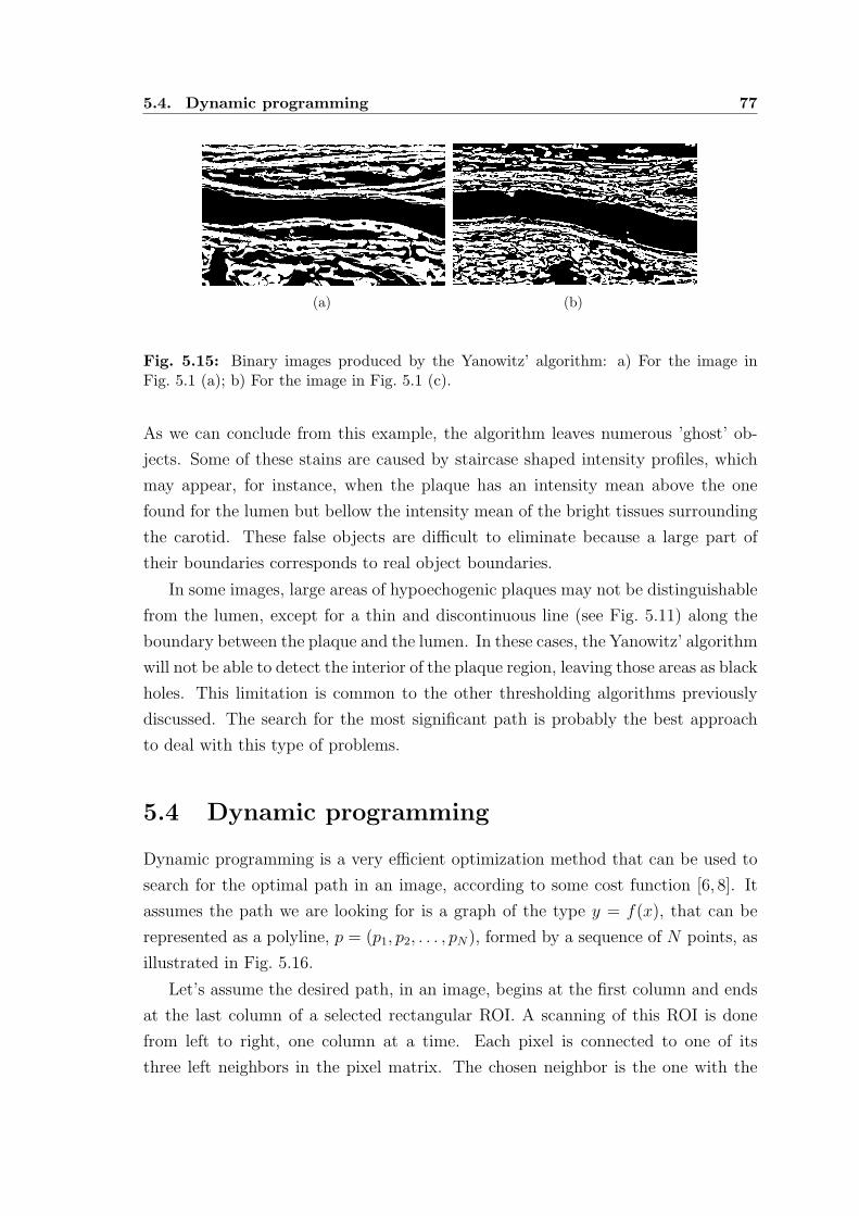
5.4. Dynamic programming 77
(a) (b)
Fig. 5.15: Binary images produced by the Yanowitz’ algorithm: a) For the image inFig. 5.1 (a); b) For the image in Fig. 5.1 (c).
As we can conclude from this example, the algorithm leaves numerous ’ghost’ ob-
jects. Some of these stains are caused by staircase shaped intensity profiles, which
may appear, for instance, when the plaque has an intensity mean above the one
found for the lumen but bellow the intensity mean of the bright tissues surrounding
the carotid. These false objects are difficult to eliminate because a large part of
their boundaries corresponds to real object boundaries.
In some images, large areas of hypoechogenic plaques may not be distinguishable
from the lumen, except for a thin and discontinuous line (see Fig. 5.11) along the
boundary between the plaque and the lumen. In these cases, the Yanowitz’ algorithm
will not be able to detect the interior of the plaque region, leaving those areas as black
holes. This limitation is common to the other thresholding algorithms previously
discussed. The search for the most significant path is probably the best approach
to deal with this type of problems.
5.4 Dynamic programming
Dynamic programming is a very efficient optimization method that can be used to
search for the optimal path in an image, according to some cost function [6, 8]. It
assumes the path we are looking for is a graph of the type y = f(x), that can be
represented as a polyline, p = (p1, p2, . . . , pN), formed by a sequence of N points, as
illustrated in Fig. 5.16.
Let’s assume the desired path, in an image, begins at the first column and ends
at the last column of a selected rectangular ROI. A scanning of this ROI is done
from left to right, one column at a time. Each pixel is connected to one of its
three left neighbors in the pixel matrix. The chosen neighbor is the one with the

78 Chapter 5. Segmentation of the carotid lumen in B-mode images
Fig. 5.16: A polyline, represented by the curve connecting the red points.
lowest accumulated value of the cost function, up to the previous column. After
the connection is made, the accumulated value of the cost function at the current
pixel is computed and stored. At the last column of the ROI, each pixel is the end
point of a polyline. The other points of each polyline can be found by backtracking
through the pointers to the best left neighbors, up to the first column of the matrix.
The optimal path is the one that minimizes the total cost function
Ct =N
∑
j=1
c(pj) (5.22)
where
c(pj) =m
∑
k=1
wkψk(pj) (5.23)
is the local cost of the path at its point pj, defined as a weighted sum of m local cost
terms, ψk(pj), reflecting the influence of different image local features or geometrical
properties. The weight factors, represented by wk, determine the relative importance
of each local cost term.
Representing by C(pn) =∑n
j=1 c(pj) the accumulated cost at point pn, we can
rewrite equation 5.22 in the following recursive form
C(p1) = c(p1)
C(pj) = C(pj−1) + c(pj), j = 2, 3, . . . , N(5.24)
Therefore, at each pixel, pi,j, the accumulated cost, C(pi,j), and the pointer to the
best left pixel can be stored in position (i, j) of two arrays with the same size of the
ROI.
There are several image features that can be integrated into the cost function,
depending on the application. In [6], a cost function was proposed to detect the

5.4. Dynamic programming 79
boundaries of the carotid in B-mode images. It consists of three terms, one related
to an echo intensity feature, another related to an intensity gradient feature and,
finally, a geometric constraint term. This model and its disadvantages were already
discussed in section 3.1.
We introduce a new approach that gives satisfactory results and has the advan-
tage of using the ICOV strength instead of the gradient magnitude.
The geometric term was implemented as a function of the length of the path,
since this constraint is the most frequent in some very successful models for active
contours [97,98].
Although we could easily include, as well, an echo intensity term, we tried to
avoid it to keep the model as simple as possible, with the advantage of requiring the
estimation of less weights.
Our algorithm can be summarized in the following steps:
1. Compute the strong edge map, Estrong, as described in section 4.6, for the
ROI selected during the segmentation of the carotid wall. Figure 5.17 shows
an example of an image ROI for a longitudinal section and the corresponding
strong edge map, where we can see that significant parts of the lumen boundary
were not detected.
2. Using a similar procedure, compute the edge map with all edges, Eall, including
the weak ones. An example is presented in Fig. 5.18 (a). This edge map is
important because we have noticed that large parts of the lumen boundary
may be far too weak to be captured in the strong edge map. In fact, some of
the recovered lumen boundary edges are virtually imperceptible to a human
observer.
3. Create a new edge map, E, containing only the edges of Eall that fall strictly
inside the carotid wall. See Fig. 5.18 (b).
4. Clean all edges with incompatible gradient direction (Fig. 5.19). The lumen
region is darker than the surrounding tissues. So, as in subsection 4.6.2, we
should clean the edge maps from all edges with gradient pointing to the interior
of the artery, i.e., with a large value of the angle γ. Since the lumen boundary
can be much more irregular than the carotid wall, we are less demanding here,
removing only the edges with γ ≥ 90.
5. Normalize, over each vertical or radial line segment, the ICOV of the edges in
E. Starting from the lumen axis, we walk along the line segment, searching

80 Chapter 5. Segmentation of the carotid lumen in B-mode images
(a) (b)
Fig. 5.17: a) ROI from a B-mode image of a longitudinal section; b) Edge map, Estrong,containing only strong edges.
for edges in E. For each of the line segments, the ICOV of each edge is divided
by the maximum value found for the edges in that segment. This procedure
gives a chance to the usually weaker lumen boundary edges to compete with
the wall edges. Otherwise, the polyline will usually be attracted toward the
wall, where the ICOV is much stronger.
6. Add to edge map E the strong edges that are visible from the lumen axis
(Fig. 5.20), normalizing their ICOV to one. These edges are the first ones
found in the cleaned strong edge map, starting at the lumen axis and walking
in the radial direction. This step is required because, when the intima-media
region (the one that separates the lumen from the carotid wall) is not visible,
the carotid wall is the best estimate of the lumen boundary.
7. Using dynamic programming, look for the path in E that minimizes the fol-
lowing cost function
Ct = ψ1(p1) +N
∑
j=2
[ψ1(pj) + λψ2(pj−1, pj)] (5.25)
where: ψ1(pj) = 1 − ICOV∗, if pj is an edge pixel of E, and ψ1(pj) = 1,
otherwise, where ICOV∗ represents the normalized ICOV as described in the
previous steps; ψ2(pj−1, pj) = 1/√
2, if pj−1 and pj belong to the same line in
matrix E, and ψ2(pj−1, pj) = 1, otherwise; λ is the weight of the geometric
term.

5.4. Dynamic programming 81
(a) (b)
Fig. 5.18: a) Complete edge map, Eall, containing all edges (strong and weak) found inthe image presented in Fig. 5.17; b) Edge map, E, with the edges in Eall that fall strictlyinside the carotid wall.
(a) (b)
Fig. 5.19: Edge maps after cleaning the edges with incompatible gradient direction:a) Cleaned version of the strong edge map, Estrong, presented in Fig. 5.17; b) Cleanedversion of the edge map, E, presented in Fig. 5.18.
(a) (b)
Fig. 5.20: a) Edges of Estrong that are visible from the lumen axis (curve in red) specifiedby the user; b) Final version of edge map, E, after adding to it the edges presented in (a).

82 Chapter 5. Segmentation of the carotid lumen in B-mode images
(a) (b)
Fig. 5.21: Lumen boundaries for the image in Fig. 5.17, segmented with dynamic pro-gramming: a) Without any geometric constraint (λ = 0); b) With a geometric constraint(λ = 5).
5.4.1 Dynamic programming for longitudinal sections
If the image corresponds to a longitudinal section of the carotid, we expect to find
two contours, one above and the other below the lumen medial axis. Both contours
start at the first column and finish at the last column of the edge map E. Therefore,
the dynamic programming algorithm can be applied directly to E. However, the
search must be done separately above and bellow the lumen medial axis. Figure 5.21
shows the lumen boundaries detected by our dynamic programming algorithm for
the image presented in Fig. 5.17. The example shows the results obtained with
(λ = 5) and without (λ = 0) a geometric constraint, to illustrate the smoothing
introduced by the geometric term. Similar results for the image of Fig. 5.11 are
presented in Fig. 5.22, to demonstrate the significant improvement relative to the
segmentation with thresholding algorithms, for hypoechogenic plaques.
5.4.2 Dynamic programming for transversal sections
In a transversal section, we have a single closed contour. To be able to apply the de-
scribed dynamic programming algorithm to this case, we select the smallest circular
region, centered at the lumen centroid specified by the user (see section 4.3), that
contains all the edges found in E. Then, we convert this ROI to polar coordinates,
(r, θ), to obtain a rectangular grid with size M × N . We set M = ceil(R) and
N = ceil(2πR), where R is the largest distance from an edge to the centroid and
ceil(z) is the smallest integer above a real value z. The angle θ ∈ [0, 2π] is divided
into N − 1 intervals of equal amplitude, such that the first and last columns of this
polar matrix correspond to θ = 0 and θ = 2π, respectively. The lines of this matrix
correspond to consecutive integer values of the radius, r, between 1 and M .

5.4. Dynamic programming 83
(a) (b)
Fig. 5.22: Lumen boundaries for the image in Fig. 5.11, segmented with dynamic pro-gramming: a) Without any geometric constraint (λ = 0); b) With a geometric constraint(λ = 5).
The polar version of E and of the ICOV map are computed using inverse map-
ping, from the polar system, (r, θ), to the cartesian system, (x, y), and selecting the
highest value of the pixels surrounding the point (x, y).
When the best path is determined in the polar system, it is converted to the
cartesian system through direct mapping. Each polar pixel is mapped to a single
cartesian point, (x, y). Then, we choose the neighboring cartesian pixel with the
highest ICOV. An alternative would be to round the coordinates of the cartesian
points, but the final curve would not be so smooth and its location would be less
accurate. Unlike inverse mapping, direct mapping may leave out some pixels of the
cartesian curve. However, inverse mapping would produce thicker lines, reducing
the accuracy of the boundary location. Besides, the gaps left by the direct mapping
are quite small and do not hinder the determination of the cartesian curve.
The dynamic programming algorithm frequently produces open contours, when-
ever the end points of the best polyline are located at different lines (radius) of
the polar matrix. To make sure the path is closed, we introduced the following
additional processing. Let iopt1 and iopt
N be the lines of the first and last polar pixels
of the optimum polyline, computed with the dynamic programming algorithm. We
repeat the backtracking of the best path, but this time starting at line iopt1 of the last
column. The new path will quickly converge to the initial best path, resulting in a
closed curve that contains most of the points of the initial polyline. Figure 5.23 gives
an example of the computed best path for a transversal section, with and without
the extra processing used to close the curve.

84 Chapter 5. Segmentation of the carotid lumen in B-mode images
(a) (b) (c)
Fig. 5.23: Detection of the lumen boundary in a transversal section, with dynamicprogramming and λ = 0: a) B-mode image of a transversal section; b) Contour obtainedby applying the dynamic programming algorithm to the polar grid; c) Contour given bythe proposed additional processing, to close the curve.
5.4.3 Weight of the geometric term in the cost function
The geometric constraint may help to avoid deviations from the lumen contour when
it is too weak and degraded, as in the example of Fig. 5.24. But this improvement
usually requires a very large weight of the geometric term, to overcome the stronger
ICOV of the alternative path. The lumen contour must have low curvature at those
degraded sections, otherwise, using a strong geometric constraint will introduce
more damage than improvement. A strong geometric weight and a lumen boundary
with high curvature do not mix well, often resulting in some undesired bypasses
through tissue or lumen regions, even when the edge strength is high at the bypassed
sections of the boundary. Two examples of this problem are presented in Fig. 5.25.
Unfortunately, lumen boundaries frequently contain segments with large curvature,
due to plaque formation. In face of this dilemma, we thought it would be more
acceptable not to detect some very degraded lumen boundary edges than to sacrifice
well defined parts of the boundary that have large curvature. Therefore, we chose to
drop the geometric constraint, by setting λ = 0 in the cost function. The roughness
of the detected contour can easily be eliminated though a posterior smoothing, with
an algorithm better suited for this purpose.
The segmentations produced for the image in Fig. 5.25 (d) illustrate quite well
another limitation of the algorithm. It cannot correctly detect deep concavities nor
sharp saliences, specially when they are oriented to the left or to the right, as in the
left part of the upper boundary. This limitation is intrinsic to the dynamic program-
ming approach, where the path does not invert the direction of its course during its

5.5. Smoothing the detected lumen boundaries 85
(a) (b)
(c) (d)
Fig. 5.24: Improved detection due to the geometric term: a) B-mode image of a lon-gitudinal section; b) Detected lumen boundaries (red) with λ = 0 and the ground truth(green); c) Detected lumen boundaries (red) with λ = 4 and the ground truth (green);d) Detected lumen boundaries (red) with λ = 5 and the ground truth (green).
construction. Nevertheless, it is possible to significantly reduce this error through
a region-based active contour, which is also used to produce smoother curves. The
proposed solution is discussed next.
5.5 Smoothing the detected lumen boundaries
The output of the dynamic programming algorithm presented above is frequently
not smooth enough. One simple and very fast solution to this problem is to fit,
to the pixels of each computed polyline, a weighted cubic smoothing spline [108],
with weights proportional to the value of the ICOV at each pixel. This should be
enough if the polyline, produced by the dynamic programming algorithm, closely
approximates the lumen boundary at its full length. Otherwise, a region-based active
contour is preferable, since it has the power not only to smooth the polyline but
also to significantly improve its location. This approach requires a much heavier
computational effort than the weighted cubic spline, but it is quite effective for

86 Chapter 5. Segmentation of the carotid lumen in B-mode images
(a) (b) (c)
(d) (e) (f)
Fig. 5.25: Bypass through the lumen region due to the geometric term: a) B-modeimage of a transversal section; b) Detected lumen boundary for image (a), with λ = 0;c) Detected lumen boundary for image (a), with λ = 5; d) B-mode image of a longitudinalsection; e) Detected lumen boundaries for image (d), with λ = 0; f) Detected lumenboundaries for image (d), with λ = 2.

5.5. Smoothing the detected lumen boundaries 87
the treatment of large segmentation errors, like those described at the end of the
previous section. The Chan-Vese two-phase piecewise constant segmentation model,
recently introduced in [97, 98], was the chosen region-based active contour, for its
potential, flexibility and accuracy.
5.5.1 The Chan-Vese active contour
The Chan-Vese active contours [97, 98] are geometric snakes in the sense that they
are represented implicitly as the zero level set of a 3D surface [22,23].
Geometric snakes offer several advantages over parametric snakes [70], some of
which are: i) the natural treatment of topological changes in the propagating fronts,
when they merge together or they pinch apart; ii) the straightforward generalization
from two spatial dimensions to three or more spatial dimensions; iii) the existence of
very efficient implementations, like the narrow band method [22] or the fast marching
method [22].
Most active contours evolve under propagation forces based on gradients. These
gradient-based active contours usually fail when dealing with images with high levels
of noise or occlusions. If the noise is strong, it may cause the stopping of the contour
at false edges and the final contour will be very dependent on its initial position. If
there are gaps in the boundaries of the object to be segmented, the contour will not
stop at these points.
In [97], the proposed active contour is a region-based model that does not depend
on gradients, which makes it very robust to the initial position of the active contour
and small gaps in the object boundary. Moreover, it is very accurate, it has the
ability to automatically detect interior contours and it is embedded in a level set
framework [22,23].
This active contour belongs to a family of level set formulations of the well-known
image segmentation variational model of Mumford and Shah [109], whose functional
is
F (u,C) =µ · Length(C) + λ
∫
Ω
[u0(x, y) − u(x, y)]2 dxdy
+
∫
Ω\C
|∇u(x, y)|2dxdy(5.26)
where µ and λ are positive parameters and u is a smooth approximation of a given
image u0 : Ω → R, with sharp boundaries at C.
In the particular case of a two-phase piecewise constant image, the gradient of

88 Chapter 5. Segmentation of the carotid lumen in B-mode images
u is zero inside each region and the Mumford-Shah model simplifies to
F (c1, c2, C) =µ · Length(C) + λ1
∫
inside(C)
[u0(x, y) − c1]2 dxdy
+ λ2
∫
outside(C)
[u0(x, y) − c2]2 dxdy
(5.27)
where c1 and c2 are, respectively, the averages of u0 inside and outside the region
boundaries represented by C, and λ1 and λ2 are positive parameters.
In [97], the following level set formulation was introduced for equation 5.27
F (c1, c2, φ) =µ
∫
Ω
δε(φ(x, y))|∇φ(x, y)|
+ λ1
∫
Ω
[u0(x, y) − c1]2Hε(φ(x, y))dxdy
+ λ2
∫
Ω
[u0(x, y) − c2]2 [1 −Hε(φ(x, y))] dxdy
(5.28)
where: φ : Ω → R is a Lipschitz continuous function with its zero level set repre-
senting the active contour that separates the image regions defined by (x, y) ∈ Ω :
φ(x, y) > 0 and (x, y) ∈ Ω : φ(x, y) < 0; Hε and δε = H′
ε are regularized
versions of the Heaviside function H and the Delta function δ, respectively, such
that
Hε(z) =1
2
[
1 +2
πarctan
(z
ε
)
]
(5.29)
Keeping c1 and c2 fixed, the minimization of F (c1, c2, φ) with respect to φ leads
to the following Euler-Lagrange equation [97]
∂φ
∂t= δε(φ)
[
µdiv
( ∇φ|∇φ|
)
− λ1(u0 − c1)2 + λ2(u0 − c2)
2
]
(5.30)
c1(φ) =
∫
Ωu0(x, y)Hε(φ(t, x, y))dxdy∫
ΩHε(φ(t, x, y))dxdy
(5.31)
c2(φ) =
∫
Ωu0(x, y)(1 −Hε(φ(t, x, y)))dxdy∫
Ω(1 −Hε(φ(t, x, y)))dxdy
(5.32)
Chan and Vese also extended the level set formulation to more general versions
of equation 5.27, like the multiphase piecewise constant model and the piecewise
smooth model [98].
We have implemented and tested several of these models, including the piecewise
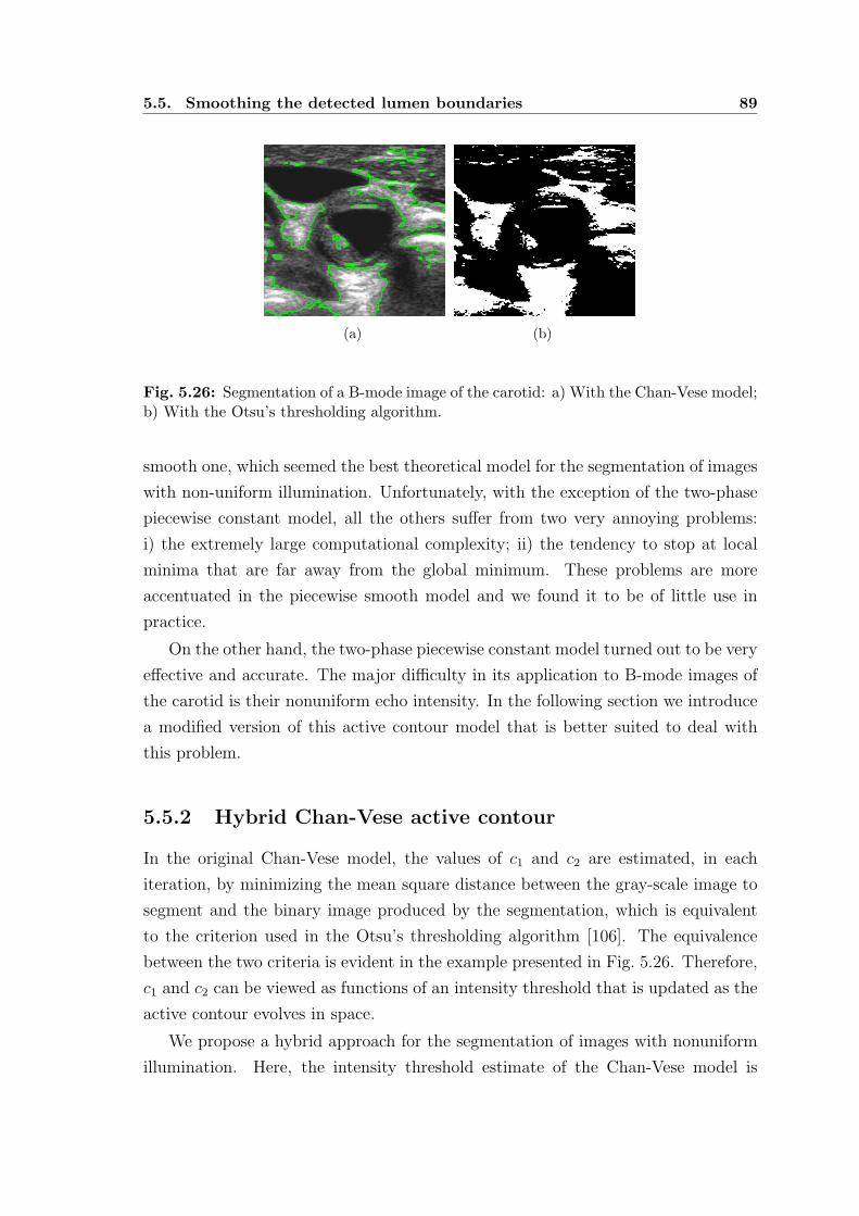
5.5. Smoothing the detected lumen boundaries 89
(a) (b)
Fig. 5.26: Segmentation of a B-mode image of the carotid: a) With the Chan-Vese model;b) With the Otsu’s thresholding algorithm.
smooth one, which seemed the best theoretical model for the segmentation of images
with non-uniform illumination. Unfortunately, with the exception of the two-phase
piecewise constant model, all the others suffer from two very annoying problems:
i) the extremely large computational complexity; ii) the tendency to stop at local
minima that are far away from the global minimum. These problems are more
accentuated in the piecewise smooth model and we found it to be of little use in
practice.
On the other hand, the two-phase piecewise constant model turned out to be very
effective and accurate. The major difficulty in its application to B-mode images of
the carotid is their nonuniform echo intensity. In the following section we introduce
a modified version of this active contour model that is better suited to deal with
this problem.
5.5.2 Hybrid Chan-Vese active contour
In the original Chan-Vese model, the values of c1 and c2 are estimated, in each
iteration, by minimizing the mean square distance between the gray-scale image to
segment and the binary image produced by the segmentation, which is equivalent
to the criterion used in the Otsu’s thresholding algorithm [106]. The equivalence
between the two criteria is evident in the example presented in Fig. 5.26. Therefore,
c1 and c2 can be viewed as functions of an intensity threshold that is updated as the
active contour evolves in space.
We propose a hybrid approach for the segmentation of images with nonuniform
illumination. Here, the intensity threshold estimate of the Chan-Vese model is

90 Chapter 5. Segmentation of the carotid lumen in B-mode images
replaced by a thresholding surface, keeping the rest of its attractive properties.
Basically, the proposed hybrid algorithm consists of two image processing stages, in
the following order:
1. An optimal smooth thresholding surface, Topt(x, y), is computed from the in-
tensities found at the edges along the boundaries produced by the dynamic
programming algorithm. This is done only once, before the initialization of
the active contour, and using the algorithm described in subsection 5.3.10.
2. The image is then processed by a modified version of the Chan-Vese two-phase
piecewise constant active contour, for which the constants c1 and c2 are deter-
mined as functions of Topt(x, y), such that the intensity threshold is preserved
at each pixel.
In the hybrid model, we set c1(x, y) = 2Topt(x, y) and c2(x, y) = 0, to keep the
intensity threshold as the mean of c1 and c2. The active contour is not used to
estimate the intensity threshold. It just uses its elastic properties and the intensity
topology of the image to clean the noise, smooth contours, improve their position
accuracy and close small carotid wall gaps.
Next, we discuss some important details related to the implementation of our
hybrid model.
An attractive property of the hybrid model is its faster convergence, compared
to the original active contour model.
The implicit function, φ, in equation 5.30, is initialized as a signed distance
function for which the zero level sets are the curves produced by the dynamic pro-
gramming algorithm. Since these curves are already very close to the real lumen
boundaries, a large number of iterations is saved.
To further reduce the computational effort, the processing is limited to the small-
est rectangular box containing the wall contour. An extra pair of lines is added to
the top and bottom of this box and an extra pair of columns is added to its sides,
in order to keep the wall contour away from the boundaries of the box. This will
insure the active contour will stay a closed curve, which might not happen if the
lumen region touched the boundaries of the box.
The Chan-Vese model spontaneously detects the interior of objects in an image.
While this is a blessing in most cases, it should be avoided in our case. Otherwise,
we may end up with more than the two regions we want, i.e., the lumen and the
rest of the image. This property disappears if φ becomes unable to generate new

5.5. Smoothing the detected lumen boundaries 91
(a) (b) (c)
Fig. 5.27: Inhibiting the detection of new holes in the hybrid Chan-Vese model: a) Initialactive contour; b) Segmentation result without inhibiting the detection of new holes insidethe carotid; c) Segmentation result inhibiting the detection of new holes.
isolated zero level sets. A fast and simple way to achieve this goal is to inhibit a
sign change in φ at any pixel for which there is no 8-neighbor with the same new
sign. In other words, φ is allowed to change sign only at pixels in the vicinity of the
active contour. An example of the effect introduced by this restriction is presented
in Fig. 5.27.
Since, at this time, we already know the location of the carotid wall, we restrain
the evolution of the active contour to the region delimited by the wall, inhibiting any
contour leakage at wall sections with weak echo or no echo at all. This restriction
is implemented by setting the intensities of the pixels outside the carotid to the
highest value of the image gray scale. Figure 5.28 shows an example of a contour
leakage through the carotid wall, which is stopped by the described restraint.
The active contour may also leak through the lumen boundary produced by the
dynamic programming algorithm, at places where boundary edges are missing. We
may reduce this risk by computing the thresholding surface under the restriction
of it dropping to zero at some reasonable distance, d, from the carotid. This gives
lower thresholds outside the detected lumen boundary, reducing the influence of
large values of the ICOV. Other possibilities are: i) to apply a smoothing filter to
the intensity profile along the boundary produced by the dynamic programming
algorithm; ii) to propagate to non-edge pixels of the contour the smallest intensity
at the closest edges pixels of the contour. In practice, the first solution seems to
give the best results. We usually set d = 3σd (the definition and estimation of σd
can be found in subsection 4.7.4 and section 4.9, respectively), to keep some safety
margin from the carotid wall. An example of the contour leakage through the lumen

92 Chapter 5. Segmentation of the carotid lumen in B-mode images
(a) (b) (c)
Fig. 5.28: Leakage of the active contour in the hybrid Chan-Vese model: a) Segmentationwith leakage through the carotid wall and through the lumen boundary, processing thewhole image; b) Segmentation restrained to the region inside the carotid wall; c) Groundtruth (green) and the automatic segmentation (red) when we also force the thresholdingsurface to zero at a distance d = 3σd from the carotid.
boundary is presented in Fig. 5.28, where we can also see the improvement obtained
with the proposed additional processing. For comparison, the ground truth was
included in the last image. Figure 5.29 shows the thresholding surfaces with and
without the additional restriction.
Two other examples of the final contour obtained with the hybrid algorithm are
presented in Fig. 5.30. The second example shows the significant improvement in the
location of the lumen boundary near plaque concavities that could no be detected by
the dynamic programming algorithm (see also Fig. 5.25). In both cases, the ground
truth is also displayed.
5.6 Results
There are several parameters to be defined in the Chan-Vese two-phase piecewise
constant active contour. With the exception of parameter µ, which determines
the elastic strength of the contour, all the others were set as suggested in [97, 98].
Therefore, we set: λ1 = λ2 = 1, to give equal importance to both phases in the image;
∆x = ∆y = 1, where (∆x,∆y) represents the image grid size; the regularizing
parameter of the Heaviside and delta functions as ε = ∆x; and the time step as
∆t = 0.1∆x.
The semi-implicit numerical scheme proposed in [97, 98] (see appendix E) was
used for equation 5.30. This numerical scheme was iterated until the maximum

5.6. Results 93
(a) (b)
Fig. 5.29: Thresholding surfaces for the hybrid Chan-Vese model: a) Surface used inthe segmentation presented in Fig. 5.28 (a) and Fig. 5.28 (b); b) Surface used in thesegmentation presented in Fig. 5.28 (c).
(a) (b)
Fig. 5.30: Ground truth (green) and the lumen boundaries obtained with the hybridChan-Vese model (red): a) From the contours displayed in Fig. 5.22 (a); b) From thecontours displayed in Fig. 5.25 (e).

94 Chapter 5. Segmentation of the carotid lumen in B-mode images
distance covered by the active contour became less than 0.01∆x, between two con-
secutive iterations. In other words, iterations were terminated when the active
contour virtually stopped.
Parameter µ can also be seen as a scale parameter, in the sense that the size
of the smallest objects detected by the active contour is proportional to the value
of µ. So, we defined this parameter as a function of the scale of the segmented
lumen, measured by the length, L, of the lumen boundary produced by the dynamic
programming algorithm. In longitudinal sections, L is the perimeter of the region
delimited by the two estimated contours (one above and the other bellow the medial
axis), to better capture the scale of the lumen region. The scale parameter was set
as µ = ρL×2552, where ρ = 10−4 was empirically determined as a good compromise
between a satisfactory level of smoothing and the fidelity to the data. The factor
2552, also used in [97, 98], is necessary to keep unity consistence in the level set
equation, since the image intensities are represented in the range 0, . . . , 255.
Besides the results presented in Fig. 5.28 (c) and Fig. 5.30, several other examples
of successful and unsuccessful segmentations of the carotid lumen are presented in
appendices H and I. Next we present several statistics of the segmentation results,
computed for our set of images and using the manual segmentations as the ground
truth.
Figure 5.31 gives the boxes and whiskers for the maximum distance error, Derr,
and the relative area error, Aerr, defined in section 4.9. These statistics were com-
puted for the subset of images for which the wall was successfully segmented. As
expected, the errors in the detection of the lumen boundaries are often larger than
in the wall detection, due to the typical hypoechogenicity of the plaque. Of course,
larger plaques will give larger errors, in case of failure. In many cases, the whole
plaque or a significant part of it is only detectable with complementary informa-
tion, like power-Doppler imaging. The medical specialist seems to add some mental
model to the data in the image that allows him to infer the approximate location of
the lumen boundary from very poor and discontinued lumen boundaries.
The CPU statistics for the lumen segmentation are presented in Fig. 5.32.
Finally, Fig. 5.33 shows the lumen area error statistics for the segmentation
results obtained with thresholding. The maximum distance error was not computed
in this case because the detection of a single noisy pixel inside the lumen would
distort the results.

5.6. Results 95
Transversal Longitudinal0
2
4
6
Der
r (m
m)
(a)
Transversal Longitudinal0
10
20
30
40
Aer
r (%
)
(b)
Fig. 5.31: Error statistics for the lumen segmentation: a) Derr b) Aerr.
DP CV Total0
20
40
60
80
Tim
e (s
)
(a)
DP CV Total0
2
4
6
8
10
Tim
e (s
)
(b)
Fig. 5.32: CPU statistics for the dynamic programming (DP), the hybrid Chan-Veseactive contour (CV) and the total time spent in the lumen segmentation: a) Longitudinalsections; b) Transversal sections.
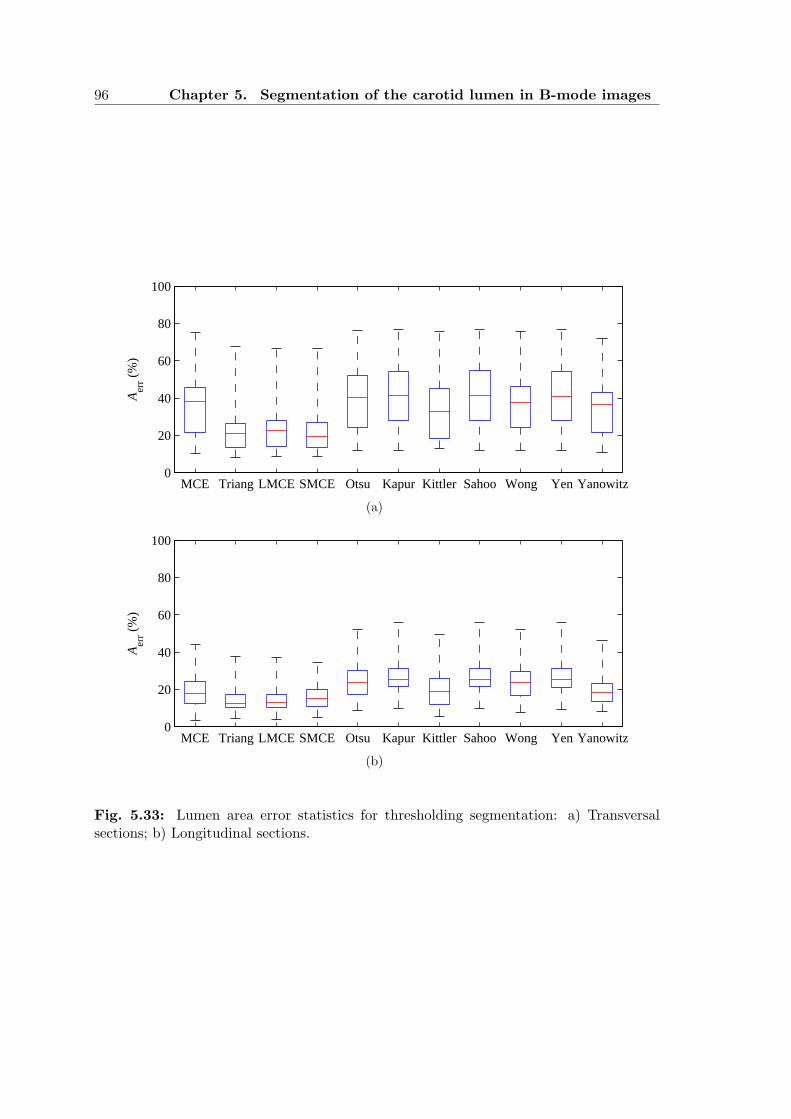
96 Chapter 5. Segmentation of the carotid lumen in B-mode images
MCE Triang LMCE SMCE Otsu Kapur Kittler Sahoo Wong Yen Yanowitz0
20
40
60
80
100
Aer
r (%
)
(a)
MCE Triang LMCE SMCE Otsu Kapur Kittler Sahoo Wong Yen Yanowitz0
20
40
60
80
100
Aer
r (%
)
(b)
Fig. 5.33: Lumen area error statistics for thresholding segmentation: a) Transversalsections; b) Longitudinal sections.

5.7. Concluding remarks 97
5.7 Concluding remarks
In thresholding segmentation, the triangle algorithm presented the best results. This
is the reason why we used it in chapter 4, to compute a quick rough estimate of the
lumen region. The LMCE algorithm was the second best thresholding algorithm.
Its results are very close to the triangle algorithm but it has the disadvantage of
requiring the knowledge of the wall location. As expected, the results get worse in
transversal sections, where the quality of the tissue boundaries is poorer. Unfor-
tunately, even the triangle algorithm failed to give reliable enough segmentations
when there is hypoechogenic plaque, significant noise inside the lumen or large echo
dropouts over the carotid region.
The proposed dynamic programming algorithm improved the lumen segmenta-
tion, but still presents significant errors when the echo along the boundary is too low
to produce any reasonable contour. The major drawback of this approach seems to
be the impossibility to capture deep concavities and sharp saliences, specially when
they are oriented in a direction similar to the direction of the boundary. Another
problem is the difficulty in integrating global constraints, like we did for the de-
tection of the carotid wall, which could help improving the poor response at very
degraded parts of the lumen boundary. Of course, if there is no signal at all, there
isn’t much we can do about it, considering it is not possible to use a shape prior.
Although the integration of a geometric term is attractive, the results show that
penalizing the length of the boundary may cause undesirable bypasses through the
interior of tissue regions. Penalizing the variation of the distance to the carotid wall
does not seem to work well either, since one can find plaques where this distance
varies a lot along the lumen surface. This motivated us to drop the geometric term
and do the smoothing in an independent step.
The combination of a smooth thresholding surface and the proposed modified
version of the Chan-Vese active contour proved to work well, both in the smoothing
and in the reduction of the errors in the location of the boundaries estimated by
the dynamic programming algorithm. The main disadvantages of this approach are
the computational effort and the risk of leakage of the active contour. If there are
no significant errors in the output of the dynamic programming algorithm, a simple
smoothing, with a weighted smoothing spline, should be enough, with the advantage
of being extremely fast to compute.
In spite of the good results for most of the images, the detection of the lumen
boundaries often fails in images with very poor quality, which are common in clinical

98 Chapter 5. Segmentation of the carotid lumen in B-mode images
practice. More studies should be pursued in order to reduce the gap between the
error rates in manual and automatic segmentations.

Chapter 6
RECONSTRUCTION OF THE
CAROTID 3D SURFACE
6.1 Introduction
Performing the segmentation of the carotid boundaries in 2D B-mode sections is con-
venient because they are more familiar to medical doctors, facilitating the validation
of the results and eventual corrections.
On the other hand, a 3D surface reconstruction of these boundaries has the
advantage of allowing other perspectives, through re-slicing of the data, that may
help to produce a better diagnosis.
One may take the best of both approaches by reconstructing the surfaces of the
carotid wall and of the lumen boundary directly from the segmented contours of a
sequence of B-scans of the artery. This procedure has several advantages relative
to alternatives based on data interpolation into voxels, as pointed out in chapter 2.
The validity of this approach was confirmed by a recent work [78], in which an ellipse
was used as a geometric model of the wall contour in each 2D transversal section of
the carotid. However, the authors of this work did all the segmentations by hand.
Some other relevant differences between their work and ours are: a) the approach
used to smooth the medial axis and the wall surface of the carotid; b) the treatment
of the lumen boundary after the wall smoothing; c) the algorithm used to obtain
new slices normal to the main axis.
The chapter starts with a brief overview of the approach, followed by several
sections which present and discuss, in detail, the algorithm proposed for the auto-
matic reconstruction of the 3D carotid surfaces, from a sequence of parallel transver-
sal slices of the CCA. The following sections introduce new algorithms for surface
reslicing in arbitrary directions and normal to the medial axis of the artery. Then,
some results and 3D measures of the carotid are presented. The chapter ends with

100 Chapter 6. Reconstruction of the carotid 3D surface
a section of concluding remarks.
6.2 Overview of the approach
Both the carotid wall surface and the lumen boundary surface are reconstructed.
The proposed algorithm starts by segmenting the carotid wall and the lumen
boundary contours in each B-mode image of the 3D volume, using the segmentation
algorithms proposed in chapters 4 and 5.
The segmented contours are resampled and the resulting set of points is used
to obtain a first estimate of the 3D surfaces, after matching the sampled points
between different frames.
Due to location errors of the volume slices, the obtained surfaces are rugged
and need to be smoothed, which is done with smoothing splines. First, a strong
smoothing is applied to the 3D curve that links the centroids of the carotid wall
contours. This step serves to align the segmented carotid wall contours and intro-
duces a significant improvement in the smoothness of the carotid wall surface, but
is not enough to produce the desired level of smoothness. Therefore, this surface is
subjected to a weaker additional smoothing. The displacements of the carotid wall
points, caused by the axis smoothing and wall surface smoothing, are transmitted,
through interpolation, to the points of the lumen surface. Finally, the lumen surface
also receives some very weak smoothing, which further improves the quality of the
surface without loosing a strong fidelity to the lumen data.
A fast and simple algorithm is introduced to reslice the reconstructed surfaces
in new positions and orientations. The problem of slicing a 3D surface consists in
determining the sliced 3D contour, defined as the intersection between an arbitrary
slicing plane and the surface to be sliced. Using a rigid geometric transformation
of the surface to be sliced, the problem can be viewed as the determination of the
zero level set of a 3D surface. This level set is a 2D contour, corresponding to the
projection of the sliced 3D contour in the slicing plane. The 3D contour can be
obtained from the determined level set, by inverting the geometric transformation
applied to the surface. But the level set may be enough for some applications, like
the computation of cross sectional areas.
The problem of reslicing in the direction normal to the medial axis of the carotid
wall is also addressed. In the proposed algorithm, the slice that passes through a
given 3D point and is normal to the medial axis is determined as the slice containing
that point and that minimizes the area inside the wall contour in the slice.

6.3. The freehand 3D volume 101
(a) (b)
Fig. 6.1: A 3D volume acquired with a 3D freehand system: a) Sequence of B-modeimages; b) A cut of the 3D volume.
6.3 The freehand 3D volume
The processed data consists of a sequence of parallel transversal slices, obtained
with a 3D freehand system and illustrated by the example in Fig. 6.1. This is the
usual form of the data for this kind of applications.
Longitudinal sections could also be included and used to improve the alignment
of the transversal sections. In fact, the integration of the longitudinal information
may be the best way to reduce the alignment errors between the segmented contours
of different transversal sections, specially for the lumen surface, where a strong
smoothing is out of the question.
In a more general approach, we could consider the acquisition of 2D slices with
arbitrary orientation. This approach introduces some undesired issues. First, the
ultrasound probe needs a 3D location tracker to estimate and save the 3D position
and orientation data of each image. The idea of connecting extra hardware to the
ultrasound machine is not very attractive since it disturbs the routine of the ex-
amination and causes extra difficulties to the medical doctor. Some probes come
with a built in 3D tracker and, with a proper ultrasound machine, can be used to
acquire 3D volumes. But the acquired data is protected by the manufacturer and it
is not available to export from the machine. Second, it is known that the quality of
the ultrasound image is related to the angle of incidence of the ultrasound beam at
the organ boundaries. A small angle will generally produce poorly defined bound-
aries, which would compromise the image segmentation results. In a modality like
ultrasound imaging, where the image quality is so low, this detail is very important.

102 Chapter 6. Reconstruction of the carotid 3D surface
That is why specialists prefer to acquire slices normal to the longitudinal axis of the
artery.
Besides the set of 2D images, another important complementary information for
the surface reconstruction is the voxel size, (∆x,∆y,∆z), which is frequently saved
in a separate text file.
Since our segmentation algorithm was conceived for the CCA, only this part of
the scanned artery was considered for 3D reconstruction.
6.4 Segmentation of the 3D volume
The segmentation of the volume is done sequentially, one 2D B-mode image at a
time, using the segmentation algorithms described in chapters 4 and 5.
The carotid boundaries segmented in each transversal section image are used to
initialize the segmentation of the next image in the sequence.
The segmentation algorithm starts by asking the user to click at a point near
the centroid of the lumen in the first frame of the 3D volume. This first estimate
is replaced, after the image segmentation, by the centroid of the detected lumen
boundary contour. The final estimate of the lumen centroid in each image is used
as the first estimate of the lumen centroid in the next frame of the volume sequence.
The RANSAC search during the segmentation of the wall, for all frames except
the first, is limited to a narrow band around the ellipse found for the previous frame.
In the first frame, a ROI around the lumen centroid is selected and segmented, as
described in chapter 4. This will considerably reduce the processing time. Figure 6.2
shows the segmented carotid wall contours for each frame of a 3D volume.
The segmented lumen boundary contour in each frame is saved in a file as a
chain of 2D coordinates, (x, y), before proceeding to the segmentation of the next
frame in the volume. The (x, y) coordinates are relative to the associated frame.
The parameters of the best ellipse fitted to the carotid wall are also saved, in an-
other file. These files may be used, afterwords, to compute the 3D surfaces of the
carotid boundaries. This clear separation between the segmentation and the surface
reconstruction is not only convenient but also desirable. In fact, the results of the
automatic segmentation may be used for other purposes, like the visualization and
eventual correction of the segmented boundaries. The surface rendering, based on
the set of previously segmented contours, is very fast, taking no more than one or
two seconds, making it adequate for real-time user interaction. The same cannot be
stated about the segmentation step, which is a heavy task, requiring at least three

6.5. Rendering of the 3D surfaces 103
Fig. 6.2: Segmented carotid wall contours of a 3D volume.
or four minutes to complete.
6.5 Rendering of the 3D surfaces
A 3D surface can be rendered using Matlab, with the function mesh(X,Y, Z). The
parameters X, Y and Z are m-by-n matrices, where m is the number of frames and
n− 1 is the number of points per frame. The x, y and z coordinates of the jth point
of the ith frame are saved in X(i, j), Y (i, j) and Z(i, j), respectively. To obtain a
cylindrical surface, the curves described by each line of X, Y and Z must be closed,
which means the first and the nth columns of these matrices must be equal. In other
words, a closed curve is represented by a polygon with N = n− 1 vertices.
The number of points per frame must be equal. Therefore, the segmented con-
tours in each B-scan must be re-sampled to obtain a constant number of points.
Fortunately, not all the points of the segmented contours are necessary to obtain a
good representation of the desired boundary surface. Usually, a sample of N = 50
points, equally spaced along the contour, is quite enough in practice.
The order sequence of the elements in matrices X, Y and Z determines the
connections between the corresponding 3D points. Each patch in the mesh is defined
by 4 vertices, with coordinates (X(i, j), Y (i, j), Z(i, j)), (X(i+1, j), Y (i+1, j), Z(i+
1, j)), (X(i, j + 1), Y (i, j + 1), Z(i, j + 1)) and (X(i+ 1, j + 1), Y (i+ 1, j + 1), Z(i+
1, j + 1)), such that 1 ≤ i ≤ m− 1 and 1 ≤ j ≤ n− 1.

104 Chapter 6. Reconstruction of the carotid 3D surface
x
y
(xc, yc)↑ ↑
Fig. 6.3: Matching points between ellipses: each ellipse is run in the counter-clockwisedirection and its starting position (red dot) is the positive intersection with the x axis,after translating the ellipse to the origin.
6.6 Matching points between consecutive curves
The sample of contour points in each frame must be well matched with the samples
of the adjacent frames, otherwise, the surface mesh will not be correctly built. In
the case of ellipses, the contour is represented by a set of 6 parameters. With
this information, it is easy to start the sampling at the same angle and choose the
same direction to walk along the ellipse. We chose to always start at the positive
intersection of the ellipse with the x axis, after translating it to the origin, and walk
in the counter-clockwise direction (or the clockwise direction, if the y axis is pointing
down). This is illustrated in Fig. 6.3.
At the output of the segmentation stage, each lumen boundary contour is de-
scribed by a sequence of points that are usually not well matched with the points
of the curves in adjacent frames. As shown in Fig. 6.4 (a), in some cases, these
curves may not even run in the same direction. To get a good matching between
the curve points of consecutive frames, the points in each frame may have to be
shifted backwards or forwards, along the corresponding line in matrices X, Y and
Z. Moreover, a curve also has to be flipped over if it does not run in the same
direction as the curve in the previous frame. Let δ = 1 represent a flipping of the
curve, δ = 0 represent no flipping, k ∈ 0, 1, ..., N − 1 the size of the shifting and
i ∈ 2, 3, ...,m the ith curve to match. Then, the optimum values of δ and k for
the ith curve are computed as
(δopti , kopt
i ) = arg minδ,k
d(i, δ, k) (6.1)

6.7. Alignment of the segmented carotid wall contours 105
↑↑
(a)
↑↑
(b)
Fig. 6.4: Matching points between contours of the lumen boundary: a) Sampled pointsin two consecutive frames, with starting positions and running directions indicated by thered dots and the arrows, respectively; b) Matching after the optimal shifting and flipping.
with
d(i, 0, k) =N
∑
j=1
‖pi−1,j − pi,((j−1+k) mod N)+1‖ (6.2)
d(i, 1, k) =N
∑
j=1
‖pi−1,j − pi,((N−j+k) mod N)+1‖ (6.3)
where N is the number of curve points per frame and pi,j is the 3D position of the
jth point of the ith curve.
Figure 6.4 (b) shows the curves of Fig. 6.4 (a), after matching their points ac-
cording to the above criterion.
6.7 Alignment of the segmented carotid wall
contours
When the image acquisition is made with a freehand 3D system, it is very difficult to
avoid some alignment errors between different frames of the 3D volume. Therefore,
the resulting surfaces will be far from smooth, as can be seen in Fig. 6.5 (a), for the
case of the carotid wall surface.
A good way of reducing this alignment error, as suggested in [78], is to fit a
weighted cubic smoothing spline [108], f(s), to the centroids of the segmented wall

106 Chapter 6. Reconstruction of the carotid 3D surface
(a) (b)
Fig. 6.5: Wall surface alignment: a) Wall surface obtained directly from the matchedsegmented 3D contours, without any alignment processing; b) Wall surface after alignmentwith our algorithm.
contours, by minimizing the following expression
p∑
i
wi (vi − f(si))2 + (1 − p)
∫ L
0
f ′′(s)2ds (6.4)
where: p is a real-valued smoothing parameter in the range 0 ≤ p ≤ 1; wi is the
weight of the ith centroid; vi represents the x, y or z component of the position
vector of the ith centroid; si is the value of the arc-length parameter, s ∈ [0, L],
at the ith centroid; and f ′′(s) is the second derivative of f with respect to s. The
value of p determines the balance between the smoothness of f and the fidelity to
the data. For p = 0, f is the least-squares straight line fit to the data. At the other
extreme, p = 1, f is the natural cubic spline interpolant.
The fitting can be made robust to outliers by using different weights for the
centroids. In [78], the weights were computed with a ’leave-one-out’ scheme. Each
weight is computed as wi = d−3i , where di is the Euclidean distance between the ith
centroid and the smooth spline obtained from all the other centroids, with uniform
weighting. When the weights for all the centroids are known, a final smooth spline
is computed using all the centroids and their estimated weights. This method has
two problems. First, it is computationally heavy, since the number of centroids is
usually large. Second, the distance function for each weight is chosen empirically.

6.8. Smoothing of the carotid wall surface 107
We use a more natural and faster method to determine the weighted smooth
cubic spline. In fact, it usually takes only a fraction of a second, in Matlab. We
take advantage of the tools of robust statistics described in chapter 4, in particular
the CMAD estimator and the Tukey’s function, presented in equations 4.2 and 4.4,
respectively. The estimation of the weighted smooth cubic spline, v = f(s), for each
coordinate, x, y and z, is summarized in the following steps:
1. Using equal weights and all the centroids, determine a smooth cubic spline,
f(s).
2. Compute the spline residuals, ri = vi − f(si).
3. Estimate the CMAD of the residuals. Since the median of the spline residuals
is zero, the expression simplifies to CMAD(r) = Cmed|r|.
4. Set the weight at each centroid as wi = g(ri;σ), where g(ri;σ) is the Tukey’s
function for a residual ri, with scale given by σ =√
5CMAD(r).
5. Using the new weights and all the centroids, determine a new smooth cubic
spline f ∗(s).
6. Compute the new spline residuals, r∗i = vi − f ∗(si).
7. If, for any centroid, | r∗
i−ri
r∗i
| > ε, where ε is a small positive threshold (ε = 1% is
quite enough), then make ri = r∗i and f = f ∗ and go back to step 3. Otherwise,
take the new spline as the weighted cubic spline estimate for the given data.
The smoothing parameter is set as
p =1
1 + h3
0.6
(6.5)
where h is the average spacing of the data sites, since this value of p is known to
give satisfactory smoothing1. Figure 6.5 (b) shows an example of the alignment
improvement achieved by our algorithm.
6.8 Smoothing of the carotid wall surface
From Fig. 6.5 (b), it is evident that, in spite of the significant reduction of the surface
irregularities, in general, the alignment of the centroids is not enough to produce
1 http://www.mathworks.com/access/helpdesk r13/help/toolbox/splines/csaps.html
108 Chapter 6. Reconstruction of the carotid 3D surface
the desired smooth carotid wall surface. In fact, this problem is difficult to elimi-
nate completely, without risking over-smoothing the data, in volumes acquired with
freehand systems. But the results may be further improved by a small additional
smoothing of the wall surface itself.
In [78], the smoothing of the carotid wall surface is done by fitting longitudinally
oriented smooth splines to matched points from adjacent cross-sectional carotid con-
tours. This has the disadvantage of smoothing only in the longitudinal direction.
Moreover, if the carotid bifurcation is also considered, an extra and specific treat-
ment is required for some of the points above the bifurcation.
It makes more sense to look for the smooth surface that best approximates the
complete set of 3D points. This way, the smoothing at each surface point takes into
consideration all the information from the point neighborhood, and not only the
information from the longitudinal direction. The general problem is quite complex,
involving both interpolation and approximation of sparse non-uniformly spaced 3D
data, and it may be solved with powerful but heavy tools, like the radial basis
function (RBF) interpolation [110]. But, in our case, we only consider the common
carotid artery, that has a simple cylindrical shape. Therefore, the surface smoothing
can be achieved with a generalization of equation 6.4. This solution is very fast
and produces very good results. It is used to compute a bi-variate tensor-product
smoothing spline for the matched and aligned (X,Y, Z) data of the carotid wall,
with uniform weighting.
The surface is represented as a parametric vector valued function, F (s, u) =
(X(s, u), Y (s, u), Z(s, u)), where s parameterizes the curve of the medial axis (that
passes through each centroid) and u parameterizes the curve in each frame, which,
ideally, should be perpendicular to the medial axis. Both parameters are normalized
to the range [0, 1].
Two smoothing parameters, ps and pu, have to be specified, one for each sur-
face parameter. Both of them fall in the range [0, 1] and both are computed as in
equation 6.5, by replacing h with the average spacing of the data sites in s and u,
respectively.
Along the u direction, the surface is closed and can be seen as a periodic function
of u. F (s, u) is computed over one period in the s direction and over three periods in
the u direction. Then, the middle period of the resulting smooth surface is selected.
This procedure reduces to virtually zero the discontinuities at the junction of the
tube along the direction of u. Figure 6.6 shows the surface presented in Fig. 6.5 (b)
after the additional smoothing produced by the algorithm just described.

6.9. Readjustment of the lumen position 109
Fig. 6.6: Carotid wall surface presented in Fig. 6.5 (b) after an additional smoothing ofthe surface itself.
6.9 Readjustment of the lumen position
Unlike the carotid wall surface, the lumen surface may present some irregularities
that are not caused by errors introduced by the freehand image acquisition system.
The plaque deposits may be responsible for some of these irregularities. Therefore, a
direct smoothing of the lumen surface is a risky step because one could be wiping off
important data and invalidating the diagnosis. But, the deformation of the carotid
wall, due to the smoothing of its surface and of the medial axis, must be transmitted
to the points of the lumen surface.
Since, at each frame, all the lumen points fall inside the region enclosed by the
carotid wall contour, the induced deformation of the lumen surface can be estimated
through interpolation. One may use 2D interpolation, in each frame, to estimate
each component of the 3D dislocation vector at each point of the lumen contour in
that frame.
To compute the interpolation, it is more convenient to view the 3D points of
the carotid boundaries as 2D points in the plane of the frame to which they belong.
From this perspective, the 3D dislocation vector, −→r j, for the jth curve point of a
frame is associated to a unique 2D point, Pj = (xj, yj), in that plane.
The interpolation problem for each frame can be posed as the computation of an
interpolation surface from a set of interpolating data located at points in the plane.
Three interpolating surfaces have to be computed in each frame, one for each of the

110 Chapter 6. Reconstruction of the carotid 3D surface
x, y and z components of the dislocation vectors.
The interpolation surface could be computed as a potential surface, as described
in subsection 5.3.10. But, in the present case, the points of the carotid wall and
lumen contours rarely coincide with image pixels. Therefore, the wall points have
to be approximated by the closest pixel, before computing the interpolation surface.
This introduces errors in the data, which are proportional to the size of the grid
step. Moreover, the dislocations at the lumen points have to be interpolated from
the values of the interpolation surface at the surrounding pixels. These problems
motivated the search for other solutions that are better tailored for the problem
in question. Two possible alternatives are the weighted average and the thin-plate
interpolation surfaces, which are discussed next.
6.9.1 Weighted average interpolation surface
An interpolation surface can be obtained as a weighted average of the interpolating
data. The value of the interpolation surface, f , at an interpolated point (xk, yk), is
given by
f(xk, yk) =
∑
j wk,jv(xj, yj)∑
j wk,j
(6.6)
where v(xj, yj) represents the interpolating data at the site Pj = (xj, yj) and
wk,j is the weight of the jth interpolating point when the data is interpolated at
Pk = (xk, yk). Each weight is computed as wk,j = 1/Φ(dk,j), where Φ(dk,j) is a
monotonically increasing function of the distance, dk,j, between points Pk and Pj,
and Φ(0) = 0.
This method is very simple and fast, since the data at the set of interpolated
points can be estimated without actually having to build an interpolation surface.
However, this approach has two important drawbacks: first, the choice of Φ is
arbitrary; second, the produced surface may not be very smooth, specially around
the interpolating points, as can be seen in the example of Fig. 6.7.
6.9.2 Thin-plate interpolation surface
A thin-plate smoothing spline2 can be used to build smooth interpolation surfaces
from data located at a set of sites in the plane. The thin-plate smoothing spline, f ,
2 http://www.mathworks.com/access/helpdesk r13/help/toolbox/splines/tpaps.html

6.9. Readjustment of the lumen position 111
Fig. 6.7: Weighted average interpolation surface, with Φ(d) = d2, for the set of interpo-lating points represented by the black dots.
is the unique minimizer of the weighted sum
p∑
j
[v(xj, yj) − f(xj, yj)]2 +
(1 − p)
∫
R2
[
f 2xx(x, y) + 2f 2
xy(x, y) + f 2yy(x, y)
]
dxdy
(6.7)
where: p is a real-valued smoothing parameter in the range 0 ≤ p ≤ 1; v(xj, yj) rep-
resents the x, y or z component of the dislocation vector, −→r j, at the jth interpolating
point, with coordinates (xj, yj); fxx, fxy and fyy are the second order derivatives of
f with respect to x and y. The value of p determines the balance between the error
of f , measured by the summation term, and the roughness measure given by the
integrand term. When p = 0, f is the least-squares approximation to the data by a
linear polynomial. When p = 1, f is the thin-plate spline interpolant to the data.
One may set p = 1 in the above equation and use it to estimate a very good
smooth interpolation surface, as the one presented in Fig. 6.8. The main disadvan-
tage of this method is that its computation time grows very fast with the number
of data points, since it involves the solution of a full linear system with as many
unknowns as there are data points. We found it to be a good solution as long as we
do not use much more than 50 points to represent the wall contours in each frame.
Otherwise, perhaps it is better to use potential surfaces with a small grid step.
Figure 6.9 shows the curves of the segmented carotid boundaries, in a frame of
a 3D volume, before and after the deformation caused by the smoothing operations.
As can be seen in this example, the smoothing operations may introduce an error
in the plaque area, which is corrected quite well by the interpolation step.

112 Chapter 6. Reconstruction of the carotid 3D surface
Fig. 6.8: Thin-plate interpolation surface, for the set of interpolating points representedby the black dots.
(a) (b) (c)
Fig. 6.9: Carotid wall (red) and lumen (blue) contours in a frame of a 3D volume:a) Before any smoothing; b) After smoothing the medial axis and the wall surface (thedashed curve is the original version); c) After interpolating the dislocation of the lumensurface (the dashed curves are the original versions).

6.9. Readjustment of the lumen position 113
(a) (b) (c)
Fig. 6.10: Example of a lumen surface: a) Obtained directly from the segmented lumencontours; b) After interpolating the deformation of the wall surface; c) After a lightsmoothing of the interpolated lumen surface.
In Fig. 6.10, one can see the lumen surfaces obtained from a 3D volume, before
and after the interpolation of the deformation induced by the smoothing of the
medial axis and the wall surface. Interpolating the deformation of the wall surface
does not necessarily produce a smoother lumen surface. In fact, as illustrated in
the example of Fig. 6.11, some sharp edges may even become sharper, resulting in
a more irregular surface at those regions.
The presence of plaque may introduce some irregularity in the lumen surface.
But most of the irregularities observed in the reconstructed lumen surface are caused
by location errors in the segmented lumen contours. The magnitude of these errors
tends to be larger when the plaque is hypoechogenic and large extensions of its
boundaries are missing. Although it is tempting to introduce additional smoothing
to the lumen surface, there is the risk of wiping off important details of the plaque.
This risk will be small if the level of smoothing is low. Figure 6.10 (c) shows the
result of applying, to the interpolated lumen surface, a smoothing similar to the one
used for the wall surface, but with a stronger fidelity to the data. Here, to make
sure the smoothed surface closely follows the data, the smoothing parameters are
computed as ps = 1/(1 + h3s/60) and pu = 1/(1 + h3
u/60), where hs and hu are the
average spacings of the lumen data sites in the direction of parameters s and u,
respectively3.
3 http://www.mathworks.com/access/helpdesk r13/help/toolbox/splines/csaps.html

114 Chapter 6. Reconstruction of the carotid 3D surface
Fig. 6.11: Interpolated lumen contour with sharp edges.
6.10 Surface slices
An important issue for the analysis of 3D volumes is the computation of arbitrary
slices. Most software in this field come with functions that compute slices of data
volumes in uniform grids. But, in our case, we need the intersection contour between
a specified slicing plane and a 3D surface. One could conceive and implement a
specific algorithm for this purpose. This is, perhaps, the ideal solution. A more
practical alternative is to take advantage of a general use algorithm that computes
level sets of a 3D surface. The idea is to apply a rigid geometric transformation
to the surface we want to slice, such that the slicing plane becomes coincident
with the x-y plane, and then compute the zero level set of the transformed surface.
To represent this level set in the original reference frame, the inverse geometric
transformation is applied. Although this is an indirect method, it is fast, relatively
simple to implement and works well in practice.
A slicing plane is completely defined by one of its points, P0 = (x0, y0, z0), and a
vector, −→n = (a, b, c), that is normal to the plane. Analogously, the x-y plane can be
defined by the point at the origin, (0, 0, 0), and a vector normal to that plane, like
the vector −→v = (0, 0, 1). The equation of the plane normal to vector −→n and passing
through point P0 is−→n · (P − P0) = 0 (6.8)
where P = (x, y, z) and the dot represents the inner product. From here, it is simple
to find the general equation of this plane, given by
ax+ by + cz + d = 0 (6.9)

6.10. Surface slices 115
with d = −(ax0 + by0 + cz0).
Any point, P = (x, y, z), of the slicing plane can be mapped into the x-y plane
through the following rigid body geometric transformation
P ′ = R(−→u , θ)(P − T ) (6.10)
where P ′ = (x′, y′, z′) is a point in the x-y plane, R(−→u , θ) is a 3D rotation matrix
and T is a translation vector. The direction about which to rotate is indicated by
vector −→u and θ is the angle of rotation.
Since the inverse of a rotation matrix is its transpose, the mapping from the x-y
plane back to the slicing plane can be computed as
P = RT (−→u , θ)P ′ + T (6.11)
where RT is the transpose of R.
The translation, T , of the slicing plane, relative to the x-y-z reference frame,
may be defined as the position vector of the intersection between the slicing plane
and the normal line passing through the origin. This definition leads to the following
equation for T (see appendix C)
T = − d
‖−→n ‖2−→n (6.12)
The rotation angle, θ, of the slicing plane is such that
cos(θ) =−→n · −→v
‖−→n ‖‖−→v ‖ (6.13)
which gives
θ = arccos
(
c
‖−→n ‖
)
(6.14)
In three dimensions, a rotation can be defined by a single angle of rotation, θ,
and the direction of the rotation axis specified by a unit vector, −→u = (α, β, γ). The
rotation matrix, R(−→u , θ), is
cos θ + α2(1 − cos θ) αβ(1 − cos θ) − γ sin θ αγ(1 − cos θ) + β sin θ
αβ(1 − cos θ) + γ sin θ cos θ + β2(1 − cos θ) βγ(1 − cos θ) − α sin θ
αγ(1 − cos θ) − β sin θ βγ(1 − cos θ) + α sin θ cos θ + γ2(1 − cos θ)
(6.15)

116 Chapter 6. Reconstruction of the carotid 3D surface
Fig. 6.12: The intersection of a slicing plane (in green) with a 3D surface (in red) is a3D contour, here represented by the curve in blue.
If θ = 0, the rotation matrix becomes the identity matrix and the direction of the
rotation axis has no importance. Otherwise, in our case, −→u is defined as
−→u =−→n ×−→v‖−→n ×−→v ‖ (6.16)
where −→n ×−→v is the cross product between vectors −→n and −→v .
Besides being fast and simple, another advantage of this approach is that the
2D points (x′, y′), whose coordinates are computed by equation 6.10, can be directly
used to compute some important measures, like lumen or plaque areas at any point
of the medial axis of the artery.
Figure 6.12 shows a 3D surface, an arbitrary slicing plane and the sliced contour
obtained with the procedure described above.
6.11 Slicing normal to the medial axis of the
artery
The analysis of the 3D surfaces reconstructed from the carotid boundaries helps to
get a better picture of the plaque distribution along the surface of the artery. It
aids to locate points with maximum degree of stenosis and allows the computation
of important measures like the area of the lumen or the area of the plaque along
the medial axis of the artery. But, to get good estimates of these measures, the
6.12. 3D measures 117
carotid surfaces have to be resliced at planes that are normal to the medial axis of
the artery.
The 3D smooth spline curve that links the aligned centroids of the carotid wall
is not a very good approximation of the real medial axis. It contains errors both in
the location of the axis and in the direction of its tangent vectors. Therefore, this
information should not be directly used to define the normal slicing planes, unless
the estimation of the medial axis is improved with a proper algorithm. This was the
approach followed in [78], where an iterative algorithm was used. At each iteration,
the local position, Q, and the tangential direction, −→e , of the medial axis are esti-
mated from the contour points of the current slice. Then, a new slice is obtained
a short distance away from point Q and normal to vector −→e . The local direction,−→e , is estimated as the mean of the unit vectors tangential to the wall surface, in
the longitudinal direction, at each of the contour points. The mean position of the
contour points gives the coordinates of point Q. An important drawback of this al-
gorithm is that the first slicing plane has to be chosen approximately perpendicular
to the carotid wall.
We think a better solution is to choose a point of the smooth spline curve that
links the centroids and to look for the orientation that minimizes the area inside
the contour in the slice that contains the given point. The search may start, for
instance, at the orientation of the vector tangent to the spline curve at the chosen
point. The initial surface will not, in general, be normal to the medial axis, but the
algorithm forces the slicing plane to converge to the normal orientation, where the
area is minimal for cylindrical surfaces. The fast Nelder-Mead simplex method [96]
was used to solve the minimization problem. Figure 6.13 shows an example with
the surface to be sliced, the chosen point of the slicing plane, the initial plane and
the plane found by the simplex method.
6.12 3D measures
There are several plaque measures that can be computed using normal reslicing of
the reconstructed 3D surfaces of the carotid. Some very interesting examples were
proposed in [78], in particular, the cross-sectional area or diameter of the lumen,
the volume of the plaque and the percentage stenosis index, SH , defined as
SH = 100 ×(
1 − Hlumen
Href
)
(6.17)

118 Chapter 6. Reconstruction of the carotid 3D surface
Fig. 6.13: Slicing normal to a 3D surface. The slicing plane has to contain a chosen pointof the smooth spline (black curve) that approximates the medial axis. The initial plane isin green and the blue plane gives the minimum area inside the sliced contour.
where Hlumen is some measurement of the lumen and Href is the corresponding ref-
erence measurement [78]. As suggested by the authors, these measurements may
be either the diameter, the area or the volume. In the case of the area, for in-
stance, Hlumen and Href are the areas inside the lumen and inside the carotid wall,
respectively.
The diameter measurements may not be realistic when the lumen is not con-
centric with the carotid wall. On the other hand, volume quantification gives a
single measure, with no information about the spatial distribution of the plaque.
Therefore, we did not consider these measurements.
Two very intuitive and informative measures are the plaque area and the stenosis
index for the area, computed as functions of the length of the medial axis. These
were the measurements adopted in this work.
6.13 Results
Using the proposed algorithms, the carotid wall and lumen surfaces were recon-
structed from the contours automatically segmented from two different 3D volumes.
The reconstructed surfaces are presented in Fig. 6.14 and Fig. 6.15, respectively.
For comparison, we also include, for each case, the surface obtained from a manual
segmentation of the same 3D volumes.
Plots of the area inside the carotid wall, the area inside the lumen and the
plaque area, as functions of the distance along the longitudinal direction, are given
in Fig. 6.16, Fig. 6.17 and Fig. 6.18, respectively. Similar plots of the area percentage

6.13. Results 119
(a) (b)
(c) (d)
Fig. 6.14: Reconstructed wall surfaces: a) Surface A, with automatic segmentation;b) Surface A, with manual segmentation; c) Surface B, with automatic segmentation;d) Surface B, with manual segmentation.

120 Chapter 6. Reconstruction of the carotid 3D surface
(a) (b)
(c) (d)
Fig. 6.15: Reconstructed lumen surfaces: a) Surface A, with automatic segmentation;b) Surface A, with manual segmentation; c) Surface B, with automatic segmentation;d) Surface B, with manual segmentation.

6.14. Concluding remarks 121
0 4 8 12 160
10
20
30
40
50
Length (mm)
Car
otid
Are
a (m
m2 )
(a)
0 10 20 30 400
20
40
60
80
100
Length (mm)
Car
otid
Are
a (m
m2 )
(b)
Fig. 6.16: Area inside the carotid wall, along the medial axis: a) For surface A, withautomatic (blue) and manual (red) segmentation; b) For surface B, with automatic (blue)and manual (red) segmentation.
stenosis index can be found in Fig. 6.19.
Finally, Fig. 6.20 and Fig. 6.21 present the relative area error, Aerr, defined in
section 4.9, for the carotid wall and lumen surfaces obtained from the automatic
segmentations. The surfaces obtained from the manual segmentations were used as
the ground truth.
6.14 Concluding remarks
The results presented in the previous section show that the algorithm proposed
for the carotid wall segmentation gives good estimates of the CCA wall surfaces.
Nevertheless, occasionally, some correction may be required from the expert.
The same conclusion cannot be taken for the lumen boundary. The main cause
for the large and frequent errors in the lumen segmentation is the severe hypoe-
chogenicity of the plaque in the exams. We remark that the manual segmentation
in these cases are usually supported by some parts of the lumen boundary that
are still perceivable, the rest of the curve being inferred as a smooth continuation
of these visible edges. It seems the user projects over the image a mental smooth
geometrical model that best fits the boundary cues that are visible. However, to
correctly locate these boundaries, even a specialist often needs to add the informa-
tion obtained through a power-Doppler image. More studies and new techniques
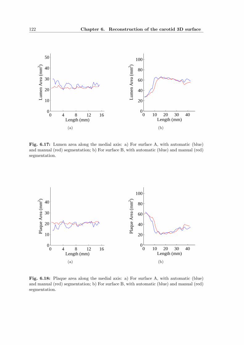
122 Chapter 6. Reconstruction of the carotid 3D surface
0 4 8 12 160
10
20
30
40
50
Length (mm)
Lum
en A
rea
(mm
2 )
(a)
0 10 20 30 400
20
40
60
80
100
Length (mm)
Lum
en A
rea
(mm
2 )(b)
Fig. 6.17: Lumen area along the medial axis: a) For surface A, with automatic (blue)and manual (red) segmentation; b) For surface B, with automatic (blue) and manual (red)segmentation.
0 4 8 12 160
10
20
30
40
Length (mm)
Pla
que
Are
a (m
m2 )
(a)
0 10 20 30 400
20
40
60
80
100
Length (mm)
Plaq
ue A
rea
(mm
2 )
(b)
Fig. 6.18: Plaque area along the medial axis: a) For surface A, with automatic (blue)and manual (red) segmentation; b) For surface B, with automatic (blue) and manual (red)segmentation.

6.14. Concluding remarks 123
0 4 8 12 160
20
40
60
80
Length (mm)
Are
a st
enos
is in
dex
(%)
(a)
0 10 20 30 400
20
40
60
80
Length (mm)
Are
a st
enos
is in
dex
(%)
(b)
Fig. 6.19: Area stenosis index along the medial axis: a) For surface A, with automatic(blue) and manual (red) segmentation; b) For surface B, with automatic (blue) and manual(red) segmentation.
0 15 30 45 600
10
20
30
40
50
Frame
Aer
r (%
)
(a)
0 10 20 300
10
20
30
40
50
Frame
Aer
r (%
)
(b)
Fig. 6.20: Relative area error for the carotid wall in each frame: a) For surface A; b) Forsurface B.
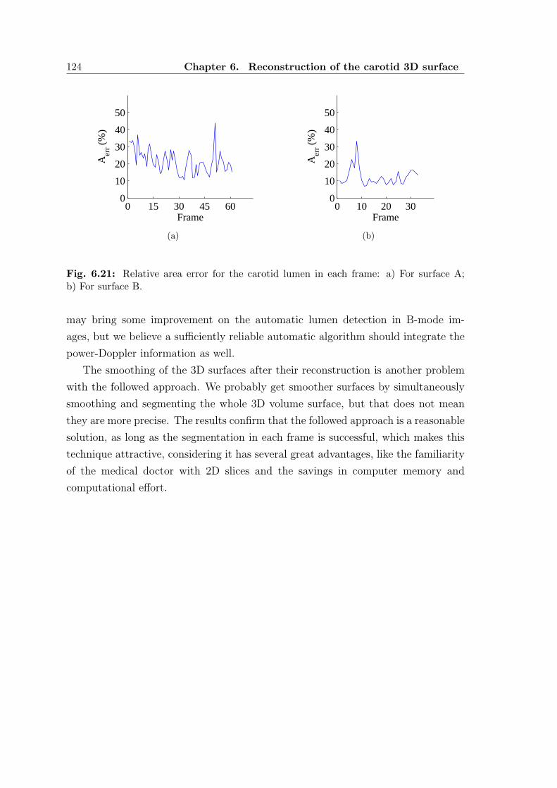
124 Chapter 6. Reconstruction of the carotid 3D surface
0 15 30 45 600
10
20
30
40
50
Frame
Aer
r (%
)
(a)
0 10 20 300
10
20
30
40
50
Frame
Aer
r (%
)
(b)
Fig. 6.21: Relative area error for the carotid lumen in each frame: a) For surface A;b) For surface B.
may bring some improvement on the automatic lumen detection in B-mode im-
ages, but we believe a sufficiently reliable automatic algorithm should integrate the
power-Doppler information as well.
The smoothing of the 3D surfaces after their reconstruction is another problem
with the followed approach. We probably get smoother surfaces by simultaneously
smoothing and segmenting the whole 3D volume surface, but that does not mean
they are more precise. The results confirm that the followed approach is a reasonable
solution, as long as the segmentation in each frame is successful, which makes this
technique attractive, considering it has several great advantages, like the familiarity
of the medical doctor with 2D slices and the savings in computer memory and
computational effort.

Chapter 7
CONCLUSIONS AND FUTURE
RESEARCH
A complete new approach was presented for the automatic detection of the common
carotid wall boundary, in B-mode images. The algorithm is based on a RANSAC
search of the best fit of a contour prior in the carotid image. It includes global
constraints, making it more powerful and robust to noise than other published ap-
proaches that use local constraints. A new non-linear smoothing filter for ultrasound
images was also proposed. This filter combines the ICOV edge detector with the
local intensity curvature, producing better preservation of important edges than
previously published filters.
An ICOV-based dynamic programming model was conceived for the detection
of the lumen boundary in longitudinal sections of the carotid, as well as its adap-
tation to transversal sections, where the boundary is a closed curve. The dynamic
programming approach was complemented with a new hybrid geometric active con-
tour, which uses a smooth thresholding surface and the image intensity topology
to: reduce some errors left by the dynamic programming segmentation; guide the
smoothing of the detected boundary.
The performance of the proposed segmentation algorithms was evaluated in a
large set of clinical B-mode images and compared to the manual tracings done by
an expert.
The algorithm conceived for the segmentation of the carotid wall proved to be
reliable in sections of the CCA. It can also detect the carotid wall in images that
include the carotid bulb and parts of the ICA, although, here, the success rate
decreases due to the higher complexity of the anatomy. Anyway, it seems some
additional information is missing in the segmentation model to avoid perturbations
caused by strong nearby tissue boundaries that do not belong to the carotid. These
constraints should, probably, be of anatomical and contextual nature. It isn’t clear,

126 Chapter 7. Conclusions and future research
however, which information to include and how to do it in an efficient manner. This
is an interesting and challenging subject for future studies.
The stiffness of the wall contour prior is a nice way to deal with heavy noise
and large wall gaps, but it also limits the ability of the prior to stick to the real
boundary at more irregular sections or when the shape of the real boundary deviates
too much from the prior model. Fortunately, the last situation is not frequent
and the errors involved are normally small. In any case, this limitation could be
reduced with a local refinement of the detected wall (e.g., with a ICOV-based active
contour), although, perhaps, at the expense of increasing the segmentation errors
at regions where the wall boundary is hardly visible or invisible. A more ambitious
approach would be to allow some sort of local geometric deformation of the contour
prior. But a practical implementation of this idea may not be compatible with the
RANSAC search. Due to all the specific difficulties of the carotid segmentation in
B-scans, the best segmentation approach is, perhaps, the registration of some sort
of discriminating image features with an atlas of the artery. This is probably the
way medical experts locate the boundaries of the artery in these images.
The results in the segmentation of the lumen boundary were not so good. There
are two main reasons for this. First, the possible presence of carotid plaques hin-
ders the introduction of a geometric prior of the lumen shape. Second, the hypoe-
chogenicity of most plaques often compromises their correct separation from the
lumen region. In this case, medical experts often need to analyze multiple B-scans
and color-coded duplex sonography to improve the detection. On the other hand,
the geometry of some plaque boundaries cannot be correctly detected by the consid-
ered dynamic programming algorithms, which are also not particularly suited to the
closed contours found in transversal sections of the carotid. Besides, a polar segmen-
tation scheme has always some dependence on the chosen seed point. Therefore, a
region-based segmentation of the lumen would be the ideal solution. But its viability
depends on the existence of B-mode image features that reliably discriminate the
lumen region from the plaque tissues and that can be used for segmentation. Un-
fortunately, such features do not seem to exist. Perhaps, the power-Doppler mode
images could be used as a complementary information to region-based segmentation.
Here is another interesting topic for future research.
New approaches were also proposed for the automatic reconstruction of 3D sur-
faces from the carotid boundaries, previously segmented in a sequence of B-mode
images acquired with a 3D ultrasound system. A level set algorithm was intro-
duced for the computation of new slices directly from the reconstructed 3D surfaces.

127
Finally, to obtain reliable estimates of surface slices normal to the carotid longitu-
dinal axis, a cross sectional area minimization approach was conceived. Examples
of 3D surfaces automatically reconstructed from sequences of B-scans, by the intro-
duced methods, were presented and compared to the surfaces obtained from manual
segmentations. Some clinically relevant measures were computed from the recon-
structed carotid surfaces.
The obtained results show that it is possible to compute good smooth 3D surfaces
directly from the carotid boundaries previously segmented in a set of 2D B-scans,
acquired with a freehand system. The proposed solution is very fast but is not di-
rectly applicable to bifurcations of the carotid. One possibility for future work would
be to adapt our algorithm to deal with the bifurcation. More powerful alternatives,
like the radial basis functions [110], are much heavier and more complex. But it
would be interesting to explore them as well.


Appendix A
ELLIPSE NORMAL
A conic section can be implicitly described as the zero level set of the following
function [95]
F (x, y) = ax2 + bxy + cy2 + dx+ ey + f (A.1)
where the values of the parameters a, b, c, d, e and f determine if the conic is an
ellipse (b2 − 4ac < 0), a parabola (b2 − 4ac = 0) or a hyperbola (b2 − 4ac > 0).
If b2 − 4ac < 0, then ac > 0, so a and c cannot be zero and must have the same
sign. Therefore, if a = 1, c is positive, as well as ∂2F/∂x2 = 2a and ∂2F/∂y2 = 2c.
Finally, (∂2F/∂x2)(∂2F/∂y2) − (∂2F/∂x∂y)2 = 4ac − b2 > 0, which means F (x, y)
is concave [111] and its gradient points outwards the zero level set.


Appendix B
RANSAC PROOF
If we take ω = ωp, the minimum number of samples of n points is given by
kp =(
1 +N√
1 − ωnp
)
/ωnp (B.1)
where ωnp is the probability of a good sample of n points. To simplify, let us assume
the number of edge points for each line segment is a constant, m. In this case,
P (’good point’/’good line segment’) = 1/m. If P (’good line segment’) = α, then
ωnp = (α/m)n and we may write
kp =(
1 +N√
1 − (α/m)n
)
/(α/m)n (B.2)
On the other hand, if we take ω = α, the minimum number of samples of n line
segments is
k∗s =(
1 +N√
1 − αn)
/αn (B.3)
and we have to evaluate mn samples of n points for each sample of n line segments.
Therefore, in this case, the minimum number of samples of n points will be
ks = mn(
1 +N√
1 − αn)
/αn (B.4)
It is easy to show that for m > 1 we always have ks < kp. Therefore, it is more
efficient to set ω = P (’good line segment’) and to evaluate all combinations of n
edge points for each sample of n line segments.


Appendix C
PLANE AND NORMAL LINE
The general equation of the plane passing through point P0 = (x0, y0, z0) and normal
to the vector −→n = (a, b, c) is
ax+ by + cz + d = 0 (C.1)
with d = −(ax0 + by0 + cz0).
The line passing through the origin of the x− y− z reference frame and normal
to the plane described above can be written in a parametric form as
(x, y, z) = λ(a, b, c) (C.2)
with λ ∈ R.
The intersection, Q, of this line with the above plane can be obtained by substi-
tuting x = λa, y = λb and z = λc in the general equation of the plane, giving
(
a2 + b2 + c2)
λ+ d = 0 ⇐⇒ λ = − d
‖−→n ‖2(C.3)
which means
Q = λ−→n = − d
‖−→n ‖2−→n . (C.4)


Appendix D
NUMERICAL SCHEME FOR THE
IMAGE FILTER
The following partial differential equation
∂I(x, y; t)
∂t= c(x, y; t)κ(x, y; t)‖∇I(x, y; t)‖ (D.1)
can be rewritten as
It = c‖∇I‖∇·( ∇I‖∇I‖
)
(D.2)
which is equivalent to
It = cI2xIyy − 2IxIyIxy + I2
yIxx
I2x + I2
y
(D.3)
Denoting the time step by ∆t and the image grid size by h, the last equation
can be discretized with the following explicit numerical scheme [85]
In+1i,j − In
i,j
∆t= cni,j
(DxIni,j)
2DyyIni,j − 2DxI
ni,jDyI
ni,jDxyI
ni,j + (DyI
ni,j)
2DxxIni,j
(DxIni,j)
2 + (DyIni,j)
2(D.4)
where
DxIni,j =
Ini+1,j − In
i−1,j
2h
DyIni,j =
Ini,j+1 − In
i,j−1
2h
DxxIni,j =
Ini+1,j − 2In
i,j + Ini−1,j
h2
DyyIni,j =
Ini,j+1 − 2In
i,j + Ini,j−1
h2
DxyIni,j =
Ini+1,j+1 − In
i−1,j+1 − Ini+1,j−1 + In
i−1,j−1
4h2

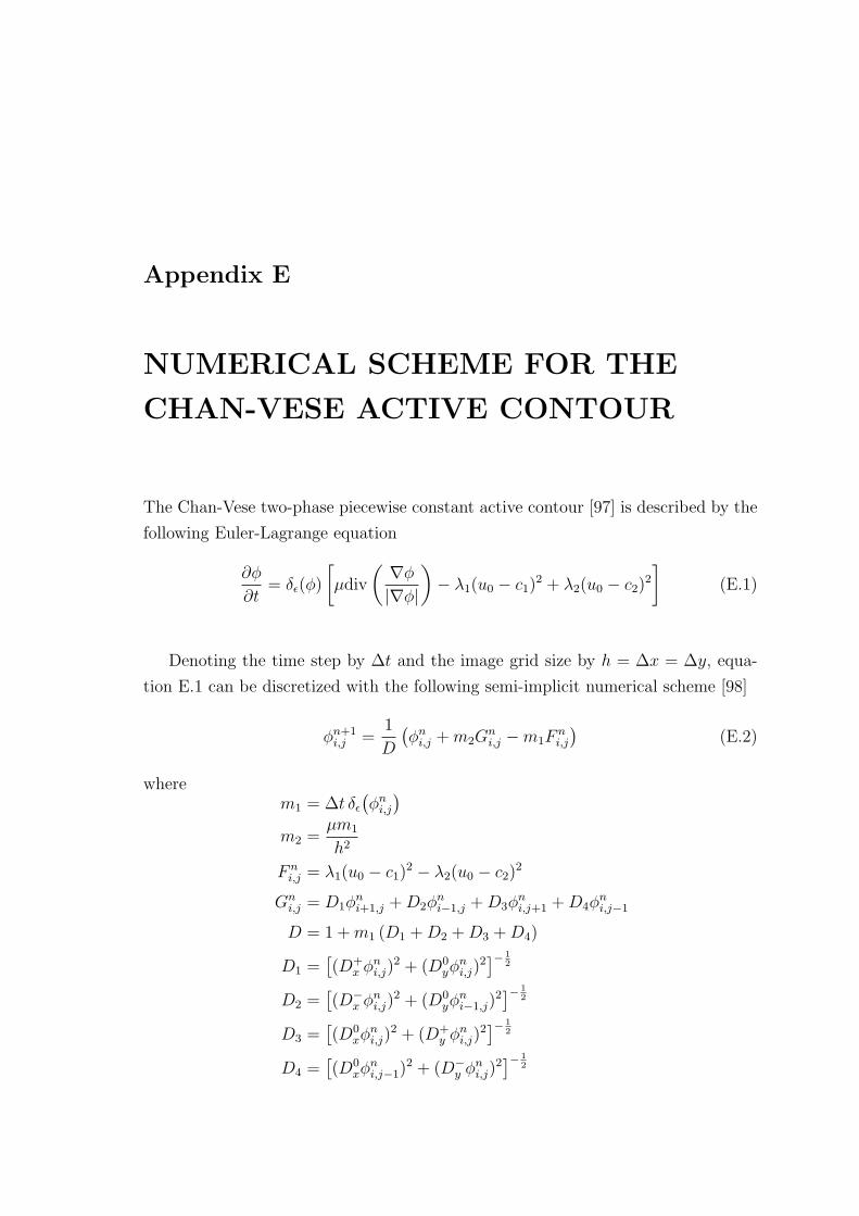
Appendix E
NUMERICAL SCHEME FOR THE
CHAN-VESE ACTIVE CONTOUR
The Chan-Vese two-phase piecewise constant active contour [97] is described by the
following Euler-Lagrange equation
∂φ
∂t= δε(φ)
[
µdiv
( ∇φ|∇φ|
)
− λ1(u0 − c1)2 + λ2(u0 − c2)
2
]
(E.1)
Denoting the time step by ∆t and the image grid size by h = ∆x = ∆y, equa-
tion E.1 can be discretized with the following semi-implicit numerical scheme [98]
φn+1i,j =
1
D
(
φni,j +m2G
ni,j −m1F
ni,j
)
(E.2)
wherem1 = ∆t δε
(
φni,j
)
m2 =µm1
h2
F ni,j = λ1(u0 − c1)
2 − λ2(u0 − c2)2
Gni,j = D1φ
ni+1,j +D2φ
ni−1,j +D3φ
ni,j+1 +D4φ
ni,j−1
D = 1 +m1 (D1 +D2 +D3 +D4)
D1 =[
(D+x φ
ni,j)
2 + (D0yφ
ni,j)
2]− 1
2
D2 =[
(D−x φ
ni,j)
2 + (D0yφ
ni−1,j)
2]− 1
2
D3 =[
(D0xφ
ni,j)
2 + (D+y φ
ni,j)
2]− 1
2
D4 =[
(D0xφ
ni,j−1)
2 + (D−y φ
ni,j)
2]− 1
2

138 Appendix E. Numerical scheme for the Chan-Vese active contour
D−x φ
ni,j =
φni,j − φn
i−1,j
h
D−y φ
ni,j =
φni,j − φn
i,j−1
h
D0xφ
ni,j =
φni+1,j − φn
i−1,j
2h
D0yφ
ni,j =
φni,j+1 − φn
i,j−1
2h
D+x φ
ni,j =
φni+1,j − φn
i,j
h
D+y φ
ni,j =
φni,j+1 − φn
i,j
h
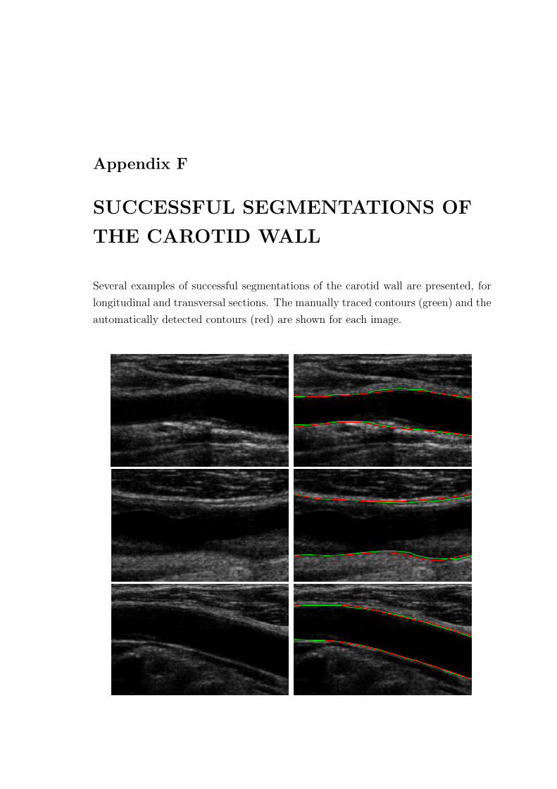
Appendix F
SUCCESSFUL SEGMENTATIONS OF
THE CAROTID WALL
Several examples of successful segmentations of the carotid wall are presented, for
longitudinal and transversal sections. The manually traced contours (green) and the
automatically detected contours (red) are shown for each image.

140 Appendix F. Successful segmentations of the carotid wall

141


Appendix G
UNSUCCESSFUL SEGMENTATIONS
OF THE CAROTID WALL
Several examples of unsuccessful segmentations of the carotid wall are presented,
for longitudinal and transversal sections. The manually traced contours (green) and
the automatically detected contours (red) are shown for each image.

144 Appendix G. Unsuccessful segmentations of the carotid wall

Appendix H
SUCCESSFUL SEGMENTATIONS OF
THE CAROTID LUMEN
Several examples of successful segmentations of the carotid lumen are presented, for
longitudinal and transversal sections. The manually traced contours (green) and the
automatically detected contours (red) are shown for each image.

146 Appendix H. Successful segmentations of the carotid lumen

147


Appendix I
UNSUCCESSFUL SEGMENTATIONS
OF THE CAROTID LUMEN
Several examples of unsuccessful segmentations of the carotid lumen are presented,
for longitudinal and transversal sections. The manually traced contours (green) and
the automatically detected contours (red) are shown for each image.

150 Appendix I. Unsuccessful segmentations of the carotid lumen

151

BIBLIOGRAPHY
[1] D. O’Leary, J. Polak, R. Kronmal, T. Manolio, G. Burke, and S. W. Jr.,
“Carotid-artery intima and media thickness as a risk factor for myocardial
infarction and stroke in older adults,” New Engl. J. Med., vol. 340, pp. 14–22,
1999.
[2] H. Hodis, W. Mack, L. LaBree, R. Selzer, C. Liu, C. Liu, and S. Azen, “The
role of carotid arterial intima-media thickness in predicting clinical coronary
events,” Ann. Intern. Med., vol. 128, pp. 262–9, February 1998.
[3] P. J. Touboul, P. Prati, P.-Y. Scarabin, V. Adrai, E. Thibout, and
P. Ducimetiere, “Use of monitoring software to improve the measurement of
carotid wall thickness by B-mode imaging,” J. Hypertension, vol. 10, no. 5,
pp. 37–41, 1992.
[4] J. Gariepy, M. Massonneau, J. Levenson, D. Heudes, A. Simon, and the
Groupe de Prevention Cardio-vasculaire en Medecine du Travail, “Evidence
for in vivo carotid and femoral wall thickness in human hypertension,” J.
Hypertension, vol. 22, no. 1, pp. 111–118, 1993.
[5] R. H. Selzer, H. N. Hodis, H. Kwong-Fu, W. J. Mack, P. L. Lee, C. R. Liu,
and C. H. Liu, “Evaluation of computerized edge tracking for quantifying
intima-media thickness of the common carotid artery from B-mode ultrasound
images,” Atherosclerosis, vol. 111, pp. 1–11, 1994.
[6] T. Gustavsson, Q. Liang, I. Wendelhag, and J. Wikstrand, “A dynamic pro-
gramming procedure for automated ultrasonic measurement of the carotid
artery,” Computers in Cardiology, pp. 297–300, 1994.
[7] R. J. Kozick, “Detecting interfaces on ultrasound images of the carotid artery
by dynamic programming,” SPIE, vol. 2666, pp. 233–241, 1996.

154 Bibliography
[8] Q. Liang, I. Wendelhag, J. Wikstrand, and T. Gustavsson, “A multiscale
dynamic programming procedure for boundary detection in ultrasound artery
images,” IEEE Trans. Med. Imag., vol. 19, no. 2, pp. 127–142, 2000.
[9] A. Schmidt-Trucksass, D. Cheng, M. Sandrock, J. Schulte-Monting, R. Raura-
maa, M. Huonker, and H. Burkhardt, “Computerized analysing system using
the active contour in ultrasound measurement of carotid artery intima-media
thickness,” Clinical Physiology, vol. 5, pp. 561–569, 2001.
[10] D. Cheng, A. Schmidt-Trucksass, K. Cheng, M. Sandrock, Q. Pu, and
H. Burkhardt, “Automatic detection of the intimal and the adventitial layers
of the common carotid artery wall in ultrasound B-mode images using snakes,”
in International Conference on Image Analysis and Processing, pp. 452–457,
B. Werner, 1999.
[11] D. Cheng, A. Schmidt-Trucksass, K. Cheng, and H. Burkhardt, “Using snakes
to detect the intimal and adventitial layers of the common carotid artery wall
in sonographic images,” Computer Methods and Programs in Biomedicine,
vol. 67, pp. 27–37, 2002.
[12] A. Gee, R. Prager, G. Treece, and L. Berman, “Engineering a freehand 3D
ultrasound system,” Pattern Recogn. Lett., vol. 24, no. 4-5, pp. 757–777, 2003.
[13] R. Rocha, A. Campilho, and J. Silva, “Segmentation of ultrasonic images of
the carotid,” in Int. Conf. Image Analysis and Recognition (ICIAR’2005),
Toronto, Canada, vol. 3656, pp. 949–957, Springer LNCS, September 2005.
[14] E. Bartels, Color-coded Duplex Ultrasonography of the Cerebral Vessels.
F.K.Schattauer,Germany, 1998.
[15] J. M. Thijssen, “Ultrasonic speckle formation, analysis and processing applied
to tissue characterization,” Pattern Recogn. Lett., vol. 24, no. 4-5, pp. 659–675,
2003.
[16] J. A. Noble and D. Boukerroui, “Ultrasound image segmentation: a survey,”
IEEE Trans. Med. Imag., vol. 25, no. 8, pp. 987–1010, 2006.
[17] J. Sanches, Reconstrucao 3D bayesiana a partir de sequencias ecograficas. PhD
thesis, Instituto Superior Tecnico, Lisboa, Marco 2003.

Bibliography 155
[18] M. Sonka, W. Liang, R. Stefancik, and A. Stolpen, Handbook of Medical Imag-
ing: Medical Image Processing and Analysis, vol. 2. SPIE, 2000.
[19] D. Baldassarre, M. Amato, A. Bondioli, C. R. Sirtori, and E. Tremoli, “Carotid
artery intima-media thickness measured by ultrasonography in normal clini-
cal practice correlates well with atherosclerosis risk factors,” Stroke, vol. 31,
pp. 2426 – 2430, October 2000.
[20] M. Halenka, “Noninvasive measurement of early atherosclerosis by high-
resolution B-mode ultrasonography,” Acta- Universitatis Palackianae Olomu-
censis Facultatis Medicae, vol. 142, pp. 7–12, 1999.
[21] S. Osher and J. A. Sethian, “Fronts propagating with curvature-dependent
speed: Algorithms based on Hamilton-Jacobi formulations,” Journal of Com-
putational Physics, vol. 79, pp. 12–49, 1988.
[22] J. A. Sethian, Level Set Methods and Fast Marching Methods. Cambridge
University Press, 1999.
[23] S. Osher and R. Fedkiw, Level Set Methods and Dynamic Implicit Surfaces.
Springer-Verlag. New York, 2003.
[24] J. Suri, S. Singh, S. Laxminarayan, X. Zeng, K. Liu, and L. Reden, “Shape
recovery algorithms using level sets in 2-D/3-D medical imagery: A state of
the art review,” IEEE Trans. Information Technology in Biomedicine, vol. 6,
pp. 8–28, March 2002.
[25] A. Tsai, A. J. Yezzi, W. M. W. III, C. Tempany, D. Tucker, A. Fan, W. E. L.
Grimson, and A. S. Willsky, “A shape-based approach to the segmentation of
medical imagery using level sets.,” IEEE Trans. Med. Imag., vol. 22, no. 2,
pp. 137–154, 2003.
[26] D. Cremers, T. Kohlberger, and C. Schnorr, “Nonlinear shape statistics in
Mumford-Shah based segmentation,” in Proc. European Conference on Com-
puter Vision (ECCV’2002), Copenhagen, vol. 2351, pp. 93–108, Springer
LNCS, 2002.
[27] D. Cremers, N. Sochen, and C. Schnorr, “Towards recognition-based varia-
tional segmentation using shape priors and dynamic labeling,” in Proc. Euro-
pean Conference on Computer Vision (ECCV’2003), vol. 2695, pp. 388–400,
Springer LNCS, 2003.
156 Bibliography
[28] D. Cremers, S. Osher, and S. Soatto, “Kernel density estimation and intrinsic
alignment for knowledge-driven segmentation: Teaching level sets to walk,”
Pattern Recognition, vol. 3175, pp. 36–44, 2004.
[29] J. G. Bosch, S. C. Mitchell, B. P. F. Lelieveldt, F. Nijland, O. Kamp, M. Sonka,
and J. H. C. Reiber, “Automatic segmentation of echocardiographic sequences
by active appearence motion models,” IEEE Trans. Med. Imag., vol. 21, no. 11,
pp. 1374–1383, 2002.
[30] M. Mignotte, J. Meunier, and J. C. Tardif, “Endocardial boundary estima-
tion and tracking in echocardiographic images using deformable template and
markov random fields,” Pattern Anal. Appl., vol. 4, no. 4, pp. 256–271, 2001.
[31] Y. Chen, H. Tagare, S. Thiruvenkadam, F. Huang, D. Wilson, K. S. Gopinath,
R. W. Briggs, and E. A. Geiser, “Using prior shapes in geometric active con-
tours in a variational framework,” Int. J. Comput. Vis., vol. 50, no. 3, pp. 315–
328, 2002.
[32] Y. Chen, F. Huang, H. D. Tagare, M. Rao, D. Wilson, and E. A. Geiser,
“Using prior shape and intensity profile in medical image segmentation,” in
IEEE Int. Conf. Comput. Vis., vol. 2, pp. 1117–1125, 2003.
[33] S. C. Mitchell, J. G. Bosch, B. P. F. Lelieveldt, R. J. van der Geest, J. H. C.
Reiber, and M. Sonka, “3-D active appearance models: segmentation of car-
diac MR and ultrasound images,” IEEE Trans. Med. Imag., vol. 21, no. 9,
pp. 1167–1178, 2002.
[34] L. X. Gong, S. D. Pathak, D. R. Haynor, P. S. Cho, and Y. Kim, “Paramet-
ric shape modeling using deformable superellipses for prostate segmentation,”
IEEE Trans. Med. Imag., vol. 23, no. 3, pp. 340–349, 2004.
[35] D. Shen, Y. Zhan, and C. Davatzikos, “Segmentation of prostate boundaries
from ultrasound images using statistical shape model,” IEEE Trans. Med.
Imag., vol. 22, no. 4, pp. 539–551, 2003.
[36] D. Shen, Z. Lao, J. Zeng, W. Zhang, I. A. Sesterhenn, L. Sun, J. W. Moul,
E. H. Herskovits, G. Fichtinger, and C. Davatzikos, “Optimized prostate
biopsy via a statistical atlas of cancer spatial distribution,” Med. Image Anal.,
vol. 8, pp. 139–150, 2004.
Bibliography 157
[37] J. Xie, Y. Jiang, and H. T. Tsui, “Segmentation of kidney from ultrasound
images based on texture and shape priors,” IEEE Trans. Med. Imag., vol. 24,
no. 1, pp. 45–57, 2005.
[38] N. Paragios, M. P. Jolly, M. Taron, and R. Ramaraj, “Active shape models
and segmentation of the left ventricle in echocardiography,” in Proc. Int. Conf.
Scale Space Theories PDEs Methods Computer Vision, vol. 3459, pp. 131–142,
2005.
[39] L. Fan, P. Santago, W. Riley, and D. M. Herrington, “An adaptive template-
matching method and its application to the boundary detection of brachial
artery ultrasound scans,” Ultrasound Med. Biol., vol. 27, no. 3, pp. 399–408,
2001.
[40] R. F. Wagner, S. W. Smith, J. M. Sandrik, and H. Lopez, “Statistics of speckle
in ultrasound B-scans,” IEEE Trans. Sonics Ultrson., vol. 30, no. 3, pp. 156–
163, 1983.
[41] C. B. Burckhardt, “Speckle in ultrasound B-scans,” IEEE Trans. Sonics Ul-
trason., vol. 25, no. 1, pp. 1–6, 1978.
[42] M. F. Insana, R. F. Wagner, B. S. Garra, D. G. Brown, and T. H. Shawker,
“Analysis of ultrasound image texture via generalized rician statistics,” Opt.
Eng., vol. 25, no. 6, pp. 743–748, 1986.
[43] P. M. Shankar, J. M. Reid, H. Ortega, C. W. Piccoli, and B. B. Goldberg,
“Use of non-Rayleigh statistics for the identification of tumors in ultrasonic
B-scans of the breast,” IEEE Trans. Med. Imag., vol. 12, no. 4, pp. 687–692,
1993.
[44] E. Jakeman, “K-distributed noise,” J. Opt. A: Pure Appl. Opt., vol. 1, pp. 784–
789, 1999.
[45] V. Dutt and J. F. Greenleaf, “Ultrasound echo envelope analysis using a homo-
dyned K-distribution signal model,” Ultrason. Imag., vol. 16, no. 4, pp. 265–
287, 1994.
[46] V. Dutt and J. F. Greenleaf, “Statistics of log-compressed echo envelope,” J.
Acoust. Soc. Amer., vol. 99, no. 6, pp. 3817–3825, 1996.

158 Bibliography
[47] L. Clifford, P. Fitzgerald, and D. James, “On the statistical characteristics
of log-compressed Rayleigh signals: Theoretical formulation and experimental
results,” J. Acoust. Soc. Amer., vol. 95, no. 3, pp. 1396–1400, 1994.
[48] A. Achim, A. Bezerianos, and P. Tsakalides, “Novel bayesian multiscale
method for speckle removal in medical ultrasound images,” IEEE Trans. Med.
Imag., vol. 20, no. 8, pp. 772–783, 2001.
[49] S. Gupta, R. C. Chauhan, and S. C. Sexana, “Wavelet-based statistical ap-
proach for speckle reduction in medical ultrasound images,” Med. Biol. Eng.
Comput., vol. 42, pp. 189–192, 2004.
[50] X. Zong, A. F. Laine, and E. A. Geiser, “Speckle reduction and contrast
enhancement of echocardiograms via multiscale nonlinear processing,” IEEE
Trans. Med. Imag., vol. 17, no. 4, pp. 532–540, 1998.
[51] Y. Yu and S. Acton, “Speckle reducing anisotropic diffusion,” IEEE Trans.
Image Processing, vol. 11, no. 11, pp. 1260–1270, 2002.
[52] Y. Yu and S. Acton, “Edge detection in ultrasound imagery using the instanta-
neous coefficient of variation,” IEEE Trans. Image Processing, vol. 13, no. 12,
pp. 1640–1655, 2004.
[53] C. Tauber, Filtrage anisotrope robuste et segmentation par B-spline snake:
application aux images echographiques. PhD thesis, Institut National Poly-
technique de Toulouse, Toulouse, Fevrier 2005.
[54] K. Z. Abd-Elmoniem, A. B. M. Youssef, and Y. M. Kadah, “Real time speckle
reduction and coherence enhancement in ultrasound imaging via non-linear
anisotropic diffusion,” IEEE Trans. Biomed. Eng., vol. 49, no. 9, pp. 997–
1014, 2002.
[55] P. M. Shankar, “A general statistical model for ultrasonic backscattering from
tissues,” IEEE Trans. Ultrason. Fer. Freq. Control, vol. 47, no. 3, pp. 727–736,
2000.
[56] P. M. Shankar, V. A. Dumane, J. M. Reid, V. Genis, T. George, F. Forsberg,
C. W. Piccoli, and B. B. Goldberg, “Use of K-distribution for classification of
breast masses,” Ultrasound Med. Biol., vol. 26, no. 9, pp. 1503–1510, 2000.

Bibliography 159
[57] L. Clifford, P. Fitzgerald, and D. James, “Non-Rayleigh first order statistics
of ultrasonic backscatter from normal myocardium,” Ultrasound Med. Biol.,
vol. 19, no. 6, pp. 487–495, 1993.
[58] P. M. Shankar, “Ultrasonic tissue characterization using a generalized Nak-
agami model,” IEEE Trans. Ultrason. Fer. Freq. Control, vol. 48, no. 6,
pp. 1716–1720, 2001.
[59] P. M. Shankar, V. A. Dumane, J. M. Reid, V. Genis, F. Forsberg, C. W.
Piccoli, and B. B. Goldberg, “Classification of ultrasonic B-mode images of
breast masses using Nakagami distribution,” IEEE Trans. Ultrason. Fer. Freq.
Control, vol. 48, no. 2, pp. 569–580, 2001.
[60] P. M. Shankar, V. A. Dumane, T. George, C. W. Piccoli, J. M. Reid, F. Fors-
berg, and B. B. Goldberg, “Classification of breast masses in ultrasonic B-
scans using Nakagami and K-distributions,” Phys. Med. Biol., vol. 48, no. 14,
pp. 2229–2240, 2003.
[61] P. M. Shankar, “The use of the compound probability density function in
ultrasonic tissue characterization,” Phys. Med. Biol., vol. 49, pp. 1007–1015,
2004.
[62] J. E. Wilhjelm, M. L. Gronholdt, B. Wiebe, S. K. Jespersen, L. K. Hansen,
and H. Sillesen, “Quantitative analysis of ultrasound B-mode images of carotid
atherosclerotic plaque: correlation with visual classification and histological
examination,” IEEE Trans. Med. Imag., vol. 17, pp. 910–922, December 1998.
[63] C. I. Christodoulou, C. S. Pattichis, M. Pantziaris, and A. Nicolaides, “Texture
based classification of atherosclerotic carotid plaques.,” IEEE Trans. Med.
Imag., vol. 22, no. 7, pp. 902–912, 2003.
[64] K. L. Chan, “Ultrasonic tissue characterization using fractal feature,” in IEE
Conf. Acoustic Sensing and Imaging, no. 369, pp. 183–188, 1993.
[65] D. Gabor, “Theory of communication,” J. of the Institute of Electical Engi-
neers, vol. 93, pp. 429–457, 1946.
[66] J. G. Daugman, “Uncertainty relation for resolution in space, spatial fre-
quency, and orientation optimized by twodimensional visual cortical filter,”
J. Opt. Soc. Am. A, vol. 2, no. 7, pp. 1160–1169, 1985.

160 Bibliography
[67] J. Canny, “A computational approach to edge detection,” IEEE Trans. Pat-
tern Analysis and Machine Intelligence, vol. 8, no. 6, pp. 679–698, 1986.
[68] T. Gustavsson, R. Abu-Gharbieh, G. Hamarneh, and Q. Liang, “Implementa-
tion and comparison of four different boundary detection algorithms for quan-
titative ultrasonic measurements of the human carotid artery,” Computers in
Cardiology, pp. 69–72, 1997.
[69] P. Detmer, G. Bashein, and R. Martin, “Matched filter identification of
left-ventricle endocardial borders in transesophageal echocardiograms,” IEEE
Trans. on Med. Imag., vol. 9, no. 4, pp. 396–404, 1990.
[70] M. Kass, A. Witkin, and D. Terzopoulos, “Snakes: Active contour models,”
International Journal of Computer Vision, pp. 321–331, 1988.
[71] A. R. Abdel-Dayem and M. R. El-Sakka, “Carotid artery contour extraction
from ultrasound images using multi-resolution analysis and watershed seg-
mentation scheme,” in Graphics, Vision and Image Processing (GVIP’2005),
Cairo, Egypt, December 2005.
[72] A. R. Abdel-Dayem and M. R. El-Sakka, “Carotid artery ultrasound image
segmentation using fuzzy region growing,” in Int. Conf. Image Analysis and
Recognition (ICIAR’2005), Toronto, Canada, vol. 3656, pp. 869–878, Springer
LNCS, September 2005.
[73] J. D. Gill, H. M. Ladak, D. A. Steinman, and A. Fenster, “Accuracy and vari-
ability assessment of a semiautomatic technique for segmentation of the carotid
arteries from three-dimensional ultrasound images,” Med. Phys., vol. 27, no. 6,
pp. 1333–1342, 2000.
[74] A. Zahalka and A. Fenster, “An automated segmentation method for three-
dimensional carotid ultrasound images,” Phys. Med. Biol., vol. 46, no. 4,
pp. 1321–1342, 2001.
[75] C. Baillard, C. Barillot, and P. Bouthemy, “Robust adaptive segmentation of
3D medical images with level sets,” tech. rep., IRISA, Campus Universitaire
de Beaulieu, France, 2000.
[76] G. Celeux and J. Diebolt, “L’algorithme SEM: un algorithme d’apprentissage
probabiliste pour la reconnaissance de melanges de densites,” Revue de statis-
tiques appliquees, vol. 34, no. 2, pp. 35–51, 1986.

Bibliography 161
[77] G. Celeux, D. Chauveau, and J. Diebolt, “On stochastic versions of the em al-
gorithm,” tech. rep., IRISA, Campus Universitaire de Beaulieu, France, 1995.
[78] D. Barratt, B. Ariff, K. Humphries, S. Thom, and A. Hughes, “Reconstruc-
tion and quantification of the carotid artery bifurcation from 3-D ultrasound
images,” IEEE Trans. Med. Imag., vol. 23, pp. 567–583, May 2004.
[79] J. C. Seabra, “Reconstrucao e diagnostico 3D ecografico da lesao
aterosclerotica,” Master’s thesis, Instituto Superior Tecnico, Lisboa, 2007.
[80] J. C. Seabra, J. Sanches, L. Pedro, and J. F. Fernandes, “Three-dimensional
ultrasonic assessment of atherosclerotic plaques,” in Iberian Conf. Patt. Recog-
nition and Image Analysis (IbPRIA’2007), June 2007.
[81] C. Xu and J. L. Prince, “Snakes, shapes, and gradient vector flow,” IEEE
Trans. Image Processing, vol. 7, no. 3, pp. 359–369, 1998.
[82] M. A. Fischler and R. C. Bolles, “Random sample consensus: a paradigm for
model fitting with applications to image analysis and automated cartography,”
Commun. ACM, vol. 24, no. 6, pp. 381–395, 1981.
[83] L. Rudin, S. Osher, and E. Fatemi, “Nonlinear total variation based noise
removal algorithms,” in Proceedings of the Eleventh Annual International
Conference of the Center for Nonlinear Studies on Experimental Mathemat-
ics: Computational Issues in Nonlinear Science, pp. 259–268, Elsevier North-
Holland, Inc., 1992.
[84] L. Rudin and S. Osher, “Total variation based image restoration with free
local constraints,” in Proceedings of IEEE International Conference on Image
Processing (ICIP’94), vol. 1, pp. 31–35, 1994.
[85] A. Marquina and S. Osher, “Explicit algorithms for a new time dependent
model based on level set motion for nonlinear deblurring and noise removal,”
SIAM J. Sci. Comput., vol. 22, no. 2, pp. 387–405, 2000.
[86] G. W. Zack, W. E. Rogers, and S. A. Latt, “Automatic measurement of sister
chromatid exchange frequency,” Journal of Histochemistry and Cytochemistry,
vol. 25, no. 7, pp. 741–753, 1977.
[87] D. Hearn and M. P. Baker, Computer Graphics. Prentice Hall, 1994.
162 Bibliography
[88] H. Breu, J. Gil, D. Kirkpatrick, and M. Werman, “Linear time Euclidean
distance transform algorithms,” IEEE Trans. Pattern Analysis and Machine
Intelligence, vol. 17, pp. 529–533, May 1995.
[89] P. Perona and J. Malik, “Scale-space and edge detection using anisotropic
diffusion,” IEEE Trans. Pattern Analysis and Machine Intelligence, vol. 12,
no. 7, pp. 629–639, 1990.
[90] M. J. Black, G. Sapiro, D. H. Marimont, and D. Heeger, “Robust anisotropic
diffusion,” IEEE Trans. Image Processing, vol. 7, no. 3, pp. 421–432, 1998.
[91] Z. Guo and R. W. Hall, “Parallel thinning with two-subiteration algorithms,”
Commun. ACM, vol. 32, no. 3, pp. 359–373, 1989.
[92] O. Chum, J. Matas, and J. Kittler, “Locally optimized RANSAC,” Lecture
Notes in Computer Science - Pattern Recognition, Springer Berlin/Heidelberg,
vol. 2781, pp. 236–243, 2003.
[93] D. A. Forsyth and J. Ponce, Computer Vision: A Modern Approach. Prentice
Hall, 2003.
[94] R. Burden and J. D. Faires, Numerical Analysis. Brooks Cole, 2000.
[95] A. Fitzgibbon, M. Pilu, and R. B. Fisher, “Direct least square fitting of el-
lipses,” IEEE Trans. Pattern Analysis and Machine Intelligence, vol. 21, no. 5,
pp. 476–480, 1999.
[96] G. Smirnov and V. Bushenkov, Curso de Optimizacao. Escolar Editora, 2005.
[97] T. Chan and L. Vese, “Active contours without edges,” IEEE Trans. Image
Processing, vol. 10, pp. 266–277, February 2001.
[98] L. A. Vese and T. F. Chan, “A multiphase level set framework for image
segmentation using the Mumford and Shah model,” Int. J. Comput. Vision,
vol. 50, no. 3, pp. 271–293, 2002.
[99] M. Sezgin and B. Sankur, “Survey over image thresholding techniques and
quantitative performance evaluation,” J. of Electronic Imaging, vol. 13, no. 1,
pp. 146–168, 2004.
[100] J. Kittler and J. Illingworth, “Minimum error thresholding,” Pattern Recog-
nition, vol. 19, no. 1, pp. 41–47, 1986.
Bibliography 163
[101] J. N. Kapur, P. K. Sahoo, and A. K. C. Wong, “A new method for gray-level
picture thresholding using the entropy of the histogram,” Comput. Vis. Graph.
Image Process, vol. 29, no. 3, pp. 273–285, 1985.
[102] P. Sahoo, C. Wilkins, and J. Yeager, “Threshold selection using Renyi’s en-
tropy,” Pattern Recogn., vol. 30, no. 1, pp. 71–84, 1997.
[103] J. C. Yen, F. J. Chang, and S. Chang, “A new criterion for automatic mutilevel
thresholding,” IEEE Trans. Image Processing, vol. 4, no. 3, pp. 370–378, 1995.
[104] N. Otsu, “A threshold selection method from gray-level histograms,” IEEE
Trans. Syst. Man Cybern., vol. 9, no. 1, pp. 62–66, 1979.
[105] S. D. Yanowitz and A. M. Bruckstein, “A new method for image segmenta-
tion,” Comput. Graph. Image Process., vol. 46, pp. 82–95, 1989.
[106] C. Li and C. Lee, “Minimum cross entropy thresholding,” Pattern Recogn.,
vol. 26, pp. 617–625, April 1993.
[107] C. Nicolini, A. M. Malvezzi, A. Tomaselli, D. Sposito, G. Tropiano, and E. Bor-
gogno, “DNASER I: Layout and data analysis,” IEEE Trans. Nanobioscience,
vol. 1, no. 2, pp. 67–72, 2002.
[108] C. de Boor, A Practical Guide to Splines. Springer-Verlag, 1978.
[109] D. Mumford and J. Shah, “Optimal approximations by piecewise smooth func-
tions and associated variational problems,” Communications on Pure and Ap-
plied Mathematics, vol. 42, no. 5, pp. 577–685, 1989.
[110] Y. Zhang, R. Rohling, and D. Pai, “Direct surface extraction from 3D freehand
ultrasound images,” in IEEE Visualization 2002, pp. 45–52, 2002.
[111] M. R. Spiegel and L. Abellanas, Formulas e Tabelas de Matematica Aplicada.
McGraw-Hill, 1990.