1

Optimal Segmentation of Signals Based on DynamicProgramming and Its Application to Image Denoising and

Edge Detection

Steven Kay and Xu Han

Abstract: An optimal procedure for segmenting one-dimensional signals whoseparameters are unknown and change at unknown times is presented. The method ismaximum likelihood segmentation, which is computed using dynamic programming. Inthis procedure, the number of segments of the signal need not be known a priori but isautomatically chosen by the Minimum Description Length rule. The signal is modeled asunknown DC levels and unknown jump instants with an example chosen to illustrate theprocedure. This procedure is applied to image denoising and edge detection. The resultsare compared with those obtained through classical procedures. The possible directionsfor improvement are discussed in the conclusion.

Keyword: Signal Segmentation, Dynamic Programming, Denoising, Edge Detection,MLE, MDL.

1 Introduction

Signal segmentation is a very important subproblem that appears in many problems such

as speech recognition, image feature extraction, edge detection, signal detection and

communications [1-6]. An example of segmentation of a time series is depicted in Figure

1. A data set { }[0], [1], , [ 1]x x x N −… is observed which is composed of SN segments of

differing statistics. With SN segments there are 1SN − transition times composing the set

{ }1 2 1, , ,SNn n n −… . Additionally, each segment may depend on a set of unknown parameters

è . The most general segmentation problem is to estimate the number of segments SN ,

the transition times in , and the unknown vector of parameters iè for each segment.

2

Figure 1 Segmentation problem.

There have been numerous attempts to solve the segmentation problem [7-9]. A

statistically optimal approach (for large data records) is to find the maximum likelihood

estimator (MLE) of the unknown parameters [10]. Unfortunately, due to the

computational burden of implementation which grows exponentially with the number of

segments, this has not been pursued. Suboptimal methods based on sequential estimation

have been proposed to reduce the computation. The disadvantage is the reduced

performance as well as the need for the setting of various thresholds. The choice of the

thresholds tends to be ad hoc and so reliable segmentation cannot always be obtained.

In this paper we propose an MLE segmenter whose computational complexity is

reduced drastically over a conventional implementation. This reduction is due to the use

of dynamic programming (DP) [11]. The approach which is proposed has been motivated

by the work of Bellman in fitting a piecewise linear model to a given curve [12]. Our

work was originally implemented for segmentation of autoregressive process in [19]. It

3

should also be mentioned that similar methods have been independently reported in [13]

and [20].

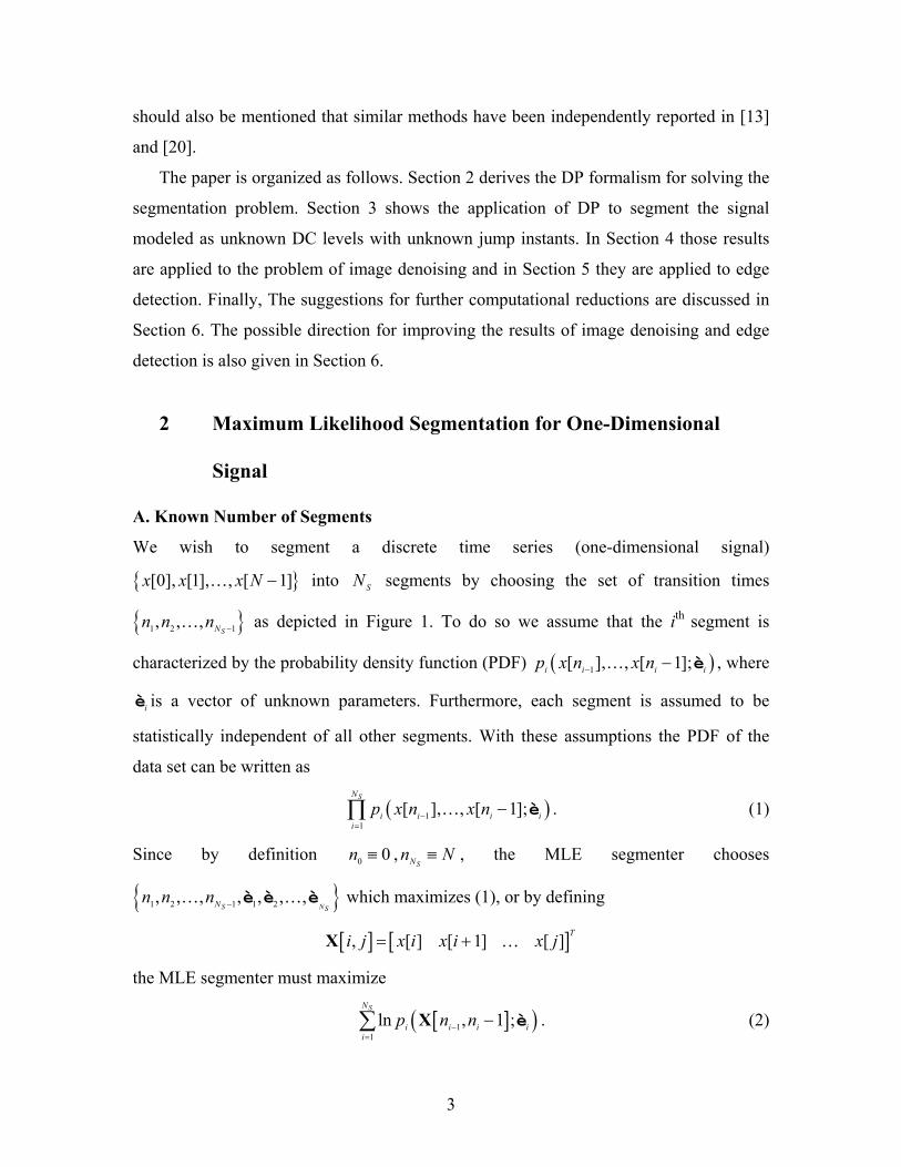
The paper is organized as follows. Section 2 derives the DP formalism for solving the

segmentation problem. Section 3 shows the application of DP to segment the signal

modeled as unknown DC levels with unknown jump instants. In Section 4 those results

are applied to the problem of image denoising and in Section 5 they are applied to edge

detection. Finally, The suggestions for further computational reductions are discussed in

Section 6. The possible direction for improving the results of image denoising and edge

detection is also given in Section 6.

2 Maximum Likelihood Segmentation for One-Dimensional

Signal

A. Known Number of Segments

We wish to segment a discrete time series (one-dimensional signal)

{ }[0], [1], , [ 1]x x x N −… into SN segments by choosing the set of transition times

{ }1 2 1, , ,SNn n n −… as depicted in Figure 1. To do so we assume that the ith segment is

characterized by the probability density function (PDF) ( )1[ ], , [ 1];i i i ip x n x n− − è… , where

iè is a vector of unknown parameters. Furthermore, each segment is assumed to be

statistically independent of all other segments. With these assumptions the PDF of the

data set can be written as

( )11

[ ], , [ 1];SN

i i i ii

p x n x n−=

−∏ è… . (1)

Since by definition 0 0n ≡ ,SNn N≡ , the MLE segmenter chooses

{ }1 2 1 1 2, , , , , , ,S NS

Nn n n − è è è… … which maximizes (1), or by defining

[ ] [ ], [ ] [ 1] [ ]T

i j x i x i x j= +X …

the MLE segmenter must maximize

[ ]( )11

ln , 1 ;SN

i i i ii

p n n−=

−∑ X è . (2)

4

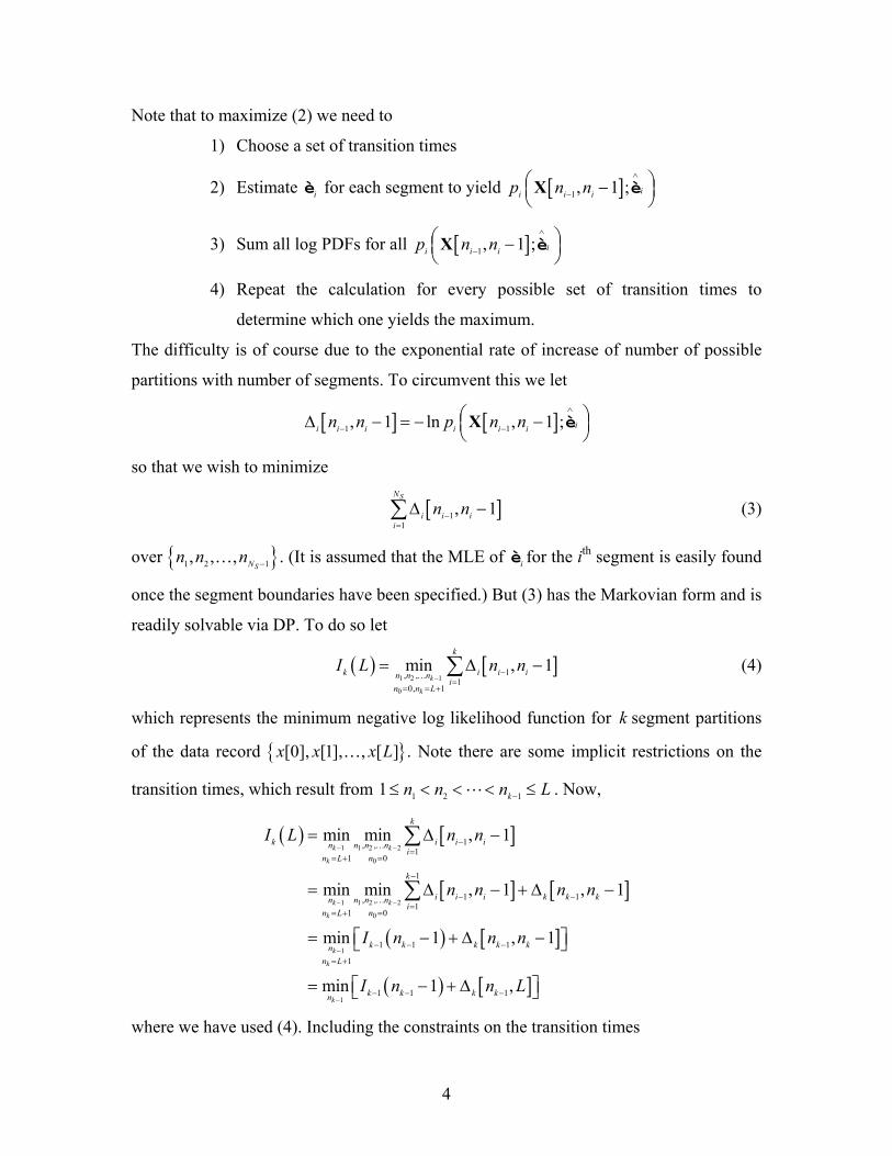
Note that to maximize (2) we need to

1) Choose a set of transition times

2) Estimate iè for each segment to yield [ ]1, 1 ; ii i ip n n∧

− −

X è

3) Sum all log PDFs for all [ ]1, 1 ; ii i ip n n∧

− −

X è

4) Repeat the calculation for every possible set of transition times to

determine which one yields the maximum.

The difficulty is of course due to the exponential rate of increase of number of possible

partitions with number of segments. To circumvent this we let

[ ] [ ]1 1, 1 ln , 1 ; ii i i i i in n p n n∧

− − ∆ − = − −

X è

so that we wish to minimize

[ ]11

, 1SN

i i ii

n n−=

∆ −∑ (3)

over { }1 2 1, , ,SNn n n −… . (It is assumed that the MLE of iè for the ith segment is easily found

once the segment boundaries have been specified.) But (3) has the Markovian form and is

readily solvable via DP. To do so let

( ) [ ]1 2 1

0

1, ,1

0, 1

min , 1k

k

k

k i i in n ni

n n L

I L n n−

−=

= = +

= ∆ −∑…(4)

which represents the minimum negative log likelihood function for k segment partitions

of the data record { }[0], [1], , [ ]x x x L… . Note there are some implicit restrictions on the

transition times, which result from 1 2 11 kn n n L−≤ < < < ≤ . Now,

( ) [ ]

[ ] [ ]

( ) [ ]

( ) [ ]

1 1 2 2

0

1 1 2 2

0

1

1

1, ,1

1 0

1

1 1, ,1

1 0

1 1 1

1

1 1 1

min min , 1

min min , 1 , 1

min 1 , 1

min 1 ,

k k

k

k k

k

k

k

k

k

k i i in n n ni

n L n

k

i i i k k kn n n ni

n L n

k k k k kn

n L

k k k kn

I L n n

n n n n

I n n n

I n n L

− −

− −

−

−

−=

= + =

−

− −=

= + =

− − −

= +

− − −

= ∆ −

= ∆ − + ∆ −

= − + ∆ −

= − + ∆

∑

∑

…

…

where we have used (4). Including the constraints on the transition times

5

( ) ( ) [ ]1

1 1 11min 1 ,

kk k k k kk n L

I L I n n L−

− − −− ≤ ≤= − + ∆ (5)

for 1, , , 1L k k N= − −… . The solution to our original problem occurs for Sk N= and

1L N= − . To begin the recursion we need to compute

( ) [ ] [ ]

[ ]1 1 0 1

11

, 0,

ln 0, ;

I L n L L

p L∧

= ∆ = ∆

= −

X è(6)

for 0,1, , 1L N= −… . The actual procedure embodied in (5) and (6) is as follows:

1) Compute (6) for 0,1, , 1L N= −… and store the results in ( )1I L . This is the

maximum likelihood for all data records from 0n = to n L= or for all the one-segment

“partitions”.

2) According to (5) the optimal two-segment partitions as a function of data record

length are found as

( ) ( ) [ ]1

2 1 1 2 11min 1 ,

n LI L I n n L

≤ ≤= − + ∆ .

To compute this we need to compute [ ]2 1,n L∆ for all 11 n L≤ ≤ (the lower limit is 1 to

allow for a minimum one sample first segment). To this we add ( )1 1 1I n − which has

already been found and stored in step 1.

3) We continue the procedure requiring at each step the computation of [ ]1,k kn L−∆ .

Hence the computation goes up linearly with number of segments.

It should also be noted that due to the recursive nature of the DP solution the best

2,3, , 1SN −… segmentations are found as a byproduct of the approach. This allows us to

determine the best segmentation when the number of segments is not known a priori as

described next.

B. Unknown Number of Segments

In order to determine the number of segments we employ the Minimum Description

Length (MDL) [14]. If we were naively to choose the partition as the one which

maximizes the likelihood, then we would always choose the maximum number of

segments. This is because more parameters (the iè ) are estimated as more segments are

assumed, causing the likelihood function to monotonically increase with number of

6

segments. The MDL as applied to our problem chooses the number of segments SN∧

as

the value of k which minimizes for 1,2, ,k S= …

( ) 1

1

MDL ln [ ], , [ 1]; ln2

kk

i i iii

rk p x n x n N

∧ ∧ ∧

−

=

= − − + ∏ è… . (7)

Here S is the maximum number of segments, which is chosen by the user.

{ }1 2 1 1 2, , , , , , ,k kn n n∧ ∧ ∧ ∧ ∧ ∧

− è è è… … is the MLE for the k -segment partition of the entire data

record. By definition 0 0n∧

= , SNn N∧

= . Finally, kr is the number of parameters estimated

for an assumed k segments. If the dimension of i

∧

è is iq , then

1

1k

k ii

r q k=

= + −∑ (8)

with the first term of (8) representing the estimated iè and the second due to the 1k −

transition times.

The first term of the MDL of (7) may be computed using DP as described in the

previous section. This is because the maximum likelihood solution using DP also

provides all the lower order solutions as well. Almost no extra computation is required

when the number of segments is unknown.

3 One-Dimensional Signal Modeling and Its Segmentation

We model the one-dimensional signal as a multilevel DC signal, which jumps at the

unknown transition times and is contaminated by white Gaussian noise (WGN). The

signal is

[ ]11

[ ] [ ] [ ]SN

i i ii

s n A u n u n−=

= −∑ (9)

where 0 1 2 10s sN Nn n n n n N−= < < < < < = and [ ]u n is the unit step sequence. Here N

is the length of the signal. The contaminated signal we observed is

[ ] [ ] [ ]x n s n w n= + (10)

where [ ]w n is WGN. Let [ ][0] [1] [ 1]T

x x x N= −X . The PDF of X is

7

( )( )

( )1

12

/ 2 221

1 1exp [ ]

22

S i

i

N n

N ii n n

p x n Aσπσ −

−

= =

= − − ∑ ∑X;A, n (11)

where 1 2[ ]s

T

NA A A=A , 1 2 1[ ]s

T

Nn n n −=n and 2σ is the variance of the

WGN. From Equation (11), the MLE of iA is

1

1

1

1[ ]

i

i

n

i

n ni i

A x nn n −

−∧

=−

=− ∑ . (12)

Then

[ ] [ ]

( )1

1 1

2121

2

, 1 ln , 1 ;

1[ ] ln 2

2 2

i

i

ii i i i i i

ni i

i

n n

n n p n n

n nx n A πσ

σ −

∧

− −

− ∧−

=

∆ − = − −

− = − + ∑

X è

(13)

Since ( )11

sN

i ii

n n N−=

− =∑ , we need only minimize

[ ]11

, 1S

N

i i ii

n n−=

∆ −∑ (14)

where [ ]1

21

1, 1 [ ]i

i

n

ii i in n

n n x n A−

− ∧

−=

∆ − = − ∑ . Comparing Equation (14) with Equation (4) and

(5), we know that we can use the method of DP to find ∧

A and ^

n which maximize

( )p X;A, n . Here, because the number of segments is unknown, we need to compute the

( )MDL k using Equation (7). Then the estimation of the number of segments, SN∧

is the

“valley” of value of k which globally minimizes the ( )MDL k over all possible segment

numbers.

In summary, assuming a minimum length of one sample, our DP algorithm applied to

segment one-dimensional signals is as follows:

1) Let 1k = , use Equation (6) to compute ( )1I L for 0,1, , 1L N= −… . Compute

( )MDL 1 according to Equation (7);

8

2) Use Equation (5) to sequentially compute the ( )mI L for 0,1, , 1L N= −…

based on the ( )1mI L− . Here 2m ≥ . Compute ( )MDL m according to Equation

(7). If ( ) ( )MDL MDL 1m m> − , stop the computation loop of Step 2 and let

1SN m∧

= − ;

3) Use a backward recursion to compute the estimates of the transition times.

Here we denote 1Valley( 1, ) kk L n −− , where 1kn − is the minimizing value of

( ) ( ) [ ]1

1 1 11min 1 ,

kk k k k kk n L

I L I n n L−

− − −− ≤ ≤= − + ∆ . Thus 1SN m

∧

= − , SNn N∧∧

≡ ,

1

2 1

1

0

Valley( 1, 1),

Valley( 2, 1),

Valley( , 1),

0

S

S S

N S

N S N

p p

n N N

n N n

n p n

n

∧

∧ ∧

∧ ∧

−

∧ ∧ ∧

− −

∧ ∧

+

∧

= − −

= − −

= −

≡

4) Compute the maximum likelihood estimate of each DC level iA as

1

1

1

1[ ]

i

i

n

i

i i n n

A x nn n

∧

∧−

−∧

∧ ∧

− =

=−

∑ .

It is important to notice that we use the local minimum of the MDL function as a

substitute for the global minimum in step 2. To make this algorithm realizable, this

approximation is necessary.

A computer simulation example is show in Figure 2. In this example, the multi-levels

of the original signal is T[1 4 2 6 -2 1 5 2]=A . The corresponding transition times

are T[20 50 65 100 105 110 115]=n . The DP estimate of the transition times is

T[20 50 65 100 105 110 115]∧

=n , and the MLE of the multi-levels is

T[1.1401 4.1335 1.4483 6.0351 -2.4869 0.8589 4.9438 2.3492]∧

=A . From

this experiment we find that DP estimation of the transition times is very accurate. The

MLE of the multiple DC levels differs from the true values to some extent due to the low

SNR. From Figure 2(d), we find that 8k = is a local minimum. This means that the use of

9

the local minimum instead of the global minimum in our DP algorithm produces good

results. Also, the estimation of the number of the segments is very accurate, even under

the condition of low SNR. It is important to notice another advantage of the algorithm. At

the end of the multiple DC level signal, the length of each DC level is just 5 samples.

However, the DP algorithm can still detect the transition times very precisely. This

motivates one to apply this algorithm to image denoising and edge detection.

(a) (b)

(c) (d)

Figure 2. Segmentation and reconstruction of one-dimensional multi-level signal. (Unknown number of

segments.

(a) Original multi-level DC signal;

(b) Observed signal contaminated by white Gaussian noise ( 2 1σ = );

(c) Reconstructed multi-level DC signal;

(d) Minimum Description Length of the segmentation.

10

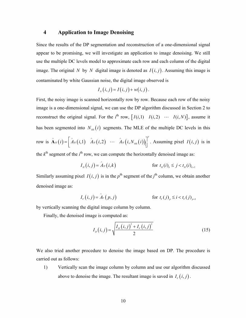
4 Application to Image Denoising

Since the results of the DP segmentation and reconstruction of a one-dimensional signal

appear to be promising, we will investigate an application to image denoising. We still

use the multiple DC levels model to approximate each row and each column of the digital

image. The original N by N digital image is denoted as ( ),I i j . Assuming this image is

contaminated by white Gaussian noise, the digital image observed is

( ) ( ) ( ), , ,NI i j I i j w i j= + .

First, the noisy image is scanned horizontally row by row. Because each row of the noisy

image is a one-dimensional signal, we can use the DP algorithm discussed in Section 2 to

reconstruct the original signal. For the ith row, [ ]( ,1) ( ,2) ( , )I i I i I i N , assume it

has been segmented into ( )HSN i segments. The MLE of the multiple DC levels in this

row is ( ) ( ) ( ) ( )( ),1 ,2 ,T

H H H H HSi A i A i A i N i∧ ∧ ∧ ∧ = A . Assuming pixel ( ),I i j is in

the kth segment of the ith row, we can compute the horizontally denoised image as:

( ) ( ), ,HHI i j A i k∧

= for 1( ) ( )H k H kt i j t i +≤ <

Similarly assuming pixel ( ),I i j is in the pth segment of the jth column, we obtain another

denoised image as:

( ) ( ), ,VVI i j A p j∧

= for 1( ) ( )V p V pt j i t j +≤ <

by vertically scanning the digital image column by column.

Finally, the denoised image is computed as:

( ) ( ) ( )2 2, ,

,2

H V

D

I i j I i jI i j

+= (15)

We also tried another procedure to denoise the image based on DP. The procedure is

carried out as follows:

1) Vertically scan the image column by column and use our algorithm discussed

above to denoise the image. The resultant image is saved in ( ),VI i j .

11

2) Horizontally scan image ( ),VI i j row by row and use the same algorithm to

denoise ( ),VI i j . The resultant image is saved in ( ),HVI i j .

We name this procedure as DP method I. And we name the previous procedure using

Equation (15) as DP method II. Computer simulation experiments show that the DP

method II is much better than DP method I in image denoising. We also compared the DP

method I and II with other classical image denoising algorithms such as low pass filtering

and median filtering. The simulation results indicate that DP method II is the best, both in

SNR and subjective evaluation. Here we compute the SNR as follows [15-16]:

2

1 1

210

1 1

( , )( ) 10log

( , ) ( , )

N N

i j

N N

i j

I i jSNR dB

I i j I i j

= =

∧

= =

=

−

∑∑

∑∑

where ( ),I i j is the original image and ( , )I i j∧

is the denoised image. Figure 3 shows the

results of different denoising methods. The original image is the standard 128 128× and

256 gray level peppers image. The variance of the white Gaussian noise is 400. Figure

3(c) is the denoised image obtained by low pass filtering. The 3 by 3 low pass filter is

defined as

1 1 11

1 1 19

1 1 1

=

H .

Figure 3(d) is the denoised image obtained by median filtering. The neighborhood of the

median filter is 3 by 3.

Using different variances for the WGN, we repeated this experiment based on the

same pepper image. The SNR of the denoised image by different methods is given in

Table 1. From the results shown in Figure 3 and Table 1, we see that the denoising results

of DP method II exceed those of the standard methods. The proposed method can

improve the SNR of the noisy image without blurring the image because the DP

segmentation algorithm is very accurate in estimating the transition positions. This is the

main advantage of the DP method II as compared with linear filtering or median filtering.

12

(a) (b)

(c) (d)

(e) (f)

Figure 3 The results of different denoising methods. (Variance of WGN is 400)(a) Original image 128 128× 256 gray level peppers image;

(b) Observed image contaminated by WGN ( 2σ =400), SNR= 16.34 dB;(c) Denoised image by low pass filtering, SNR= 17.34 dB;(d) Denoised image by median filtering, SNR= 18.78 dB;(e) Denoised image by DP method I SNR= 17.24 dB;(f) Denoised image by DP method II SNR= 19.69 dB;

13

2σ of WGN100 400 900

SNR (dB) of contaminatedimage

22.38 16.34 12.80

SNR (dB) of denoised imageBy low pass filtering

17.80 17.34 16.62

SNR (dB) of denoised imageBy median filtering

20.43 18.78 16.97

SNR (dB) of denoised imageBy DP method I

21.14 17.24 15.08

SNR (dB) of denoised imageBy DP method II

23.90 19.69 17.29

Table 1. The SNR of the denoised images.

In summary, DP method II is an excellent image denoising algorithm from the

standpoints of both SNR and subjective evaluation.

5 Application to Edge Detection

Noting the accuracy of the DP segmentation algorithm in estimating the transition

positions, we next apply it to edge detection. The details of its application to edge

detection are as follows:

1) Vertically scan the image column by column and apply the DP segmentation

algorithm to each column. Save the transition positions in a binary image ( , )BVI i j

defined as:

1 if is a transition position in the th column( , )

0 if is not a transition position in the th columnBV

i jI i j

i j

=

2) Horizontally scan the image row by row and apply the DP segmentation algorithm

to each row. Save the transition positions in a binary image ( , )BHI i j defined as:

1 if is a transition position in the th row( , )

0 if is not a transition position in the th rowBH

j iI i j

j i

=

3) Combine ( , )BVI i j and ( , )BHI i j to form a new binary image ( , )BEI i j . Then

( , )BEI i j is the result image of edge detection. ( , )BEI i j is defined as:

( , ) ( , ) ( , )BE BV BHI i j I i j I i j= +

14

where “+” means or.

Figure 4 shows the edge detection results of DP segmentation compared with the

results of the Canny and Prewitt operators. The original image is a 128× 128 ellipse

image contaminated by white Gaussian noise. The variance of the WGN is 900.

(a) (b)

(c) (d)

Figure 4 The edge detection results for ellipse image by various edge detection methods.

(a) The original image contaminated by WGN ( 2 900σ = )

(b) The result of Canny edge detection.

(c) The result of Prewitt edge detection.

(d) The result of DP edge detection.

Figure 5 shows the edge detection results by these methods for an 128× 128 irregular

polygon image contaminated by white Gaussian noise. The variance of the WGN is 900.

15

(a) (b)

(c) (d)

Figure 5 The edge detection results for irregular polygon image by various edge detection methods.

(e) The original image contaminated by WGN ( 2 900σ = )

(f) The result of Canny edge detection.

(g) The result of Prewitt edge detection.

(h) The result of DP edge detection.

From the results of Figure 4 and Figure 5, we determine that the DP segmentation is

more tolerant to noise as compared to the Canny edge detector. Also, the edges detected

by DP segmentation are thinner and smoother and have better continuity compared with

the ones detected by the Prewitt edge detector. Thus the DP segmentation is a very good

edge detector if the statistical model for the noise and the image is accurate.

16

6 Conclusion

Maximum likelihood segmentation appears to work quite well for one-dimensional

signals. The computational complexity of MLE segmentation, however, increases

exponentially with the increase of number of segments. When DP is used, the

computational complexity is substantially reduced, increasing only linearly with an

increased number of segments. The computational requirements can still be prohibitive

for a longer length signal. Other approaches such as parallel computing and hardware

implementation may therefore by necessary.

When applying DP segmentation to image denoising and edge detection, we should

have some a priori knowledge about the statistical model of the noise and the image. If

the images are very complicated, the multiple DC level model may not be suitable. The

autoregressive (AR) process, moving average (MA) process or other statistical models

may be necessary to represent the image [17-18]. MLE segmentation based on these

models can still be realized through DP [19].

17

Reference

[1] S. Kay, Fundamentals of Statistical Signal Processing, Volume 2: Detection Theory, Prentice-Hall, 1998.

[2] R. Haralick and L.G. Shapiro, “Survey: Image Segmentation,” Computer Vision, Graphics,Image Processing, 29:100-132, 1985

[3] E. Trucco and A. Verri, Introductory Techniques for 3-D Computer Vision, Prentice Hall, 1998.[4] L. R. Rabiner and R. W. Schafer, Digital Processing of Speech Signals, Prentice-Hall,

Englewood Cliffs, NJ, 1978.[5] M. Sonka, V. Hlavac, and R. Boyle, Image Processing, Analysis, and Machine Vision, Chapman

and Hall, 1993.[6] S. Haykin, Communication Systems: 4th Edition, John Wiley & Sons Inc., 2001.[7] M. Basseville and A. Benveniste, “Sequential Detection of Abrupt Changes in Spectral

Characteristics of Digital Signals,” IEEE Trans. in Info. Theory, Sept.1983, pp.709-724.[8] R. Andre-Obrecht, “A New Statistical Approach for the Automatic Segmentation of Continuous

Speech Signals,” IEEE Trans. on ASSP, vol.36, Jan. 1988, pp.29-40.[9] A.S. Willsky, “A Survey of Design Methods for Failure Detection in Dynamic Systems,”

Automatica, vol.12, 1976, pp.601-611.[10] S. Kay, Fundamentals of Statistical Signal Processing, Volume 1: Estimation Theory, Prentice-

Hall, 1993.[11] R. E. Larson and J. L. Castie, Principles of Dynamic Programming, vol. I, II, Marcel Dekker

Inc., NY, 1982.[12] R. Bellman and S. Dreyfus, Applied Dynamic Programming, Princeton Univ. Press, Princeton,

NJ, 1962.[13] N. Burobin, V. Mottl, and I. Muchnik, “An Algorithm of Detection of Multiple Change of

Properties of Random Process Based on the Dynamic Programming Method,” in Detection ofChange in Random Processes, Optimization Software Inc., NY, 1986.

[14] J. Rissanen, “Modeling by Shortest Data Description,” Automatica, vol. 14, 1978, pp.465-471.[15] W. K. Pratt, Digital Image Processing: PIKS Inside, Third Edition, Wiley-Interscience

Publication, 2001.[16] R. C. Gonzalez and P. Wintz, Digital Image Processing, Second Edition, Addison-Wesley,

Reading, Massachusetts, 1987.[17] S. Kay, Modern Spectral Estimation, Prentice-Hall, Englewood Cliffs, NJ, 1988[18] S. L. Marple, Jr., Digital spectral Analysis, Prentice-Hall, Englewood Cliffs, NJ, 1987.[19] S. Kay, “Optimal Segmentation of Time Series Based on Dynamic Programming,” Unpublished

notes, 1989[20] T. Svendsen and F. K. Soong, “On the Automatic Segmentation of Speech Signals,” in Proc.

Int. Conf. on Acoustics, Speech, and Signal Proc. (ICASSP), pp. 77-80, 1987.