image smoothing via l0 gradient minimizationkyros/courses/2530/papers/lecture-06/...image smoothing...
TRANSCRIPT
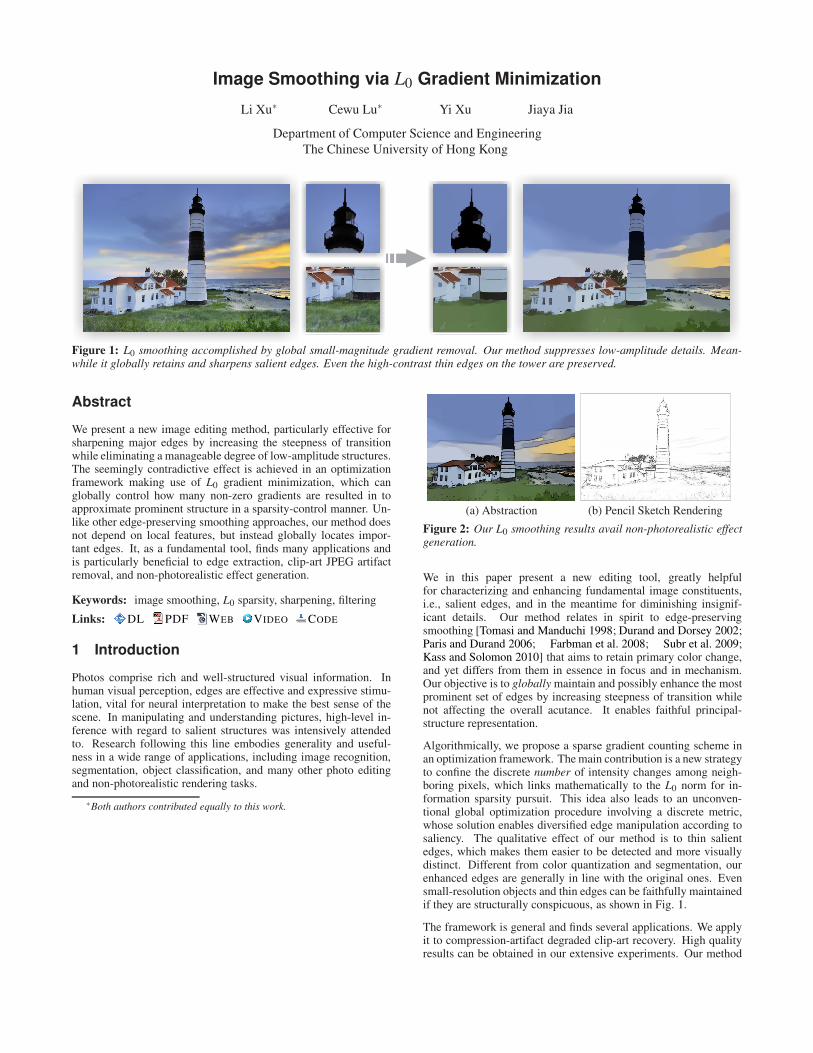
Image Smoothing via L0 Gradient Minimization
Li Xu∗ Cewu Lu∗ Yi Xu Jiaya Jia
Department of Computer Science and EngineeringThe Chinese University of Hong Kong
Figure 1: L0 smoothing accomplished by global small-magnitude gradient removal. Our method suppresses low-amplitude details. Mean-while it globally retains and sharpens salient edges. Even the high-contrast thin edges on the tower are preserved.
Abstract
We present a new image editing method, particularly effective forsharpening major edges by increasing the steepness of transitionwhile eliminating a manageable degree of low-amplitude structures.The seemingly contradictive effect is achieved in an optimizationframework making use of L0 gradient minimization, which canglobally control how many non-zero gradients are resulted in toapproximate prominent structure in a sparsity-control manner. Un-like other edge-preserving smoothing approaches, our method doesnot depend on local features, but instead globally locates impor-tant edges. It, as a fundamental tool, finds many applications andis particularly beneficial to edge extraction, clip-art JPEG artifactremoval, and non-photorealistic effect generation.
Keywords: image smoothing, L0 sparsity, sharpening, filtering
Links: DL PDF WEB VIDEO CODE
1 Introduction
Photos comprise rich and well-structured visual information. Inhuman visual perception, edges are effective and expressive stimu-lation, vital for neural interpretation to make the best sense of thescene. In manipulating and understanding pictures, high-level in-ference with regard to salient structures was intensively attendedto. Research following this line embodies generality and useful-ness in a wide range of applications, including image recognition,segmentation, object classification, and many other photo editingand non-photorealistic rendering tasks.
∗Both authors contributed equally to this work.
(a) Abstraction (b) Pencil Sketch Rendering
Figure 2: Our L0 smoothing results avail non-photorealistic effectgeneration.
We in this paper present a new editing tool, greatly helpfulfor characterizing and enhancing fundamental image constituents,i.e., salient edges, and in the meantime for diminishing insignif-icant details. Our method relates in spirit to edge-preservingsmoothing [Tomasi and Manduchi 1998; Durand and Dorsey 2002;Paris and Durand 2006; Farbman et al. 2008; Subr et al. 2009;Kass and Solomon 2010] that aims to retain primary color change,and yet differs from them in essence in focus and in mechanism.Our objective is to globally maintain and possibly enhance the mostprominent set of edges by increasing steepness of transition whilenot affecting the overall acutance. It enables faithful principal-structure representation.
Algorithmically, we propose a sparse gradient counting scheme inan optimization framework. The main contribution is a new strategyto confine the discrete number of intensity changes among neigh-boring pixels, which links mathematically to the L0 norm for in-formation sparsity pursuit. This idea also leads to an unconven-tional global optimization procedure involving a discrete metric,whose solution enables diversified edge manipulation according tosaliency. The qualitative effect of our method is to thin salientedges, which makes them easier to be detected and more visuallydistinct. Different from color quantization and segmentation, ourenhanced edges are generally in line with the original ones. Evensmall-resolution objects and thin edges can be faithfully maintainedif they are structurally conspicuous, as shown in Fig. 1.
The framework is general and finds several applications. We applyit to compression-artifact degraded clip-art recovery. High qualityresults can be obtained in our extensive experiments. Our method

(a) BLF [1998] (b) LCIS [1999] (c) WLS [2008] (d) Total Variation (TV) [1992] (e) Ours
Figure 3: Signal obtained from an image scanline, containing both details and sharp edges. (a) Result of bilateral filtering. (b) Result ofanisotropic diffusion used in the LCIS system. (c) Result of WLS optimization. (d) Result of TV smoothing. (e) Our L0 smoothing result.
can also profit edge extraction, a fundamentally important opera-tor, by effectively removing part of noise, unimportant details, andeven of slight blurriness, making the results immediately usable inimage abstraction and pencil sketch production, as shown in Fig.2. In traditional layer decomposition, with an additional step toavoid structure over-enhancement, our method is applicable to de-tail enhancement based on separating layers, and possibly to HDRtone mapping after parameter tuning. We show several examplesalong with discussion of limitations that our method might causeover-sharpening for large illumination variation spanning dozensof pixels when strong smoothing is applied.
2 Background and Motivation
Edge-preserving smoothing can be achieved by local filter-ing, including bilateral filtering [Tomasi and Manduchi 1998],its accelerated versions [Paris and Durand 2006; Weiss 2006;Chen et al. 2007] and relatives [Choudhury and Tumblin 2003;Fattal 2009; Baek and Jacobs 2010; Kass and Solomon 2010]. Ro-bust optimization-based approaches have also been advo-cated, represented by the weighted least square optimization[Farbman et al. 2008] and envelope extraction [Subr et al. 2009].We discuss their properties using the 1D signal example (a scan-line of a natural image) shown in Fig. 3.
Bilateral filtering is widely used for its simplicity and effective-ness in removing noise-like structures. This method trades off be-tween details flattening and sharp edge preservation, as discussed in[Farbman et al. 2008]. Its result is shown in Fig. 3(a). Anisotropicdiffusion [Perona and Malik 1990; Black et al. 1998] is also de-signed for suppressing noise while preserving important structures,which involves an edge-stopping function to prevent smoothingfrom crossing strong edges. The change of structures accumulatesand the output would converge to a constant-value image unlessbeing stopped halfway. One result is shown in Fig. 3(b).
Farbman et al. [2008] proposed a robust method with the weightedleast square (WLS) measure. The optimization framework withedge preserving regularization is more flexible compared with lo-cal filtering. Its result is shown in Fig. 3(c). Another type of edgepreserving regularization is total variation (TV) [Rudin et al. 1992],which is widely used to remove noise from images. It however alsopenalizes large gradient magnitudes, possibly influencing contrastduring smoothing. One example is shown in Fig. 3(d).
Subr et al. [2009] considered local signal extremes and usededge-aware interpolation [Levin et al. 2004; Lischinski et al. 2006]to compute envelopes. A smoothed mean layer is extracted by aver-aging the envelopes, originated from a 1D Hilbert-Huang transform(HHT). The method aims to remove small scale oscillations. Con-trarily, our method targets globally preserving salient structures,even if they are small in resolution.
Kass and Soloman [2010] used smoothed histogram to acceleratelocal filtering and proposed the mode-based filters. Most recently,
0 200 400 600 800 1000 12000
1
2
3
4
5
6
7
8
9
1/λ
c
Figure 4: Correspondence between k and 1/λ in Eqs. (2) and (3).The plot is obtained by trying different λ values in Eq. (3) and byfinding the corresponding k in the results after our optimization.
Paris et al. [2011] demonstrated that multi-scale detail manipula-tion can be achieved using a modified Laplacian pyramid with co-efficient classification. Our method differs from them on the overallestimation process, and on the edge enhancement behavior as ex-emplified in Fig. 3(e). We regard our method as complementary toprior smoothing approaches.
Finally, interactive image editing needs to select regions ofinterest with accurate boundaries. Graph-cut based meth-ods [Rother et al. 2004; Li et al. 2004; Liu et al. 2009] andsegmentation [Maji et al. 2011; Arbelaez et al. 2011] were em-ployed. To efficiently propagate scribbles, geodesic distance[Criminisi et al. 2010] and diffusion distance [Farbman et al. 2010]were used, by replacing the traditional color difference, to dealwith textured surfaces or those with complicated shapes. Intrigu-ingly, user interaction can be performed more efficiently on ouredge-enhanced images after removing low-amplitude structures.
2.1 1D Smoothing
We enhance highest-contrast edges by confining the number of non-zero gradients, while smoothing is achieved in a global manner.To begin with, we denote the input discrete signal by g and itssmoothed result by f . Our method counts amplitude changes dis-cretely, written as
c( f ) = #{p | | fp− fp+1| �= 0}, (1)
where p and p + 1 index neighboring samples (or pixels). | fp −fp+1| is a gradient w.r.t. p in the form of forward difference. #{}is the counting operator, outputting the number of p that satisfies| fp− fp+1| �= 0, that is, the L0 norm of gradient. c( f ) does not counton gradient magnitude, and thus would not be affected if an edgeonly alters its contrast. This discrete counting function is central toour method.
Note that the measure c( f ) alone is not functional. It is combinedin our method with a general constraint – that is, the result f shouldbe structurally similar to the input signal g – to fully exhibit the

(a) BLF [Tomasi and Manduchi 1998] (b) BLF [Tomasi and Manduchi 1998] (c) WLS [Farbman et al. 2008] (d) WLS [Farbman et al. 2008]
(e) [Subr et al. 2009] (f) TV [Rudin et al. 1992] (g) Our result (λ = 2E−2) (h) Our result (λ = 2E−1)
Figure 5: 1D signal with spike-edges in different scales. (a)-(b) Results of Bilateral filtering with small- and large-range filters. (c)-(d)Results of WLS optimization [Farbman et al. 2008] using weak and strong smooth parameters. (e) Result of Subr et al. [2009]. (f) Result ofTV smoothing [Rudin et al. 1992]. (g)-(h) Our results. The most significant one or more spikes can be retained with different λ in Eq. (3).
competence. We express the specific objective function as
minf
∑p
( fp−gp)2 s.t. c( f ) = k. (2)
c( f ) = k indicates that k non-zero gradients exist in the result. Eq.(2) is very powerful to abstract structural information. Fig. 3(e)shows the result with k = 6 by minimizing Eq. (2) through exhaus-tive search. The resulted signal flattens details and sharpens mainedges. The overall shape is also in line with the original one be-cause intensity change must arise along significant edges to reduceas much as possible the total energy. It is observed that puttingedges elsewhere only raises the cost. This smoothing effect is ob-viously dissimilar to those of prior edge-preserving methods. Alarger k yields a finer approximation, still characterizing the mostprominent contrast.
As the cost in Eq. (2) stems from the quadratic intensity differ-ence term ( fp−gp)2, it is not allowed that many pixels drasticallychange their color. Low-amplitude structures thus can be primar-ily removed in a controllable and statistical manner. Diminishingsalient edges is automatically prevented. A noteworthy feature ofthis framework is that no matter how k is set, no edge blurriness willbe caused due to the avoidance of local filtering and of averagingoperation.
In practice, k in Eq. (2) may range from tens to thousands, espe-cially in 2D images with different resolutions. To control it, weemploy a general form to seek a balance between structure flatten-ing and result similarity with the input, and write it as
minf
∑p
( fp−gp)2 +λ · c( f ), (3)
where λ is a weight directly controlling the significance of c( f ),which is in fact a smoothing parameter. A large λ makes the resulthave very few edges. To relate k and 1/λ presented respectivelyin Eqs. (2) and (3), we plot in Fig. 4 their correspondence for theexample in Fig. 3. The number of non-zero gradients is monotonewith respect to 1/λ . We describe our 2D solver in Section 3.
Fig. 5 shows an example where three needle-like structures aresmall in resolution but significant in amplitude. Our results areshown in Fig. 5(g)-(h), containing complete one or more spikesby varying λ , faithfully preserving scales. Other methods also pro-duce excellent results. They, however, attenuate the spikes in differ-ent degrees, as shown in (a)-(f). We regard our method as parallel
to these approaches. As shown later, our method can be used alongwith bilateral filtering to produce new smoothing effects thanks tothe complementary behaviors.
2.2 2D Formulation
In 2D image representation, we denote by I the input image and byS the computed result. The gradient ∇Sp = (∂xSp,∂ySp)T for eachpixel p is calculated as color difference between neighboring pixelsalong the x and y directions. Our gradient measure is expressed as
C (S) = #{
p∣∣ |∂xSp|+ |∂ySp| �= 0
}. (4)
It counts p whose magnitude |∂xSp|+ |∂ySp| is not zero. With thisdefinition, S is estimated by solving
minS
{∑p
(Sp− Ip)2 +λ ·C (S)
}. (5)
In practice, for color images, the gradient magnitude |∂Sp| is de-fined as the sum of gradient magnitudes in rgb. The term ∑(S− I)2
constrains image structure similarity.
Before describing our solver, we use a 2D example, created byFarbman et al. [2008], to evaluate and compare smoothing per-formance. The color visualized input in Fig. 6(a) is a piece-wiseconstant image contaminated with intensive noise. (b)-(d) show re-sults of three representative methods. Our method can globally finddominant high contrast and generate the clean result shown in (e).
3 Solver
Eq. (5) involves a discrete counting metric. It is difficult to solvebecause the two terms model respectively the pixel-wise differenceand global discontinuity statistically. Traditional gradient decent orother discrete optimization methods are not usable.
We adopt a special alternating optimization strategy with half-quadratic splitting, based on the idea of introducing auxiliary vari-ables to expand the original terms and update them iteratively.Wang et al. [2008] used the splitting scheme to solve a differentconvex problem. Our algorithm, due to the discrete nature, containsnew subproblems. Both of them find their closed-form solutions. Itis notable that the original L0-norm regularized optimization prob-lem is known as computationally intractable. Our solver is thus

(a) Visualized input [2008] (b) [Subr et al. 2009] (c) BLF (d) WLS (e) Our result
Figure 6: Noisy image created by Farbman et al. [2008]. (a) Color visualized noisy input. (b) Result of Subr et al. [2009]. (c) Bi-lateral filtering (BLF) result (σs = 12, σr = 0.45) [Tomasi and Manduchi 1998]. (d) Result of WLS optimization (α = 1.8, λ = 0.35)[Farbman et al. 2008]. (e) Our result.
only an approximation, making the problem easier to tackle andupholding the property to maintain and enhance salient structures.
We introduce auxiliary variables hp and vp, corresponding to ∂xSpand ∂ySp respectively, and rewrite the objective function as
minS,h,v
{∑p
(Sp− Ip)2 +λC(h,v)+β ((∂xSp−hp)2 +(∂ySp−vp)2)
},
(6)where C(h,v) = #
{p
∣∣ |hp|+ |vp| �= 0}
and β is an automaticallyadapting parameter to control the similarity between variables (h,v)and their corresponding gradients. Eq. (6) approaches (5) when βis large enough. Eq. (6) is solved through alternatively minimizing(h,v) and S. In each pass, one set of the variables are fixed withvalues obtained from the previous iteration.
Subproblem 1: computing S The S estimation subproblem cor-responds to minimizing{
∑p
(Sp− Ip)2 +β ((∂xSp−hp)2 +(∂ySp−vp)2)
}(7)
by omitting the terms not involving S in Eq. (6). The function isquadratic and thus has a global minimum even by gradient decent.Alternatively, we diagonalize derivative operators after Fast FourierTransform (FFT) for speedup. This yields solution
S = F−1(
F (I)+β (F (∂x)∗F (h)+F (∂y)∗F (v))F (1)+β (F (∂x)∗F (∂x)+F (∂y)∗F (∂y))
), (8)
where F is the FFT operator and F ()∗ denotes the complex con-jugate. F (1) is the Fourier Transform of the delta function. Theplus, multiplication, and division are all component-wise operators.Compared to minimizing Eq. (7) directly in the image space, whichinvolves very-large-matrix inversion, computation in the Fourierdomain is much faster due to the simple component-wise division.
Subproblem 2: computing (h,v) The objective function for(h,v) is
minh,v
{∑p
(∂xSp−hp)2 +(∂ySp−vp)2)+λβ
C(h,v)
}, (9)
where C(h,v) returns the number of non-zero elements in |h|+ |v|.This apparently sophisticated subproblem can actually be solvedquickly because the energy (9) can be spatially decomposed whereeach element hp and vp is estimated individually. This is the mainbenefit of our splitting scheme, which makes the altered problemempirically solvable. Eq. (9) is accordingly decomposed to
∑p
minhp,vp
{(hp−∂xSp)2 +(vp−∂ySp)2 +
λβ
H(|hp|+ |vp|)}
, (10)
Algorithm 1 L0 Gradient MinimizationInput: image I, smoothing weight λ , parameters β0, βmax, andrate κInitialization: S← I, β ← β0, i← 0repeat
With S(i), solve for h(i)p and v(i)
p in Eq. (12).With h(i) and v(i), solver for S(i+1) with Eq. (8).β ← κβ , i++.
until β ≥ βmaxOutput: result image S
where H(|hp|+ |vp|) is a binary function returning 1 if |hp|+ |vp| �=0 and 0 otherwise. Each single term w.r.t. pixel p in Eq. (10) is
Ep ={
(hp−∂xSp)2 +(vp−∂ySp)2 +λβ
H(|hp|+ |vp|)}
, (11)
which reaches its minimum E∗p under the condition
(hp,vp) ={
(0,0) (∂xSp)2 +(∂ySp)2 ≤ λ/β(∂xSp,∂ySp) otherwise (12)
Proof.
1) When λ/β ≥ (∂xSp)2 +(∂ySp)2, non-zero (hp,vp) yields
Ep((hp,vp) �= (0,0)) = (hp−∂xSp)2 +(vp−∂ySp)2 +λ/β ,
≥ λ/β ,
≥ (∂xSp)2 +(∂ySp)2. (13)
Note that (hp,vp) = (0,0) leads to
Ep((hp,vp) = (0,0)) = (∂xSp)2 +(∂ySp)2. (14)
Comparing Eqs. (13) and (14), the minimum energy E∗p =(∂xSp)2 +(∂ySp)2 is produced when (hp,vp) = (0,0).
2) When (∂xSp)2 +(∂ySp)2 > λ/β and (hp,vp) = (0,0), Eq. (14)still holds. But Ep((hp,vp) �= (0,0)) has its minimum valueλ/β when (hp,vp) = (∂xSp,∂ySp). Comparing these two val-ues, the minimum energy E∗p = λ/β is produced when (hp,vp) =(∂xSp,∂ySp). �
With the above derivation, in this step, we compute for each pixelp the minimum energy E∗p. Summing all of them, i.e., calculating∑p E∗p, yields the global optimum for Eq. (10).
Our alternating minimization algorithm is sketched in Alg. 1. Pa-rameter β is automatically adapted in iterations starting from asmall value β0, it is multiplied by κ each time. This scheme is ef-fective to speed up convergence [Wang et al. 2008]. In our method,
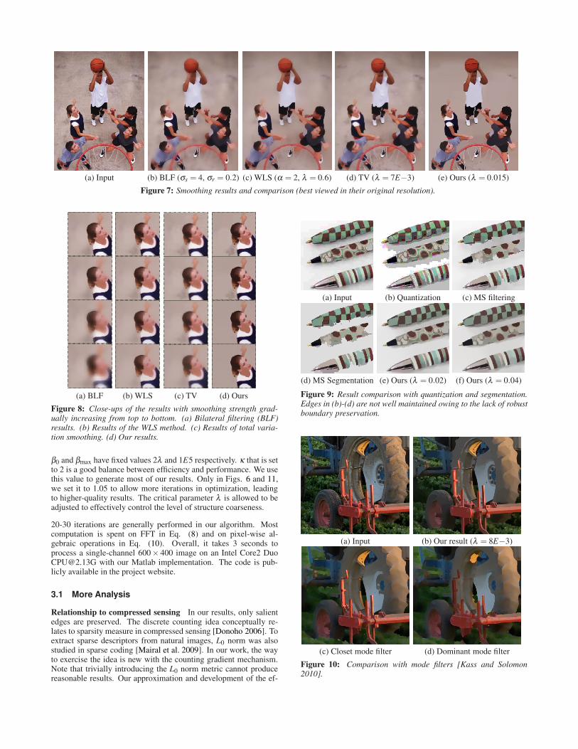
(a) Input (b) BLF (σs = 4, σr = 0.2) (c) WLS (α = 2, λ = 0.6) (d) TV (λ = 7E−3) (e) Ours (λ = 0.015)
Figure 7: Smoothing results and comparison (best viewed in their original resolution).
(a) BLF (b) WLS (c) TV (d) Ours
Figure 8: Close-ups of the results with smoothing strength grad-ually increasing from top to bottom. (a) Bilateral filtering (BLF)results. (b) Results of the WLS method. (c) Results of total varia-tion smoothing. (d) Our results.
β0 and βmax have fixed values 2λ and 1E5 respectively. κ that is setto 2 is a good balance between efficiency and performance. We usethis value to generate most of our results. Only in Figs. 6 and 11,we set it to 1.05 to allow more iterations in optimization, leadingto higher-quality results. The critical parameter λ is allowed to beadjusted to effectively control the level of structure coarseness.
20-30 iterations are generally performed in our algorithm. Mostcomputation is spent on FFT in Eq. (8) and on pixel-wise al-gebraic operations in Eq. (10). Overall, it takes 3 seconds toprocess a single-channel 600× 400 image on an Intel Core2 [email protected] with our Matlab implementation. The code is pub-licly available in the project website.
3.1 More Analysis
Relationship to compressed sensing In our results, only salientedges are preserved. The discrete counting idea conceptually re-lates to sparsity measure in compressed sensing [Donoho 2006]. Toextract sparse descriptors from natural images, L0 norm was alsostudied in sparse coding [Mairal et al. 2009]. In our work, the wayto exercise the idea is new with the counting gradient mechanism.Note that trivially introducing the L0 norm metric cannot producereasonable results. Our approximation and development of the ef-
(a) Input (b) Quantization (c) MS filtering
(d) MS Segmentation (e) Ours (λ = 0.02) (f) Ours (λ = 0.04)
Figure 9: Result comparison with quantization and segmentation.Edges in (b)-(d) are not well maintained owing to the lack of robustboundary preservation.
(a) Input (b) Our result (λ = 8E−3)
(c) Closet mode filter (d) Dominant mode filter
Figure 10: Comparison with mode filters [Kass and Solomon2010].

(a) Input (b) Ours (λ = 0.015, κ = 1.05)
(c) Gradient map of (a) (d) Gradient map of (b)
(e) Edge map of (a) (f) Edge map of (b)
Figure 11: Edge enhancement and extraction. Our method sup-presses low-amplitude details and enhances high contrast edges.The combined effect is to remove textures and sharpen main edgeseven if their gradient magnitudes are not significant locally.
fective algorithm to achieve sub-problem global optimization arecentral to the high practicality.
Difference with total variation and other regularizers Con-tinuous Lp norm with p = 1 was enforced in total variation (TV)smoothing to suppress noise. In this framework, strong smoothinginevitably curtails originally salient edges to penalize their magni-tudes. In our method, large gradient magnitudes are allowed bynature with our discrete counting measure.
Lp norm regularization with 0.5 ≤ p ≤ 1 was also employed in[Levin et al. 2007] to model the sparsity of natural image gradients.The success of the WLS optimization attributes in part to the Lpnorm in the Iterative Reweighed Least Square (IRLS) framework.Mathematically, Lp norm satisfies positive scalability constraint‖ax‖p
p = |a|p · ‖x‖pp , where a is a scalar. It yields ‖ax‖p
p > ‖x‖pp
if |a| > 1, which implies that these norms still impose large penal-ties on salient gradients. On the contrary, the L0 norm in Eq. (1)satisfies #{|x|> 0}= #{|ax|> 0} for any non-zero a, and thus doesnot comply with the positive scalability constraint. This major dif-ference leads to new smoothing behavior.
Selectively penalizing image gradients is also related to the WeakMembrane model of Blake and Zisserman [1987], which explicitlyrepresents discontinuity and adjusts gradients only in continuousregions. Our method is dissimilar in formulation and in solver.
A natural image example is shown in Fig. 7 with comparison withother state-of-the-art approaches. More are put in our project web-site, produced with different parameters. Close-ups in Fig. 8 areobtained by varying smoothing strength. Our results contain glob-ally the most salient structures in different degrees.
(a) Input (b) Gradients of (a) (c) Edges of (a)
(d) Ours (λ = 0.03) (e) Gradients of (d) (f) Edges of (d)
Figure 12: Smoothing for edge detection. The input image (a) con-tains complex structures, making edge extraction error-prone. Onour smoothed image (d), primary edges can be faithfully detectedusing the same edge detector.
Comparison to quantization and segmentation To clarify thedifference, we use the example shown in Fig. 9, where the natu-ral image contains a very small amount of noise, common in pho-tos. Color quantization can neither suppress noise nor accurately re-move details, yielding incorrect boundaries, as shown in Fig. 9(b).Image segmentation seeks proper spatial partitioning. This set ofmethods are widely known as difficult to maintain fine edges, inparticular for images with textures or details. Fig. 9(c) and (d) showthe results of mean-shift filtering [Comaniciu and Meer 2002] andof its segmentation – formed by fusing – after trying a variety ofparameters. The boundaries are not aligned with the latent edges.Our results produced with two λ values are shown in Fig. 9(e) and(f). Edges are better preserved.
Comparison to local histogram-mode filtering The method ofKass and Solomon [2010] is not based on smoothing neighboringpixels, and thus can sharpen edges while reducing details. We showin Fig. 10 a close-up comparison. The edges in our result (b) are inline with the originally salient ones due to the global optimization.
4 Applications
Our method avails several applications due to its fundamentalityand the special properties in processing natural images. We apply itto edge enhancement and extraction, non-photorealistic rendering,clip-art restoration, and layer decomposition based manipulation.
4.1 Edge Enhancement and Extraction
Edge extraction from natural images is a basic manipulationtool. Structured edges can be used for natural image editing[Bae and Durand 2007] and high-level structure inference. Highquality results that are continuous, accurate, and thin are generallyvery difficult to produce due to high susceptibility of edge detec-tors to complex structures and inevitable noise. Our method is ableto suppress low-amplitude details, which remarkably stabilizes theextraction process.
In the example shown in Fig. 11(a), the original ramp is visu-ally distinct due to its high contrast. But the boundaries are notvery sharp with overall small-magnitude gradients, making themindistinguishable from low-contrast details around. The gradientmagnitude image is shown in (c), linearly enhanced for visualiza-tion. Applying the Canny edge detector to the original image pro-duces a problematic result (e). Our method can remove statisti-

(a) (b)
Figure 13: Image abstraction and pencil sketching results. Ourmethod removes the least important structures.
cally insignificant details by global optimization. The remainingmain structures in (d) are in the meantime slightly sharpened withnotably amplified gradients. With these two main advantages, thedetected edges in our result using the same operator can be muchmore reliable, as shown in (f).
Fig. 12(a) shows another picture containing characters togetherwith background textures. Directly computing gradients on the in-put image acquires many unwanted small-amplitude structures, asshown in (b). They greatly affect binary Canny edge detector, asshown in (c). Character boundaries are broken; some are even in-correctly connected. Our smoothing result (d) has a cleaner gradi-ent map (e). The edges in (f) computed by the same detector aremuch better, in accordiance with human perception.
4.2 Image Abstraction and Pencil Sketching
Our smoothed image representation fits non-photorealistic abstrac-tion with simultaneous detail flattening and edge emphasizing. Twomain steps are involved in traditional methods – that is, imagesmoothing by mean-shift filtering [DeCarlo and Santella 2002] orbilateral filtering [Winnemoller et al. 2006], and line extraction bydifference-of-Gaussian (DoG) filtering. The extracted lines are en-hanced and are composed back to augment the visual distinctive-ness of different regions. Our method can simultaneously achievethe two goals. After smoothing images with a large λ weight, edgedetection can be directly applied.
In [2002], DeCarlo and Santella found that segmentation can-not faithfully preserve edges, and therefore employed a means tosmooth them. This is unnecessary for our approach since it glob-ally maintains edge position and magnitudes. Fig. 13 shows twoabstraction results.
We create pencil sketching also based on the extracted edge maps.Two results are shown in Fig. 13. They are produced by randomlyadding small sketchy lines to the extracted edges, along the tan-
Figure 14: Quantitative evaluation of clip-art JPEG artifact re-moval. X-axis: JPEG quality. Left Y-axis: PSNR. Right Y-axis:SSIM values.
gent direction. The sketchy lines are with constant length and withgray levels proportional to edge magnitudes. This simple approachenhances significant edges, making structures visually pleasing.
4.3 Clip-Art Compression Artifact Removal
Our smoothing method is also advantageous for cartoon/clip-artcompression artifact removal thanks to its special ability to enhanceedges. We have experimented with many cartoon/clip-art imageswith severe compression artifacts. To cope with them, prior knowl-edge and a training process are required in [Wang et al. 2006]. Oursmoothing method in contrast can reliably restore these degradedclip-arts without any learning procedure. The regularization weightλ in this case is set within [0.02,0.1]. Note that general denoisingapproaches do not suit this application as the compression artifactsare strongly correlated with edges.
We evaluate a set of methods, including edge-preserving smooth-ing, denoising [Rudin et al. 1992; Dabov et al. 2007], segmenta-tion, and image analogue-based method [Wang et al. 2006] for re-moving block-based discrete cosine transform (BDCT) artifacts onclip-art images, and show one comparison in Fig. 16.
(a) Input (b) [Wang et al. 2006] (c) MS (d) Our result
Figure 15: Cartoon restoration results of Wang et al. [2006],mean-shift (MS) segmentation, and of our method.
For quantitative comparison, we compressed 100 clip-art images bystandard JPEG with quality values ranging from 10 to 90, and cal-culated the peak signal-noise ratio (PSNR) and structural similar-ity (SSIM) [Wang et al. 2004] values after applying different meth-ods to restoration. The statistics are plotted in Fig. 14. Both thePSNR and SSIM scores indicate that our method performs well inremoving the JPEG artifacts. Note that the compression artifactslocally shift color, which inherently reduce PSNR. The SSIM plotsshow that some clip-art images compressed with quality 40, afterour restoration, can be structurally comparable to those with com-pression quality 90+. Fig. 15 shows another comparison.
4.4 Layer-Based Contrast Manipulation
Contrast expansion or compression enables detail magnifica-tion [Bae et al. 2006; Fattal et al. 2007] and HDR compression
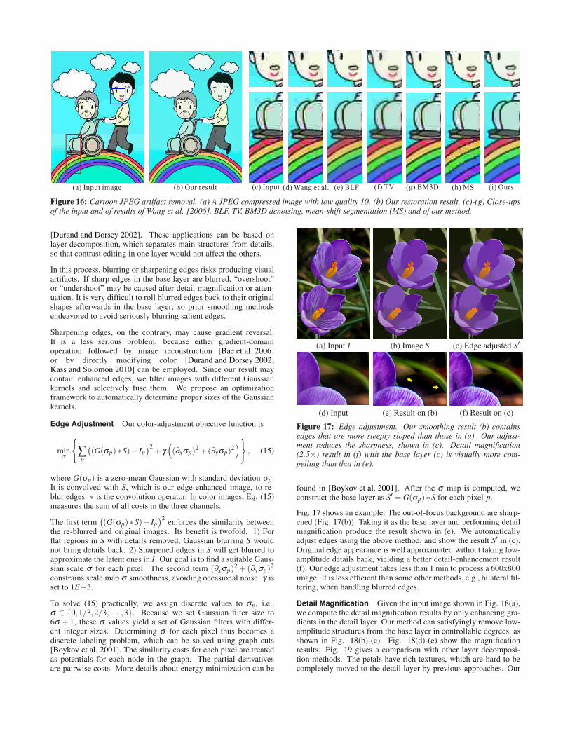
(a) Input image (b) Our result (c) Input (e) BLF(d) Wang et al. (h) MS (i) Ours(g) BM3D(f) TV
Figure 16: Cartoon JPEG artifact removal. (a) A JPEG compressed image with low quality 10. (b) Our restoration result. (c)-(g) Close-upsof the input and of results of Wang et al. [2006], BLF, TV, BM3D denoising, mean-shift segmentation (MS) and of our method.
[Durand and Dorsey 2002]. These applications can be based onlayer decomposition, which separates main structures from details,so that contrast editing in one layer would not affect the others.
In this process, blurring or sharpening edges risks producing visualartifacts. If sharp edges in the base layer are blurred, “overshoot”or “undershoot” may be caused after detail magnification or atten-uation. It is very difficult to roll blurred edges back to their originalshapes afterwards in the base layer; so prior smoothing methodsendeavored to avoid seriously blurring salient edges.
Sharpening edges, on the contrary, may cause gradient reversal.It is a less serious problem, because either gradient-domainoperation followed by image reconstruction [Bae et al. 2006]or by directly modifying color [Durand and Dorsey 2002;Kass and Solomon 2010] can be employed. Since our result maycontain enhanced edges, we filter images with different Gaussiankernels and selectively fuse them. We propose an optimizationframework to automatically determine proper sizes of the Gaussiankernels.
Edge Adjustment Our color-adjustment objective function is
minσ
{∑p
((G(σp)∗S)− Ip
)2 + γ((∂xσp)2 +(∂yσp)2
)}, (15)
where G(σp) is a zero-mean Gaussian with standard deviation σp.It is convolved with S, which is our edge-enhanced image, to re-blur edges. ∗ is the convolution operator. In color images, Eq. (15)measures the sum of all costs in the three channels.
The first term((G(σp)∗S)− Ip
)2 enforces the similarity betweenthe re-blurred and original images. Its benefit is twofold. 1) Forflat regions in S with details removed, Gaussian blurring S wouldnot bring details back. 2) Sharpened edges in S will get blurred toapproximate the latent ones in I. Our goal is to find a suitable Gaus-sian scale σ for each pixel. The second term (∂xσp)2 + (∂yσp)2
constrains scale map σ smoothness, avoiding occasional noise. γ isset to 1E−3.
To solve (15) practically, we assign discrete values to σp, i.e.,σ ∈ {0,1/3,2/3, · · · ,3}. Because we set Gaussian filter size to6σ + 1, these σ values yield a set of Gaussian filters with differ-ent integer sizes. Determining σ for each pixel thus becomes adiscrete labeling problem, which can be solved using graph cuts[Boykov et al. 2001]. The similarity costs for each pixel are treatedas potentials for each node in the graph. The partial derivativesare pairwise costs. More details about energy minimization can be
(a) Input I (b) Image S (c) Edge adjusted S′
(d) Input (e) Result on (b) (f) Result on (c)
Figure 17: Edge adjustment. Our smoothing result (b) containsedges that are more steeply sloped than those in (a). Our adjust-ment reduces the sharpness, shown in (c). Detail magnification(2.5×) result in (f) with the base layer (c) is visually more com-pelling than that in (e).
found in [Boykov et al. 2001]. After the σ map is computed, weconstruct the base layer as S′ = G(σp)∗S for each pixel p.
Fig. 17 shows an example. The out-of-focus background are sharp-ened (Fig. 17(b)). Taking it as the base layer and performing detailmagnification produce the result shown in (e). We automaticallyadjust edges using the above method, and show the result S′ in (c).Original edge appearance is well approximated without taking low-amplitude details back, yielding a better detail-enhancement result(f). Our edge adjustment takes less than 1 min to process a 600x800image. It is less efficient than some other methods, e.g., bilateral fil-tering, when handling blurred edges.
Detail Magnification Given the input image shown in Fig. 18(a),we compute the detail magnification results by only enhancing gra-dients in the detail layer. Our method can satisfyingly remove low-amplitude structures from the base layer in controllable degrees, asshown in Fig. 18(b)-(c). Fig. 18(d)-(e) show the magnificationresults. Fig. 19 gives a comparison with other layer decomposi-tion methods. The petals have rich textures, which are hard to becompletely moved to the detail layer by previous approaches. Our

(a) Input (b) Base layer (λ = 7E−3) (c) Base layer (λ = 2E−2) (d) Boosted from (b) (e) Boosted from (c)
Figure 18: Base-detail separation and manipulation. (a) Input image. (b)-(c) Two base layers generated by our method. (d)-(e) Detailmagnification results with (b) and (c) being the base layers respectively.
(a) LCIS (b) BLF (c) WLS (d) TV (e) Ours
Figure 19: Base-detail separation and manipulation. From top to bottom: the base layers, the detail enhanced results (2.5×), and close-ups. Parameters: LCIS (n = 1000, k = 0.25 for diffuse Kval, t = 1 for diffuse Tstep), BLF (σs = 4, σr=0.2), WLS (α = 1.2, λ = 0.8), TV(λ = 2E−2), and ours (λ = 3E−2).
(a) BLF [Durand and Dorsey 2002] (b) WLS [Farbman et al. 2008] (c) [Subr et al. 2009] (d) Ours
Figure 20: Tone mapping results.

(a) Tone mapping (λ = 0.4) (b) Tone mapping (λ = 0.07)
Figure 21: An excessively large λ causes unnatural reflection in (a)in tone mapping. Result (b) is produced with a more appropriate λ .
(a) Input (b) Ours
(c) BLF (d) BLF + Ours
Figure 22: Novel smoothing effect to remove small-resolutionstructures that are with large amplitudes. We propose applying bi-lateral filtering and our method consecutively to accomplish it.
result contains nearly no low-amplitude edges, and no blurriness iscaused. More results are in the project website.
Tone Mapping HDR tone mapping is another popular ap-plication that can be achieved by decomposing an HDRimage into a piece-wise smooth base layer conveying mostof the energy and a detail layer [Tumblin and Turk 1999;Durand and Dorsey 2002; Choudhury and Tumblin 2003;Li et al. 2005; Farbman et al. 2008]. The base layer is thennonlinearly mapped to a low dynamic range and is re-combinedwith the detail layer. The base layer is required to preserve sharpdiscontinuities to avoid halos [Tumblin and Turk 1999] and besmooth enough for reasonable contrast maintenance in rangecompression, as discussed in [Choudhury and Tumblin 2003].
In the tone mapping framework of Durand and Dorsey [2002], weuse our smoothing method for layer decomposition, which is ap-plied to the logarithmic HDR images. One result is shown in Fig.20. Structures are preserved or enhanced in the tone mapped image.
It is notable that the quality of tone mapping results can be affectedby parameter tuning in our layer decomposition. It is possible for
(a) Input (b) Smoothing result
(c) Edge adjusted (d) Detail magnification
Figure 23: Wide illumination transition. Using a large λ in ourmethod makes textures be removed; the result is shown in (b). Basedon it, layer-based detail enhancement is achieved, shown in (d).
some results to present visual artifacts when the smoothing weightλ is not appropriately set. One example is shown in Fig. 21(a),where the floor is with a blocky reflection. It is caused by apply-ing strong smoothing, which sends structures excessively to the de-tail layer, making smooth gradients be flattened. Using a smallerweight can dampen the problem, as illustrated in the result (b).
5 Discussion and Limitations
We have presented a well-principled and powerful smoothingmethod based on the mechanism of discretely counting spatialchanges, which can remove low-amplitude structures and globallypreserve and enhance salient edges, even if they are boundaries ofvery narrow objects.
As our system does not use spatial filtering or averaging, it canbe regarded as complementary to previous local approaches. In-terestingly, when combined with local filtering, our method canproduce novel effects. For the example shown in Fig. 22, apply-ing our method alone remains part of the fluff texture because it iswith high amplitude. Only bilaterally filtering the image contrarilyblurs main boundaries under strong smoothing. We propose firstapplying bilateral filtering, which lowers the amplitudes of noise-like structures more than those of long coherent edges, followed byour method to globally sharpen prominent edges. Result in (d) onlycontains large-scale salient edges, profiting main structure extrac-tion and understanding.
Limitations Over-sharpening is sometimes unavoidable in chal-lenging circumstances to remove details. In the example shown inFig. 23, strong illumination variation spans many pixels. To re-move textures, our method may produce an over-sharpened result,as exemplified in (b). This result, however, can still be used in detailmagnification. After edge adjustment as described in Sec. 4.4 andtaking the result as the base layer, we magnify only details. Thefinal result is shown in Fig.23(d). The aforementioned parametertuning for tone mapping is another limitation.

Acknowledgements
We thank Michael S. Brown for his help in making the video, andthe following people and flicker users for the photos used in thepaper: John McCormick, conner395, cyber-seb, T-KONI, RemiLongva, dms a jem. This work is supported by a grant from theResearch Grants Council of the Hong Kong SAR (project No.413110).
References
ARBELAEZ, P., MAIRE, M., FOWLKES, C., AND MALIK, J.2011. Contour detection and hierarchical image segmentation.IEEE Trans. Pattern Anal. Mach. Intell. 33, 898–916.
BAE, S., AND DURAND, F. 2007. Defocus magnification. Comput.Graph. Forum 26, 3, 571–579.
BAE, S., PARIS, S., AND DURAND, F. 2006. Two-scale tonemanagement for photographic look. ACM Trans. Graph. 25, 3,637–645.
BAEK, J., AND JACOBS, D. E. 2010. Accelerating spatially vary-ing gaussian filters. ACM Trans. Graph..
BLACK, M. J., SAPIRO, G., MARIMONT, D. H., AND HEEGER,D. 1998. Robust anisotropic diffusion. IEEE Transactions onImage Processing 7, 3, 421–432.
BLAKE, A., AND ZISSERMAN, A. 1987. Visual reconstruction.The MIT Press.
BOYKOV, Y., VEKSLER, O., AND ZABIH, R. 2001. Fast approx-imate energy minimization via graph cuts. IEEE Trans. PatternAnal. Mach. Intell. 23, 11, 1222–1239.
CHEN, J., PARIS, S., AND DURAND, F. 2007. Real-time edge-aware image processing with the bilateral grid. ACM Trans.Graph. 26, 3, 103.
CHOUDHURY, P., AND TUMBLIN, J. 2003. The trilateral filterfor high contrast images and meshes. In Rendering Techniques,186–196.
COMANICIU, D., AND MEER, P. 2002. Mean shift: A robustapproach toward feature space analysis. IEEE Trans. PatternAnal. Mach. Intell. 24, 5, 603–619.
CRIMINISI, A., SHARP, T., ROTHER, C., AND PEREZ, P. 2010.Geodesic image and video editing. ACM Trans. Graph. 29, 5,134.
DABOV, K., FOI, A., KATKOVNIK, V., AND EGIAZARIAN, K. O.2007. Image denoising by sparse 3-d transform-domain collab-orative filtering. IEEE Transactions on Image Processing 16, 8,2080–2095.
DECARLO, D., AND SANTELLA, A. 2002. Stylization and ab-straction of photographs. ACM Trans. Graph. 21, 3, 769–776.
DONOHO, D. 2006. Compressed sensing. IEEE Transactions onInformation Theory 52, 4, 1289–1306.
DURAND, F., AND DORSEY, J. 2002. Fast bilateral filtering forthe display of high-dynamic-range images. ACM Trans. Graph.21, 3, 257–266.
FARBMAN, Z., FATTAL, R., LISCHINSKI, D., AND SZELISKI, R.2008. Edge-preserving decompositions for multi-scale tone anddetail manipulation. ACM Trans. Graph. 27, 3.
FARBMAN, Z., FATTAL, R., AND LISCHINSKI, D. 2010. Diffu-sion maps for edge-aware image editing. ACM Trans. Graph..
FATTAL, R., AGRAWALA, M., AND RUSINKIEWICZ, S. 2007.Multiscale shape and detail enhancement from multi-light imagecollections. ACM Trans. Graph. 26, 3, 51.
FATTAL, R. 2009. Edge-avoiding wavelets and their applications.
ACM Trans. Graph. 28, 3.KASS, M., AND SOLOMON, J. 2010. Smoothed local histogram
filters. ACM Trans. Graph. 29, 4.LEVIN, A., LISCHINSKI, D., AND WEISS, Y. 2004. Colorization
using optimization. ACM Trans. Graph. 23, 3, 689–694.LEVIN, A., FERGUS, R., DURAND, F., AND FREEMAN, W. T.
2007. Image and depth from a conventional camera with a codedaperture. ACM Trans. Graph. 26, 3, 70.
LI, Y., SUN, J., TANG, C.-K., AND SHUM, H.-Y. 2004. Lazysnapping. ACM Trans. Graph. 23, 3, 303–308.
LI, Y., SHARAN, L., AND ADELSON, E. H. 2005. Compress-ing and companding high dynamic range images with subbandarchitectures. ACM Trans. Graph. 24, 3, 836–844.
LISCHINSKI, D., FARBMAN, Z., UYTTENDAELE, M., ANDSZELISKI, R. 2006. Interactive local adjustment of tonal val-ues. ACM Trans. Graph. 25, 3, 646–653.
LIU, J., SUN, J., AND SHUM, H.-Y. 2009. Paint selection. ACMTrans. Graph. 28, 3.
MAIRAL, J., BACH, F., PONCE, J., SAPIRO, G., AND ZISSER-MAN, A. 2009. Non-local sparse models for image restoration.In ICCV, 2272–2279.
MAJI, S., VISHNOI, N., AND MALIK, J. 2011. Biased normalizedcuts. In CVPR.
PARIS, S., AND DURAND, F. 2006. A fast approximation of thebilateral filter using a signal processing approach. In ECCV (4),568–580.
PARIS, S., HASINOFF, S. W., AND KAUTZ, J. 2011. Local lapla-cian filters: Edge-aware image processing with a laplacian pyra-mid. ACM Trans. Graph..
PERONA, P., AND MALIK, J. 1990. Scale-space and edge detectionusing anisotropic diffusion. IEEE Trans. Pattern Anal. Mach.Intell. 12, 7, 629–639.
ROTHER, C., KOLMOGOROV, V., AND BLAKE, A. 2004. ”grab-cut”: interactive foreground extraction using iterated graph cuts.ACM Trans. Graph. 23, 3, 309–314.
RUDIN, L., OSHER, S., AND FATEMI, E. 1992. Nonlinear totalvariation based noise removal algorithms. Physica D: NonlinearPhenomena 60, 1-4, 259–268.
SUBR, K., SOLER, C., AND DURAND, F. 2009. Edge-preservingmultiscale image decomposition based on local extrema. ACMTrans. Graph. 28, 5.
TOMASI, C., AND MANDUCHI, R. 1998. Bilateral filtering forgray and color images. In ICCV, 839–846.
TUMBLIN, J., AND TURK, G. 1999. Lcis: A boundary hierarchyfor detail-preserving contrast reduction. In SIGGRAPH, 83–90.
WANG, Z., BOVIK, A. C., SHEIKH, H. R., AND SIMONCELLI,E. P. 2004. Image quality assessment: from error visibility tostructural similarity. IEEE Transactions on Image Processing13, 4, 600–612.
WANG, G., WONG, T.-T., AND HENG, P.-A. 2006. Deringingcartoons by image analogies. ACM Trans. Graph. 25, 4, 1360–1379.
WANG, Y., YANG, J., YIN, W., AND ZHANG, Y. 2008. A newalternating minimization algorithm for total variation image re-construction. SIAM J. Imaging Sciences 1, 3, 248–272.
WEISS, B. 2006. Fast median and bilateral filtering. ACM Trans.Graph. 25, 3, 519–526.
WINNEMOLLER, H., OLSEN, S. C., AND GOOCH, B. 2006. Real-time video abstraction. ACM Trans. Graph. 25, 3, 1221–1226.